Model for clustering of living species

Abstract

Clusters appear in nature in a diversity of contexts, involving distances as long as the cosmological ones, and down to atoms and molecules and the very small nuclear size. They also appear in several other scenarios, in particular in biological systems as in ants, bees, birds, fishes, gnus and rats, for instance. Here we describe a model composed of a set of female and male individuals that obeys simple rules that rapidly transform an uniform initial state into a single cluster that evolves in time as a stable dynamical structure. We show that the center of mass of the structure moves as a random walk, and that the size of the cluster engenders a power law behavior in terms of the number of individuals in the system. Moreover, we also examine other possibilities, in particular the case of two distinct species that can evolve to form one or two distinct clusters.

1 Introduction

Clusters appear in nature in several distinct situations. At very large scales, the Universe, for instance, is known to be arranged in the form of clusters of galaxies, and the galaxies themselves are clusters of gas, dust, stars and their planetary systems; see, e.g., Ref. [1]. At very small scales, at the nuclear level, for instance, the nuclear matter aggregates to form the atomic nuclei, which may also contain clusters of deuterons, tritons and alpha particles; see, e.g., Ref. [2]. As one knows, at the atomic and molecular level, nuclei and electrons also aggregate to form atoms and molecules. And more, clusters also appear in several other scenarios: in economics, they may engender a strategy to improve productivity [3]; in social networks, they may help control specific features such as disease spreading [4]; and they may also play a role in data control and mining [5, 6] and in several other areas of research of current interest.

We may say that clusters are also of interest in living systems such as ants, bees, birds and fishes, among others; see, e.g., Refs. [7, 8, 9, 10] and references therein. In ants and bees, the individuals tend to cluster in the presence of at least one distinct individual, but this is not the case for birds and fishes, for instance, since each species seems to have no particular individual to lead or conduct the group. In this sense, the study of clusters and the investigation of clustering mechanisms is of great interest in science in general and, in particular, in the case of living systems. As one knows, living in groups may engender the advantage of a lower predation risk and better efficiency when seeking for food, but may also enhance competition for food itself, and increase the risk of illness due to the spread of diseases, among other things; see, e.g., Refs. [11, 12, 13, 14, 15, 16] and references therein for recent studies on the subject.

In this work we concentrate on the presence of clusters in a simple system composed of a set of female and male individuals of a single species that can move, and die or reproduce at a given rate. We introduce no preference or distinction among the many individuals, so the system is somehow closer to birds, cockroaches, fishes, gnus or rats, for instance. We shall deal with a two-dimensional distribution of individuals in a square box, so the model will be closer to cockroaches, gnus or rats, among other possibilities. We also notice the occurrence of sexual processes in bacteria such as the Escherichia Coli [17, 18], so the model may be of interest at the bacterial level as well.

In order to examine issues related to the presence of clusters in living systems, we start the work with a two-dimensional system of individuals, searching for a mechanism that leads to the clustering of the individuals into a state that is dynamically stable. We describe the system in the Sec. Model and study its time evolution in Sec. Results, where one shows the results for the cluster formation, and some of its features. We examine other interesting possibilities in Sec. Other Results and end the work with some conclusions and open questions.

2 Model

The model to be investigated is initially composed of a set of $N$ individuals, with $N/2$ being female and $N/2$ male. In this work we only deal with species in which the individuals are either female or male for their entire lifetime, with the initial state being prepared with the total number of individuals distributed randomly in a square box of linear size $L=1$. The spatial distribution of individuals is described as an off-lattice model, in a way similar to the off-lattice model considered before in [19, 20]. In other words, the space is continuum here, in distinction to the discrete lattice model which will not be considered in this work. Due to the random distribution, the initial state represents an uniform distribution of individuals. The system obeys periodic boundary conditions, and the time evolution starts with a time step in which one randomly selects an individual, which is the active individual. It is then moved with a fixed step defined by the distance $\ell=0.01$, in a direction that is chosen randomly. After the motion, an action is selected with the following probabilities: $p_{r}$ or $p_{d}$, for the individual to reproduce or die, respectively. They are associated to reproduction or extermination, and the real world is of course much more complex than this, but here $p_{d}$ is used to describe predation on general grounds, and $p_{r}$ on the contrary is to keep the system alive.

When $p_{d}$ is chosen, the active individual is removed from the system. However, when $p_{r}$ is chosen, one verifies if there is an individual of the opposite sex is the region inside the circle of radius $\ell$ around the active individual; if there is no individual we restart choosing another active individual, but if there are more than one individual of the opposite sex in the region one chooses the closest one. The next step is to check the total number of individuals: if it is less than $N$, a new individual is born, which is chosen to be female or male with equal probability. This individual is put inside the box, at the distance $\ell$ of the female, in a direction which is also chosen randomly. We have to choose $p_{d}<p_{r}$, and here we take $p_{d}=0.3$ and $p_{r}=0.7$. This choice favours reproduction, so to avoid an indefinite increasing in the number of individuals, we add the constraint that the total number of individuals should not overcome $N$.

We notice that the proximity parameter $\ell$ is introduced to unveil the scale of reproduction. It is responsible for the grouping of female and male into the cluster and describes a very simple mathematical model, capable of conducting complex collective phenomena based on very simple mathematical rules. Since no other specific biological characteristics is attributed to the individuals in the model, we cannot use it to describe any specific group of living species. However, it will trigger a mechanism that leads to a complex clustering phenomenon, which will be further explored in this work. The motivation here is similar to the ones included in Refs. [12, 13, 21, 22, 23, 24], for instance, which also deal with simple mathematical models that may be able to describe complex behaviors in evolutionary game theory. We recall, in particular, the review on the study of evolutionary dynamics of group interactions on structured populations, complex networks and coevolutionary models [12], results showing that smart and tolerant species have more efficient networks [13], the investigation where specific types of reciprocity norms may lead individuals to split into groups in which they are cooperative [22], the study of topological frustration on the evolutionary dynamics of the snowdrift game on a triangular lattice [23], and also the recent review on human cooperation, with focus on spatial pattern formation, on the time evolution of observed solutions, and on other behaviors that may either promote or hinder socially favorable states [24].

In this work, we run the numerical simulations using $t$ to provide the time evolution in terms of generations, with one generation being the time spent during the occurrence of $N$ time steps. We notice that the square box of linear size $L$ describes a two-dimensional off-lattice model, and we understand the distance $\ell$ as the parameter that sets the scale of proximity between partners in the system. In particular, we notice that $p_{d}$ occurs by chance, so it cannot be seen as a behavioural characteristic of the individuals. However, $p_{r}$ only occurs in the presence of the closest partner, inside the circular region of radius $\ell$, if the total number of individuals is below $N$, so the proximity parameter $\ell$ defines the behavioural zone and acts to make $p_{r}$ a behavioural parameter. As we shall show in Sec. Results, the above rules together favour the extermination of isolated individuals and the grouping of partners into a cluster that collects all the individuals of the system.

3 Results

We have implemented many numerical simulations, and in Fig. 1 four distinct snapshots are depicted to illustrate the time evolution of the system with $N=1000$ individuals. The first snapshot at the top left represents a typical initial state of the system. In this figure, it is possible to verify that after some generations the system starts to form small clusters, which evolve into larger ones, in an evolution that ends up with a single larger cluster containing all the $N$ individuals present in the initial state. We can understand this with the fact that in a larger cluster, the probability to implement the rule reproduction increases due to the increasing of individuals in the cluster, when compared to smaller clusters. The rules used to describe the time evolution of the system seems to describe a very efficient algorithm to cluster or aggregate the individuals into a small region inside the box, so we move on to study the basic properties of the system.

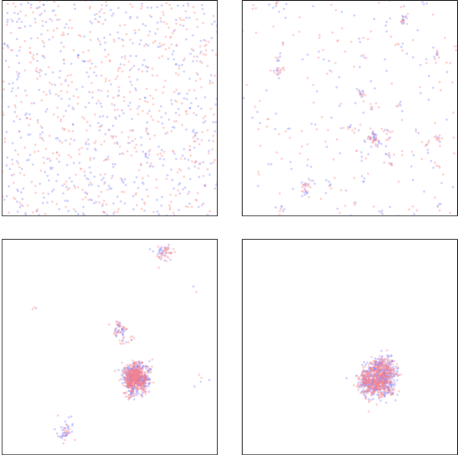
Figure 1: Snapshots of the spatial distribution of females (red) and males (blue) at the generation times $t=0$ (top left), $t=5$ (top right), $t=25$ (bottom left), and $t=125$ (bottom right). One notices the formation of clusters, with only one cluster surviving when time goes beyond one hundred generations.

In Fig. 2 we examine the time evolution of the abundance or density of female ($\rho_{f}(t)$) and male $(\rho_{m}(t))$ individuals. We run a simulation using $N=1000$ up to $t=1000$ generations and depict the results with the red and blue colors that represent the female and male, respectively. The results show that they evolve fluctuating around their average values $\langle{\rho}_{f}\rangle=\langle{\rho}_{m}\rangle=0.5$ for very long times, indicating the dynamical robustness of the time evolution of the system. In fact, we tested the abundance for much longer times, for $t=10000$, $20000$, $30000$, $40000$ and $50000$ generations, and we found no important deviation from the behavior displayed in Fig. 2. This suggests that the system rapidly evolves to reach dynamical stability. However, we noticed that the simulation started with a very large and abrupt variation of abundance, but we can understand this as follows: initially, the individuals are on average well separated from each other, favouring that the ratio of dead overcomes reproduction, but this is soon modified due to the clustering mechanism and the system rapidly returns to its dynamical stability, with the abundances oscillating around their average with small fluctuations. Female and male evolve on equal footing, so they have similar behavior and the very same average abundance.

The results displayed in Figs. 1 and 2 show that the system rapidly evolves grouping all the individuals into a single cluster, which seems to evolve robustly for very long times. For this reason, let us now concentrate on the behavior of the cluster that is formed as the final state of the system. The first step concerned the calculation of the center of mass of the system, supposing that all the individuals carry the same mass. The calculation follows the method suggested in [25], which takes into account the periodic boundary conditions that we are using in this work. Since the system evolves in time, the center of mass coordinates are $(x_{CM}(t),y_{CM}(t))$, and follows the trajectory displayed in Fig. 3, colored in accordance with the time evolution that appears at the right of the figure. After a hundred generations the cluster is generated, and then its center of mass position evolves behaving like a random walk, illustrated by the colors yellow, red, blue and green in the figure. We notice, however, that the center of mass moves rapidly at the beginning of the simulation, before the formation of the cluster.

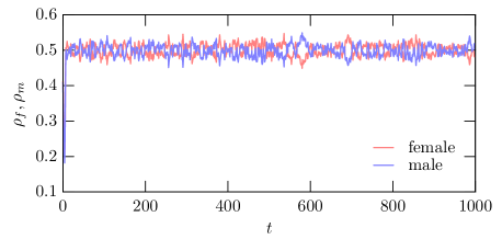
Figure 2: The female (red) and male (blue) abundances are displayed as a function of time for a long time.

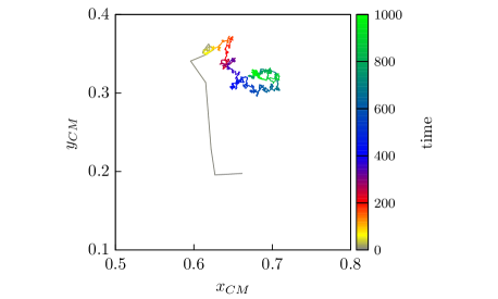
Figure 3: The position of the center of mass is shown as a functions of time.

We remark that the two Figs. 2 and 3 were constructed using results of a single realization, in fact the very same realization used to depict Fig. 1. Moreover, to certify that the center of mass position shown in Fig. 3 moves like a random walk for larger values of the time evolution, we have depicted in Fig. 4 the center of mass mean squared displacement (MSD), which was calculated as follows: we first discard the $1000$ first positions of the center of mass, to ensure that the cluster is already formed, then we start counting the time and at $t$ we calculate the MSD from the $1000$ center of mass positions, since we are simulating the system $1000$ times. We do this for several values of $t$ in order to calculate the mean square displacement. We call it $\langle[r(t)-r(0)]^{2}\rangle$ and depict the results with the light blue dots in the figure. The results shows that the MSD varies linearly on time which is characteristic of Brownian motion [26]. The error is due to the fitting procedure. The bins in Fig. 4 represent the error bars that account for the procedure to calculate the numerical values. We notice that the linear behavior displayed in Fig. 4 persists for a very long time, up to $100000$ generations, once again indicating the dynamical stability of the cluster.

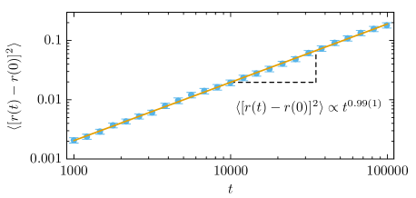
Figure 4: The center of mass mean square displacement of the cluster as a function of time for a very long time.

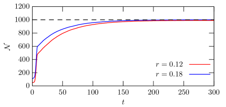
Figure 5: Number of individuals inside a circle of radius $r$ and center at the center of mass position of the system, depicted for $r=0.12$ and $0.18$.

The appearance of very large fluctuations at early times, as shown in Fig. 2, and the identification in Fig. 3 that the center of mass moves very rapidly at the beginning of the simulations has driven our attention to double check the numerical simulations. In particular, we display in Fig. 5 the number ${\mathcal{N}}$ of individuals inside a circle of radius $r$ and center at the center of mass position of the system as a function of time. The figure is depicted for $N=1000$ individuals, with $r=0.12$ (red) and $0.18$ (blue), with the data coming from an average over $1000$ simulations. The values of $r$ are chosen to lead to circles that fill $5$ and $10$ percent of the total area of the square box of linear size $L=1$, respectively. As expected, the initial evolution is abrupt, but the system rapidly evolves to approach a smooth time evolution which ultimately leads to the cluster formation. We also notice from Fig. 5 that the red and blue curves behave very similarly, and that almost all of the individuals are inside the smaller circle when $t$ approaches 200 generations.

We further noticed that if the density of individuals at the initial state is sufficiently small, the average distance among individuals may be sufficiently large to make the ratio of dead overcome reproduction with no return, that is, conducting the system to extinction. To examine this issue appropriately, we have studied the extinction probability $P_{\textrm{ext}}$ as a function of the number of individuals $N$ for many distinct values of $N$, always starting with an initial state which is constructed randomly, as described in Sec. Model. The results are depicted in Fig. 6 for three distinct values of $\ell$, to show how the proximity parameter changes the behavior of the system. We notice that the extinction probability vanishes and the system evolves in time keeping coexistence between female and male for appropriate values of $\ell$ and $N$. However, as we suspected, the probability of extinction increases as one decreases the number of individuals. Each dot displayed in Fig. 6 is calculated as the average in a set of $10000$ simulations, with all the simulations evolved for $1000$ generations. At the end of each simulation, we verified for the vanishing of individuals, or the presence of individuals of a single sex since this also implies extinction. The results displayed in Fig. 6 show that for the box with unity linear size $L=1$, the use of the distance $\ell=0.01$ is of interest if one takes $N=1000$ or other higher values. This will be used below to describe other features of the system.

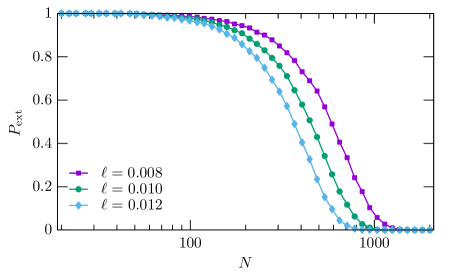
Figure 6: Extinction probability as a function of the number of individuals, depicted for $\ell=0.008$, $0.01$ and $0.012$.

In order to further examine the cluster, we have studied the distribution of distance of the individuals to the center of mass. The Fig. 7 shows this distribution for all the individuals. These results are obtained for several values of $N$, and they are calculated as an average of $1000$ distinct simulations for each value of $N$, for $1000$ generations.

With the results shown in Fig. 7, we could quantify the size of the cluster in terms of the number of individuals, which is depicted in Fig. 8. It is calculated as the width at half of its maximum height, and the results nicely show a power law behavior, that is, the size of the cluster is proportional to the number of individuals to the power $\alpha$, in the form $\bar{r}\propto N^{\alpha}$, with $\alpha=0.31(1)$, with the error in $\alpha$ being dictated by the fit. The error bars in Fig. 8 are due to the numerical simulations and are represented by the size of the bins in the figure.

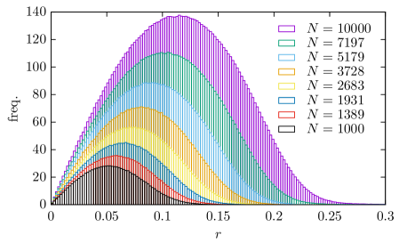
Figure 7: Histogram of the distribution of distance of the individuals to the center of mass of the cluster for several values of $N$.

4 Other results

Let us now examine the above model under other conditions. We first considered other values of $p_{r}$ and $p_{d}$; in particular, we used $p_{r}=0.8$ and $p_{d}=0.2$ and $p_{r}=0.9$ and $p_{d}=0.1$ and noticed no important qualitative difference from the results described above. We also observed that in the histograms displayed in Fig. 7, the distribution of frequency follows an interesting pattern, and this instigated us to study the issue more accurately. We first noticed that the highest frequency depends on the number of individuals, so we studied this to depict in Fig. 9 the function $f_{\rm max}(N)$, which represents the highest frequency in terms of the number of individuals. Interestingly, the results show that it depends on $N$ in the form of a power law, with power $0.69(1)$.

The above model considers female and male on an equal footing. However, since sex ratio varies widely in nature we can choose other possibilities; see, e.g., Ref. [27] and references therein. We first considered the same rules, but started with the initial state with female and male unevenly distributed. We used several possibilities, such as $0.6$ and $0.4$, $0.7$ and $0.3$, and $0.8$ and $0.2$, for female and male, for instance. In all cases the system always relax to a single cluster with equal distribution of female and male individuals. We also investigated the case where reproduction evolves under the male-biased rate of $0.55$; that is, when an individual is selected to be born, there is higher $55\%$ chance that a male will be born. We examined the numerical simulation in this case, and found that the system also develop a single cluster, but now keeping the very same bias: the abundance fluctuates around $55\%$ male and $45\%$ female. Alternatively, we kept the same rule of the previous Sec. Model for reproduction, but we changed $p_{d}$ as follows: when $p_{d}$ is selected, it is effectively implemented with the rate $50\%$ if the individual is a male, and with the full rate $100\%$ in the case of a female. The results showed that the system evolves to form a cluster, but now with the abundance of female and male fluctuating around $1/3$ and $2/3$, respectively. These results show that if there is no sex-biased rule, the system evolves to form a cluster with female and male evenly distributed; however, when a sex-biased rule is present, the system also form a cluster, but now with female and male distributed under the same bias.

We have also enlarged the system to consider two distinct species, one of them being the $1000$ red and blue individuals, and the other $1000$ yellow and green individuals. We suppose that they live together in a square box of unity linear size, and obey the very same rules described in Sec. Model, but now we add another constraint in the reproduction: any individual can only reproduce if inside the area with $\ell=0.01$, there is no individual of the other species. This adds a repulsion between the two species, which contributes to the formation of two distinct and spatially separated clusters, that evolve independently, with the very same characteristics that we have already identified in Sec. Results. Some results are displayed in Fig. 10, where we show the initial state at $t=0$, and its evolution at $t=5$, $25$, and $125$. We compare this with Fig. 1 to see that the system now relaxes to two distinct spatial clusters that evolve as two stable structures, independent from one another. The two distinct clusters are formed when we keep the initial number of individuals in each species as its upper bound for reproduction; however, if we choose the initial total number of individuals in the two species as the upper bound for reproduction, the system always relax to a single cluster with all the individuals of the same species, exterminating the other species. The two situations are quite distinct: the first case may be more appropriate to describe two distinct species that have independent constraints for reproduction; the second case is different, and is more appropriate to describe two distinct species that have the same constraint for reproduction.

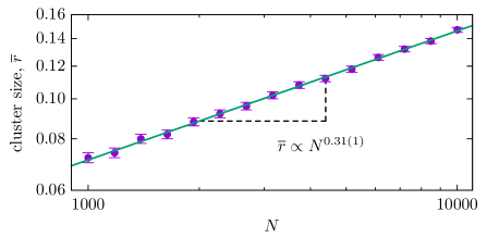
Figure 8: Cluster size as a functions of the number of individuals.

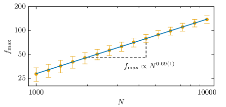
Figure 9: The highest frequency as a functions of the number of individuals.

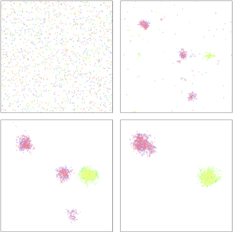
Figure 10: Snapshots of the spatial distribution of females (red/yellow) and males (blue/green) at the generation times $t=0$ (top left), $t=5$ (top right), $t=25$ (bottom left), and $t=125$ (bottom right). One notices the formation of clusters, with only two clusters surviving when time goes beyond one hundred generations.

5 Conclusion

In this work we investigated a simple model that describes a set of $N$ female and male individuals that are arranged in a off-lattice square box of linear size $L$. The individuals may die or reproduce, with the reproduction only occurring if the partner individual is very close to the active individual. We have used appropriate values to describe the number of individuals, the size of the box and the partner proximity, and to quantify the probabilities to die or reproduce. We run the numerical simulations for very long times, and the results suggested that the system rapidly evolves into a cluster that is dynamically stable. In particular, we calculated the abundances of female and male, and found that they evolve similarly, fluctuating around the same average as time goes by.

We also calculated the center of mass position of the cluster, which showed a behavior that approaches a random walk motion when one runs the simulations for a long time. Since both the abundance and the center of mass motion have peculiar behavior in the beginning of the simulations, we also investigated the extinction probability of the individuals as a function of the number of individuals, keeping the box size $L$ fixed and using three distinct values of the proximity parameter $\ell$. The general result here is that for a given $\ell$, small values of $N$ may drive the system to extinction, but we have a lot of room to choose $N$ to keep the system evolving from the uniform initial state to a cluster which is dynamically stable. The size of the cluster was also investigated for $L$ and $\ell$ fixed. We calculated the distribution of distance of the individuals to the center of mass, from which we obtained the mean square displacement of the cluster. The results unveiled a dependence on $N$ that follows a power law behavior.

We have also considered some modifications in the initial state and on the rules. In particular, if we keep the same rules and consider an initial state with female and male unevenly distributed, we end up with a stable cluster composed of female and male evenly distributed inside the structure. Also, if we consider sex-biased rules, the cluster is also formed and is also dynamically stable, but it now keeps female and male with the same bias provided by the sex-biased modification. We have also considered two distinct species, adding a very simple modification in the rule of reproduction. The modification may make the system to evolve with the formation of two distinct clusters, one for each species, or, else, a single cluster composed of only one of the two species. The two cases are of current interest, and the case with the formation of two independent clusters allows that we examine coexistence of two distinct species, which can also be extended to several species.

Since the clustering mechanism used in this work is simple, we may add other more sophisticated rules to help us understand specific features of clusters of living systems. We can, in particular, consider the case of groups of simple organisms that reproduces using the doubling mechanism, and also of groups of several distinct individuals that interact with one another, among other possibilities. We can also change the behavioural rule for reproduction, modifying the way it acts in the area defined by $\ell$, to get to other dynamically stable grouping states. Another issue of current interest concerns the use of the off-lattice model in a cube, instead of the square box considered in this work, to contribute to describe the behavior of clusters in space. These and other related issues are now under consideration and we hope to report of them in the near future.

- [1] \NameCarroll B. Ostlie D. \BookAn Introduction to Modern Astrophysics (Cambridge University Press) 2017.
- [2] \NameFreer M. \REVIEWReports on Progress in Physics7020072149.
- [3] \NameVicente J. \BookEconomics of Clusters - A Brief History of cluster Theories and Policy (Palgrave Macmillan) 2018.
- [4] \NameSchinazi R. B. \REVIEWTheoretical Population Biology612002163.
- [5] \NameKogan J. \BookIntroduction to Clustering Large and High-Dimensional Data (Cambridge University Press) 2007.
- [6] \NameAggarwal C. C. Zhai C. (Editors) \BookMining Text Data (Springer US) 2012.
- [7] \NameRemmert H. \BookEcology (Springer Berlin Heidelberg) 1980.
- [8] \NameParrish J. Hamner W. \BookAnimal Groups in Three Dimensions: How Species Aggregate Animal Groups in Three Dimensions (Cambridge University Press) 1997.
- [9] \NameParrish J. K. \REVIEWScience284199999.
- [10] \NameCamazine S., Deneubourg J., Franks N., Sneyd J., Bonabeau E. Theraula G. \BookSelf-organization in Biological Systems Princeton Studies in Complexity (Princeton University Press) 2003.
- [11] \NameSueur C., Deneubourg J.-L., Petit O. Couzin I. D. \REVIEWJournal of Theoretical Biology2732011156.
- [12] \NamePerc M., Gómez-Gardeñes J., Szolnoki A., Floría L. M. Moreno Y. \REVIEWJournal of The Royal Society Interface10201320120997.
- [13] \NamePasquaretta C., Levé M., Claidière N., van de Waal E., Whiten A., MacIntosh A. J. J., Pelé M., Bergstrom M. L., Borgeaud C., Brosnan S. F., Crofoot M. C., Fedigan L. M., Fichtel C., Hopper L. M., Mareno M. C., Petit O., Schnoell A. V., di Sorrentino E. P., Thierry B., Tiddi B. Sueur C. \REVIEWScientific Reports42014.
- [14] \NameJavarone M. A. Marinazzo D. \REVIEWPLOS ONE122017e0187960.
- [15] \NamePuga-Gonzalez I., Ostner J., Schülke O., Sosa S., Thierry B. Sueur C. \REVIEWBehavioral Ecology292018745.
- [16] \NameKurihara Y., Nishikawa M. Mochida K. \REVIEWBehavioural Processes1622019142.
- [17] \NameLederberg J. Tatum E. L. \REVIEWNature1581946558.
- [18] \NameDürrenberger M., Villiger W. Bächi T. \REVIEWJournal of Structural Biology1071991146.
- [19] \NameVicsek T., Czirók A., Ben-Jacob E., Cohen I. Shochet O. \REVIEWPhys. Rev. Lett.7519951226.
- [20] \NameAvelino P. P., Bazeia D., Losano L., Menezes J. de Oliveira B. F. \REVIEWEPL (Europhysics Letters)121201848003.
- [21] \NameGuang C., Tian Q. Xiao-Run W. \REVIEWChinese Physics Letters262009060201.
- [22] \NameOishi K., Shimada T. Ito N. \REVIEWPhys. Rev. E872013030801.
- [23] \NameAmaral M. A., Perc M. c. v., Wardil L., Szolnoki A., da Silva Júnior E. J. da Silva J. K. L. \REVIEWPhys. Rev. E952017032307.
- [24] \NamePerc M., Jordan J. J., Rand D. G., Wang Z., Boccaletti S. Szolnoki A. \REVIEWPhysics Reports68720171.
- [25] \NameBai L. Breen D. \REVIEWJournal of Graphics Tools13200853.
- [26] \NameMetzler R. Klafter J. \REVIEWPhysics Reports33920001.
- [27] \NamePipoly I., Bókony V., Kirkpatrick M., Donald P. F., Székely T. Liker A. \REVIEWNature527201591.