Adaptive Estimator Selection for Off-Policy Evaluation

Abstract

We develop a generic data-driven method for estimator selection in off-policy policy evaluation settings. We establish a strong performance guarantee for the method, showing that it is competitive with the oracle estimator, up to a constant factor. Via in-depth case studies in contextual bandits and reinforcement learning, we demonstrate the generality and applicability of the method. We also perform comprehensive experiments, demonstrating the empirical efficacy of our approach and comparing with related approaches. In both case studies, our method compares favorably with existing methods.

1 Introduction

In practical scenarios where safety, reliability, or performance is a concern, it is typically infeasible to directly deploy a reinforcement learning (RL) algorithm, as it may compromise these desiderata. This motivates research on off-policy evaluation, where we use data collected by a (presumably safe) logging policy to estimate the performance of a given target policy, without ever deploying it. These methods help determine if a policy is suitable for deployment at minimal cost and, in addition, serve as the statistical foundations of sample-efficient policy optimization algorithms. In light of the fundamental role off-policy evaluation plays in RL, it has been the subject of intense research over the last several decades (Horvitz and Thompson, 1952; Dudík et al., 2014; Swaminathan et al., 2017; Kallus and Zhou, 2018; Sutton, 1988; Bradtke and Barto, 1996; Precup et al., 2000; Jiang and Li, 2016; Thomas and Brunskill, 2016; Farajtabar et al., 2018; Liu et al., 2018; Voloshin et al., 2019).

As many off-policy estimators have been developed, practitioners face a new challenge of choosing the best estimator for their application. This selection problem is critical to high quality estimation as has been demonstrated in recent empirical studies Voloshin et al. (2019). However, data-driven estimator selection in these settings is fundamentally different from hyperparameter optimization or model selection for supervised learning. In particular, cross validation or bound minimization approaches fail because there is no unbiased and low variance approach to compare estimators. As such, the current best practice for estimator selection is to leverage domain expertise or follow guidelines from the literature (Voloshin et al., 2019).

Domain knowledge can suggest a particular form of estimator, but a second selection problem arises, as many estimators themselves have hyperparameters that must be tuned. In most cases, these hyperparameters modulate a bias-variance tradeoff, where at one extreme the estimator is unbiased but has high variance, and at the other extreme the estimator has low variance but potentially high bias. Hyperparameter selection is critical to performance, but high-level prescriptive guidelines are less informative for these low-level selection problems. We seek a data-driven approach.

In this paper, we study the estimator-selection question for off-policy evaluation. We provide a general technique, that we call Slope, that applies to a broad family of estimators, across several distinct problem settings. On the theoretical side, we prove that the selection procedure is competitive with oracle tuning, establishing an oracle inequality. To demonstrate the generality of our approach, we study two applications in detail: (1) bandwidth selection in contextual bandits with continuous actions, and (2) horizon selection for “partial importance weighting estimators” in RL. In both examples, we prove that our theoretical results apply, and we provide a comprehensive empirical evaluation. In the contextual bandits application, our selection procedure is competitive with the skyline oracle tuning (which is unimplementable in practice) and outperforms any fixed parameter in aggregate across experimental conditions. In the RL application, our approach substantially outperforms standard baselines including Magic (Thomas and Brunskill, 2016), the only comparable estimator selection method.

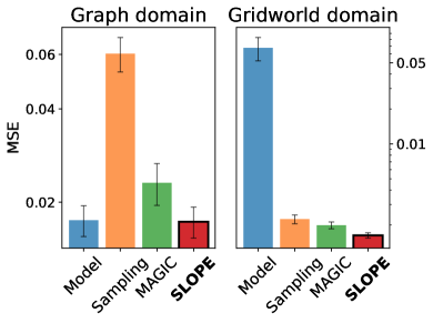
Figure 1: Representative experiments with Slope. Slope is consistently one of the best approaches, regardless of whether model-based or importance-sampling based estimators are better.

A representative experimental result for the RL setting is displayed in Figure 1. Here we consider two different domains from Voloshin et al. (2019) and compare our new estimator, Slope, with well-known baselines. Our method selects a false horizon $\eta$, uses an unbiased importance sampling approach up to horizon $\eta$, and then prematurely terminates the episode with a value estimate from a parametric estimator (in this case trained via Fitted Q iteration). Model selection focuses on choosing the false horizon $\eta$, which yields parametric and trajectory-wise importance sampling estimators as special cases (“Model” and “sampling” in the figure). Our experiments show that regardless of which of these approaches dominates, Slope is competitive with the best approach. Moreover, it outperforms Magic, the only other tuning procedure for this setting. Section 5 contains more details and experiments.

At a technical level, the fundamental challenge with estimator selection is that there is no unbiased and low-variance approach for comparing parameter choices. This precludes the use of cross validation and related approaches, as estimating the error of a method is itself an off-policy evaluation problem! Instead, adapting ideas from nonparametric statistics (Lepski and Spokoiny, 1997; Mathé, 2006), our selection procedure circumvents this error estimation problem by only using variance estimates, which are easy to obtain. At a high level, we use confidence bands for each estimator around their (biased) expectation to find one that approximately balances bias and variance. This balancing corresponds to the oracle choice, and so we obtain our performance guarantee.

Related work.

As mentioned, off-policy evaluation is a vibrant research area with contributions from machine learning, econometrics, and statistics communities. Two settings of particular interest are contextual bandits and general RL. For the former, recent and classical references include Horvitz and Thompson (1952); Dudík et al. (2014); Hirano et al. (2003); Farajtabar et al. (2018); Su et al. (2020). For the latter, please refer to Voloshin et al. (2019).

Parameter tuning is quite important for many off-policy evaluation methods. Munos et al. (2016) observe that methods like Retrace are fairly sensitive to the hyperparameter. Similarly conclusions can be drawn from the experiments of Su et al. (2019) in the contextual bandits context. Yet, when tuning is required, most works resort to heuristics. For example, in Kallus and Zhou (2018), a bandwidth hyperparameter is selected by performing an auxiliary nonparametric estimation task, while in Liu et al. (2018), it is selected as the median of the distances between points. In both cases, no theoretical guarantees are provided for such methods.

Indeed, despite the prevalence of hyperparameters in these methods, we are only aware of two methods for estimator selection: the Magic estimator (Thomas and Brunskill, 2016), and the bound minimization approach studied by Su et al. (2020) (see also Wang et al. (2017)). Both approaches use MSE surrogates for estimator selection, where Magic under-estimates the MSE and the latter uses an over-estimate. The guarantees for both methods (asymptotic consistency, competitive with unbiased approaches) are much weaker than our oracle inequality, and Slope substantially outperforms Magic in experiments.

Our approach is based on Lepski’s principle for bandwidth selection in nonparametric statistics (Lepski, 1992; Lepskii, 1991, 1993; Lepski and Spokoiny, 1997). In this seminal work, Lepski studied nonparametric estimation problems and developed a data-dependent bandwidth selection procedure that achieves optimal adaptive guarantees, in settings where procedures like cross validation do not apply (e.g., estimating a regression function at a single given point). Since its introduction, Lepski’s methodology has been applied to other statistics problems Birgé (2001); Mathé (2006); Goldenshluger and Lepski (2011); Kpotufe and Garg (2013); Page and Grünewälder (2018), but its use in machine learning has been limited. To our knowledge, Lepski’s principle has not been used for off-policy evaluation, which is our focus.

2 Setup

We formulate the estimator selection problem generically, where there is an abstract space $\mathcal{Z}$ and a distribution $\mathcal{D}$ over $\mathcal{Z}$. We would like to estimate some parameter $\theta^{\star}:=\theta(\mathcal{D})\in\mathbb{R}$, where $\theta$ is some known real-valued functional, given access to $z_{1},\ldots,z_{n}\stackrel{{\scriptstyle{iid}}}{{\sim}}\mathcal{D}$. Let $\hat{\mathcal{D}}$ denote the empirical measure, that is the uniform measure over the points $z_{1:n}$.

To estimate $\theta^{\star}$ we use a finite set of $M$ estimators $\{\theta_{i}\}_{i=1}^{M}$, where each $\theta_{i}:\Delta(\mathcal{Z})\to\mathbb{R}$. Given the dataset, we form the estimates $\hat{\theta}_{i}:=\theta_{i}(\hat{\mathcal{D}})$. Ideally, we would choose the index that minimizes the absolute error with $\theta^{\star}$, that is $\mathop{\mathrm{argmin}}_{i\in[M]}\left|\hat{\theta}_{i}-\theta^{\star}\right|$. Of course this oracle index depends on the unknown parameter $\theta^{\star}$, so it cannot be computed from the data. Instead we seek a data-driven approach for selecting an index $\hat{i}$ that approximately minimizes the error.

To fix ideas, in the RL context, we may think of $\theta$ as the value of a target policy $\pi_{\mathrm{T}}$ and $z_{1:n}$ as $n$ trajectories collected by some logging policy $\pi_{\mathrm{L}}$. The estimators $\{\theta_{i}\}_{i=1}^{M}$ may be partial importance weighting estimators Thomas and Brunskill (2016), that account for policy mismatch on trajectory prefixes of different length. These estimators modulate a bias variance tradeoff: importance weighting short prefixes will have high bias but low variance, while importance weighting the entire trajectory will be unbiased but have high variance. We will develop this example in detail in Section 5.

For performance guarantees, we decompose the absolute error into two terms: the bias and the deviation. For this decomposition, define $\bar{\theta}_{i}:=\mathbb{E}[\theta_{i}(\hat{D})]$ where the expectation is over the random samples $z_{1:n}$. Then we have

$$\left|\hat{\theta}_{i}-\theta^{\star}\right|\leq\left|\bar{\theta}_{i}-\theta^{\star}\right|+\left|\hat{\theta}_{i}-\bar{\theta}_{i}\right|=:\textsc{bias}(i)+\textsc{dev}(i).$$

As $\textsc{dev}(i)$ involves statistical fluctuations only, it is amenable to concentration arguments, so we will assume access to a high probability upper bound. Namely, our procedure uses a confidence function cnf that satisfies $\textsc{dev}(i)\leq\textsc{cnf}(i)$ for all $i\in[M]$ with high probability. On the other hand, estimating the bias is much more challenging, so we do not assume that the estimator has access to $\textsc{bias}(i)$ or any sharp upper bound. Our goal is to select an index $\hat{i}$ achieving an oracle inequality of the form

$$\left|\hat{\theta}_{\hat{i}}-\theta^{\star}\right|\leq\textsc{const}\times\min_{i}\left\{\textsc{b}(i)+\textsc{cnf}(i)\right\},$$ (1)

that holds with high probability where const is a universal constant and $\textsc{b}(i)$ is a sharp upper bound on $\textsc{bias}(i)$. This guarantee certifies that the selected estimator is competitive with the error bound for the best estimator under consideration.

We remark that the above guarantee is qualitatively similar, but weaker than the ideal guarantee of competing with the actual error of the best estimator (as opposed to the error bound). In theory, this difference is negligible as the two guarantees typically yield the same statistical conclusions in terms of convergence rates. Empirically we will see that  (1) does yield strong practical performance.

3 General Development

To obtain an oracle inequality of the form in (1), we require some benign assumptions. When we turn to the case studies, we will verify that these assumptions hold for our estimators.

Validity and Monotonicity.

The first basic property on the bias and confidence functions is that they are valid in the sense that they actually upper bound the corresponding terms in the error decomposition.

Assumption 1 (Validity).

We assume

1. (Bias Validity) $\left|\bar{\theta}_{i}-\theta^{\star}\right|\leq\textsc{b}(i)$ for all $i$.

2. (Confidence Validity) With probability at least $1-\delta$, $|\hat{\theta}_{i}-\bar{\theta}_{i}|\leq\textsc{cnf}(i)$ for all $i$.

Typically cnf can be constructed using straightforward concentration arguments such as Bernstein’s inequality. Importantly, cnf does not have to account for the bias, so the term dev that we must control is centered. We also note that cnf need not be deterministic, for example it can be derived from empirical Bernstein inequalities. We emphasize again that the estimator does not have access to $\textsc{b}(i)$.

We also require a monotonicity property on these functions.

Assumption 2 (Monotonicity).

We assume that there exists a constant $\kappa>0$ such that for all $i\in[M-1]$

1. $\textsc{b}(i)\leq\textsc{b}(i+1)$.

2. $\kappa\cdot\textsc{cnf}(i)\leq\textsc{cnf}(i+1)\leq\textsc{cnf}(i)$.

In words, the estimators should be ordered so that the bias is monotonically increasing and the confidence is decreasing but not too quickly, as parameterized by the constant $\kappa$. This structure is quite natural when estimators navigate a bias-variance tradeoff: when an estimator has low bias it typically also has high variance and vice versa. It is also straightforward to enforce a decay rate for cnf by selecting the parameter set appropriately. We will see how to do this in our case studies.

The Slope procedure.

Slope is an acronym for “Selection by Lepski’s principle for Off-Policy Evaluation.” As the name suggests, the approach is based on Lepski’s principle Lepski and Spokoiny (1997) and is defined as follows. We first define intervals

$$I(i):=[\hat{\theta}_{i}-2\textsc{cnf}(i),\hat{\theta}_{i}+2\textsc{cnf}(i)],$$

and we then use the intersection of these intervals to select an index $\hat{i}$. Specifically, the index we select is

$$\hat{i}:=\max\left\{i\in[M]:\cap_{j=1}^{i}I(j)\neq\emptyset\right\}.$$

In words, we select the largest index such that the intersection of all previous intervals is non-empty. See Figure 2 for an illustration.

Figure 2: Illustration of Slope with $M=5$. As $\cap_{i=1}^{3}I(i)$ is non-empty but $I(4)$ does not intersect with $I(3)$, we select $\hat{i}=3$.

The intuition is to adopt an optimistic view of the bias function $\textsc{b}(i)$. First observe that if $\textsc{b}(i)=0$ then, by Assumption 1, we must have $\theta^{\star}\in I(i)$. Reasoning optimistically, it is possible that we have $\textsc{b}(i)=0$ for all $i\leq\hat{i}$, since by the definition of $\hat{i}$ there exists a choice of $\theta^{\star}$ that is consistent with all intervals. As $\textsc{cnf}(\hat{i})$ is the smallest among these, index $\hat{i}$ intuitively has lower error than all previous indices. On the other hand, it is not possible to have $\textsc{b}(\hat{i}+1)=0$, since there is no consistent choice for $\theta^{\star}$ and the bias is monotonically increasing. In fact, if $\theta^{\star}\in I_{\hat{i}}$, then we must actually have $\textsc{b}(\hat{i}+1)\geq\textsc{cnf}(\hat{i}+1)$, since the intervals have width $4\textsc{cnf}(\cdot)$. Finally, since $\textsc{cnf}(\cdot)$ does not shrink too quickly, all subsequent indices cannot be much better than $\hat{i}$, the index we select. Of course, we may not have $\theta^{\star}\in I_{\hat{i}}$, so this argument does not constitute a proof of correctness, which is deferred to Appendix A.

Theoretical analysis.

We now state the main guarantee.

Theorem 3.

Under Assumption 1 and Assumption 2, we have that with probability at least $1-\delta$:

$$\left|\hat{\theta}_{\hat{i}}-\theta^{\star}\right| \leq 6(1+\kappa^{-1})\min_{i}\left\{\textsc{b}(i)+\textsc{cnf}(i)\right\}.$$

The theorem verifies that the index $\hat{i}$ satisfies an oracle inequality as in (1), with $\textsc{const}=6(1+\kappa^{-1})$. This is the best guarantee one could hope for, up to the constant factor and the caveat that we are competing with the error bound instead of the error, which we have already discussed. For off-policy evaluation, we are not aware of any other approaches that achieve any form of oracle inequality. The closest comparison is the bound minimization approach of Su et al. (2020), which is provably competitive only with unbiased indices (with $\textsc{b}(i)=0$). However in finite sample, these indices could have high variance and consequently worse performance than some biased estimator. In this sense, the Slope guarantee is much stronger.

While our main result gives a high probability absolute error bound, it is common in the off-policy evaluation literature to instead provide bounds on the mean squared error. Via a simple translation from the high-probability guarantee, we can obtain a MSE bound here as well. For this result, we use the notation $\textsc{cnf}(i;\delta)$ to highlight the fact that the confidence bounds hold with probability $1-\delta$.

Corollary 4 (MSE bound).

In addition to Assumption 1 and Assumption 2, assume that $\theta^{\star},\hat{\theta}_{i}\in[0,R]$ a.s., $\forall i$, and that cnf is deterministic. Then for any $\delta>0$,

$$\mathbb{E}(\hat{\theta}_{\hat{i}}-\theta^{\star})^{2}\leq\nicefrac{{C}}{{\kappa^{2}}}\min_{i}\left\{\textsc{b}(i)^{2}+\textsc{cnf}(i;\delta)^{2}\right\}+R^{2}\delta,$$

where $C>0$ is a universal constant.

We state this bound for completeness but remark that it is typically loose in constant factors because it is proven through a high probability guarantee. In particular, we typically require $\textsc{cnf}(i)>\sqrt{\textsc{var}(i)}$ to satisfy Assumption 1, which is already loose in comparison with a more direct MSE bound. Unfortunately, Lepski’s principle cannot provide direct MSE bounds without estimating the MSE itself, which is precisely the problem we would like to avoid. On the other hand, the high probability guarantee provided by Theorem 3 is typically more practically meaningful.

4 Application 1: continuous contextual bandits

For our first application, we consider a contextual bandit setting with continuous action space, following Kallus and Zhou (2018). Let $\mathcal{X}$ be a context space and $\mathcal{A}=[0,1]$ be a univariate real-valued action space. There is a distribution $\mathcal{P}$ over context-reward pairs, which is supported on $(\mathcal{X},\mathcal{A}\to[0,1])$. We have a stochastic logging policy $\pi_{\mathrm{L}}:\mathcal{X}\to\Delta(\mathcal{A})$ which induces the distribution $\mathcal{D}$ by generating tuples $\{(x_{i},a_{i},r_{i}(a_{i}),\pi_{\mathrm{L}}(a_{i}))\}_{i=1}^{n}$, where $(x_{i},r_{i})\sim\mathcal{P}$, $a_{i}\sim\pi_{\mathrm{L}}(x_{i})$, only $r_{i}(a_{i})$ is observed, and $\pi_{\mathrm{L}}(a_{i})$ denotes the density value. This is a bandit setting as the distribution $\mathcal{P}$ specifies rewards for all actions, but only the reward for the chosen action is available for estimation.

For off-policy evaluation, we would like to estimate the value of some target policy $\pi_{\mathrm{T}}$, which is given by $V(\pi_{\mathrm{T}}):=\mathbb{E}_{(x,r)\sim\mathcal{P},a\sim\pi_{\mathrm{T}}(x)}\left[r(a)\right]$. Of course, we do not have sample access to $\mathcal{P}$ and must resort to the logged tuples generated by $\pi_{\mathrm{L}}$. A standard off-policy estimator in this setting is

$$\hat{V}_{h}(\pi_{\mathrm{T}}):=\frac{1}{nh}\sum_{i=1}^{n}\frac{K(|\pi_{\mathrm{T}}(x_{i})-a_{i}|/h)r_{i}(a_{i})}{\pi_{\mathrm{L}}(a_{i})},$$

where $K:\mathbb{R}_{+}\to\mathbb{R}$ is a kernel function (e.g., the boxcar kernel $K(u)=\frac{1}{2}{\bf 1}\{u\leq 1\}$). This estimator has appeared in recent work (Kallus and Zhou, 2018; Krishnamurthy et al., 2019). The key parameter is the bandwidth $h$, which modulates a bias-variance tradeoff, where smaller bandwidths have lower bias but higher variance.

4.1 Theory

For a simplified exposition, we instantiate our general framework when (1) $\pi_{\mathrm{L}}$ is the uniform logging policy, (2) $K$ is the boxcar kernel, and (3) we assume that $\pi_{\mathrm{T}}(x)\in[\gamma_{0},1-\gamma_{0}]$ for all $x$. These simplifying assumptions help clarify the results, but they are not fundamentally limiting.

Fix $\gamma\in(0,1)$ and let $\mathcal{H}:=\{\gamma_{0}\gamma^{M-i}:1\leq i\leq M\}$ denote a geometrically spaced grid of $M$ bandwidth values. Let $\hat{\theta}_{i}:=\hat{V}_{h_{i}}(\pi_{\mathrm{T}})$. For the confidence term, in Appendix A, we show that we can set

$$\textsc{cnf}(i):=\sqrt{\frac{2\log(2M/\delta)}{nh_{i}}}+\frac{2\log(2M/\delta)}{3nh_{i}}$$ (2)

and this satisfies Assumption 1. With this form, it is not hard to see that the second part of Assumption 2 is also satisfied, and so we obtain the following result.

Theorem 5.

Consider the setting above with uniform $\pi_{\mathrm{L}}$, boxcar kernel, and $\mathcal{H}$ as defined above. Let b be any valid and monotone bias function, and define cnf as in (2). Then Assumption 1 and Assumption 2 are satisfied with $\kappa=\gamma$, so the guarantee in Theorem 3 applies.

In particular, if $\gamma,\gamma_{0}$ are constants and rewards are $L$-Lipschitz, for $\omega(\sqrt{\log(\log(n))/n})\leq L\leq O(n)$, then

$$\left|\hat{\theta}_{\hat{i}}-\theta^{\star}\right|\leq O\left(\left(\frac{L\log(\log(n)/\delta)}{n}\right)^{1/3}\right)$$

with probability at least $1-\delta$, without knowledge of the Lipschitz constant $L$.

For the second statement, we remark that if the Lipschitz constant were known, the best error rate achievable is $O((L\log(1/\delta)/n)^{1/3})$. Thus, Slope incurs almost no price for adaptation. We also note that it is typically impossible to know this parameter in practice.

It is technical but not difficult to derive a more general result, relaxing many of the simplifying assumptions we have made. To this end, we provide a guarantee for non-uniform $\pi_{\mathrm{L}}$ in the appendix. We do not pursue other extensions here, as the necessary techniques are well-understood (c.f., Kallus and Zhou (2018); Krishnamurthy et al. (2019)).

4.2 Experiments

We empirically evaluate using Slope for bandwidth selection in a synthetic environment for continuous action contextual bandits. We summarize the experiments and findings here with detailed description in Appendix B.

Reward fn $\in\{\textrm{quadratic, absolute value}\}$
Lipschitz const $\in\{0.1,0.3,1,3,10\}$
Kernel $\in\{\textrm{boxcar, Epanechnikov}\}$
$\pi_{\mathrm{T}}\in\{\textrm{linear, tree}\}$
$\pi_{\mathrm{L}}\in\{\textrm{linear, tree}\}$
Randomization $\in\{\textrm{unif, friendly, adversarial}\}$
Samples $\in\{10^{i}:i\in\{1,2,3,4,5\}\}$

Table 1: Contextual Bandit experiment conditions.

The environment.

We use a highly configurable synthetic environment, which allows for action spaces of arbitrary dimension, varying reward function, reward smoothness, kernel, target, and logging policies. In our experiments, we focus on $\mathcal{A}=[0,1]$. We vary all other parameters, as summarized in Table 1.

The simulator prespecifies a mapping $x\mapsto a^{\star}(x)$ which is the global maxima for the reward function. We train deterministic policies by regressing from the context to this global maxima. For the logging policy, we use two “softening” approaches for randomization, following Farajtabar et al. (2018). We use two regression models (linear, decision tree), and two softenings in addition to uniform logging, for a total of 5 logging and 2 target policies.

Methods.

We consider 7 different choices of geometrically spaced bandwidths $\mathcal{H}:=\{2^{-i}:i\in[7]\}$. We evaluate the performance of these fixed bandwidths in comparison with Slope, which selects from $\mathcal{H}$. For Slope, we simplify the implementation by replacing the confidence function in (2), with twice the empirical standard deviation of the corresponding estimate. This approximation is a valid asymptotic confidence interval and is typically sharper than (2), so we expect it to yield better practical performance. We also manually enforce monotonicity of this confidence function.

We are not aware of other viable baselines for this setting. In particular, the heuristic method of Kallus and Zhou (2018) is too computationally intensive to use at our scale.

Experiment setup.

We have 1000 conditions determined by: logging policy, target policy, reward functional form, reward smoothness, kernel, and number of samples $n$. For each condition, we first obtain a Monte Carlo estimate of the ground truth $V(\pi_{\mathrm{T}})$ by collecting 100k samples from $\pi_{\mathrm{T}}$. Then we collect $n$ trajectories from $\pi_{\mathrm{L}}$ and evaluate the squared error of each method $(\hat{V}-V(\pi_{\mathrm{T}}))^{2}$. We perform 30 replicates of each condition with different random seeds and calculate the correspond mean squared error (MSE) for each method: $\mathrm{MSE}:=\frac{1}{30}\sum_{i=1}^{30}(\hat{V}_{i}-V(\pi_{\mathrm{T}}))^{2}$ where $\hat{V}_{i}$ is the estimate on the $i^{\textrm{th}}$ replicate.

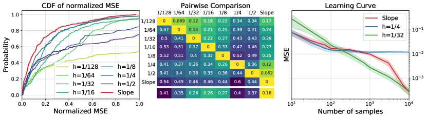
Figure 3: Experimental results for contextual bandits with continuous actions. Left: CDF of normalized MSE across all 480 conditions. Normalization is by the worst MSE for that condition. Middle: Pairwise comparison matrix, entry $P_{i,j}$ counts the fraction of conditions where method $i$ is statistically significantly better than method $j$, so larger numbers in the rows (or smaller numbers in the columns) is better. Right: asymptotic behavior of Slope selecting between two bandwidths.

Results.

The left panel of Figure 3 aggregates results via the empirical CDF of the normalized MSE, where we normalize by the worst MSE in each condition. The point $(x,y)$ indicates that on $y$-fraction of conditions the method has normalized MSE at most $x$, so better methods lie in the top-left quadrant. We see that Slope is the top performer in comparison with the fixed bandwidths.

In the center panel, we record the results of pairwise comparisons between all methods. Entry $(i,j)$ of this array is the fraction of conditions where method $i$ is significantly better than method $j$ (using a paired $t$-test with significance level $0.05$). Better methods have smaller numbers in their column, which means they are typically not significantly worse than other methods. The final row summarizes the results by averaging each column. In this aggregation, Slope also outperforms each individual fixed bandwidth, demonstrating the advantage in data-dependent estimator selection.

Finally, in the right panel, we demonstrate the behavior of Slope in a single condition as $n$ increases. Here Slope is only selecting between two bandwidths $\mathcal{H}:=\{1/4,1/32\}$. When $n$ is small, the small bandwidth has high variance but as $n$ increases, the bias of the larger bandwidth dominates. Slope effectively navigates this tradeoff, tracking $h=1/4$ when $n$ is small, and switching to $h=1/32$ as $n$ increases.

Summary.

Slope is the top performer when compared with fixed bandwidths in our experiments. This is intuitive as we do not expect a single fixed bandwidth to perform well across all conditions. On the other hand, we are not aware of other approaches for bandwidth selection in this setting, and our experiments confirm that Slope is a viable and practically effective approach.

5 Application 2: reinforcement learning

Our second application is multi-step reinforcement learning (RL). We consider episodic RL where the agent interacts with the environment in episodes of length $H$. Let $\mathcal{X}$ be a state space and $\mathcal{A}$ a finite action space. In each episode, a trajectory $\tau:=(x_{1},a_{1},r_{1},x_{2},a_{2},r_{2},\ldots,x_{H},a_{H},r_{H})$ is generated where (1) $x_{1}\in\mathcal{X}$ is drawn from a starting distribution $P_{0}$, (2) rewards $r_{h}\in\mathbb{R}$ and next state $x_{h+1}\in\mathcal{X}$ are drawn from a system descriptor $(r_{h},x_{h+1})\sim P_{+}(x_{h},a_{h})$ for each $h$ (with the obvious definition for time $H$), and (3) actions $a_{1},\ldots,a_{H}\in\mathcal{A}$ are chosen by the agent. A policy $\pi:\mathcal{X}\mapsto\Delta(\mathcal{A})$ chooses a (possibly stochastic) action in each state and has value $V(\pi):=\mathbb{E}\left[\sum_{h=1}^{H}\gamma^{h-1}r_{h}\mid a_{1:H}\sim\pi\right]$, where $\gamma\in(0,1)$ is a discount factor. For normalization, we assume that rewards are in $[0,1]$ almost surely.

Environment	GW	MC	Graph	PO-Graph
Horizon	25	250	16	16
MDP	Yes	Yes	Yes	No
Sto Env	Both	No	Yes	Yes
Sto Rew	No	No	Both	Both
Sparse Rew	No	No	Both	Both
Model class	Tabular	NN	Tabular	Tabular
Samples	$2^{7:9}$	$2^{8:10}$	$2^{7:10}$	$2^{7:10}$
# of policies	5	4	2	2

Table 2: RL Environment Details

For off-policy evaluation, we have a dataset of $n$ trajectories $\{(x_{i,1},a_{i,1},r_{i,1},\ldots,x_{i,H},a_{i,H},r_{i,H})\}_{i=1}^{n}$ generated by following some logging policy $\pi_{\mathrm{L}}$, and we would like to estimate $V(\pi_{\mathrm{T}})$ for some other target policy. The importance weighting approach is also standard here, and perhaps the simplest estimator is

$$\hat{V}_{\mathrm{IPS}}(\pi_{\mathrm{T}}):=\frac{1}{n}\sum_{i=1}^{n}\sum_{h=1}^{H}\gamma^{h-1}\rho_{i,h}r_{i,h},$$ (3)

where $\rho_{i,h}:=\prod_{h^{\prime}=1}^{h}\tfrac{\pi_{\mathrm{T}}(a_{i,h^{\prime}}\mid x_{i,h^{\prime}})}{\pi_{\mathrm{L}}(a_{i,h^{\prime}}\mid x_{i,h^{\prime}})}$ is the step-wise importance weight. This estimator is provably unbiased under very general conditions, but it suffers from high variance due to the $H$-step product of density ratios. An alternative approach is to directly model the value function using supervised learning, as in a regression based dynamic programming algorithm like Fitted Q Evaluation (Riedmiller, 2005; Szepesvári and Munos, 2005). While these “direct modeling” approaches have very low variance, they are typically highly biased because they rely on supervised learning models that cannot capture the complexity of the environment. Thus they lie on the other extreme of the bias-variance spectrum.

To navigate this tradeoff, Thomas and Brunskill (2016) propose a family of partial importance weighting estimators. To instantiate this family, we first train a direct model $\hat{V}_{\mathrm{DM}}:\mathcal{X}\times[H]\to\mathbb{R}$ to approximate $(x,h)\mapsto\mathbb{E}_{\pi}\left[\sum_{h^{\prime}=h}^{H}\gamma^{h^{\prime}-h}r_{h^{\prime}}\mid x_{h}=x\right]$, for example via Fitted Q Evaluation. Then, the estimator is

$$\hat{V}_{\eta}(\pi_{\mathrm{T}}) :=\frac{1}{n}\sum_{i=1}^{n}\sum_{h=1}^{\eta}\gamma^{h-1}\rho_{i,h}r_{i,h}+\frac{1}{n}\sum_{i=1}^{n}\gamma^{\eta}\rho_{i,\eta}\hat{V}_{\mathrm{DM}}(x_{i,\eta+1},\eta+1),$$ (4)

The estimator has a parameter $\eta$ that governs a false horizon for the importance weighting component. Specifically, we only importance weight the rewards up until time step $\eta$ and we complete the trajectory with the predictions from a direct modeling approach. The model selection question here centers around choosing the false horizon $\eta$ at which point we truncate the unbiased importance weighted estimator.

5.1 Theory

We instantiate our general estimator selection framework in this setting. Let $\hat{\theta}_{i}:=\hat{V}_{H-i+1}(\pi_{\mathrm{T}})$ for $i\in\{1,\ldots,H+1\}$. Intuitively, we expect that the variance of $\hat{\theta}_{i}$ is large for small $i$, since the estimator involves a product of many density ratios. Indeed, in the appendix, we derive a confidence bound and prove that it verifies our assumptions. The bound is quite complicated so we do not display it here, but we refer the interested reader to (7) in Appendix A. The bound is a Bernstein-type bound which incorporates both variance and range information. We bound these as

$$\textrm{Variance}(\hat{V}_{\eta}(\pi_{\mathrm{T}}))\leq 3V_{\mathrm{max}}^{2}(1+\sum_{h=1}^{\eta}\gamma^{2(h-1)}p_{\mathrm{max}}^{h}),\qquad\textrm{Range}(\hat{V}_{\eta}(\pi_{\mathrm{T}}))\leq 3V_{\mathrm{max}}(1+\sum_{h=1}^{\eta}\gamma^{h-1}p_{\mathrm{max}}^{h}),$$

where $V_{\mathrm{max}}:=(1-\gamma)^{-1}$ is the range of the value function and $p_{\mathrm{max}}:=\sup_{x,a}\tfrac{\pi_{\mathrm{T}}(a\mid x)}{\pi_{\mathrm{L}}(a\mid x)}$ is the maximum importance weight, which should be finite. Equipped with these bounds, we can apply Bernstein’s inequality to obtain a valid confidence interval. Moreover, it is not hard to show that this confidence interval is monotonic with $\kappa:=(1+\gamma p_{\mathrm{max}})^{-1}$. This yields the following theorem.

Theorem 6 (Informal).

Consider the episodic RL setting with $\hat{\theta}_{i}:=\hat{V}_{H-i+1}(\pi_{\mathrm{T}})$ defined in (4). Let b be any valid and monotone bias function. Then with $\textsc{cnf}(i)$ as in (7) in the appendix, Assumption 1 and  Assumption 2 with $\kappa:=(1+\gamma p_{\mathrm{max}})^{-1}$ hold, so Theorem 3 applies.

A more precise statement is provided in Appendix A, and we highlight some salient details here. First, our analysis actually applies to a doubly-robust variant of the estimator $\hat{V}_{\eta}$, in the spirit of (Jiang and Li, 2016). Second, $\textsc{b}(i):=\tfrac{\gamma^{H-i+1}-\gamma^{H}}{1-\gamma}$ is valid and monotone, and can be used to obtain a concrete error bound. However, the oracle inequality yields a stronger conclusion, since it applies for any valid and monotone bias function. This universality is particularly important when using the doubly robust variant, since it is typically not possible to sharply bound the bias.

The closest comparison is Magic (Thomas and Brunskill, 2016), which is strongly consistent in our setting. However, it does not satisfy any oracle inequality and is dominated by Slope in experiments.

5.2 Experiments

We evaluate Slope in RL environments spanning 106 different experimental conditions. We also compare with previously proposed estimators and assess robustness under various conditions. Our experiments closely follow the setup of Voloshin et al. (2019). Here we provide an overview of the experimental setup and highlight the salient differences from theirs. All experimental details are in Appendix C.

The environments.

We use four RL environments: Mountain Car, Gridworld, Graph, and Graph-POMDP (abbreviated MC, GW, Graph, and PO-Graph). All four environments are from Voloshin et al. (2019), and they provide a broad array of environmental conditions, varying in terms of horizon length, partial observability, stochasticity in dynamics, stochasticity in reward, reward sparsity, whether function approximation is required, and overlap between logging and target policies. Logging and target policies are from Voloshin et al. (2019). A summary of the environments and their salient characteristics is displayed in Table 2.

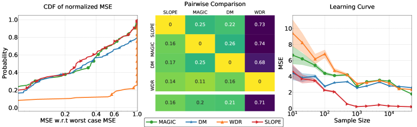
Figure 4: Left: Cumulative distribution function of the normalized MSE for all conditions, Middle: Pairwise comparison matrix $P$ for the methods, over all conditions. Element $P_{ij}$ denotes the percentage of times that method $i$ outperforms method $j$. The last row shows the column average for each method, the lower the better. Right: Learning Curve for the Hybrid domain.

Methods.

We compare four estimators: the direct model (DM), a self-normalized doubly robust estimator (WDR), (c) Magic, and (d) Slope. All four methods use the same direct model, which we train either by Fitted Q Evaluation or by $Q^{\pi}(\lambda)$ (Munos et al., 2016), following the guidelines in Voloshin et al. (2019). The doubly robust estimator is the most competitive estimator in the family of full-trajectory importance weighting. It is similar to (3), except that the direct model is used as a control variate and the normalizing constant $n$ is replaced with the sum of importance weights. Magic, as we have alluded to, is the only other estimator selection procedure we are aware of for this setting. It aggregates partial importance weighting estimators to optimize a surrogate for the MSE. For Slope, we use twice the empirical standard deviation as the confidence function, which is asymptotically valid and easier to compute.

We do not consider other baselines for two reasons. First, DM, WDR, and Magic span the broad estimator categories (importance weighted, direct, hybrid) within which essentially all estimators fall. Secondly, many other estimators have hyperparameters that must be tuned, and we believe Slope will also be beneficial when used in these contexts.

Experiment Setup.

We have 106 experimental conditions determined by environment, stochasticity of dynamics and reward, reward sparsity, logging policy, target policy, and number of trajectories $n$. For each condition, we calculate the MSE for each method by averaging over 100 replicates.

Results.

In the left panel of Figure 4, as in Section 4.2, we first visualize the aggregate results via the cumulative distribution function (CDF) of the normalized MSE in each condition (normalizing by the worst performing method in each condition). As a reminder, the figure reads as follows: for each $x$ value, the corresponding $y$ value is the fraction of conditions where the estimator has normalized MSE at most $x$. In this aggregation, we see that WDR has the worst performance, largely due to intolerably high variance. Magic and DM are competitive with each other with Magic having a slight edge. Slope appears to have the best aggregate performance; for the most part its CDF dominates the others.

In the central panel, we display an array of statistical comparisons between pairs of methods. As before, entry $(i,j)$ of this array is computed by counting the fraction of conditions where method $i$ beats $j$ in a statistically significant manner (we use paired $t$-test on the MSE with significance level $0.05$). The column-wise averages are also displayed.

In this aggregation, we see clearly that Slope dominates the three other methods. First, Slope has column average that is smaller than the other methods. More importantly, Slope is favorable when compared with each other method individually. For example, Slope is (statistically) significantly worse than Magic on 16% of the conditions, but it is significantly better on 25%. Thus, this visualization clearly demonstrates that Slope is the best performing method in aggregate across our experimental conditions.

Before turning to the final panel of Figure 4, we recall Figure 1, where we display results for two specific conditions. Here, we see that Slope outperforms or is statistically indistinguishable from the best baseline, regardless of whether direct modeling is better than importance weighting! We are not aware of any selection method that enjoys this property.

Learning curves.

The final panel of Figure 4 visualizes the performance of the four methods as the sample size increases. Here we consider the Hybrid domain from Thomas and Brunskill (2016), which is designed specifically to study the performance of partial importance weighting estimators. The domain has horizon 22, with partial observability in the first two steps, but full observability afterwards. Thus a (tabular) direct model is biased since it is not expressive enough for the first two time steps, but $\hat{V}_{2}(\pi_{\mathrm{T}})$ is a great estimator since the direct model is near-perfect afterwards.

The right panel of Figure 4 displays the MSE for each method as we vary the number of trajectories, $n$ (we perform 128 replicates and plot bars at $\pm 2$ standard errors). We see that when $n$ is small, DM dominates, but its performance does not improve as $n$ increases due to bias. Both WDR and Magic catch up as $n$ increases, but Slope is consistently competitive or better across all values of $n$, outperforming the baselines by a large margin. Indeed, this is because Slope almost always chooses the optimal false horizon index of $\eta=2$ (e.g., 90% of the replicates when $n=500$).

Summary.

Our experiments show that Slope is competitive, if not the best, off-policy evaluation procedure among Slope, Magic, DM, and WDR. We emphasize that Slope is not an estimator, but a selection procedure that in principle can select hyperparameters for many estimator families. Our experiments with the partial importance weighting family are quite convincing, and we believe this demonstrates the potential for Slope when used with other estimator families for off-policy evaluation in RL.

6 Discussion

In summary, this paper presents a new approach for estimator selection in off-policy evaluation, called Slope. The approach applies quite broadly; in particular, by appropriately spacing hyperparameters, many common estimator families can be shown to satisfy the assumptions for Slope. To demonstrate this, we provide concrete instantiations in two important applications. Our theory yields, to our knowledge, the first oracle-inequalities for off-policy evaluation in RL. Our experiments demonstrate strong empirical performance, suggesting that Slope may be useful in many off-policy evaluation contexts.

Appendix A Proofs

A.1 Proofs for Section 3

Proof of Theorem 3.

The proof is similar to that of Corollary 1 in (Mathé, 2006). Define $\tilde{i}=\max\{i:\textsc{b}(i)\leq\textsc{cnf}(i)\}$. The proof is composed of two steps: first we show that we are competitive with $\tilde{i}$ and then we show that $\tilde{i}$ is competitive with the best index.

Competing with $\tilde{i}$.

Observe that since b is monotonically increasing, and cnf is monotonically decreasing, for $i\leq\tilde{i}$ we have

$$\textsc{b}(i)\leq\textsc{b}(\tilde{i})\leq\textsc{cnf}(\tilde{i})\leq\textsc{cnf}(i).$$

Therefore, for $i\leq\tilde{i}$

$$\left|\hat{\theta}_{i}-\theta^{\star}\right|\leq\textsc{b}(i)+\textsc{cnf}(i)\leq 2\textsc{cnf}(i).$$

This implies that $\theta^{\star}\in I_{i}$ for all $i\leq\tilde{i}$.

As a consequence, the definition of our chosen index $\hat{i}$ implies that $\hat{i}\geq\tilde{i}$, which in turn implies that $I_{\tilde{i}}\cap I_{\hat{i}}\neq\emptyset$. So, there exists $x\in I_{\tilde{i}}\cap I_{\hat{i}}$ such that $|x-\hat{\theta}_{\tilde{i}}|\leq 2\textsc{cnf}(\tilde{i})$ and $|x-\hat{\theta}_{\hat{i}}|\leq 2\textsc{cnf}(\hat{i})$. As we know that $\theta^{\star}\in I_{\tilde{i}}$, we get

$$|\hat{\theta}_{\hat{i}}-\theta^{\star}|\leq|\hat{\theta}_{\hat{i}}-x|+|x-\hat{\theta}_{\tilde{i}}|+|\hat{\theta}_{\tilde{i}}-\theta^{\star}|\leq 2\textsc{cnf}(\hat{i})+2\textsc{cnf}(\tilde{i})+2\textsc{cnf}(\tilde{i})\leq 6\textsc{cnf}(\tilde{i}).$$ (5)

Comparing $\tilde{i}$ to $i^{\star}$.

Define $i^{\star}:=\mathop{\mathrm{argmin}}_{i}\{\textsc{b}(i)+\textsc{cnf}(i)\}$ which is the index we actually want to compete with in our guarantee. If we compare $\tilde{i}$ with $i^{\star}$, then by the above argument we can translate to $\hat{i}$. For this, we consider two cases:

If $i^{\star}\leq\tilde{i}$, then by definition of $\tilde{i}$, we have

$$\textsc{b}(\tilde{i})+\textsc{cnf}(\tilde{i})\leq 2\textsc{cnf}(\tilde{i})\leq 2\textsc{cnf}(i^{\star})\leq 2(\textsc{cnf}(i^{\star})+\textsc{b}(i^{\star})),$$

so we are a factor of $2$ worse.

On the other hand, if $i^{\star}>\tilde{i}$ then by Assumption 2 and the optimality condition for $\tilde{i}$

$$\kappa\textsc{cnf}(\tilde{i})\leq\textsc{cnf}(\tilde{i}+1)\leq\textsc{b}(\tilde{i}+1)\leq\textsc{b}(i^{\star}).$$

This implies

$$\textsc{b}(\tilde{i})+\textsc{cnf}(\tilde{i})\leq(1+\nicefrac{{1}}{{\kappa}})\textsc{b}(i^{\star}).$$

As $\kappa\leq 1$, this bound dominates the previous case, and together, with (5) we have

$$\left|\hat{\theta}_{\hat{i}}-\theta^{\star}\right|\leq 6\times\textsc{cnf}(\tilde{i})\leq 6(1+\nicefrac{{1}}{{\kappa}})\min_{i\in[M]}\left\{\textsc{b}(i)+\textsc{cnf}(i)\right\}.$$ ∎

Proof of Corollary 4.

For the MSE calculation, we simply need to translate from the high probability guarantee to the MSE, which is not difficult under Assumption 1. In particular, fix $\delta$ and let $\mathcal{E}$ be the event that all confidence bounds are valid, which holds with probability $1-\delta$, then we have

$$\mathbb{E}(\hat{\theta}_{\hat{i}}-\theta^{\star})^{2} =\mathbb{E}(\hat{\theta}_{\hat{i}}-\theta^{\star})^{2}{\bf 1}\left\{\mathcal{E}\right\}+\mathbb{E}(\hat{\theta}_{\hat{i}}-\theta^{\star})^{2}{\bf 1}\left\{\bar{\mathcal{E}}\right\}$$

$$\leq\mathbb{E}(\hat{\theta}_{\hat{i}}-\theta^{\star})^{2}{\bf 1}\left\{\mathcal{E}\right\}+R^{2}\delta$$

$$\leq\mathbb{E}{\bf 1}\left\{\mathcal{E}\right\}\left(6(1+\nicefrac{{1}}{{\kappa}})\mathbb{E}\min_{i\in[M]}\left\{\textsc{b}(i)+\textsc{cnf}(i;\delta)\right\}\right)^{2}+R^{2}\delta$$

$$\leq 72(1+\nicefrac{{1}}{{\kappa}})^{2}\min_{i\in[M]}\left\{\textsc{b}(i)^{2}+\textsc{cnf}(i;\delta)^{2}\right\}+R^{2}\delta.$$

Here in the first line we are introducing the event $\mathcal{E}$ and its complement. In the second, we use that $\hat{\theta}_{i},\theta^{\star}\in[0,R]$ almost surely and that $\mathbb{P}[\bar{\mathcal{E}}]\leq\delta$ according to Assumption 1. In the third line, we apply Theorem 3, which holds under event $\mathcal{E}$. The final step uses the simplification that $(a+b)^{2}\leq 2a^{2}+2b^{2}$. ∎

A.2 Proofs for Section 4

Proof of Theorem 5.

Let us first verify that the confidence function specified in (2) satisfy Assumption 1. We will apply Bernstein’s inequality, which requires variance and range bounds. For the variance, a single sample satisfies

$$\operatorname*{{\rm Var}}\left(\frac{K(|\pi_{\mathrm{T}}(x)-a|/h)r(a)}{h\times\pi_{\mathrm{L}}(a\mid x)}\right) \leq\frac{1}{h}\mathbb{E}\left[\frac{K(|\pi_{\mathrm{T}}(x)-a|/h)^{2}}{h\times\pi_{\mathrm{L}}^{2}(a\mid x)}\mid a\sim\pi_{\mathrm{L}}(\cdot\mid x)\right]\leq\frac{1}{2h},$$

where we first use that the variance is upper bounded by the second moment, and then we use that $\pi_{\mathrm{L}}$ is uniform and the boxcar kernel is at most $1/2$. Finally, we use that by a change of variables $K(\cdot/h)/h$ integrates to $1$. Note that we are using that $\pi_{\mathrm{T}}\in[\gamma_{0},1-\gamma_{0}]$, as we are integrating over the support of $\pi_{\mathrm{L}}$.

For the range, we have

$$\sup\frac{K(|\pi_{\mathrm{T}}(x)-a|/h)r(a)}{h\times\pi_{\mathrm{L}}(a\mid x)}\leq\frac{1}{2h}.$$

Therefore, Bernstein’s inequality gives that with probability $1-\delta$ we have

$$\left|\hat{V}_{h}(\pi_{\mathrm{T}})-\mathbb{E}\hat{V}_{h}(\pi_{\mathrm{T}})\right|\leq\sqrt{\frac{\log(2/\delta)}{nh}}+\frac{\log(2/\delta)}{3nh},$$

and the first claim follows by a union bound.

Monotonicity is also easy to verify with this definition of cnf. In particular, since $h_{i}=\gamma h_{i+1}$ and $\gamma<1$, we immediately have that

$$\gamma\textsc{cnf}(i)=\gamma\sqrt{\frac{\log(2M/\delta)}{nh_{i}}}+\gamma\frac{\log(2M/\delta)}{3nh_{i}}=\gamma\sqrt{\frac{\log(2M/\delta)}{n\gamma h_{i+1}}}+\frac{\log(2M/\delta)}{3nh_{i+1}}\leq\textsc{cnf}(i+1)$$

Clearly $\textsc{cnf}(i+1)\leq\textsc{cnf}(i)$, and so Assumption 2 holds. This verifies that we may apply Theorem 3.

For the last claim, if the rewards are $L$-Lipschitz, then we claim we can set $\textsc{b}(i)=Lh_{i}$. To see why, observe that

$$\left|\mathbb{E}V_{h}(\pi_{\mathrm{T}})-V(\pi_{\mathrm{T}})\right| =\left|\mathbb{E}_{(x,r),a\sim\pi_{\mathrm{L}}(x)}\frac{K(|\pi_{\mathrm{T}}(x)-a|/h)r(a)}{h}-r(\pi_{\mathrm{T}}(x))\right|$$

$$=\left|\mathbb{E}_{(x,r)}\int_{a^{\prime}}\frac{{\bf 1}\left\{|\pi_{\mathrm{T}}(x)-a|\leq h\right\}r(a)}{2h}-r(\pi_{\mathrm{T}}(x))\right|$$

$$=\left|\mathbb{E}_{(x,r)}\int_{a^{\prime}}\frac{{\bf 1}\left\{|\pi_{\mathrm{T}}(x)-a|\leq h\right\}(r(a)-r(\pi_{\mathrm{T}}(x)))}{2h}\right|\leq Lh.$$

Clearly this bias bound is monotonic. To apply Theorem 3, it is better to first simplify the confidence function. Observe that as $\theta^{\star},\bar{\theta}_{i}\in[0,1]$, it is always better to clip the estimates $\hat{\theta}_{i}$ to lie in $[0,1]$. This has no bearing on the bias and only improves the deviation term, and in particular allows us to replace $\textsc{cnf}(i)$ with $\min\{\textsc{cnf}(i),1\}$. This leads to a further simplification:

$$\sqrt{\frac{\log(2M/\delta)}{nh_{i}}}+\frac{\log(2M/\delta)}{3nh_{i}}\leq 1\Rightarrow\sqrt{\frac{\log(2M/\delta)}{nh_{i}}}+\frac{\log(2M/\delta)}{3nh_{i}}\leq\frac{4}{3}\sqrt{\frac{\log(2M/\delta)}{nh_{i}}}$$

Therefore we may replace cnf with this latter function and by Theorem 3 we guarantee that with probability at least $1-\delta$

$$\left|\hat{\theta}_{\hat{i}}-\theta^{\star}\right|\leq 6(1+\gamma^{-1})\min_{i}\left\{Lh_{i}+\frac{4}{3}\sqrt{\frac{\log(2M/\delta)}{nh_{i}}}\right\}.$$

The optimal choice for $h$ is $h^{\star}:=\left(\frac{4}{3L}\sqrt{\frac{\log(2M/\delta)}{n}}\right)^{2/3}$, which will in general not be in our set $\mathcal{H}$. However, if we use this choice for $h$, the error rate is $O((L/n)^{1/3})$, and since we know that $\theta^{\star}\in[0,1]$, if $L>n$ then this error guarantee is trivial. In other words, the maximum value of $L$ that we are interested in adapting to is $L_{\max}=n$. This will be useful in setting the number of models to search over $M$.

To set $M$, we want to ensure that there exists some $h_{i}$ such that $h_{i}\leq h^{\star}\leq h_{i+1}$. We first verify the first inequality, which requires that

$$\gamma_{0}\gamma^{M}\leq h^{\star}:=\left(\frac{4}{3L}\sqrt{\frac{\log(2M/\delta)}{n}}\right)^{2/3}$$

We will always take $M\geq 2$, which implies that $\log(2M/\delta)\geq 1$. Then, since we are only interested in $L\leq n$, a sufficient condition here is

$$\gamma_{0}\gamma^{M}\leq\frac{4}{3}^{2/3}n^{-1}\Rightarrow M\geq\frac{C_{\gamma_{0}}\log(n)}{\log(1/\gamma_{0})},$$

where $C_{\gamma_{0}}$ is a constant that only depends on $\gamma_{0}$. The upper bound $h^{\star}\leq h_{i+1}$ is satisfied as soon as $n$ is large enough, provided that $L\geq\omega(\sqrt{\log(\log(n))/n})$, which we are assuming. Thus we know that there is $i^{\star}$ such that $h_{i^{\star}}\leq h^{\star}\leq h_{i^{\star}}/\gamma$, and using this choice, we have

$$\left|\hat{\theta}_{\hat{i}}-\theta^{\star}\right| \leq 6(1+\gamma^{-1})\left\{Lh_{i^{\star}}+\frac{4}{3}\sqrt{\frac{\log(2M/\delta)}{nh_{i^{\star}}}}\right\}\leq 6(1+\gamma^{-1})\left\{Lh^{\star}+\frac{4}{3}\sqrt{\frac{\log(2M/\delta)}{\gamma nh^{\star}}}\right\}$$

$$\leq 6(1+\gamma^{-1})\cdot\frac{c_{1}}{\sqrt{\gamma}}(L\log(2M/\delta)/n)^{1/3}\leq C_{\gamma,\gamma_{0}}(L\log(\log(n)/\delta)/n)^{1/3},$$

where $C_{\gamma,\gamma_{0}}$ is a constant that depends only on $\gamma,\gamma_{0}$. ∎

Note that if $\pi_{\mathrm{L}}$ is non-uniform, but satisfies $\inf_{x,a}\pi_{\mathrm{L}}(a\mid x)\geq p_{\mathrm{min}}$, then very similar arguments apply. In particular, we have that both variance and range are bounded by $\frac{1}{2hp_{\mathrm{min}}}$, and some Bernstein’s inequality in this case yields

$$\left|\hat{V}_{h}(\pi_{\mathrm{T}})-\mathbb{E}\hat{V}_{h}(\pi_{\mathrm{T}})\right|\leq\sqrt{\frac{\log(2/\delta)}{nhp_{\mathrm{min}}}}+\frac{\log(2/\delta)}{3nhp_{\mathrm{min}}},$$

Monotonicity follows from the same calculation as before and the clipping trick yields a more interpretable final bound, which holds with probability at least $1-\delta$, of

$$\left|\hat{\theta}_{\hat{i}}-\theta^{\star}\right|\leq 6(1+\gamma^{-1})\min_{i}\left\{Lh_{i}+\frac{4}{3}\sqrt{\frac{\log(2M/\delta)}{nh_{i}p_{\mathrm{min}}}}\right\}.$$

The remaining calculation for $M$ is analogous, since this bound is identical to the previous one with $n$ replaced by $np_{\mathrm{min}}$. Thus, we obtain a final bound of $C_{\gamma,\gamma_{0}}(L\log(\log(n/\delta))/(np_{\mathrm{min}}))^{1/3}$.

A.3 Proofs for Section 5

We first develop and state the more precise version of Theorem 6. We introduce the doubly robust version of the partial importance weighting estimator. As it is the empirical average over $n$ trajectories, here we will focus on a single trajectory $(x_{1},a_{1},r_{1},\ldots,x_{H},a_{H},r_{H})$ sampled by following the logging policy $\pi_{\mathrm{L}}$.

Define $\hat{V}_{\mathrm{DR}}^{0}:=0$ and

$$\hat{V}_{\mathrm{DR}}^{H+1-h}:=\hat{V}(x_{h})+p_{h}(r_{h}+\gamma\hat{V}_{\mathrm{DR}}^{H-t}-\hat{Q}(x_{h},a_{h})),\qquad p_{h}:=\frac{\pi_{\mathrm{T}}(a_{h}\mid x_{h})}{\pi_{\mathrm{L}}(a_{h}\mid x_{h})}.$$

where $\hat{Q}$ is the direct model, trained via supervised learning, and $\hat{V}(x)=\mathbb{E}_{a\sim\pi_{\mathrm{T}}(x)}\hat{Q}(x,a)$. The full horizon doubly-robust estimator is $\hat{V}_{\mathrm{DR}}:=\hat{V}_{\mathrm{DR}}^{H}$. To define the $\eta$-step partial estimator, let $\hat{V}_{\mathrm{DM}}^{\eta}:=\rho_{\eta}\hat{Q}(x_{\eta+1},\pi_{\mathrm{T}}(x_{\eta+1}))$, which is an estimate of $\mathbb{E}_{\pi_{\mathrm{T}}}\left[V(x_{\eta+1})\right]$. Set $\hat{V}_{\mathrm{DM}}^{H}:=0$. Then for a false horizon $\eta$, we define a similar recursion

$$\hat{V}^{H+1-h}_{\eta}:=\left\{\begin{aligned} \hat{V}(x_{h})+p_{h}(r_{h}+\gamma V_{\eta}^{H-h}-\hat{Q}(x_{h},a_{h}))&\textrm{ if }1\leq h<\eta\\ \hat{V}(x_{h})+p_{h}(r_{h}+\gamma\hat{V}_{\mathrm{DM}}^{\eta}-\hat{Q}(x_{h},a_{h}))&\textrm{ if }h=\eta.\end{aligned}\right.$$

The doubly robust variant of the $\eta$-step partial importance weighted estimator is $\hat{V}_{\eta}^{H}$. We also define $\hat{V}_{0}^{H}=\hat{V}_{\mathrm{DM}}^{0}$ which estimates $\mathbb{E}\left[V(x_{1})\right]$. Observe that if in the definition of $\hat{V}_{\mathrm{DR}}$, we take $\hat{V},\hat{Q}\equiv 0$ then we obtain the estimator in (4).

Define $\Delta:=\log(2(H+1)/\delta)$, $V_{\mathrm{max}}:=(1-\gamma)^{-1}$ and recall that $p_{\mathrm{max}}:=\max_{x,a}\tfrac{\pi_{\mathrm{T}}(a|x)}{\pi_{\mathrm{L}}(a|x)}$. Then define

$$\textsc{b}(i) :=\frac{\gamma^{H-i+1}-1}{1-\gamma}$$

$$\textsc{cnf}(i) :=\sqrt{\frac{6V_{\mathrm{max}}^{2}\left(1+\sum_{h=1}^{H-i+1}\gamma^{2(h-1)}p_{\mathrm{max}}^{h}\right)\Delta}{n}}+\frac{6V_{\mathrm{max}}\left(1+\sum_{h=1}^{H-i+1}\gamma^{h-1}p_{\mathrm{max}}^{h}\right)\Delta}{3n}$$

With these definitions, we know state the theorem

Theorem 7 (Formal version of Theorem 6).

In the episodic reinforcement learning setting with discount factor $\gamma$, consider the doubly robust partial importance weighting estimators $\hat{\theta}_{i}:=\hat{V}^{H}_{H-i+1}(\pi_{\mathrm{T}})$ for $i\in\{1,\ldots,H+1\}$. Then b and cnf are valid and monotone, with $\kappa:=(1+\gamma p_{\mathrm{max}})^{-1}$.

Proof of Theorem 7.

We now turn to the proof.

Bias analysis.

By repeatedly applying the tower property, the expectation for $\hat{V}_{\eta}^{H}$ is

$$\mathbb{E}\left[\hat{V}_{\eta}^{H}\right] =\mathbb{E}_{\pi_{\mathrm{L}}}\left[\hat{V}(x_{1})+p_{1}(r_{1}+\gamma\hat{V}_{\eta}^{H-1}-\hat{Q}(x_{1},a_{1})\right]$$

$$=\mathbb{E}_{x_{1}}\left[\hat{V}(x_{1})+\mathbb{E}_{a_{1}\sim\pi_{\mathrm{L}}(x_{1}),a_{2:H}\sim\pi_{\mathrm{L}}}\left[p_{1}(r_{1}+\gamma\hat{V}_{\eta}^{H-1}-\hat{Q}(x_{1},a_{1}))\mid x_{1}\right]\right]$$

$$=\mathbb{E}_{x_{1}}\left[\hat{V}(x_{1})+\mathbb{E}_{a_{1}\sim\pi_{\mathrm{T}}(x_{1}),a_{2:H}\sim\pi_{\mathrm{L}}}\left[r_{1}+\gamma\hat{V}_{\eta}^{H-1}-\hat{Q}(x_{1},a_{1})\mid x_{1}\right]\right]$$

$$=\mathbb{E}_{x_{1},a_{1}\sim\pi_{\mathrm{T}}(x_{1})}[r]+\gamma\mathbb{E}_{x_{2}\sim\pi_{\mathrm{T}},a_{2:H}\sim\pi_{\mathrm{L}}}\left[\hat{V}_{\eta}^{H-1}\right]$$

$$=...$$

$$=\mathbb{E}_{\pi_{\mathrm{T}}}\left[\sum_{h=1}^{\eta}\gamma^{h-1}r\right]+\gamma^{\eta}\mathbb{E}_{x_{\eta+1}\sim\pi_{\mathrm{T}}}\left[\hat{V}_{\mathrm{DM}}^{\eta}\right].$$

Here, we use that $p_{1}$ is the one-step importance weight, so it changes the action distribution from $\pi_{\mathrm{L}}$ to $\pi_{\mathrm{T}}$. We also use the relationship between the direct models $\hat{Q}$ and $\hat{V}$. Therefore, the bias is

$$\left|\mathbb{E}\left[\hat{V}_{\eta}^{H}\right]-V(\pi_{\mathrm{T}})\right|=\gamma^{\eta}\left|\hat{V}_{\mathrm{DM}}^{\eta}-\mathbb{E}_{\pi_{\mathrm{T}}}\left[V(x_{\eta+1})\right]\right|\leq\frac{\gamma^{\eta}-\gamma^{H}}{1-\gamma}=:\textsc{b}(H-\eta+1)$$ (6)

The first identity justifies are choice of $\hat{V}_{\mathrm{DM}}^{\eta}$ which attempts to minimize this bias using the direct model. The inequality here follows from the fact that rewards are in $[0,1]$, which implies that values at time $\eta+1$ are in $\left[0,\frac{1-\gamma^{H-\eta}}{1-\gamma}\right]$. As $\gamma\in(0,1)$, clearly we have that $\textsc{b}(i)$ is monotonically increasing with $i$ increasing. Thus this bias bound is valid.

Variance analysis.

For the variance calculation, let $\mathbb{E}_{h}\left[\cdot\right],\operatorname*{{\rm Var}}_{h}(\cdot)$ denote expectation and variance conditional on all randomness before time step $h$. Adapting Theorem 1 of Jiang and Li (2016) the variance for $1\leq h<\eta$ is given by the recursive formula:

$$\operatorname*{{\rm Var}}_{h}(\hat{V}_{\eta}^{H+1-h}) =\operatorname*{{\rm Var}}_{h}(\mathbb{E}\left[\hat{V}_{\eta}^{H+1-h}\mid x_{h}\right])+\mathbb{E}_{h}\left[\operatorname*{{\rm Var}}(p_{h}\Delta(x_{h},a_{h})\mid x_{h})\right]$$

$$~{}~{}~{}~{}~{}~{}+\mathbb{E}_{h}\left[p_{h}^{2}\operatorname*{{\rm Var}}(r_{h})\right]+\mathbb{E}_{h}\left[\gamma^{2}p_{h}^{2}\operatorname*{{\rm Var}}_{h+1}(\hat{V}_{\eta}^{H-h})\right],$$

where $\Delta(x_{h},a_{h}):=\hat{Q}(x_{h},a_{h})-Q(x_{h},a_{h})$. For $h=\eta$ it is identical, except that in the last term we use $\hat{V}_{\mathrm{DM}}^{\eta}$ instead of $\hat{V}_{\eta}^{H-\eta}$ (which is not defined).

Unrolling the recursion, the full expression for the variance is

$$\operatorname*{{\rm Var}}(\hat{V}_{\eta}^{H}) =\sum_{h=1}^{\eta}\mathbb{E}\left[\gamma^{2(h-1)}\rho^{2}_{h-1}\operatorname*{{\rm Var}}_{h}(\mathbb{E}\left[\hat{V}_{\eta}^{H+1-h}\mid x_{h}\right])\right]$$

$$+\sum_{h=1}^{\eta}\mathbb{E}\left[\gamma^{2(h-1)}\rho^{2}_{h-1}\mathbb{E}_{h}\left[\operatorname*{{\rm Var}}(p_{h}\Delta(x_{h},a_{h})\mid x_{h})\right]\right]$$

$$+\sum_{h=1}^{\eta}\mathbb{E}\left[\gamma^{2(h-1)}\rho^{2}_{h-1}\mathbb{E}_{h}\left[p_{h}^{2}\operatorname*{{\rm Var}}(r_{h})\right]\right]$$

$$+\mathbb{E}\left[\gamma^{2\eta}\rho_{\eta}^{2}\operatorname*{{\rm Var}}_{\eta+1}(\hat{V}_{\mathrm{DM}}^{\eta})\right].$$

For the variance bound, we do not attempt to obtain the sharpest bound possible. Instead, we use the following facts: (1) rewards are in $[0,1]$, (2) all values, value estimates, and $Q$ are at most $(1-\gamma)^{-1}=:V_{\mathrm{max}}$, and (3) for a random variable $X$ that is bounded by $B$ almost surely, we have $\operatorname*{{\rm Var}}(X)\leq B^{2}$. Using these facts in each term gives

$$\operatorname*{{\rm Var}}(\hat{V}_{\eta}^{H}) \leq\sum_{h=1}^{\eta}\mathbb{E}\left[\gamma^{2(h-1)}\rho^{2}_{h-1}V_{\mathrm{max}}^{2}\right]+\sum_{h=1}^{\eta}\mathbb{E}\left[\gamma^{2(h-1)}\rho_{h}^{2}V_{\mathrm{max}}^{2}\right]+\sum_{h=1}^{\eta}\mathbb{E}\left[\gamma^{2(h-1)}\rho^{2}_{h}\right]+\mathbb{E}\left[\gamma^{2\eta}\rho_{\eta}^{2}V_{\mathrm{max}}^{2}\right]$$

$$=\sum_{h=1}^{\eta+1}\mathbb{E}\left[\gamma^{2(h-1)}\rho_{h-1}^{2}V_{\mathrm{max}}^{2}\right]+\sum_{h=1}^{\eta}\mathbb{E}\left[\gamma^{2(h-1)}\rho_{h}^{2}(V_{\mathrm{max}}^{2}+1)\right]$$

$$\leq 3V_{\mathrm{max}}^{2}\sum_{h=1}^{\eta}\mathbb{E}\left[\gamma^{2(h-1)}\rho_{h}^{2}\right]+V_{\mathrm{max}}^{2}$$

Here in the first line we use the three facts we stated above. In the second line we collect the terms. In the third line we note that $\gamma^{2(h-1)}\rho_{h-1}^{2}\leq\gamma^{2(h-2)}\rho_{h-1}^{2}$ since $\gamma\in(0,1)$, so we can re-index the first summation and group terms again.

To simplify further, let $p_{\mathrm{max}}:=\sup_{x,a}\frac{\pi_{\mathrm{T}}(a\mid x)}{\pi_{\mathrm{L}}(a\mid x)}$ denote the largest importance weight and note that as $\mathbb{E}_{h}[p_{h}]=1$, we have

$$\sum_{h=1}^{\eta}\mathbb{E}\left[\gamma^{2(h-1)}\rho_{h}^{2}\right]\leq\sum_{h=1}^{\eta}\mathbb{E}\left[\gamma^{2(h-1)}p_{\mathrm{max}}\rho_{h-1}^{2}\mathbb{E}_{h}[w_{h}]\right]\leq\ldots\leq\sum_{h=1}^{\eta}\gamma^{2(h-1)}p_{\mathrm{max}}^{h}.$$

Therefore, our variance bound will be

$$\operatorname*{{\rm Var}}(\hat{V}_{\eta}^{H})\leq 3V_{\mathrm{max}}^{2}\left(1+\sum_{h=1}^{\eta}\gamma^{2(h-1)}p_{\mathrm{max}}^{h}\right).$$

For the range, we obtain the recursion (for $1\leq h<\eta$):

$$\left|\hat{V}_{\eta}^{H+1-h}\right|\leq V_{\mathrm{max}}+p_{\mathrm{max}}(1+V_{\mathrm{max}})+p_{\mathrm{max}}\gamma\left|\hat{V}_{\eta}^{H-h}\right|,$$

with the terminal condition $\left|\hat{V}_{\mathrm{DM}}^{\eta}\right|\leq V_{\mathrm{max}}$. A somewhat crude upper bound is

$$\left|\hat{V}_{\eta}^{H}\right|\leq 3V_{\mathrm{max}}\left(1+\sum_{h=1}^{\eta}\gamma^{h-1}p_{\mathrm{max}}^{h}\right),$$

which has a similar form to the variance expression.

Therefore, Bernstein’s inequality reveals that with probability $1-\delta$, we have that the $n$-trajectory empirical averages satisfy

$$\left|\hat{V}_{\eta}^{H}-\mathbb{E}\hat{V}_{\eta}^{H}\right|\leq\sqrt{\frac{6V_{\mathrm{max}}^{2}\left(1+\sum_{h=1}^{\eta}\gamma^{2(h-1)}p_{\mathrm{max}}^{h}\right)\log(2/\delta)}{n}}+\frac{6V_{\mathrm{max}}\left(1+\sum_{h=1}^{\eta}\gamma^{h-1}p_{\mathrm{max}}^{h}\right)\log(2/\delta)}{3n}.$$ (7)

This bound is clearly seen to be montonically increasing in $\eta$, which is montonically decreasing with $i$ as required. The reason is that when we increase $\eta$ we add one additional non-negative term to both the variance and range expressions.

Finally, we must verify that the bound does not decrease too quickly. For this, we first verify the following elementary fact

Fact 8.

Let $z\geq 0$ and $t\geq 0$ then

$$\frac{1+\sum_{\tau=1}^{t}z^{\tau}}{1+\sum_{\tau=1}^{t-1}z^{\tau}}\leq 1+z.$$

Proof.

Using the geometric series formula, we can rewrite

$$\frac{1+\sum_{\tau=1}^{t}z^{\tau}}{1+\sum_{\tau=1}^{t-1}z^{\tau}}=1+\frac{z^{t}}{1+\sum_{\tau=1}^{t-1}z^{\tau}}\leq 1+z.$$ ∎

Using the above fact, we can see that the variance bound decreases at rate $(1+\gamma^{2}p_{\mathrm{max}})$ and the range bound decreases at rate $(1+\gamma p_{\mathrm{max}})$. The range bound dominates here, since

$$\sqrt{1+\gamma^{2}p_{\mathrm{max}}}\leq\sqrt{1+\gamma^{2}p_{\mathrm{max}}^{2}}\leq 1+\gamma p_{\mathrm{max}}$$

Therefore, we may take the decay constant to be $1/(1+\gamma p_{\mathrm{max}})$ to verify Assumption 2. ∎

Appendix B Details for continuous contextual bandits experiments

B.1 The simulation environment.

Here, we explain some of the important details of the simulation environment. The simulator is initialized with a $d_{x}$ dimensional context space and action space $[0,1]^{d}$ for some parameter $d$. For our experiments we simply take $d=1$. There is also a hidden parameter matrix $\beta^{\star}\sim\mathcal{N}(0,I)$ with $\beta^{\star}\in\mathbb{R}^{d\times d_{x}}$. In each round, contexts are sampled iid from $\mathcal{N}(0,I)$, then the optimal action $a^{\star}(x):=\sigma(\beta^{\star}x)$, where $\sigma(z)=\tfrac{e^{z}}{e^{z}+1}$ is the standard sigmoid, and the function is applied component-wise. This optimal action $a^{\star}$ is used in the design of the reward functions.

We consider two different reward functions called “absolute value” and “quadratic.” The first is simply $\ell(a):=1-\min(L\left\|a-a^{\star}(x)\right\|_{1},1)$, while the latter is $\ell(a):=1-\min(L/4\sum_{j=1}^{d}(a_{j}-a^{\star}_{j}(x))^{2},1)$. Here $L$ is the Lipschitz constant, which is also a configurable.

For policies, the uniform logging policy simply chooses $a\sim\textrm{Unif}([0,1]^{d})$ on each round. Other logging and target policies are trained via regression on 10 vector-valued regression samples $(x,a^{\star}(x)+\mathcal{N}(0,0.5\cdot I))$ where $x\sim\mathcal{N}(0,I)$. We use two different regression models: linear + sigmoid implemented in PyTorch, and a decision tree implemented in scikit-learn. Both regression procedures yield deterministic policies, and in our experiments we take this policies to be $\pi_{\mathrm{T}}$.

For $\pi_{\mathrm{L}}$ we implement two softening techniques following Farajtabar et al. (2018), called “friendly” and “adversarial,” and both techniques take two parameters $\alpha,\beta$. Both methods are defined for discrete action spaces, and to adapt to the continuous setting we partition the continuous action space into $m$ bins (for one-dimensional spaces). We round the deterministic action chosen by the regression model to its associated bin, run the softening procedure to choose a (potentially different) bin, and then sample an action uniformly from this bin. For higher dimensional action spaces, we discretize each dimension individually, so the softening results in a product measure.

Friendly softening with discrete actions is implemented as follows. We sample $U\sim\textrm{Unif}([-0.5,0.5])$ and then the updated action is $\pi_{\textrm{det,disc}}(x)$ with probability $\alpha+\beta U$ and it is uniform over the remaining discrete actions with the remaining probability. Here $\pi_{\textrm{det,disc}}$ is the deterministic policy obtained by the regression model, discretized to one of the $m$ bins. Adversarial softening instead is uniform over all discrete actions with probability $1-(\alpha+\beta U)$ and it is uniform over all but $\pi_{\textrm{det,disc}}(x)$ with the remaining probability. In both cases, once we have a discrete action, we sample a continuous action from the corresponding bin.

The simulator also supports two different kernel functions: Epanechnikov and boxcar. The boxcar kernel is given by $K(u)=\frac{1}{2}{\bf 1}\{\left|u\right|\leq 1\}$, while Epanechnikov is $K(u)=0.75\cdot(1-u^{2}){\bf 1}\{\left|u\right|\leq 1\}$. We address boundary bias by normalizing the kernel appropriately, as opposed to forcing the target policy to choose actions in the interior. This issue is also discussed in Kallus and Zhou (2018).

Finally, we also vary the number of logged samples and the Lipschitz constant of the loss functions.

B.2 Reproducibility Checklist

Data collection process. All data are synthetically generated as described above.

Dataset and Simulation Environment. We will make the simulation environment publicly available.

Excluded Data. No excluded data.

Training/Validation/Testing allocation. There is no training/validation/testing setup in off policy evaluation. Instead all logged data are used for evaluation.

Hyper-parameters. Hyperparameters used in the experimental conditions are: $n\in 10^{1:5}$, $h\in\{2^{-(1:7)}$, $L\in\{0.1,0.3,1,3,10\}$, in addition to the other configurable parameters (e.g., softening technique, kernel, logging policy, target policy).

Evaluation runs. There are 1000 conditions, each with 30 replicates with different random seeds.

Description of experiments. For each condition, determined by logging policy, softening technique, target policy, sample size, lipschitz constant, reward function, and kernel type, we generate $n$ logged samples following $\pi_{\mathrm{L}}$, and 100k samples from $\pi_{\mathrm{T}}$ to estimate the ground truth $V(\pi_{\mathrm{T}})$. All fixed-bandwidth estimators and Slope are calculated based on the same logged data. The MSE is estimated by averaging across the 30 replicates, each with different random seed.

For the learning curve in the right panel of Figure 3 the specific condition shown is: uniform logging policy, linear+sigmoid target policy, $L=3$, absolute value reward, boxcar kernel. MSE estimates are measured at $n=\{1,3,7\}\times 10^{1:3}\cup\{10,000\}$. We perform 100 replicates for this experiment.

Measure and Statistics. Results are shown in Figure 3. Statistics are based on empirical CDF calculated by aggregating the 1000 conditions. Typically there are no error bars for such plots. Pairwise comparison is based on paired $t$-test over all pair of methods and conditions, with significance level $0.05$. The learning curve is based on 100 replicates, with error bar corresponding to $\pm 2$ standard errors shown in the plots.

Computing infrastructure. Experiments were run on Microsoft Azure.

Appendix C Details for reinforcement learning experiments

C.1 Experiment Details

Environment Description. We provide brief environment description below. More details can be found in Thomas and Brunskill (2016); Voloshin et al. (2019); Brockman et al. (2016).

• Mountain car is a classical benchmark from OpenAI Gym. We make the same modification as Voloshin et al. (2019). The domain has 2-dimensional state space (position and velocity) and one-dimensional action $\{\textrm{left,nothing,right}\}$. The reward is $r=-1$ for each timestep before reaching the goal. The initial state has position uniformly distributed in the discrete set $\{-0.4,-0.5,-0.6\}$ with velocity $0$. The horizon is set to be $H=250$ and there is an absorbing state at $(0.5,0)$. The domain has deterministic dynamics, as well as deterministic, dense reward.

• Graph and Graph-POMDP are adopted from Voloshin et al. (2019). The Graph domain has horizon 16, state space $\{0,1,2,\cdots,31\}$ and action space $\{0,1\}$. The initial state is $x_{0}=0$, and we have the state-independent stochastic transition model with $\mathbb{P}(x_{t+1}=2t+1|a=0)=0.75$, $\mathbb{P}(x_{t+1}=2t+2|a=0)=0.25$, $\mathbb{P}(x_{t+1}=2t+1|a=1)=0.25$, $\mathbb{P}(x_{t+1}=2t+2|a=1)=0.75$. In the dense reward configuration, we have $r(x_{t},a_{t},x_{t+1})=2(x_{t+1}\mod 2)-1$ $\forall t\leq T$. The sparse reward setting has $r(x_{t},a_{t},x_{t+1})=0$ $\forall t<T-1$ with reward only at the last time step, according to the dense reward function. We also consider a stochastic reward setting, where we change the reward to be $r(x_{t},a_{t},x_{t+1})\sim\mathcal{N}(2(x_{t+1}\mod 2)-1,1)$. Graph-POMDP is a modified version of Graph where states are grouped into 6 groups. Only the group information is observed, so the states are aliased.

• Gridworld is also from Voloshin et al. (2019). The state space is an $8\times 8$ grid with four actions [up, down, left, right]. The initial state distribution is uniform over the left column and top row, while the goal is in the bottom right corner. The horizon length is 25. The states belongs to four categories: Field, Hole, Goal, Others. The reward at Field is -0.005, Hole is -0.5, Goal is 1 and Others is -0.01. The exact map can be found in Voloshin et al. (2019).

• Hybrid Domain is from Thomas and Brunskill (2016). It is a composition of two other domains from the same study, called ModelWin and ModelFail. The ModelFail domain has horizon 2, four states $\{s_{0},s_{1},s_{2},s_{a}\}$ and two actions $\{0,1\}$. The agent starts at $s_{0}$, goes to $s_{1}$ with reward 1 if $a=0$, and goes to $s_{2}$ with reward if $a=1$. Then it transitions to the absorbing state $s_{a}$. This environment has partial observability so that $\{s_{0},s_{1},s_{2}\}$ are aliased together.

  In the hybrid domain the absorbing state $s_{a}$ is replaced with a new state $s_{1}$ in the ModelWin domain. This domain has four states $\{s_{1},s_{2},s_{3},s_{a}\}$. The action space is $\{0,1\}$. The agent starts from $s_{1}$. Upon taking action $a=0$, it goes to $s_{2}$ with probability 0.6 and receives reward 1, and goes to $s_{3}$ with probability 0.4 and reward -1. If $a=1$, it does the opposite. From $s_{2}$ and $s_{3}$ the agent deterministically transitions to $s_{1}$ with 0 reward. do a deterministic transition back to $s_{1}$ with 0 reward. The horizon here is 20 and $x_{20}=s_{a}$. The states are fully observable.

Models.

Instead of experiment with all possible approaches for direct modeling, which is quite burdensome, we follow the high-level guidelines provided in Table 3 of Voloshin et al. (2019)’s paper: for Graph, PO-Graph, and Mountain Car we use FQE because these environments are stochastic and have severe mismatch between logging and target policy. In contrast, Gridworld has moderate policy mismatch, so we use $Q^{\pi}(\lambda)$. For the Hybrid domain, we use a simple maximum-likelihood approximate model to predict the full transition operator and rewards, and plan in the model to estimate the value function.

Policy.

For Gridworld and Mountain Car, we use $\epsilon$-Greedy polices as logging and target policies. To derive these, we first train a base policy using value iteration and then we take $\pi(a^{\star}|x)=1-\epsilon$ and $\pi(a\mid x)=\epsilon/(|\mathcal{A}|-1)$ for $a\neq a^{\star}(x)$, where $a^{\star}(x)=\mathop{\mathrm{argmax}}\hat{Q}(x,a)$ for the learned $\hat{Q}$ function. In Gridworld, we take the following policy pairs: $[(1,0.1),(0.6,0.1),(0.2,0.1),(0.1,0.2),(0.1,0.6)]$, where the first argument is the $\epsilon$ parameter for . For Mountain Car domain, we take the following policy pairs: $[(0.1,0),(1,0),(1,0.1),(0.1,1)]$ where the first argument is the parameter for $\pi_{\mathrm{L}}$ and the second is for $\pi_{\mathrm{T}}$. For the Graph and Graph-POMDP domain, both logging and target policies are static polices with probability $p$ going left (marked as $a=0$) and probability $1-p$ going right (marked as $a=1$), i.e., $\pi(a=0|x)=p$ and $\pi(a=1|x)=1-p$ $\forall x$. In both environments, we vary $p$ of the logging policy to be $0.2$ and $0.6$, while setting $p$ for target policy to be $0.8$. For the Hybrid domain, we use the same policy as Thomas and Brunskill (2016). For the first ModelFail part, $\pi_{\mathrm{L}}(a=0)=0.88$ and $\pi_{\mathrm{L}}(a=1)=0.12$, while the target policy does the opposite. For the second ModelWin part, $\pi_{\mathrm{L}}(a=0|s_{1})=0.73$ and $\pi_{\mathrm{L}}(a=1|s_{1})=0.27$, and the target policy does the opposite. For both policies, they select actions uniformly when $s\in\{s_{2},s_{3}\}$.

Other parameters.

For both the Graph and Graph-POMDP, we use $\gamma=0.98$ and $N\in 2^{7:10}$. For Gridworld, $\gamma=0.99$ and $N\in 2^{7:9}$. For Mountain Car, $\gamma=0.96$ and $N\in 2^{8:10}$. For Hybrid, $\gamma=0.99$ and $N\in\{10,20,50,\cdots,10000,20000,50000\}$. Each condition is averaged over 100 replicates.

C.2 Reproducibility Checklist

Data collection process. All data are synthetically generated as described above.

Dataset and Simulation Environment. The Mountain Car environment is downloadable from OpenAI (Brockman et al., 2016). Graph, Graph-POMDP, Gridworld, and the Hybrid domain are available at https://github.com/clvoloshin/OPE-tools, which is the supporting code for Voloshin et al. (2019).

Excluded Data. No excluded data.

Training/Validation/Testing allocation. There is no training/validation/testing setup in off policy evaluation. Instead all logged data are used for evaluation.

Hyper-parameters. Hyperparameters (apart from those optimized by Slope) are optimized followng the guidelines of Voloshin et al. (2019). For MountainCar, the direct model is trained using a 2-layer fully connected neural network with hidden units 64 and 32. The batch size is 32 and convergence is set to be $1e-4$, network weights are initialized with truncated Normal$(0,0.1)$. For tabular models, convergence of Graph and Graph-POMDP is $1e-5$ and Gridworld is $4e-4$.

Evaluation runs. All conditions have 100 replicates with different random seeds.

Description of experiments. For each condition, determined by the choice of environment, stochastic/deterministic reward, sparse/dense reward, stochastic/deterministic transition model, logging policy $\pi_{\mathrm{L}}$, target policy $\pi_{\mathrm{T}}$ and sample size $N$. We generate $N$ logged trajectories following $\pi_{\mathrm{L}}$, and 10000 samples from $\pi_{\mathrm{T}}$ to compute the ground truth $V(\pi_{\mathrm{T}})$. All baselines and Slope are calculated based on the same logged data. The MSE is estimated by averaging across the 100 replicates, each with different random seed.

Measure and Statistics. Results are shown in Figure 4. Statistics are based on empirical CDF calculated by aggregating the 106 conditions. Typically there are no error bars in ECDF plots. Pairwise comparison is based on paired $t$-test over all pair of methods over all conditions. Each test has significance level $0.05$. Learning curve is based on Hybrid domain with 128 replicates, with error bar corresponding to $\pm 2$ standard errors shown in the plots.

Computing infrastructure. RL experiments were conducted in a Linux compute cluster.

References

- Birgé (2001) Lucien Birgé. An alternative point of view on lepski’s method. Lecture Notes-Monograph Series, 2001.
- Bradtke and Barto (1996) Steven J Bradtke and Andrew G Barto. Linear least-squares algorithms for temporal difference learning. Machine learning, 1996.
- Brockman et al. (2016) Greg Brockman, Vicki Cheung, Ludwig Pettersson, Jonas Schneider, John Schulman, Jie Tang, and Wojciech Zaremba. Openai gym. arXiv:1606.01540, 2016.
- Dudík et al. (2014) Miroslav Dudík, Dumitru Erhan, John Langford, and Lihong Li. Doubly robust policy evaluation and optimization. Statistical Science, 2014.
- Farajtabar et al. (2018) Mehrdad Farajtabar, Yinlam Chow, and Mohammad Ghavamzadeh. More robust doubly robust off-policy evaluation. In International Conference on Machine Learning, 2018.
- Goldenshluger and Lepski (2011) Alexander Goldenshluger and Oleg V Lepski. Bandwidth selection in kernel density estimation: oracle inequalities and adaptive minimax optimality. The Annals of Statistics, 2011.
- Hirano et al. (2003) Keisuke Hirano, Guido W Imbens, and Geert Ridder. Efficient estimation of average treatment effects using the estimated propensity score. Econometrica, 2003.
- Horvitz and Thompson (1952) Daniel G Horvitz and Donovan J Thompson. A generalization of sampling without replacement from a finite universe. Journal of the American Statistical Association, 1952.
- Jiang and Li (2016) Nan Jiang and Lihong Li. Doubly robust off-policy value evaluation for reinforcement learning. In International Conference on Machine Learning, 2016.
- Kallus and Zhou (2018) Nathan Kallus and Angela Zhou. Policy evaluation and optimization with continuous treatments. In Artificial Intelligence and Statistics, 2018.
- Kpotufe and Garg (2013) Samory Kpotufe and Vikas Garg. Adaptivity to local smoothness and dimension in kernel regression. In Advances in Neural Information Processing Systems, 2013.
- Krishnamurthy et al. (2019) Akshay Krishnamurthy, John Langford, Aleksandrs Slivkins, and Chicheng Zhang. Contextual bandits with continuous actions: Smoothing, zooming, and adapting. In Conference on Learning Theory, 2019.
- Lepski (1992) Oleg V Lepski. Asymptotically minimax adaptive estimation. i: Upper bounds. optimally adaptive estimates. Theory of Probability & Its Applications, 1992.
- Lepski and Spokoiny (1997) Oleg V Lepski and Vladimir G Spokoiny. Optimal pointwise adaptive methods in nonparametric estimation. The Annals of Statistics, 1997.
- Lepskii (1991) Oleg V Lepskii. On a problem of adaptive estimation in gaussian white noise. Theory of Probability & Its Applications, 1991.
- Lepskii (1993) Oleg V Lepskii. Asymptotically minimax adaptive estimation. ii. schemes without optimal adaptation: Adaptive estimators. Theory of Probability & Its Applications, 1993.
- Liu et al. (2018) Qiang Liu, Lihong Li, Ziyang Tang, and Dengyong Zhou. Breaking the curse of horizon: Infinite-horizon off-policy estimation. In Advances in Neural Information Processing Systems, 2018.
- Mathé (2006) Peter Mathé. The lepskii principle revisited. Inverse problems, 2006.
- Munos et al. (2016) Rémi Munos, Tom Stepleton, Anna Harutyunyan, and Marc Bellemare. Safe and efficient off-policy reinforcement learning. In Advances in Neural Information Processing Systems, 2016.
- Page and Grünewälder (2018) Stephen Page and Steffen Grünewälder. The goldenshluger-lepski method for constrained least-squares estimators over RKHSs. arXiv:1811.01061, 2018.
- Precup et al. (2000) Doina Precup, Richard S Sutton, and Satinder Singh. Eligibility traces for off-policy policy evaluation. In International Conference on Machine Learning, 2000.
- Riedmiller (2005) Martin Riedmiller. Neural fitted q iteration–first experiences with a data efficient neural reinforcement learning method. In European Conference on Machine Learning, 2005.
- Su et al. (2019) Yi Su, Lequn Wang, Michele Santacatterina, and Thorsten Joachims. Cab: Continuous adaptive blending for policy evaluation and learning. In International Conference on Machine Learning, 2019.
- Su et al. (2020) Yi Su, Maria Dimakopoulou, Akshay Krishnamurthy, and Miroslav Dudík. Doubly robust off-policy evaluation with shrinkage. In International Conference on Machine Learning, 2020.
- Sutton (1988) Richard S Sutton. Learning to predict by the methods of temporal differences. Machine learning, 1988.
- Swaminathan et al. (2017) Adith Swaminathan, Akshay Krishnamurthy, Alekh Agarwal, Miro Dudik, John Langford, Damien Jose, and Imed Zitouni. Off-policy evaluation for slate recommendation. In Advances in Neural Information Processing Systems, 2017.
- Szepesvári and Munos (2005) Csaba Szepesvári and Rémi Munos. Finite time bounds for sampling based fitted value iteration. In International Conference on Machine Learning, 2005.
- Thomas and Brunskill (2016) Philip Thomas and Emma Brunskill. Data-efficient off-policy policy evaluation for reinforcement learning. In International Conference on Machine Learning, 2016.
- Voloshin et al. (2019) Cameron Voloshin, Hoang M Le, Nan Jiang, and Yisong Yue. Empirical study of off-policy policy evaluation for reinforcement learning. arXiv:1911.06854, 2019.
- Wang et al. (2017) Yu-Xiang Wang, Alekh Agarwal, and Miroslav Dudik. Optimal and adaptive off-policy evaluation in contextual bandits. In International Conference on Machine Learning, 2017.