Gradient-Based Adversarial Training on Transformer Networks for Detecting Check-Worthy Factual Claims

Abstract.

We present a study on the efficacy of adversarial training on transformer neural network models, with respect to the task of detecting check-worthy claims. In this work, we introduce the first adversarially-regularized, transformer-based claim spotter model that achieves state-of-the-art results on multiple challenging benchmarks. We obtain a $4.70$ point F1-score improvement over current state-of-the-art models on the ClaimBuster Dataset and CLEF2019 Dataset, respectively. In the process, we propose a method to apply adversarial training to transformer models, which has the potential to be generalized to many similar text classification tasks. Along with our results, we are releasing our codebase and manually labeled datasets. We also showcase our models’ real world usage via a live public API. footnote 14

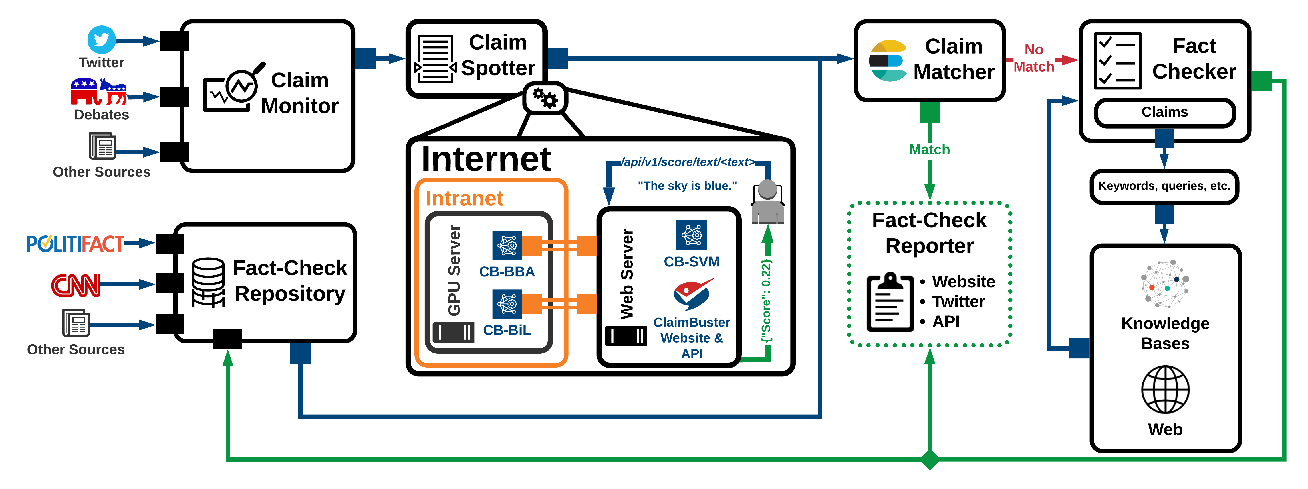
Figure 1. A Diagram of Our Current Fact-Checking Framework

1. Introduction

The creation and propagation of misinformation has become an increasingly important issue for our society to tackle. Today, many falsehoods are spread via mediums that allow quick dissemination of information, including social media, news outlets, and televised programs. The distribution of objectively incorrect information can negatively impact the operation of our society in many spheres. Especially in the realm of political discourse, misinformation can shake public confidence in government institutions,  erroneously inform political judgements (Allcott and Gentzkow, 2017), and reinforce confidence in wrong information (Chan et al., 2017).

In recent years, the number of fact-checking outlets has grown from 44 in 2014 to 226 in 2019  as part of a global movement to suppress misinformation. These outlets, including PolitiFact,  Snopes,  and FactCheck.org,  hire human fact-checkers to perform claim-checking, a process in which they vet factual claims by reviewing relevant source documents and interviewing subject experts. In addition to outlets that directly fact-check claims, there exist many projects that use computing to aid fact-checkers in disseminating information to the general public, including Schema.org’s ClaimReview  which organizes fact-checks into a unified database; FactStream  which compiles fact-checks into a smartphone application; and Fatima,  a bot built by Aos Fatos, a Brazilian fact-checking organization, that scans Twitter for tweets containing already-debunked misinformation and refers readers to relevant fact-checks. These organizations and projects play a central role in fighting misinformation, as fact-checks are effective not only for debunking false claims but also deterring speakers from making false claims in the future (Nyhan and Reifler, 2015).

However, due to the intense time commitment demanded by fact-checking, combined with the rapid rate at which new content surfaces via modern media channels, many problematic claims go unnoticed and unchecked (Pennycook and Rand, 2019). These challenges present an opportunity for automated fact-checking tools to help fact-checkers perform their duties. There are several prominent fact-checking projects that are currently testing automated systems, including FactChecker  which queries knowledge bases, cross-references known fact-checks, and provides custom ranked Google search results; ClaimPortal   which uses ClaimBuster (Hassan et al., 2017b; Jimenez and Li, 2018; Hassan et al., 2017a, 2015) to select tweets that are worth fact-checking, as well as various algorithms to retrieve relevant articles and pre-existing fact-checks (Majithia et al., 2019); Squash  which fact-checks live debates by converting speech to text and querying a database of pre-existing fact-checks; Fakta  which checks claims against reliable web sources (Nadeem et al., 2019); and FullFact  which is developing systems to cluster groups of similar claims together.

Claim-spotting is a process that precedes claim-checking where check-worthy claims are spotted from large streams of information available from various sources (e.g., newscasts, news websites, Twitter, Facebook). Claim-spotting is an area that is highly suitable for machine learning algorithms to tackle. The work presented here focuses on the claim-spotting component of ClaimBuster,  which scores claims based on their check-worthiness. This is paramount to ensuring that 1) check-worthy factual claims are not missed by fact-checkers and 2) unimportant or non-factual claims do not congest fact-checkers’ intellectual bandwidth. To this day, ClaimBuster’s API is regularly in use not only by internal projects such as ClaimPortal but also external collaborators such as the Duke Reporters’ Lab. The closest projects to ClaimBuster in this space are QCRI’s ClaimRank  project, and a component in FullFact’s proposed automated fact-checking system which they gave the name Hawk in their whitepaper.  QCRI’s ClaimRank is very similar to ClaimBuster in that it ranks claims by assigning them a check-worthiness score from $0$ to $1$. As for Hawk and FullFact’s system, not many details have been released.

Currently, no existing claim-spotter (Hassan et al., 2017a, 2015; Jimenez and Li, 2018; Hansen et al., 2019; Favano et al., 2019) has attempted to apply transformers (Vaswani et al., 2017) to the claim-spotting task. The transformer is a new deep learning architecture that has recently allowed for rapid progress and development in the natural language processing field. Particularly, Bidirectional Encoding Representations from Transformers (BERT) (Devlin et al., 2019) has achieved state-of-the-art performance on many challenging language understanding and classification benchmarks. We surmise that BERT’s architecture is suited for our claim-spotting task. However, BERT models have upwards of 300 million trainable parameters, making them highly susceptible to overfitting (Caruana et al., 2001), especially on limited amounts of training data. To address this, we propose to incorporate adversarial training into a BERT-based model as a regularization technique. Gradient-based adversarial training (Goodfellow et al., 2014; Miyato et al., 2016, 2018) is a procedure that trains classifiers to be resistant to small, approximately worst-case perturbations to its inputs. It was first applied to computer vision tasks in (Goodfellow et al., 2014) and later brought to the NLP domain in Long Short-Term Memory Networks (Hochreiter and Schmidhuber, 1997) by Goodfellow et al. (Miyato et al., 2016, 2018). No prior work has attempted to incorporate this type of adversarial training into transformer networks. We are the first to propose this technique, which is also potentially applicable in many other NLP-related tasks.

Motivated by the above, we introduce the first adversarially-regularized, transformer-based claim-spotting model that achieves state-of-the-art results on challenging claim-spotting benchmarks. Our contributions are summarized as follows:

• We are the first to apply gradient-based adversarial training to transformer networks.

• We present the first transformer-based neural network architecture for claim-spotting.

• Our models are the first claim-spotters to be regularized by gradient-based adversarial training.

• Our models achieve state-of-the-art performance by a substantial margin on challenging claim-spotting benchmarks.

• We release a public codebase, dataset, and API for both reproducibility and further development (Section 7).

2. ClaimBuster Overview

In this section we present a brief history and overview on the ClaimBuster project. We cover its inception and impact in the community, as well as the current status of our fact-checking framework.

2.1. ClaimBuster’s History and Current Status

ClaimBuster’s foundation was first established in (Hassan et al., 2015), where Hassan et. al. first presented results on different machine learning models trained on an early version of the dataset we are using currently. This work later evolved into what is currently known as ClaimBuster and was presented in (Hassan et al., 2017a; Hassan et al., 2017b). Since then, ClaimBuster has partnered with the Duke Reporters’ Lab (DRL)  and collaborated with them through ClaimBuster’s API. During this time ClaimBuster’s API has been called over $\mathbf{47,000,000}$ times by internal projects and over $\mathbf{456,000}$ times by the DRL. ClaimPortal is the internal project that has made the most use of the ClaimBuster API. It scores tweets and provides relevant fact-checks for tweets using the claim-matching component seen in Figure 1. Through this project we have seen that we can successfully apply ClaimBuster to different domains, such as Twitter. As for the DRL, they generate and send out a daily e-mail to fact-checkers with the latest top claims that were identified by ClaimBuster from television and social media. Through our collaboration with the DRL we have been able to contribute to which claims are fact-checked by major news outlets.  The accessibility of our work has allowed it, in general, to have a widespread impact in the fact-checking community.

Since the development of the original SVM model, we have been exploring deep learning (Jimenez and Li, 2018) approaches to improve our claim-spotting model. Recently, this culminated with us employing the BERT architecture due to BERT and its derivative models’ proven track record in performing well on NLP related tasks such as SQuAD and GLUE.   Since then, we have also re-evaluated our approach to the classes used within our datasets, how our dataset is generated, and refined our overall process when it comes to evaluating models. This turnaround in our approach to our dataset has come after a lengthy evaluation of our extraction criteria (i.e., what we consider high-quality labels), and the ratio of check-worthy to non-check-worthy sentences in the dataset. Through these evaluations, we are confident we have obtained a better quality dataset than that used in previous works. The work presented here will also begin a thorough test period with our collaborators at the DRL.

2.2. Fact-Checking Framework

Figure 1 showcases the current status of our fact-checking framework. We monitor claims from various sources (e.g., Twitter, political debates, etc.), and we are even able to process live television closed-caption feeds for important events such as presidential debates. ClaimSpotter then handles scoring all of the claims that our claim monitoring system captures. ClaimSpotter is accessible to the public via an API, which only requires a free API key  to access. We are deploying the deep learning models for the public and other researchers to test and verify the models presented in this paper. Each deep-learning model is running off of a dedicated Nvidia GTX 1080Ti. All resources are running on the same network, so there is no significant overhead added by a server to server communication.

In addition, we also have a repository of fact-checked claims which we use in conjunction with ElasticSearch  in our claim-matcher component to verify the veracity of any claims that have been previously fact-checked by professional fact-checkers. If no previous fact-checks are found then we can send these claims to our fact-checking component, which is still being developed. Currently, our approach is to convert claims to questions (Heilman, 2011) in order to query knowledge bases (e.g., Wolfram, Google, etc.) using natural language to see if they can generate a clear verdict. This approach is useful for general knowledge type claims, but nuanced claims requiring domain-specific knowledge are still very challenging to handle. Finally, we also provide re-ranked Google search results which are sorted based on the content of the pages the initial search query returns. The analysis is based on the Jaccard similarity of the context surrounding the text in each page that matched the initial query. Finally, we regularly publish presidential debate check-worthiness scores during election cycles on our website,  and we also post high-scoring claims on our project’s Twitter account. 

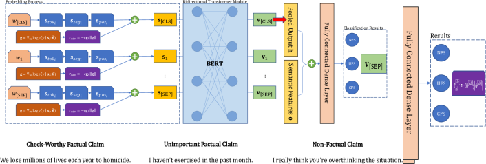
Figure 2. Our Custom Adversarially Perturbed Claim Spotting Architecture

3. BERT Claim Spotting Model

In this section, we present our approach to integrating adversarial training into the BERT architecture for the claim spotting task. To the best of our knowledge, our work is the first to apply gradient-sign adversarial training (Goodfellow et al., 2014) to transformer networks.

3.1. Preliminaries

3.1.1. Task Definition

Detecting check-worthy factual claims has been studied as a binary/ternary classification task and a ranking task, as explained below. In this paper, we evaluate the performance of our models on the binary and ranking task definitions.

Binary Classification Task: In this work a sentence $\mathbf{w}$ is classified as one of two classes, which deviates from the previous definition used in (Hassan et al., 2017b; Jimenez and Li, 2018; Hassan et al., 2017a, 2015).

• Non-Check-Worthy Sentence (NCS): This class includes sentences that contain subjective or opinion-centered statements, questions, and trivial factual claims (e.g., The sky is blue).

• Check-Worthy Factual Sentence (CFS): This class contains claims that are both factual and salient to the general public. They may touch on statistics or historical information, among other things.

Ranking Task: To capture the importance of prioritizing the most check-worthy claims, a check-worthiness score (Hassan et al., 2017a) is defined for each sentence $\mathbf{w}$:

(1) $$CWS=p(y=\text{CFS}\mid\mathbf{w})$$

The $CWS$ score defines a classification model’s predicted probability that a given claim is in the CFS class.

3.1.2. BERT Language Model

Bidirectional Encoder Representations from Transformers (BERT) (Devlin et al., 2019) is a transformer-based language modeling architecture that has recently achieved state-of-the-art performance on many language modeling and text classification tasks, including the Stanford Question Answering Dataset (SQuAD) (Rajpurkar et al., 2016) and General Language Understanding Evaluation (GLUE) (Wang et al., 2018). We review BERT’s relevant features below.

Input/Output Representations: Consider an arbitrary training sentence $\mathbf{w}$ with ground-truth label $y$. $\mathbf{w}$ is first tokenized using the WordPiece Tokenizer (Wu et al., 2016). Next, a [CLS] token is prepended to $\mathbf{w}$ to indicate the start of the sentence, a [SEP] token is appended to $\mathbf{w}$ to indicate the end of a sentence, and $\mathbf{w}$ is padded to a length of $T=200$ using whitespace. Each resulting token is then converted into its corresponding index in the WordPiece vocabulary list. This input vector, denoted $\mathbf{x}\in\mathbb{R}^{T}$, is passed to the embedding layers.

Three-Part Embeddings: $\mathbf{x}$ is first transformed from a sparse bag-of-words form to a dense vector representation (Mikolov et al., 2013) through an embedding lookup matrix $\mathbf{V}\in\mathbb{R}^{Q\times H}$, where $Q$ is the size of the WordPiece vocabulary list and $H$ is the embedding dimensionality. The series of operations that applies $\mathbf{V}$ to $\mathbf{x}$ is called the token embedding layer, and its output is given as $\mathbf{s}_{tok}=\mathbf{V}_{x_{t}},\,\forall x_{t}\in\mathbf{x}$, where $\mathbf{s}_{tok}\in\mathbb{R}^{T\times H}$. Additionally, BERT utilizes an segment embedding layer that signifies which parts of the input contain the input sentence, as the end of $\mathbf{x}$ may be padded with empty space. The output of this layer is denoted by $\mathbf{s}_{seg}\in\mathbb{R}^{T\times H}$. Finally, since vanilla transformers analyze all tokens in parallel and therefore cannot account for the sequential ordering of words, BERT introduces a randomly-initialized real-valued signal via the positional embedding layer to encode the relative order of words. The output of this layer is denoted $\mathbf{s}_{pos}\in\mathbb{R}^{T\times H}$. The final input, denoted $\mathbf{s}$, is the element-wise addition of the three separate embedding layers’ outputs: $\mathbf{s}=\mathbf{s}_{tok}+\mathbf{s}_{seg}+\mathbf{s}_{pos}$. We denote the vector representation of the $t$th token in $\mathbf{x}$ to be $\mathbf{s}_{t}\in\mathbb{R}^{H}$.

Transformer Encoder: Using multiple stacked layers of attention heads (Vaswani et al., 2017), the BERT module encodes each input embedding $\mathbf{s}_{t}$ into a hidden vector $\mathbf{v}_{t}\in\mathbb{R}^{H}$, which is a hidden representation that incorporates context from surrounding words bidirectionally, as opposed to unidirectional encoders used in OpenAI GPT (Radford et al., 2018, 2019).

Pooling Layer: The pooling layer generates a representation for the entire sentence by applying a dense layer on top of the [CLS] token’s hidden representation, resulting in $\mathbf{h}\in\mathbb{R}^{H}$. This sentence-level encoding vector can be used to perform many downstream tasks including claim-spotting.

3.2. Model Architecture

In this section, we outline how BERT is integrated with adversarial perturbations to create a claim-spotting model. The resultant model is end-to-end differentiable and trainable by gradient descent (Kingma and Ba, 2015). We refer the reader to Figure 2 for illustrations on each of the architectural components.

3.2.1. Embedding Process

All three embeddings from the BERT architecture are carried over: token $\mathbf{s}_{pos}$, segment $\mathbf{s}_{seg}$, and positional $\mathbf{s}_{pos}$. Each embedding layer still performs its original function, transforming a given word $\mathbf{x}$ into the embedding representation $\mathbf{s}$. The key difference in our architecture is the implantation of an addition gate through which adversarial perturbations $\mathbf{r}_{adv}$ are injected into $\mathbf{s}$ to create the perturbed embedding $\mathbf{s}^{\prime}$.

3.2.2. BERT Transformer

Our work harnesses the power of the BERT architecture which supports transfer learning (Tan et al., 2018; Radford et al., 2018; Peters et al., 2018; Howard and Ruder, 2018), a process in which weights are loaded from a BERT language model that was pre-trained on billions of English tokens. Denote the number of transformer encoder layers as $L$, the hidden size as $H$, and the number of self-attention heads as $A$. The version of BERT used is $\mathrm{{BERT}_{Base}}$ ($L=12$, $A=12$, $H=768$), which has approximately 110-million parameters. Pretrained model weights for BERT can be found on Google Research’s BERT Repository. 

3.2.3. Fully-Connected Dense Layer

The dense layer is tasked with considering the information passed by BERT’s hidden outputs and determining a classification. To accomplish this, it is implemented as a fully-connected neural network layer that accepts input $\mathbf{h}$ and returns $|\mathbf{k}|$ un-normalized activations in $\mathbf{z}\in\mathbb{R}^{|\mathbf{k}|}$, where $\mathbf{k}=\{0,1\}$, $\mathbf{z}$ is passed through the softmax normalization function to produce final output vector $\hat{\mathbf{y}}$ as:

(2) $$\hat{\mathbf{y}}=\frac{e^{z_{i}}}{\sum_{j\in\mathbf{k}}e^{z_{j}}},\forall i\in\mathbf{k}$$

where each output activation in $\hat{\mathbf{y}}$ represents a classification class. $\hat{\mathbf{y}}$ will later be used to compute the check-worthiness score $CWS$ (Equation 1) and compute the predicted classification label as $\hat{y}=\mathrm{argmax}\,\hat{\mathbf{y}}$.

3.3. Standard Optimization Objective Function

In neural networks, an objective function, also known as the cost or loss function, is a differentiable expression that serves two purposes: to 1) quantify the disparity between the predicted and ground-truth probability distributions and 2) provide a function for gradient descent to minimize. Negative log-likelihood is a highly common choice for the cost function, because it has a nicely computable derivative for optimization via backpropagation, among other advantageous properties (Janocha and Czarnecki, 2017). Our standard negative log-likelihood loss function is formulated as the probability that the model predicts ground-truth $y$ given embedded inputs $\mathbf{s}$, parameterized by the model’s weights $\boldsymbol{\theta}$:

(3) $$\mathcal{L}_{reg}=-\frac{1}{N}\sum_{n=1}^{N}\log p(y^{(n)}\mid\mathbf{s}^{(n)};\boldsymbol{\theta})$$

where $N$ is the total number of training examples in a dataset. $\mathcal{L}_{reg}$ is used to compute adversarial perturbations in Section 3.4.

3.4. Computing Adversarial Perturbations

Gradient-based adversarial training is a regularization technique first introduced in (Goodfellow et al., 2014). The procedure trains classifiers to be resistant to small perturbations to its inputs. Rather than passing regular embedded input $\mathbf{s}$ into a processing module such as a transformer or LSTM, adversarial training passes $\mathbf{s}^{\prime}=\mathbf{s}+\mathbf{r}_{adv}$. $\mathbf{r}_{adv}$ is typically a norm-constrained vector that modifies the input slightly to force the classifier to output incorrect predictions. Then, the disparity between the ground-truth ($y$) and perturbed prediction ($\hat{y}^{\prime}$) based on the perturbed input is minimized through backpropagation, hence training the model to be resistant to these adversarial perturbations. We are particularly interested in adversarial training’s potential as a regularization technique (Shafahi et al., 2019; Dalvi et al., 2004; Nguyen et al., 2015; Shaham et al., 2018; Goodfellow et al., 2014; Miyato et al., 2016), as BERT networks are prone to overfitting when being fine-tuned on small datasets (Sun et al., 2019). To the best of our knowledge, we contribute the first implementation of this technique on transformer networks.

We denote $\boldsymbol{\theta}$ as the parameterization of our neural network and $\mathbf{r}_{adv}$ as a vector perturbation that is added element-wise to $\mathbf{s}$ before being passed to the transformer encoder. $\mathbf{r}_{adv}$ can be computed in several ways. Firstly, random noise may be added to disrupt the classifier. This is typically formalized as sampling $\mathbf{r}_{adv}$ from a Gaussian distribution: $\mathbf{r}_{adv}\sim\mathcal{N}(\mu,\sigma^{2})$. Alternatively, we can compute perturbations that are adversarial, meaning that they increase the model’s negative-log-likelihood error (Equation 3) by the theoretical maximum margin. This achieves the desired effect of generating a perturbation in the direction in which the model is most sensitive. In this case, $\mathbf{r}_{adv}$ is given as:

(4) $$\mathbf{r}_{adv}=\operatornamewithlimits{argmax}\limits_{\mathbf{r},\left\|\mathbf{r}\right\|\leq\epsilon}\>{-\log p(y\mid\mathbf{s}+\mathbf{r};\boldsymbol{\theta})}$$

where $\epsilon$ is a constraint on the perturbation that limits the magnitude of the perturbation.

In (Miyato et al., 2016), it was shown that random noise is a far weaker regularizer than adversarially-computed perturbations. Therefore, we adopt adversarial perturbations for our model (Equation 4) and propose to apply them on the embeddings of the BERT model.

Equation 4 gives the absolute worst-case adversarial perturbation $\mathbf{r}_{adv}$ given a constraint that $\|\mathbf{r}\|\leq\epsilon$. However, this value is impossible to compute with a closed-form analytic solution in neural networks; functions such as Equation 3 are neither convex nor concave in topology. Therefore, we propose a novel technique for generating approximately worst-case perturbations to the model.

Because BERT embeddings are composed of multiple components (Section 3.1.2), it may not be optimal from a regularization standpoint to compute perturbations w.r.t. $\mathbf{s}$. Therefore, to determine the optimal perturbation setting, we propose to experiment with computing $\mathbf{r}_{adv}$ w.r.t. all possible combinations of the 3 embedding components. There are 7 different possible configurations in the set of perturbable combinations $\mathcal{P}$, letting $\mathcal{S}$ denote the set of embedding layers:

(5) $$\mathcal{P}=2^{\mathcal{S}}-\emptyset\text{ where }\mathcal{S}=\{\mathbf{s}_{tok},\mathbf{s}_{seg},\mathbf{s}_{pos}\}$$

Given this list of components that can be perturbed, we denote sum of the subset of the embeddings we will perturb as $\mathbf{m}=\sum_{x\in\mathbf{b}}x$ where $\mathbf{b}\in\mathcal{P}$. We then generate approximate worst-case perturbations by linearizing $\log p(y\mid\mathbf{s};\boldsymbol{\theta})$ with respect to $\mathbf{m}$. To understand what this means, consider the simplified example shown in Figure 3, which graphs an example cost function $J=-\log p(y\mid\mathbf{s};\boldsymbol{\theta})$ with respect to an example embedding space $\mathbf{s}$. For ease of visualization, in Figure 3 it is assumed that $\mathbf{s}$ exists on a scalar embedding space; but in reality, our embeddings are in high-dimensional vector space. The gradient at the point $\mathbf{p}$ gives us information regarding which direction $\mathbf{s}$ should be moved to increase the value of $J$:

(6) $$\Delta\mathbf{s}\propto\frac{\partial}{\partial\mathbf{m}}\log p(y\mid\mathbf{s};\boldsymbol{\theta})$$

However, we must be careful in determining how much $\mathbf{s}$ should be perturbed, because the assumption that $J$ is linear may not hold in reality. If the perturbation is too large, as with $\mathbf{r}_{2}$, the adversarial effect will not be achieved, as the value of $J$ will in fact decrease. However, if we introduce a norm constraint $\epsilon$ to limit the perturbations to a reasonable size, linearization can accomplish the task of approximating a worst-case perturbation, as shown with $\mathbf{r}_{1}$.

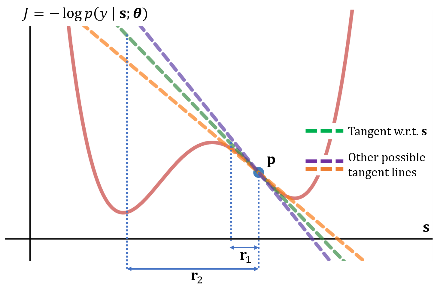
Figure 3. Visualization of Linearization

Given the above insight, we generalize the one-dimensional example (Equation 6) to higher dimensions using the gradient vector. Therefore, the adversarial perturbation $\mathbf{r}_{adv}$ is computed with Equation 7, which can be implemented using backpropagation in deep neural networks:

(7) $$\mathbf{r}_{adv}=-\epsilon\boldsymbol{\omega}/\left\|\boldsymbol{\omega}\right\|_{2}\text{ where }\boldsymbol{\omega}=\nabla_{\mathbf{m}}-\log p(y\mid\mathbf{s};\boldsymbol{\theta})$$

Since we desire to train our language classification model to become resistant to the perturbations defined in Equation 7, we create adversarially-perturbed input embeddings $\mathbf{s}^{\prime}$ as follows:

(8) $$\mathbf{s}^{\prime}=\mathbf{s}+\mathbf{r}_{adv}=\mathbf{s}_{tok}+\mathbf{s}_{seg}+\mathbf{s}_{pos}+\mathbf{r}_{adv}$$

After $\mathbf{s}^{\prime}$ is passed into the transformer module, predictions will be generated. These predictions will be used in formulating the adversarial optimization objective function (Section 3.5).

3.5. Compound Optimization Objective

Our model’s final optimization objective contains two components: standard loss and adversarial loss. Standard loss was defined in Equation 3. Adversarial loss optimizes for distributional smoothness, given by the negative log-likelihood of a model parameterized by $\boldsymbol{\theta}$ predicting $y$ given perturbed input $\mathbf{s}^{\prime}$:

(9) $$\mathcal{L}_{adv}=-\frac{1}{N}\sum_{n=1}^{N}\log p(y^{(n)}\mid\mathbf{s}^{(n)^{\prime}};\boldsymbol{\theta})$$

where $N$ represents the number of training samples in $\mathcal{D}$.

The final optimization objective is given as the sum of $\mathcal{L}_{reg}$ and $\mathcal{L}_{adv}$. By combining the two losses, gradient descent will optimize for both distributional smoothness and model accuracy jointly:

(10) $$\operatornamewithlimits{min}\limits_{\boldsymbol{\theta}}\bigg{\{}\mathcal{L}_{reg}+\lambda\mathcal{L}_{adv}\bigg{\}}$$

where $\lambda$ is a balancing factor between standard and adversarial loss.

3.6. Adversarial Training Algorithm

Let $\boldsymbol{\theta}_{tok}$ be the parameters of the token embedding lookup table, $\boldsymbol{\theta}_{seg}$ be the parameters of the segment embedding layer, and $\boldsymbol{\theta}_{pos}$ be the parameters of the positional embedding layer, $\boldsymbol{\theta}_{n},\forall n<L$ be the parameters for each of the $L$ transformer encoder layers, $\boldsymbol{\theta}_{pool}$ be the parameterization of the pooling layer, and $\boldsymbol{\theta}_{fc}$ be the weights and biases in the fully-connected dense layer. We also define $F$ as the number of encoder layers to freeze (i.e. render the weights uneditable during backpropagation to preserve knowledge obtained from pre-trained weights), where $0\leq F\leq L$.

Input : Training data $\mathcal{D}$

Initialize $\boldsymbol{\theta}_{fc}$ using Xavier method (Glorot and Bengio, 2010);

Load pretrained weights for $\boldsymbol{\theta}_{tok}$, $\boldsymbol{\theta}_{seg}$, $\boldsymbol{\theta}_{pos}$, $\boldsymbol{\theta}_{n},\forall n<L$;

Set $\boldsymbol{\theta}_{tok}$, $\boldsymbol{\theta}_{seg}$, $\boldsymbol{\theta}_{pos}$, and $\boldsymbol{\theta}_{n},\forall n<F$ to untrainable;

$\mathcal{M}\leftarrow$ claim-spotting model (Figure 2);

while not converge do

       Sample $\mathbf{w}$, $y$ from data $\mathcal{D}$;

       Tokenize and process $\mathbf{w}$ into $\mathbf{x}$;

       Pass $\mathbf{x}$ through embeddings to produce $\mathbf{s}$;

      

      $\triangleright$ Standard forward-propagation

       $\hat{y}\leftarrow\mathcal{M}(\mathbf{s};\,\boldsymbol{\theta})$;

       Compute $\mathcal{L}_{reg}$ using $y,\hat{y}$ (Equation 3);

      

      $\triangleright$ Generate and apply perturbations

       Compute $\mathbf{r}_{adv}$ using $\mathcal{L}_{reg},y$ (Equation 7);

       Compute perturbed input as $\mathbf{s}^{\prime}=\mathbf{s}+\mathbf{r}_{adv}$;

      

      $\triangleright$ Adversarial forward-propagation

       $\hat{y}^{\prime}\leftarrow\mathcal{M}(\mathbf{s}^{\prime};\,\boldsymbol{\theta})$;

       Compute $\mathcal{L}_{adv}$ using $y,\hat{y}^{\prime}$ (Equation 9);

      

      $\triangleright$ Adversarial training

       Optimize $\left\{\mathcal{L}_{reg}+\lambda\mathcal{L}_{adv}\right\}$ (Equation 10);

      

end while

Algorithm 1 Adversarial Training Loop

The adversarial training procedure is shown in Algorithm 1. First, model $\mathcal{M}$ is used to compute the optimization function $\mathcal{L}_{reg}$. Then, $\mathcal{L}_{reg}$ is used to compute the adversarial perturbation (Equation 7), which is used to compute the adversarial optimization objective (Equation 9). This objective is added to the standard objective (Equation 10) and minimized using gradient descent.

4. Results and Discussions

Table 1. Sample Sentences, Labels, and Check-Worthiness Scores

Claim	Label	CB-SVM CWS Score	CB-BBA CWS Score
The U.S. loses millions of lives each year to homicide.	CFS	0.6000	0.9999
I really think you’re overthinking the situation.	NCS	0.2178	$5.8515\text{\times}{10}^{-05}$

We evaluate our new transformer-based claim-spotting models on both the Classification and Ranking Tasks (Section 3.1.1). We compare against re-trained and refined versions of past ClaimBuster models (Hassan et al., 2017a; Jimenez and Li, 2018) and the top-two performing systems from the 2019 CLEF-CheckThat! Challenge. Table 1 shows several example sentences, their ground-truth labels, and our models’ $CWS$ scores.

4.1. Experiment Setup

4.1.1. Datasets

We use two claim-spotting datasets to evaluate model performance.

ClaimBuster Dataset (CBD): The ClaimBuster dataset is our own in-house, manually labeled dataset. A different version of the CBD was used by (Hassan et al., 2017a; Hassan et al., 2017b; Jimenez and Li, 2018). The current CBD consists of two classes, as mentioned in Section 3.1.1: NCS and CFS. The switch to this scheme was motivated by our observation that the non-check-worthy factual sentence class in the previous versions of CBD was not really useful and possibly negatively impacting models trained using it. The CBD consists of 9674 sentences (6910 NCS and 2764 CFS). For validation we perform 4-fold cross validation using this same dataset. The dataset is composed of manually labeled sentences from all U.S. presidential debates from 1960 to 2016. We describe the details of dataset collection in Section 7.3.2. This dataset is publicly available, as noted in Section 7.3.

CLEF2019-CheckThat! Dataset (C₂₀₁₉): We also evaluate our model on the 2019 CLEF-CheckThat!  claim-spotting dataset. CLEF-CheckThat! is an annual competition that assesses the state-of-the-art in automated computational fact-checking by providing datasets for claim-spotting. The C₂₀₁₉ dataset is comprised of political debate and interview transcripts. Sentences are labelled as check-worthy only if they were fact-checked by FactCheck.org. Note that this labelling strategy introduces significant bias into the dataset, as many problematic claims go unchecked due to the limited resources of fact-checkers from a single organization (Section 1). The training set contains 15,981 non-check-worthy and 440 check-worthy sentences, and the testing set contains 6,943 non-check-worthy and 136 check-worthy sentences. The C₂₀₁₉ dataset also includes speaker information for each sentence, which we did not use in training our models for two reasons: (1) it may introduce unwanted bias based on the name (or guid if names are masked) of speaker and (2) it makes the claim spotting model inapplicable to real-time events since live transcripts typically lack speaker information and speakers not present in the training set are likely to be encountered as well.

4.2. Evaluated Models

CB-BBA: This model is trained using our novel claim-spotting framework detailed in Section 3.2. It is trained adversarially using the compound optimization objective defined in Equation 10.

CB-BB: This model is architecturally identical to CB-BBA but is trained using the standard optimization objective (Equation 3). In implementation, $\mathbf{r}_{adv}$ is simply set to $0$. This model serves as a point of comparison for the adversarial model.

CB-BiL: (Jimenez and Li, 2018) This model is a reimplementation of (Jimenez and Li, 2018) in TensorFlow 2.1. It uses normalized GloVe word embeddings  and consists of a bi-directional LSTM layer which allows it to capture forward and reverse sequence relationships. The model’s binary cross entropy loss function is optimized using RMSProp.

CB-SVM: (Hassan et al., 2015, 2017a) The SVM classifier uses a linear kernel. The feature-vector used to represent each sentence is composed of a tf-idf weighted bag-of-unigrams vector, part-of-speech vector, and sentence length (i.e., number of words). The total number of features for each sentence using our dataset is $6980$. The core SVM model is produced using scikit-learn’s LinearSVC class with the max number of iterations set to an arbitrary high number ($10000000$), to ensure model convergence.

4.2.1. 2019 CLEF-CheckThat! Models

Neither of the top two teams in CLEF2019 released their code; therefore, we are only able to retrieve their results on CLEF2019.

Copenhagen (Hansen et al., 2019): Team Copenhagen’s model, the top performer on C₂₀₁₉, consisted of an LSTM model (Hochreiter and Schmidhuber, 1997) token embeddings fused with syntactic-dependency embeddings. To train their model, Copenhagen did not use the C₂₀₁₉ dataset, instead using an external dataset of Clinton/Trump debates that was weakly labeled using our ClaimBuster API. footnote 14

TheEarthIsFlat (Favano et al., 2019): TheEarthIsFlat, the second-place performer, used a feed-forward neural network trained on the C₂₀₁₉ dataset. They encoded sentences using the Universal Sentence Encoder (Cer et al., 2018).

4.3. Embedding Perturbation Study Results

Table 2. Perturbation Combinations Study Results
Averaged Across Stratified 4-Fold Cross Validation

	P		R		F1
ID	NCS	CFS	NCS	CFS	NCS	CFS
0	0.9225	0.8585	0.9472	0.8010	0.9347	0.8287
1	0.9227	0.8453	0.9412	0.8028	0.9319	0.8235
2	0.9330	0.8382	0.9357	0.8321	0.9344	0.8351
3	0.9295	0.8424	0.9385	0.8220	0.9340	0.8321
4	0.9201	0.8641	0.9501	0.7938	0.9349	0.8275
5	0.9282	0.8547	0.9444	0.8173	0.9362	0.8356
6	0.9335	0.8445	0.9386	0.8329	0.9361	0.8386
0	1	2	3	4	5	6
pos seg tok	pos seg	pos tok	seg tok	pos	seg	tok

In Table 2, we see the results of perturbing the 3 different embedding layers in BERT. From the results we conclude that setting $6$ produces the best models for our task. Particularly, this setting produces the best recall for the CFS class, which is arguably the more important class. The sacrifice in recall, with respect to the NCS class, compared to other settings is only $\approx 0.02$ at most. While setting $4$ achieves the best performance in precision with respect to the CFS class, the drop in recall for the CFS class makes it not viable. Thus, from here on, any results dealing with adversarial training will employ setting $6$ and perturb only the tok embedding layer.

4.4. Classification Task, Ranking, and Distribution Results

Table 3. Precision, Recall, and F1 Averaged Across Stratified 4-Fold Cross Validation

Model	P		Pm	Pw	R		Rm	Rw	F1		F1m	F1w
	NCS	CFS			NCS	CFS			NCS	CFS
CB-SVM	0.8935	0.7972	0.8454	0.8660	0.9263	0.7240	0.8251	0.8685	0.9096	0.7588	0.8342	0.8665
CB-BiL	0.9067	0.7773	0.8420	0.8697	0.9123	0.7652	0.8387	0.8703	0.9095	0.7712	0.8403	0.8700
CB-BB	0.9344	0.8149	0.8747	0.9003	0.9239	0.8379	0.8809	0.8993	0.9291	0.8263	0.8777	0.8997
CB-BBA	0.9335	0.8445	0.8890	0.9081	0.9386	0.8329	0.8857	0.9084	0.9361	0.8386	0.8873	0.9082

Table 4. nDCG Averaged Across
Stratified 4-Fold Cross Validation

	CB-SVM	CB-BiL	CB-BB	CB-BBA
nDCG	0.9765	0.9817	0.9877	0.9894

4.4.1. Classification Results

Our results are encapsulated in Table 3 and Table 4. We assume familiarity with the metrics, which are defined in Section 7.2. In Table 3, we observe that the SVM based model, CB-SVM, has the lowest performance across many measures. This is expected, as the SVM can only capture the information present in the dataset, while the deep learning models benefit from outside knowledge afforded to them by either pre-trained word-embeddings or a pre-trained model (i.e., BERT) that can be fine tuned. The CB-BiL model shows modest improvements overall, but it does achieve noticeably better CFS recall than the SVM model. With respect to BERT-based architectures, both models outperform CB-SVM and CB-BiL considerably. Between CB-BB and CB-BBA, CB-BBA achieves the best performance across most of the metrics. Although CB-BB has a better CFS recall and NFS precision, these differences are minuscule and not enough for CB-BB to be considered a better model. Ultimately, CB-BBA achieves a 4.70 point F1 score improvement over the past state-of-the-art CB-BiL model, a 5.31 point F1-score improvement over the CB-SVM model, and a 0.96 point F1-score improvement over a regularly-trained BERT model. This demonstrates the effectiveness of our new architecture and training algorithm.

The results on the C₂₀₁₉ dataset are in Table 5. The metrics presented for the CLEF competition teams are taken from (Atanasova et al., 2019), since we could not find the source code to reproduce them. For this reason we also cannot provide the P, R, F1, and nDCG for these teams. We tested models trained on both the CBD and C₂₀₁₉ training set and used the C₂₀₁₉ testing set to evaluate them. The models trained on CBD and tested on the CLEF test set didn’t perform as well; this was expected, given that our methodology of dataset labelling differs significantly from CLEF’s. Despite this, when trained on C₂₀₁₉, CB-BBA held its own when compared to the Copenhagen model which was the winner of that competition only falling short in the mAP metric by 0.0035.

4.4.2. nDCG Results

In Table 4 we observe that the best nDCG score is achieved by the CB-BBA model, and the CB-BB and CB-BiL models are within $\approx\frac{6}{1000}$ of it. The CB-SVM model has the “worst” nDCG, but is still not far behind the deep learning models. It is noteworthy that all models show relatively good performance on this measure since the CFS class is less represented in the dataset.

4.4.3. Distribution of $CWS$ Scores

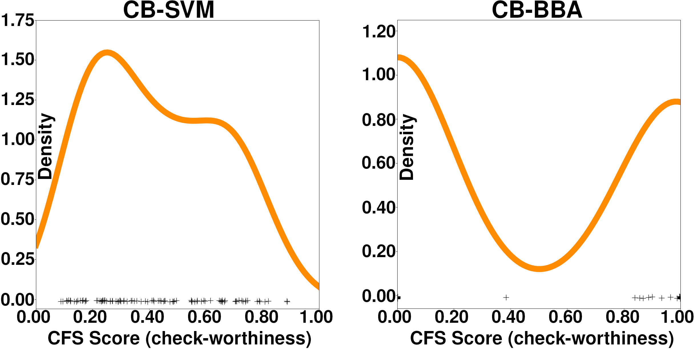
Figure 4. Comparison of Check-Worthiness Score Distributions Using the CB-BBA and CB-SVM Models on 100 sentences from the January 14^th, 2020, Democratic presidential debate.

To analyze the distribution of our models’ outputs on a typical corpus of text, we process 100 sentences from the January 14^th, 2020 Democratic presidential debate.  The sentences were chosen so that there would be about equal numbers of check-worthy and non-check-worthy sentences. Figure 4 displays the results, which use Kernel Density Estimation (Rosenblatt, 1956) to estimate the score distribution from discrete data points. Observing the density spikes around 0 and 1 on CB-BBA’s distribution, we conclude that our model more clearly differentiates sentences as check-worthy or not check-worthy. The more well-delineated distribution of the CB-BBA model also improves its interpretability over CB-SVM.

Table 5. CLEF-2019 Test Dataset Classification and Ranking Task Results

Model	Training Dataset	mAP	P@10	P@20	P@50	P		R		F1		nDCG
						NCS	CFS	NCS	CFS	NCS	CFS
Copenhagen	C2019	0.1660	0.2286	0.1571	0.1143
TheEarthIsFlat	C2019	0.1597	0.2143	0.1857	0.1457
CB-SVM	C2019	0.1087	0.1429	0.1429	0.1114	0.9813	0.2105	0.9978	0.0294	0.9895	0.0516	0.4567
CB-BBA	C2019	0.1625	0.2571	0.1929	0.1086	0.9812	0.5000	0.9996	0.0221	0.9903	0.0423	0.5181
CB-SVM	CBD	0.1134	0.1571	0.1429	0.1143	0.9885	0.0678	0.8694	0.4853	0.9251	0.1190	0.4744
CB-BBA	CBD	0.1363	0.1286	0.1286	0.1229	0.9926	0.0752	0.8354	0.6838	0.9073	0.1356	0.4978

5. Related Works

In recent years, there have been several efforts with respect to building claim spotting models. ClaimBuster (Hassan et al., 2015) is the first of several notable claim spotting models. Another team (Gencheva et al., 2017) extended CB-SVM feature set 4.2 by including several contextual features such as: position of the target sentence in its segment, speaker name, interaction between opponents, etc. They created a dataset from the 2016 US presidential and vice presidential debates and annotated sentences by taking fact-checking outputs from 9 fact-checking organizations. If a sentence was fact-checked by at least one fact-checking outlet, it was labeled as check-worthy. A follow-up study (Jaradat et al., 2018) built an online system, namely, ClaimRank footnote 15 for prioritizing sentences for fact-checking based on their check-worthiness score. ClaimRank is a re-implementation of the aforementioned study, but it also supports Arabic by employing cross-language English-Arabic embeddings. Another study (Patwari et al., 2017) followed the same data annotation strategy on a larger dataset by including sentences from an additional 15 2016 U.S. primary debates. The authors developed a multi-classifier based model called TATHYA that uses multiple SVMs trained on different clusters of the dataset. The model takes the output from the most confident classifier. The feature set used was comprised of tf-idf weighted bag-of-unigrams, topics of the sentences, part-of-speech tuples, and a count of entities.

Another effort by Konstantinovskiy et al. (Konstantinovskiy et al., 2018), which utilized the expertise of professional fact-checkers, designed an annotation schema and created a benchmark dataset for training a claim spotting model. The authors trained the model using logistic regression on top of dataset’s universal sentence representation derived from InferSent (Conneau et al., 2017). Their model classifies a sentence as either checkable or non-checkable. The authors also disagreed with ClaimBuster’s and ClaimRank’s idea of a check-worthiness score. They believe the decision of how important a claim is, should be left to the professional fact-checkers. In the recent CLEF2019 competition on check-worthiness detection, the Copenhagen team developed the winning approach (Hansen et al., 2019) which leveraged the semantic and syntactic representation of each word in a sentence. They generated domain-specific pretrained word embeddings that helped their system achieve better performance in the competition. They used a large weakly-labeled dataset, whose labels were assigned by ClaimBuster, for training an LSTM model.

6. Conclusion

We have presented our work on detecting check-worthy factual claims employing adversarial training on transformer networks. Our results have shown that through our methods we have achieved state-of-the-art results on two different datasets (i.e., CBD and C₂₀₁₉). During the process we also re-vamped our dataset and approach to collecting and assigning labels for it. We have also come to realize that the lack of a large standardized dataset holds this field back, and thus we look forward to contributing and establishing efforts to fix this situation. We plan on releasing different versions of our dataset periodically in hopes that we can get more significant community contributions with respect to expanding it. 

In the future, we are interested in exploring adversarial training as a defense against malicious adversaries. As a publicly deployed API, ClaimBuster may be susceptible to exploitation without incorporating mechanisms that improve its robustness. For example, it has been shown by (Jin et al., 2019) that a model’s classification can be strongly influenced when certain words are replaced by their synonyms. We are currently researching methods to combat similar weaknesses.

7. Reproducibility

7.1. Code Repositories, API, and Related Projects

We provide an API of the claim-spotting algorithm online to show its real-world usage at https://idir.uta.edu/claimbuster/api/docs/. We are also releasing our code along with detailed instructions on running and training our models. Our code and its documentation can be found at https://github.com/idirlab/claimspotter. Along with these, we also present several projects which showcase how ClaimBuster can and is currently being used:

• Claimspotting Presidential Debates 

• End-to-End Fact-Checking 

• Claimspotting Tweets 

7.2. Formulas for Performance Measures

Precision (P):

(11) $$\mathrm{P}=\frac{TP}{TP+FP}$$

Recall (R):

(12) $$\mathrm{R}=\frac{TP}{TP+FN}$$

F1:

(13) $$\mathrm{F1}=2\times\frac{P\times R}{P+R}$$

$\mathbf{\left\{P,R,F1\right\}}$ Macro (P_m, R_m, F1_m):

(14) $$\begin{gathered}\mathrm{M}_{m}=\frac{1}{|\mathbf{L}|}\sum_{l\in\mathbf{L}}M_{l}\\ \textrm{where }M\in\left\{P,R,F1\right\}\textrm{, and }L\in\left\{NCS,CFS\right\}\end{gathered}$$

$\mathbf{\left\{P,R,F1\right\}}$ Weighted (P_w, R_w, F1_w):

(15) $$\begin{gathered}\mathrm{M}_{w}=\frac{1}{{\sum_{l\in\mathbf{L}}N_{l}}}\sum_{l\in\mathbf{L}}N_{l}\times M_{l}\\ \textrm{where }M\in\left\{P,R,F1\right\}\textrm{, }L\in\left\{NCS,CFS\right\}\textrm{, and}\\ N_{l}\textrm{ is the number of samples whose ground truth label is $l$.}\end{gathered}$$

Mean Average Precision (MAP):

(16) $$\begin{gathered}AP=\frac{\sum_{k=1}^{n}\left(P\left(k\right)\times rel\left(k\right)\right)}{\textit{number of check-worthy claims}}\\ \textrm{where }P\left(k\right)\textrm{ is the precision at k, and }rel\left(k\right)\textrm{ equals 1 if the}\\ \textrm{claim is check-worthy and 0 otherwise.}\\ MAP=\frac{\sum_{q}^{Q}AP\left(q\right)}{Q}\\ \textrm{where }Q\textrm{ is the number of queries.}\end{gathered}$$

Normalized Discounted Cumulative Gain (nDCG):

(17) $$\begin{gathered}nDCG_{p}=\frac{\sum_{i=1}^{p}\frac{2^{rel_{i}}-1}{log_{2}\left(i+1\right)}}{\sum_{i=1}^{\left|REL_{p}\right|}\frac{2^{rel_{i}}-1}{log_{2}\left(i+1\right)}}\\ \textrm{where }rel_{i}\in\left\{0,1\right\}\textrm{is the {CWS} at position }i\textrm{, and }\\ \left|REL_{p}\right|\textrm{represents the list of claims ordered by their}\\ \textrm{check-worthiness up to position }p\textrm{.}\end{gathered}$$

7.3. Datasets

We provide the CBD dataset, a collection of sentences labelled manually in-house by high-quality coders, in our repository at https://github.com/idirlab/claimspotter/tree/master/data. CBD was curated to have $N_{NCS}=Y\times N_{CFS}$, for $Y=2.5$; where $N_{NCS}$ is the number of non-check-worthy sentences and $N_{CFS}$ is the number of check-worthy sentences. This was done after evaluating different values of $Y$ (i.e., $Y\in\{2,2.5,3\}$) and concluding the best ratio for NCS to CFS was $2.5:1$. The C₂₀₁₉ dataset, containing sentences from the first and second presidential debates and the first vice presidential debate from 2016, can be found at https://github.com/clef2018-factchecking/clef2018-factchecking.

7.3.1. Contributing

We are always looking for collaborators to contribute to the labelling of more data. Contributions will benefit everyone as we plan on releasing periodic updates when a significant amount of new labels are gathered. To contribute please visit and make an account at: https://idir.uta.edu/classifyfact_survey/.

7.3.2. Dataset Labeling Criteria

The labels for the dataset are assigned by high-quality coders, which are participants that have a pay-rate $\geq 5\textrm{\cent}$ and have labeled at least $100$ sentences. The pay-rate for a user is internally calculated by taking into account their labeling quality, the average length of sentence a user labels, and how many sentences a user skips. More specifically, we define the quality ($LQ_{p}$) of a coder ($p$) with respect to the screening sentences they have labeled ($SS(p)$) as:

$$LQ_{p}=\frac{\sum_{s\in SS(p)}\gamma^{lt}}{|SS(p)|}$$

where $\gamma^{lt}$ is the weight factor when $p$ labeled the screening sentence $s$ as $l$ and the experts labeled it as $t$. Both $l,t\in\{NCS$, $CFS\}$. We set $\gamma^{lt}=-0.2$ where $l=t$, $\gamma^{lt}=2.5$ where $(l,t)\in\{(NCS,CFS),(CFS,NCS)\}$. The weights are set empirically. The pay-rate ($R_{p}$) is then defined as:

$$R_{p}=\frac{L_{p}}{L}^{1.5}\times(3-\frac{7\times LQ_{p}}{0.2})\times 0.6^{\frac{|SKIP_{p}|}{|ANS_{p}|}}$$

where, $L$ is the average length of all the sentences, $L_{p}$ is the average length of sentences labeled by $p$, $ANS_{p}$ is the set of sentences labeled by $p$ and $SKIP_{p}$ is the set of sentences skipped by $p$. The numerical values in the above equation were set in such a way that it would be possible for a participant to earn up to $10\textrm{\cent}$ per sentence. Using this scheme, out of $581$ users in our system, $69$ users are considered high-quality coders. A label is then only assigned to a particular sentence if it has unanimously been assigned that label by at least 2 high-quality coders. More precisely, we defined the number of high-quality labels needed as: $X\in\left[NCS,CFS\right],\exists X\ni s_{X}\geq 2\wedge s_{X}=s_{NCS}+s_{CFS}$ where, $s_{X}$ is the number of top-quality labels of type $X$, and a top quality label is one that has been given by a high-quality coder (Hassan et al., 2017a).

7.4. Hyperparameters

Table 6. Major Parameters for Training

Parameter	BBA	BB
cs_train_steps	10	5
cs_lr	5e-5	5e-5
cs_kp_cls	0.7	0.7
cs_batch_size_reg	24	24
cs_batch_size_adv	12	-
cs_perturb_norm_length	2.0	-
cs_lambda	0.1	-
cs_combine_reg_adv_loss	True	-
cs_perturb_id	5	-

We provide Table 6 for major parameter settings used in the BBA, BB, and BiLSTM claimspotting algorithm. The description of the major parameters are as follows:

• cs_train_steps: number of epochs to run

• cs_lr: learning rate during optimiation

• cs_perturb_norm_length: norm length of adversarial perturbation

• cs_kp_cls: keep probability of dropout in fully connected layer

• cs_lambda: adversarial loss coefficient (eq. 10)

• cs_combine_reg_adv_loss: add loss of regular and adversarial loss during training

• cs_batch_size_reg: size of the batch

• cs_batch_size_adv: size of the batch when adversarial training

• cs_perturb_id: index in Table 2

7.5. Evaluation and Training Final Models

We perform 4-fold cross validation to evaluate our models, selecting the best model from each fold using the weighted F1-score (eq.  15) calculated on the validation set. Therefore, in each iteration the data is split as follows: $25\%$ test, $7.5\%$ validation, and $67.5\%$ training. The metrics produced at the end are based on the classifications across all folds. We train the final models (for both CBD and C₂₀₁₉) on the entire dataset for up to 10 epochs and select the best epoch based on the weighted F1-score calculated on the validation set.

7.6. Hardware and Software Specifications

Our neural network models and training algorithms were written in TensorFlow 2.1 (Abadi et al., 2016) and run on machines with four Nvidia GeForce GTX 1080Ti GPU’s. We did not parallelize GPU usage with distributed training; each experiment was run on a single 1080Ti GPU. The machines ran Arch Linux and had an 8-Core i7 5960X CPU, 128GB RAM, 4TB HDD, and 256GB SSD.

References

- (1)
- Abadi et al. (2016) Martin Abadi, Paul Barham, Jianmin Chen, Zhifeng Chen, et al. 2016. TensorFlow: A system for large-scale machine learning. In OSDI. 265–283.
- Allcott and Gentzkow (2017) Hunt Allcott and Matthew Gentzkow. 2017. Social Media and Fake News in the 2016 Election. Working Paper 23089. National Bureau of Economic Research.
- Atanasova et al. (2019) Pepa Atanasova, Preslav Nakov, Georgi Karadzhov, Mitra Mohtarami, and Giovanni Da San Martino. 2019. Overview of the CLEF-2019 CheckThat! Lab on Automatic Identification and Verification of Claims. Task 1: Check-Worthiness. In CEUR Workshop Proceedings.
- Caruana et al. (2001) Rich Caruana, Steve Lawrence, and C Lee Giles. 2001. Overfitting in neural nets: Backpropagation, conjugate gradient, and early stopping. In NIPS. 402–408.
- Cer et al. (2018) Daniel Cer, Yinfei Yang, Sheng-yi Kong, Nan Hua, Nicole Limtiaco, Rhomni St John, Noah Constant, Mario Guajardo-Cespedes, Steve Yuan, Chris Tar, et al. 2018. Universal sentence encoder. arXiv:1803.11175
- Chan et al. (2017) Man-pui Sally Chan, Christopher R. Jones, Kathleen Hall Jamieson, and Dolores Albarracín. 2017. Debunking: A Meta-Analysis of the Psychological Efficacy of Messages Countering Misinformation. Psychological Science 28, 11 (Sep 2017), 1531–1546.
- Conneau et al. (2017) Alexis Conneau, Douwe Kiela, Holger Schwenk, Loic Barrault, and Antoine Bordes. 2017. Supervised learning of universal sentence representations from natural language inference data. arXiv:1705.02364
- Dalvi et al. (2004) Nilesh Dalvi, Pedro Domingos, Sumit Sanghai, Deepak Verma, et al. 2004. Adversarial classification. In SIGKDD. 99–108.
- Devlin et al. (2019) Jacob Devlin, Ming-Wei Chang, Kenton Lee, and Kristina Toutanova. 2019. BERT: Pre-training of Deep Bidirectional Transformers for Language Understanding. In NAACL. 4171–4186.
- Favano et al. (2019) Luca Favano, Mark J. Carman, and Pier Luca Lanzi. 2019. TheEarthIsFlat’s Submission to CLEF’19 CheckThat! Challenge. In CEUR Workshop Proceedings.
- Gencheva et al. (2017) Pepa Gencheva, Preslav Nakov, Lluís Màrquez, Alberto Barrón-Cedeño, and Ivan Koychev. 2017. A context-aware approach for detecting worth-checking claims in political debates. In RANLP. 267–276.
- Glorot and Bengio (2010) Xavier Glorot and Yoshua Bengio. 2010. Understanding the difficulty of training deep feedforward neural networks. In AISTATS. 249–256.
- Goodfellow et al. (2014) Ian J Goodfellow, Jonathon Shlens, and Christian Szegedy. 2014. Explaining and harnessing adversarial examples. arXiv:1412.6572
- Hansen et al. (2019) Casper Hansen, Christian Hansen, Jakob Grue Simonsen, and Christina Lioma. 2019. Neural Weakly Supervised Fact Check-Worthiness Detection with Contrastive Sampling-Based Ranking Loss. In CEUR Workshop Proceedings.
- Hassan et al. (2017a) Naeemul Hassan, Fatma Arslan, Chengkai Li, and Mark Tremayne. 2017a. Toward Automated Fact-Checking: Detecting Check-worthy Factual Claims by ClaimBuster. In SIGKDD. 1803–1812.
- Hassan et al. (2015) Naeemul Hassan, Chengkai Li, and Mark Tremayne. 2015. Detecting check-worthy factual claims in presidential debates. In CIKM. 1835–1838.
- Hassan et al. (2017b) Naeemul Hassan, Gensheng Zhang, Fatma Arslan, Josue Caraballo, and et al. 2017b. ClaimBuster: The First-ever End-to-end Fact-checking System. PVLDB 10, 12 (Aug. 2017), 1945–1948.
- Heilman (2011) Michael Heilman. 2011. Automatic Factual Question Generation from Text. Ph.D. Dissertation. USA. Advisor(s) Smith, Noah A.
- Hochreiter and Schmidhuber (1997) Sepp Hochreiter and Jürgen Schmidhuber. 1997. Long short-term memory. Neural computation 9, 8 (1997), 1735–1780.
- Howard and Ruder (2018) Jeremy Howard and Sebastian Ruder. 2018. Universal Language Model Fine-tuning for Text Classification. In ACL.
- Janocha and Czarnecki (2017) Katarzyna Janocha and Wojciech Marian Czarnecki. 2017. On Loss Functions for Deep Neural Networks in Classification. Schedae Informaticae 1/2016 (2017).
- Jaradat et al. (2018) Israa Jaradat, Pepa Gencheva, Alberto Barrón-Cedeño, Lluís Màrquez, and Preslav Nakov. 2018. ClaimRank: Detecting Check-Worthy Claims in Arabic and English. In NAACL. 26–30.
- Jimenez and Li (2018) Damian Jimenez and Chengkai Li. 2018. An Empirical Study on Identifying Sentences with Salient Factual Statements. In IJCNN. 1–8.
- Jin et al. (2019) Di Jin, Zhijing Jin, Joey Tianyi Zhou, and Peter Szolovits. 2019. Is bert really robust? natural language attack on text classification and entailment. arXiv preprint arXiv:1907.11932 (2019).
- Kingma and Ba (2015) Diederik P. Kingma and Jimmy Ba. 2015. Adam: A Method for Stochastic Optimization. In ICLR.
- Konstantinovskiy et al. (2018) Lev Konstantinovskiy, Oliver Price, Mevan Babakar, and Arkaitz Zubiaga. 2018. Towards automated factchecking: Developing an annotation schema and benchmark for consistent automated claim detection. arXiv:1809.08193
- Majithia et al. (2019) Sarthak Majithia, Fatma Arslan, Sumeet Lubal, Damian Jimenez, Priyank Arora, Josue Caraballo, and Chengkai Li. 2019. ClaimPortal: Integrated Monitoring, Searching, Checking, and Analytics of Factual Claims on Twitter. In ACL. 153–158.
- Mikolov et al. (2013) Tomas Mikolov, Ilya Sutskever, Kai Chen, Greg S Corrado, and Jeff Dean. 2013. Distributed representations of words and phrases and their compositionality. In NIPS. 3111–3119.
- Miyato et al. (2016) Takeru Miyato, Andrew M Dai, and Ian Goodfellow. 2016. Adversarial training methods for semi-supervised text classification. arXiv:1605.07725
- Miyato et al. (2018) Takeru Miyato, Shin-ichi Maeda, Masanori Koyama, and Shin Ishii. 2018. Virtual adversarial training: a regularization method for supervised and semi-supervised learning. IEEE transactions on pattern analysis and machine intelligence 41, 8 (2018), 1979–1993.
- Nadeem et al. (2019) Moin Nadeem, Wei Fang, Brian Xu, Mitra Mohtarami, and James Glass. 2019. FAKTA: An Automatic End-to-End Fact Checking System. In NAACL.
- Nguyen et al. (2015) Anh Nguyen, Jason Yosinski, and Jeff Clune. 2015. Deep neural networks are easily fooled: High confidence predictions for unrecognizable images. In CVPR.
- Nyhan and Reifler (2015) Brendan Nyhan and Jason Reifler. 2015. Estimating fact-checking‘s effects. (2015). https://www.americanpressinstitute.org/wp-content/uploads/2015/04/Estimating-Fact-Checkings-Effect.pdf
- Patwari et al. (2017) Ayush Patwari, Dan Goldwasser, and Saurabh Bagchi. 2017. TATHYA: A multi-classifier system for detecting check-worthy statements in political debates. In CIKM. 2259–2262.
- Pennycook and Rand (2019) Gordon Pennycook and David G Rand. 2019. Fighting misinformation on social media using crowdsourced judgments of news source quality. Proceedings of the National Academy of Sciences 116, 7 (2019), 2521–2526.
- Peters et al. (2018) Matthew Peters, Mark Neumann, Mohit Iyyer, Matt Gardner, Christopher Clark, Kenton Lee, and Luke Zettlemoyer. 2018. Deep Contextualized Word Representations. In NAACL.
- Radford et al. (2018) Alec Radford, Karthik Narasimhan, Tim Salimans, and Ilya Sutskever. 2018. Improving language understanding by generative pre-training.
- Radford et al. (2019) Alec Radford, Jeffrey Wu, Rewon Child, David Luan, Dario Amodei, and Ilya Sutskever. 2019. Language models are unsupervised multitask learners. OpenAI Blog 1, 8 (2019), 9.
- Rajpurkar et al. (2016) Pranav Rajpurkar, Jian Zhang, Konstantin Lopyrev, and Percy Liang. 2016. SQuAD: 100,000+ Questions for Machine Comprehension of Text. In EMNLP.
- Rosenblatt (1956) Murray Rosenblatt. 1956. Remarks on Some Nonparametric Estimates of a Density Function. The Annals of Mathematical Statistics 27, 3 (09 1956), 832–837.
- Shafahi et al. (2019) Ali Shafahi, Mahyar Najibi, Amin Ghiasi, Zheng Xu, John Dickerson, Christoph Studer, Larry S. Davis, Gavin Taylor, and Tom Goldstein. 2019. Adversarial Training for Free! arXiv:1904.12843
- Shaham et al. (2018) Uri Shaham, Yutaro Yamada, and Sahand Negahban. 2018. Understanding adversarial training: Increasing local stability of supervised models through robust optimization. Neurocomputing 307 (2018), 195–204.
- Sun et al. (2019) Chi Sun, Xipeng Qiu, Yige Xu, and Xuanjing Huang. 2019. How to Fine-Tune BERT for Text Classification? arXiv:1905.05583
- Tan et al. (2018) Chuanqi Tan, Fuchun Sun, Tao Kong, Wenchang Zhang, Chao Yang, and Chunfang Liu. 2018. A Survey on Deep Transfer Learning. Lecture Notes in Computer Science (2018), 270–279.
- Vaswani et al. (2017) Ashish Vaswani, Noam Shazeer, Niki Parmar, Jakob Uszkoreit, Llion Jones, Aidan N. Gomez, Lukasz Kaiser, and Illia Polosukhin. 2017. Attention Is All You Need. arXiv:1706.03762
- Wang et al. (2018) Alex Wang, Amanpreet Singh, Julian Michael, Felix Hill, Omer Levy, and Samuel R Bowman. 2018. Glue: A multi-task benchmark and analysis platform for natural language understanding. arXiv:11804.07461
- Wu et al. (2016) Yonghui Wu, Mike Schuster, Zhifeng Chen, Quoc V. Le, and et al. 2016. Google’s Neural Machine Translation System: Bridging the Gap between Human and Machine Translation. arXiv:1609.08144