Network Theoretic Analysis of Maximum a Posteriori Detectors for Optimal Input Detection111This material is based upon work supported in part by ARO award 71603NSYIP and in part by UCOP award LFR-18-548175.
Abstract
This paper considers maximum-a-posteriori (MAP) and linear discriminant based MAP detectors to detect changes in the mean and covariance of a stochastic input, driving specific network nodes, using noisy measurements from sensors non-collocated with the input nodes. We explicitly characterize both detectors’ performance in terms of the network edge weights and input and sensor nodes’ location. In the asymptotic measurement regime, when the input and measurement noise are jointly Gaussian, we show that the detectors’ performance can be studied using the input to output gain of the system’s transfer function matrix. Using this result, we obtain conditions for which the detection performance associated with the sensors on a given network cut is better (or worse) than that of the sensors associated with the subnetwork induced by the cut and not containing the input nodes. Our results also provide structural insights into the sensor placement from a detection-theoretic viewpoint. We validate our theoretical findings via multiple numerical examples.
keywords:
Statistical hypotheses testing , mean detection , covariance detection , network systems, sensor placement1 Introduction
Security of cyber-physical networks is of timely and utmost importance [1]. In recent years, researchers have proposed a number of model-based and heuristic approaches for detecting and mitigating attacks against the actuators and the sensors in the network (see [2] and the references therein). Despite the success of these studies in revealing the performance and the limitations of attack detection mechanisms, several challenges remain, particularly in distinguishing malicious signals from ambient data, selecting optimal sensor locations to maximize the detection performance [3, 4], and deriving simple graphical rubrics to readily evaluate and optimize network security [5, 6].
This study contributes to a growing research effort on characterizing dynamic properties of network systems, including observability, estimation, detection, and input-output behaviors [3, 7, 8, 9]. In particular, we provide network theoretic insights into the detection of changes in the statistical properties of a stationary stochastic input driving certain network nodes, with the ultimate objective of informing the placement of sensors for detection.
Our work is also associated with the recent studies on constrained sensor selection and actuator placement in network systems [10, 11, 12]. It is also aligned with network-theoretic studies that consider metrics for detection and estimation [7, 10, 9, 13, 14, 15]. Compared to these works, we pursue an explicit characterization of the relationships between the detection performance of a set of sensors and the graphical structure of the system.
Contributions:222In a preliminary version of this paper [6], we considered a SISO system, and studied the MAP detector’s performance for changes in mean of the stochastic input, assuming noiseless measurements. Instead, in this paper, we consider a MIMO system, and study the detector’s performance for changes occurring in both mean and covariance, under noisy and noiseless measurements. In addition, this paper also includes results on networks with non-negative edge weights. The main contributions of this work are as follows. First, we consider a binary hypothesis testing problem for a discrete time Gaussian process driving the linear network dynamics through certain network nodes. We primarily consider the scenario where hypothesis on either the mean or the covariance of the input process must be detected using the measurements (possibly corrupted with white Gaussian noise) collected from output nodes that are at least at a specified distance apart from the input nodes. We characterize the maximum a posteriori (MAP) detector, and quantify its performance as a function of the gain of the input-output transfer matrix of the network system. These results are significant in their own rights. For instance, besides our results, there are only limited works related to detecting changes in the covariance of unknown input signals, and this problem is highly relevant in the context of cyber-physical security.
Second, we study the MAP detector’s performance as a function of the sensors location. In the absence of noise, regardless of the network structure and edge weights, we show that the performance of the detector associated with a set of sensors forming a cut of the network (nodes on the cut shall be referred as to cutset nodes) is as good as the performance obtained by measuring all nodes of the subnetwork identified by the cut and not containing the nodes affected by the input nodes (referred as partitioned set nodes). Instead, in the presence of noise, depending upon the transfer matrix gain between the cutset nodes and the partitioned nodes, we show that the detection performance of sensors on the cutset nodes may be better or worse than those of sensors on the partitioned nodes. Finally, we demonstrate our theoretical findings on Toeplitz line networks and some illustrative numerical examples.
Our analysis leads to the interesting results that, depending on the network weights and structure, and the intensity of sensor noise, the detection performance may improve as the graphical distance between the input nodes and the sensors location increases. In fact, our results (i) inform the optimal positioning of sensors for the detection of failure of system components or malicious tampering modeled by unknown stochastic inputs, (ii) allow for the detection of unexpected changes of the system structure, because such changes would modify the original detection profile, and (iii) provide network design guidelines to facilitate or prevent measurability of certain network signals.
Mathematical notation: The cardinality of a set is denoted by . The set of natural numbers, real numbers, and complex numbers are denoted as , , and , respectively. The eigenspectrum and the spectral radius of a matrix are denoted by and , resp. A symmetric positive (resp. semi) definite matrix is denoted as (resp. ). Instead, a non-negative matrix is denoted as . Let be matrices of different dimensions, then represents a block diagonal matrix. The Kronecker product of and is denoted by . An identity matrix is denoted by or . The norm on the Banach space of matrix-valued functions, that are essentially bounded on the unit circle , is defined as [16]. All finite dimensional vectors are denoted by bold faced symbols. The set denotes the standard basis vectors of . Let and . Then, if and only if , . The probability of an event is denoted by . The conditional mean and covariance of a random variable (vector) is denoted by and , respectively. For , denotes . For , central chi-squared distribution with degrees of freedom, denotes .
2 Preliminaries and problem setup
Consider a network represented by the digraph , where and are the node and edge sets. Let be the weight assigned to the edge , and define the weighted adjacency matrix of as , where whenever . Let be the set of input nodes, which receive inputs. Let denote a path on from node to , and let be the number of edges of . Define the distance between input node set and a set of nodes as .
We associate to each node a state , and let the network evolve with discrete linear dynamics
| (1) |
where contains the states of the nodes at time , is the initial state, and is the input vector. The input matrix indicates the location of the input nodes. The input be governed by one of the following two competing statistical hypotheses:
| (2) | ||||
where the moments and , , are completely known. In other words, the competing hypotheses are simple. However, the true hypothesis is assumed to be unknown over the interval . We are concerned with detecting the true hypothesis on the input signal, using measurements from the sensors that are not collocated with the input nodes.
We assume that the nodes are accessible for sensor placement (one sensor for each node), if , where . We refer to as the sensor set. The output of these sensors is given by
| (3) |
where and . Let the process be uncorrelated. To detect the true hypothesis, we task sensors with a detector, which maps the following time aggregated measurements
| (4) |
to a detected hypothesis . We will consider the maximum a posteriori probability (MAP) detector, which is given by the following decision rule:
| (5) |
For a predetermined set of input nodes , the focus of our analysis is to characterize the performance of the detector (5), in terms of the network’s adjacency matrix . The performance of the detector (5) is measured by its error probability, which is given by
| (6) |
where is the prior probability.
For any sensor set that satisfies , one expects that the MAP detector’s performance (6) is maximum when . However, for certain network configurations, studies have shown that the gain of transfer function, which is closely related to the signal-to-noise ratio (SNR) of a detector, is maximum when the input and output nodes are farther apart [17]. Hence, it remains unclear whether the closeness of the sensors to the input nodes improves the performance of the detector.
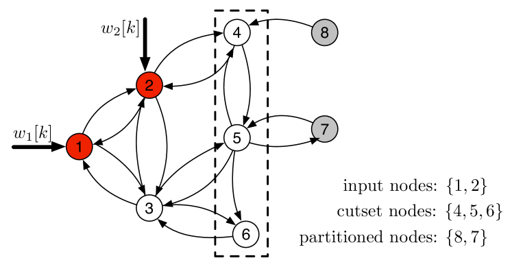
In this paper, we show that the graphical proximity indeed modulate the MAP detector’s performance, for certain classes of the detection problems (2). In particular, we characterize networks for which the detection performance obtained when sensors are located on a node cutset is better (or worse) than the performance obtained when sensors are placed on nodes of the subnetwork induced by the node cutset that does not contain the input nodes (precise statements are provided in Section 4). See Fig 1 for an illustration of node cutset and the subnetwork (partitioned nodes) induced by it.
Throughout the paper, we will distinguish the performance of sensors with measurement noise and without noise . The essential reason, as we will show later, is that only in the presence of noise, we have a scenario where the performance of a MAP detector associated with the cutset nodes may be worse than that of the partitioned nodes. We end this section with an example that shows the impact of noise on the detection performance.
Example 1
Let and , where is the tuning parameter and . For , the MAP detector’s error probability, based on samples of , is . Here denotes the SNR, and is decreasing in . For , the error probability does not depend on , and is lesser than the case where . However, when , depends on . In particular, when is small, is high, and vice versa. Thus, in the presence of noise, the error probability can be reduced by properly tuning .
3 Detection performance of the MAP detector
In this section, we derive the algebraic expressions of the MAP decision rules and their error probabilities for two special cases of the hypotheses in (2). The first case is the mean shift model, in which the covariance matrices in (2) are equal, but the mean vectors are different. The MAP detector (see (9) for the decision rule) for this case is the optimal detector in the (Bayesian) sense that, for the simple hypotheses and defined as in (2), no other detector outperforms the detection performance of (9). The second case is the covariance shift model in which the mean vectors in (2) are equal, but the covariance matrices are different. For this latter case, we will rely on the sub optimal LD-MAP detector (see below) for deciding the hypothesis. The reason for working with these models is twofold: (i) the error probability expressions are analytically tractable and (ii) these models are widely used for detection and classification problems that arise in practice [18, 19]. The probability expressions derived in this section will be used for the network analysis of the MAP detector’s performance (Section 4). Our work draws on the extensive literature on hypothesis testing using Multivariate Gaussian data, but uses a specific simplified detector which allows development of network-theoretic results. Extension of our framework and corresponding results to more general setting is mentioned in Remarks 2 and 3.
The results mentioned in the section are obtained from a standard application of hypothesis testing tools for linear models. Yet, to the best of our knowledge, the asymptotic characterization of the error probability of the MAP detector (Lemma 3.4) is novel, and it serves as the starting point for the results presented in the subsequent sections.
Definition 1
(Linear discriminant function-based MAP detector: LD-MAP) A LD-MAP detector is as in (5) with (4) replaced by the discriminant function , where the vector 333In the literature of pattern recognition and communications, is commonly referred as to the Fisher’s discriminant and optimal SINR beam former, respectively [20, 21]. is the maximizer of the following information divergence criterion:
| (7) |
where is the density of given and .
Remark 1
We now state a lemma that provides us with the algebraic expressions of the MAP detectors associated with the mean shift model, and the LD-MAP detector associated with the covariance shift model.
Proposition 3.1
Lemma 3.2
(MAP detectors) Let and be non-zero priors, and define . Let be as in (4), and let and be as in (2) and (8), resp.
-
(i)
The MAP detector associated with the mean shift model ( but ) is given by:
(9) where and .
-
(ii)
The LD-MAP detector associated with the covariance shift model ( but ) is given by:
(10) where , , and .
The detectors (9) and (10) are functions of the sufficient statistics and , respectively. This means that, given these statistics, other information in is not needed for deciding between and . In order to characterize the error probabilities of the detectors in Lemma 3.2, we make the following assumption:
Assumption 3.3
The LTI system (1) is stable. Further,
-
(i)
for the mean shift model, , where , and for some , and
-
(ii)
for the covariance shift model, and .
Lemma 3.4
The assumptions and are for the ease of presentation, and the probability expressions can be easily adjusted to include other priors and initial conditions. The assumption ensures that . Instead, the assumption is to eliminate the remainder terms in the computation of . We emphasize that the only restriction on is that it should be finite, but can be arbitrarily large. We now state a corollary to the above lemma in which we do not assume in the covariance shift model (see Remark 2).
Corollary 3.5
(SNRs: identical input statistics) Let in (2) be , where and are scalars, and . For the covariance shift model let . Then,
| (15) | ||||
| (16) |
where , , , and .
The error probabilities for the identical statistics case can be obtained by substituting and to and in (11) and (12), respectively. The effect of sensor noise is also evident from the SNR expressions in the above corollary. In particular, by setting in (15) and (16), the probabilities do not depend on the network matrix .
Notice that the expressions of and in above lemma are valid even when is finite. However, in this case, and are complicated functions of the adjacency matrix . Instead, the elegance of SNRs in Lemma 3.4 and Corollary 3.5 is that they depend on the adjacency matrix through the well understood transfer matrix . Thus, when , one can easily understand the impact of network structure on the detection performance by analyzing . By interpreting the quadratic function in (or ) and in (or ) as a measure of gain, one expects that higher gains results in minimum error probabilities. This intuition is made precise in the following proposition:
Proposition 3.6
and are decreasing in the SNRs (or ) and (or ), respectively.
The above proposition also helps us to compare the performance of the MAP and LD-MAP detectors associated with different sensor sets. This fact will be exploited greatly in the next section.
Remark 2
(LD-MAP detector’s error probability for other covariance matrix structures) We now comment on extending (12) for including other covariance matrices. The case and can be handled using the proof of Lemma 3.4. For the scenario where neither of or is zero, if we have and , then remains the same as in (12), with . For other cases we refer the reader to [19]. However, the main difficulty in analyzing any of these error probabilities lies in the fact that resulting expressions of SNRs () are not amenable to analysis. If one assumes and to be simultaneously diagonalizable, as is the case with Corollary 3.5, an expression of similar to (16) may be obtained.
4 Network analysis of the MAP detector
In this section, we characterize networks for which the MAP detector’s performance associated with the sensors that are close to the input nodes is better (or worse) than those of sensors that are farther apart. We distinguish two separate cases when the sensors are without noise () and with noise (). To make the notion of closeness precise, we introduce the notion of a node cutset.
Definition 2
(Node cutset) For the graph with input nodes , the nodes , with , form a node cutset if there exist a non empty source set and a non empty partitioned set such that , where denotes the disjoint union, and
-
(i)
and , and
-
(ii)
every path from to contains a node in .
The requirement (i) ensures that the node cutset is at least edges away from the input nodes. To illustrate Definition 2, consider the network in Fig 1. For the input nodes , the nodes forms a node cutset. However, the nodes ceases to form a node cutset, since they failed to satisfy requirement (ii) in the above definition.
4.1 Noiseless measurements
In this section, we state our results on network theoretic characterization of the MAP detectors assuming that the measurement noise in (1) is negligible, i.e., . It should be noted that, if a result holds true for the general detection problem (2), we do not state the analogous result for the mean and covariance shift models.
Theorem 4.1
(Performance of sensors on the node cutset vs the partitioned set: noiseless measurements) Consider the general detection problem (2). Let and be as in Definition 2, and assume that the measurements from both these node sets are noiseless (). Associated with these measurements, let and be the respective error probabilities that are computed using (6). Then, .
This comparison result is a mere consequence of the following well known result in the binary hypotheses detection problem, known as theorem of irrelevance [22] and the invariance of MAP decision rule [23].
Lemma 4.2
(Error probability of the MAP detector: dependent measurements) Let and be any two arbitrary simple hypotheses with non-zero priors. Let be the error probability of a MAP detector relying on the measurement , and be such a quantity associated with the measurement , where and is stochastically independent of the hypotheses. Then, .
From Lemma 4.2, it also follows that Theorem 4.1 holds true even (i) for the case of non-Gaussian input and measurements (provided that the joint density exists), and (ii) if the set is replaced with , where .
Theorem 4.1 implies that, in the absence of noise, nodes near the input location achieve better detection performance compared to those far away from the inputs, irrespective of the edge weights in the adjacency matrix and the measurement horizon . Here, the notion of closeness is to be understood in the sense of node cutsets, since, . Thus, if node cutsets exist in a graph and the measurements are noiseless, one should always place sensors on the cutsets. Thus, if a budget is associated with the sensor placement, it makes sense to find a cutset of minimum cardinality.
Proposition 4.3
(Error probability of the oracle detector) Consider the general detection problem (2), and let be the error probability of a MAP detector which can directly access the inputs , . For any sensor set , let and be the error probabilities associated with the noiseless and noisy measurements (4), respectively. Then, .
Proposition 4.3 states that sensor noise degrades the performance of the MAP detector (this fact is also illustrated in Example 1). It also implies that measuring the inputs directly is always better than measuring the noisy/noiseless states (dynamics) of the nodes. Of course, given this fact, it is always beneficial to place the sensors at the input nodes, rather than dealing with the node cutsets and the partitioned sets.
4.2 Noisy measurements
We now consider the case of noisy measurements (). Notice that our results will be specific to the MAP and LD-MAP detectors associated with the mean and covariance shift models, respectively. Possible extensions to the general detection problem (2) are mentioned in the remarks. We now introduce some additional notation. For a cutset , let , , and denote the states of the node sets , , and , respectively. Let be a permutation matrix such that , where is the state vector of (1). Then, from (1) it also follows that
| (17) |
From the above relation, note that the states of serve as an input for the states of partitioned nodes set , i.e.,
| (18) |
Based on the transfer function matrix of subsystem (18), we now state a result that is analogous to Theorem 4.1, for the case .
Theorem 4.4
(Performance of sensors on the node cutset vs the partitioned set: noisy measurements) Let and be as in (17), and assume that . Let and be the maximum and minimum singular values of , respectively. Let in (11) and in (12) be the error probabilities obtained using the noisy measurements () from the cutset . Instead, let and be the error probabilities associated with the partitioned set . Then we have:
-
1a)
If , then .
-
1b)
If , then .
-
2a)
If then .
-
2b)
If , then .
Hence, in the presence of noise, depending upon the entries in the matrix , measuring the cutset might not be always optimal for the purposes of the detection. Instead, in the noiseless case, Theorem 4.1 states that measuring the cutset is always optimal, irrespective of the entries in . We now explain the reason behind this contrasting behaviors.
Notice that, the quantities and of and in Theorem 4.4, respectively, are the maximum and minimum input to output gains of the transfer function matrix , associated with the system (18). Theorem 4.4 says that, if the gain between the states and the states is high (low), the detection performance with sensors in should be better (worse) that that of . In fact, recall from Lemma 3.4 that the detectors associated with the noisy measurements of and , respectively, depends on the SNRs of and (plus the sensor noise), respectively. Since , it is clear that the SNRs are influenced by the gains of . In particular, a higher gain increases the SNR of the detector associated with , which results in a better performance compared to the detector associated with that of .
The above reasoning also holds in the case of noiseless measurements, however, the transfer function gain do not influence MAP detector’s performance. In fact, this gain gets canceled in the error probability computations (this can be clearly seen in Example 1 by interpreting as the gain). Theorem 4.4 provides conditions for placing sensors on or away from the cutset nodes. For general adjacency matrix, one needs to rely on the software (based on LMI based inequalities) to validate those conditions. However, for non-negative adjacency matrices, the conditions for placing (or not) sensors on the cutset nodes can be stated based on algebraic conditions on the entries of the adjacency matrix. In fact, we have the following result:
Lemma 4.5
The inequality can be obtained even without the non-negativity assumption on . However, this might not be true for the case of . Thus, by ensuring that the maximum row sum of is bounded by (here refers to the cardinality of the partitioned set ), one can guarantee that the detection performance of sensors on the cutset is always superior than that of the sensors on the partitioned nodes. The assumption in part 2) of above lemma implies that . For arbitrary , the condition row sums of greater than one may not be sufficient, and more assumptions on are required to handle this case. For instance, when is a diagonally dominant matrix, required sufficient conditions can be obtained using the lower bounds in [24]. Finally, we notice that the bounds presented in Lemma 4.5 depends on the cardinality of the node sets, and hence, our results on networks with non-negative edge weights may be conservative when these cardinalities are large.
The network-theoretic analysis of the MAP and the LD-MAP detectors developed in this section can also be used to inform the placement of sensors for detection. The results show that sensors placed close to the stochastic inputs are effective for batch detection. More precisely, measurements on separating cutsets of the network necessarily outperform downstream sensing strategies. Thus, a strategy for the placement of few sensors is to find small node cutsets that isolate the input nodes. The design of these algorithms falls outside the scope of this paper and is left as the subject of future research.
Remark 3
(Extension of network theoretic results to the other detectors: noisy measurements) In the cases where the analytical error probability calculation is difficult, eg., the general Gaussian or non-Gaussian detection problem and the covariance shift model with arbitrary covariance matrix structures, one relies on the Chernoff type bounds (for eg., see [18]) to quantify the detection performance. In both the cases, i.e., evaluating the performance directly or via bounds, Theorem 4.4 holds true for any detector whose performance (resp. bounds) is monotonically increasing in , for some suitable . For instance, the Chernoff bounds on the error probability of the general Gaussian detection problem (2) depend on the moment generating function (mgf) of the sufficient statistic of the MAP detector, which ultimately depends on the filtered mean and covariance matrices (8), and our analysis becomes applicable. In the non-Gaussian case, the mgf might depend on other moments as well, and extending our analysis to this case will be challenging.
4.3 Single input single output (SISO) line networks
In this section, we validate our cutset based results, that we presented in previous section, for the case of line networks by explicitly expressing the error probabilities as a function of the entires of , and then compare the performance of sensors on versus sensors on . We restrict our attention to the SISO systems.
We assume that a stochastic input enters the network through a fixed node , and we allow any node with for sensor placement. For this setup, we assume that probabilities and are obtained by substituting the SNRs (15) and (16) in the expressions of (11) and (12), respectively. Notice that, in contrast to the previous analysis, in which we assume (see Assumption 3.3), in this section we do not assume in . For the ease of presentation, we assume the cutset to be a singleton set, i.e., . The following proposition is an extension of Lemma 4.5 for our SISO system setup with the revised error probabilities.
Proposition 4.6
Let be as in Lemma 4.5, and . Let and be the cutset and partitioned sets, resp. If , then for any , we have and . The opposite inequality holds true if all row sums of are greater than one.
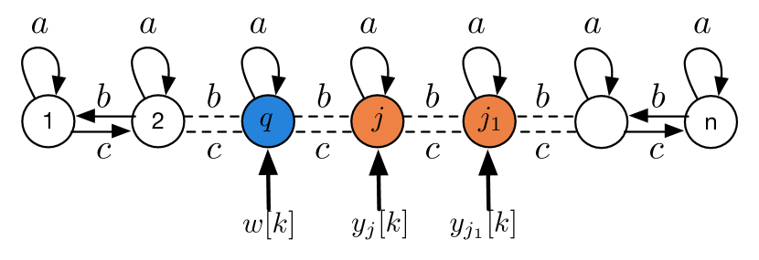
The proof of above proposition is similar to the proof of Lemma 4.5 and hence, the details are omitted. By not resorting to any proof techniques, i.e, the functional dependence arguments, that we used in previous section, we now validate assertions in above proposition by expressing the error probability in terms of the entries in the matrix . To this aim, we consider a line network (see Fig. 2), whose adjacency matrix is given by the following matrix:
| (19) |
where, . We let the cutset node be located on the right of the input node , i.e., (see Fig 2). The case when is to the left side of the input node follows similar analysis. Thus, we have the partitioned set . We now show that, for any , the error probabilities and are greater or smaller than those of the cutset node . The following proposition helps us achieve the required goal:
Proposition 4.7
For a fixed input , above proposition characterizes the qualitative behavior of the input-to-output transfer function gains associated with different output nodes. This fact can be easily seen by expressing as . For the case of Toeplitz line networks, the assertion in Proposition 4.6 is now an easy consequence of Proposition 3.6 and 4.7. In particular, if and , Proposition 4.7 also implies that, the node that is farthest from the input has better detection performance than any other node, including the cutset node. Similarly, assertion in Theorem 4.1 can be verified by letting .
The procedure illustrated above, evaluating the error probabilities via the entries of , becomes tedious and might not be even possible for arbitrary network structures. In such situations, one can use the proof techniques presented in Section 4 for understanding the detection performance of sensors on networks.
5 Simulation results
In this section, we present numerical simulations to validate the effectiveness of our cutset based characterization of MAP detection performance on networks, for the case of noisy measurements.
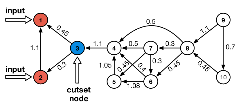
(Detection performance of sensors on the partitioned nodes is better than that of the sensors on the cutset nodes): For this scenario, consider the network in Fig 3. The network has 10 nodes, with and being the input nodes, is the cutset node, and is the partitioned node set. The adjacency matrix of this network is nilpotent, and as a result, system (1) evolving on this network will have a short memory (in fact ). By short (resp. long) memory, we mean that the current state of the network depends on few (resp. several) past states. For the mean shift model, the input , where , , and . Instead, for the covariance shift model, the input444the choice of zero mean is arbitrary, since, the LD-MAP detector’s error probability do not depend on the mean; see Lemma 3.4. , where and . In both the models, and the sensor noise variance .
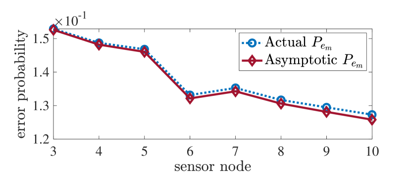
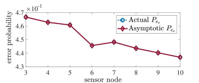
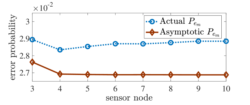
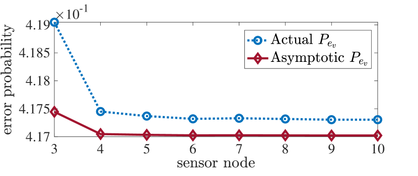
Fig. 4(a) and Fig. 4(b) illustrates the actual and asymptotic error probabilities of the mean and covariance shift models, respectively. The error probabilities are computed using the formulas in Lemma 3.4. In particular, for the asymptotic case, we use the SNRs in Corollary 3.5. In both figures, the error probability associated with the cutset node is greater than that of any node in the partitioned set. This must be the case since , and the row sums of the submatrix are greater than one (see Lemma 4.5).
The error between the asymptotic and actual error probabilities in Fig. 4(a) and Fig. 4(b) is almost negligible, even when is not large. This is because the adjacency matrix is a nilpotent matrix, and as a result, the difference between the actual and asymptotic SNRs is minimum. However, this might not be the case when has long memory, i.e., only for a very large . For , Fig. 4(c) and Fig. 4(d) illustrate this scenario for the network that is obtained by modifying some edges of the network in Fig. 3, such that for very large .
(Detection performance of sensors on the cutset nodes is better than that of the sensors on the partitioned nodes):
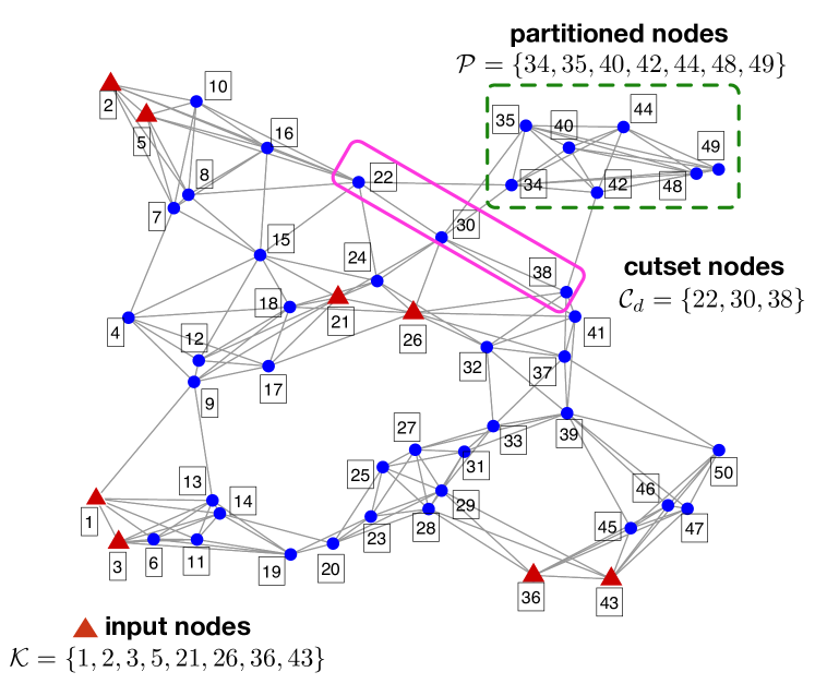
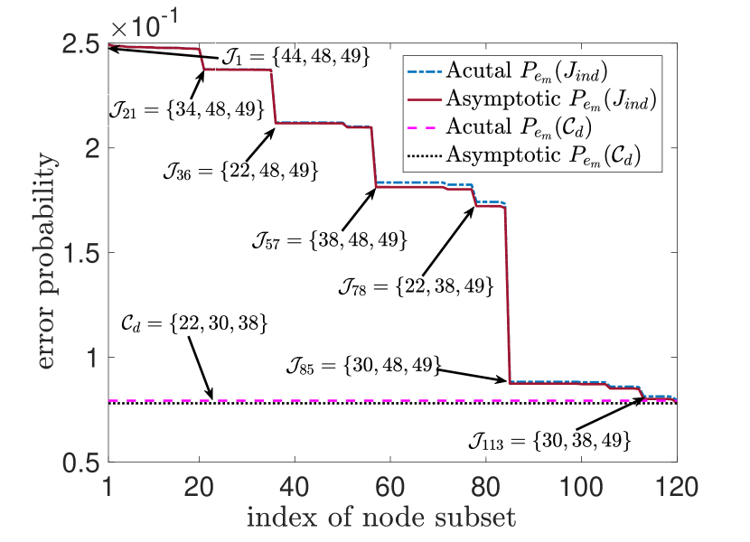
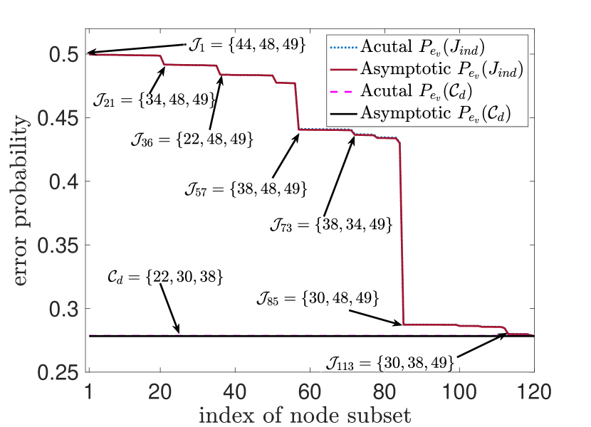
Consider the network shown in Fig 5. The network has 50 nodes among which are the input nodes. The cutset separates from the partitioned set . For the mean shift model, the input , where , , and , and . Instead, for the covariance shift model, the input , where , , and . In both the models, .
Consider all possible subsets of whose cardinalities are same as that of the cutset . It is easy to see that there are such sets. For each of these sets, we associate a label , where . The labels are given based on a decreasing order of the error probabilities associated with the subsets. In Fig. 6(a) and Fig. 6(b), we show the actual and asymptotic error probabilities of the mean and covariance shift models, respectively. In both figures, the error probability associated with the is lesser than that of any . This must be the case because , and the row sums of the submatrix (see Lemma 4.5).
6 Conclusion
In this paper we formulate mean and covariance detection placement problems for linear dynamical systems defined over networks with unknown stochastic inputs. The main technical contribution of the paper is to identify graphical conditions that predict the performance of MAP and LD-MAP detectors based on the distance between the employed sensors and the stochastic inputs. For networks with non-negative edge weights, we also show that the performance of a detector can be independent of the graphical distance between the sensors and the stochastic inputs.
APPENDIX
Proof of proposition 3.1: From the network dynamics (1) and sensor measurements (3), (4) can be expanded as
| (20) |
where the vectors and , respectively. The matrices and are defined in the statement of the proposition. The expressions of and in (8) follows by taking the expectation and covariance of , respectively.
Proof of Lemma 3.2: Let and are the realizations of and , respectively. Since the input and measurement noises follows a Gaussian distribution, the probability density functions of (4) and are
| (21) |
respectively, where denotes the determinant. Define the log likelihood ratios and . Then, from the mixed Bayes formula [23], the MAP decision rules based on and , respectively, are given by
| (22) |
part 1) Since and , from (8), it follows that and . Invoking this observation in , yields the following expression for :
| (23) |
Substitute (23) in the first decision rule of (22) and simplify the resulting expression to obtain the MAP decision rule (9) for . Finally, replacing with yields the required expression.
part 2) In this case we have and . A similar procedure, as in part 1), based on (22) and the second decision rule in (APPENDIX), yields the LD-MAP detector’s expression (9). Details are left to the reader.
Proof of Lemma 3.4: We divide the proof into two parts. In part 1) we derive the expressions (11) and (13) Instead, in part 2) we derive the expressions (12) and (14).
part 1) Under the assumption that , let be the error probability of (9).. Then, from (9), we have
where follows under , because is a linear transform of , which follows a Gaussian distribution. Define , and notice that and . Finally, from (6), we have . Define , and note the following:
where the final equality follows because is increasing in (see Proposition A.1). We now show that . From (8), it follows that
| (24) |
where and . Let , and define and . With these definitions and the assumption , we have , and
| (25) |
Let . By substituting (25) in (24), we have
| (26) |
Consider the first term of (26). Since , from (8), it follows that . Further,
| (27) |
where is obtained by permuting, bottom to top, the block matrices of (25). Right multiplying either sides of (APPENDIX) with gives us:
| (28) |
where and is defined in (26). Since , from (28), it follows that . Substituting in (26) yields
where . Finally, substituting in the above expression, and manipulating the terms will give us
| (29) |
We claim that . To see this, rewrite as , where
From part 1) of Assumption 3.3, there exist a such that for all , . Thus, all but finite rows of (25) are zeros, i.e., we can express as and as , where the dimension of and depends only . Thus, for all , is a constant matrix, say , and we may conclude that
where and are the maximum and minimum eigenvalues. Since (Assumption 3.3), it follows that . Hence, and (13).
part 2) Under the assumption that , let be the error probability of (10). Then, from (9), we have
where and (since ; Assumption 3.3). Let . Then, , where means equality in the distribution. From this fact, we now have and , where . Since , we finally have
To simplify , note the following: since is the maximizer of -divergence (7), from [19], we can also express as
Let , and note the following:
Since is an increasing sequence, with respect to (see Proposition A.1), the limits , and are well defined. Now, consider
where the last equality follows because and are decreasing and increasing in (Proposition A.1), resp.
We now show that is given by (14). Since and , we have and , where and satisfies . From these observations, we may conclude that
| (30) |
It now suffices to evaluate . Since , we may define the following matrix valued function [26]:
where and . Since the coefficients are absolutely summable, for any , these coefficients can also be recovered as [26]:
Let be the conjugate of . Then, from [27, Chapter 6.4], we have
where follows because, for any with denoting its complex conjugate transpose, . Substituting in (APPENDIX) gives us .
Proof of Theorem 4.1 Let and denote the measurements of associated with the sensor sets and , respectively. Since , from (18), we have
| (31) |
where . From (31), it follows that
Since is independent of , the assertion of the theorem follows from Lemma 4.2.
Proof of Lemma 4.2 We shall prove the result assuming that and admits density functions. With the expense of notation, the given proof can be adapted to handle random variables that do not have densities. Let . Consider the following log likelihood ratio (LR) based on :
where (a) follows because is independent of . Since LRs of and are equal, the error probabilities associated with their MAP rules should be the same. Instead, the error probability of the MAP rule based on is always superior to that of or alone. Thus .
Proof of Theorem 4.4 Consider the following deterministic analogue of (1): , where is arbitrary. Recall that (18). Since , for , we have
| (32a) | |||
| (32b) |
From (32b), the following inequalities are obvious
| (33) |
Let and be the sensor matrices associated with and , respectively. Then,
| (34) |
part 1) We now consider the cases 1a) and 1b). Let , where is defined in Lemma 3.2. Let . Then, from (34) note that
From (33) and above identities, it follows that
| (35) | ||||
Let , where is defined in the statement of Lemma 3.4. Let and be the SNRs of and , respectively. Then from (13), we have
Using the identity , we can also express as
| (36) |
Finally, from (36) and (35), and Proposition 3.6, we have
part 2) We now consider the cases 2a) and 2b). Let . Let , where is defined in the statement of Lemma 3.4. From (34) and (32a), we have and . By invoking these two facts in (33), we may now conclude that
for all that satisfies . Let and be the SNRs of and , respectively. Then, from (14)
From Proposition 3.6, it follows that
Proof of Corollary 4.5 We shall prove part 1) of the corollary, and part 2) can be derived using similar analysis (the details are omitted). The idea of the proof is to show that , and there upon invoking Theorem 4.4 yields the desired assertion.
step 1) For , it follows that , where is . To see this, note the following: For any , let . Then, for any and that satisfies , we have
where the inequality, to be understood coordinate wise, follows because . From the above inequality, and the fact for any , we have
Since is a submatrix of , which is a non-negative matrix, we have [28], the above inequality can also be expressed as
Taking -norm on both sides of the inequality yields us:
Since the above inequality holds for any vector , using the identity for any , the following inequality is now obvious:
which can be expressed as . The equality is attained at .
step 2) Since , from Theorem 4.4 it readily follows that, both and holds true whenever . We now show that guarantees . Let denote the all ones vector, and note the following identity:
| (37) |
Since , for any , we also have
From the above inequality and (37), it follows that
Since , as , it follows that and . Thus , and hence, .
Proof of Proposition 3.6 Since is decreasing function of , (11) is decreasing in SNR , given by either (13) or (15). For (12) note the following: first, observe that in both (14) and (16). Thus
| (38) | ||||
Hence, we conclude that is deceasing in . Instead, is increasing in . From this observation and the fact that the , where , is decreasing in , it follows that is decreasing in .
Proof of Proposition 4.7 From (19), and the fact that , where and , the row sums of takes values in the set . Let . Using the principle of backward induction, we shall show that, when , is monotonically decreasing. The proof of part (ii) is left to the reader as an exercise.
Let , , . If , then of are given by the following expressions [29]:
| (41) |
where , and and are governed by
| (42) | ||||
where , , , and . Let . Then, for any ,
Let , and define . Since and , for (base step), it follows that
where follows because , and . Let and (inductive step). Then,
To see the last inequality, consider the following:
where follows because the hypothesis implies that , and from the fact that , , and . From the principle of finite induction, for all , we have . Hence, is a decreasing sequence.
Proposition A.1
Let , and , where (, , , ) are defined in the statement of Lemma 3.2. Then, , , and are increasing in . However, is decreasing in .
Proof: Let . Then, from Proposition 3.1, we have , . For clarity, we drop the existing subscripts and replace them with the total number of measurements. Let , , and consider , where are the measurements collected after . Then,
where , , and . Further, using the Schur complement, can be expressed as
From the above identity, it follows that
Hence, we may conclude that is increasing in . Instead, from the eigenvalue interlacing property for the symmetric matrix pencils [30], it follows that is increasing in . Finally, from (38), it follows that and are decreasing and increasing in , respectively.
References
- [1] F. Pasqualetti, F. Dörfler, and F. Bullo. Attack detection and identification in cyber-physical systems. IEEE Transactions on Automatic Control, 58(11):2715–2729, Nov 2013.
- [2] H.S. Sánchez, D. Rotondo, T. Escobet, V. Puig, and J. Quevedo. Bibliographical review on cyber attacks from a control oriented perspective. Annual Reviews in Control, 48:103 – 128, 2019.
- [3] S. Roy, J. Abed Torres, and M. Xue. Sensor and actuator placement for zero-shaping in dynamical networks. In 2016 IEEE 55th Conference on Decision and Control (CDC), pages 1745–1750, Dec 2016.
- [4] L. Ye, S. Roy, and S. Sundaram. On the complexity and approximability of optimal sensor selection for kalman filtering. In 2018 Annual American Control Conference (ACC), pages 5049–5054, June 2018.
- [5] R. Dhal, J. Abad Torres, and S. Roy. Detecting link failures in complex network processes using remote monitoring. Physica A: Statistical Mechanics and its Applications, 437:36 – 54, 2015.
- [6] R. Anguluri, R. Dhal, S. Roy, and F. Pasqualetti. Network invariants for optimal input detection. In 2016 American Control Conference (ACC), pages 3776–3781, July 2016.
- [7] S. Roy, M. Xue, and S. Sundaram. Graph-theoretic analysis of estimators for stochastically-driven diffusive network processes. In 2018 Annual American Control Conference (ACC), pages 1796–1801, June 2018.
- [8] Y. Liu, J. J. Slotine, and A. L. Barabási. Observability of complex systems. Proceedings of the National Academy of Sciences, 110(7):2460–2465, 2013.
- [9] A. Vosughi, C. Johnson, M. Xue, S. Roy, and S. Warnick. Target control and source estimation metrics for dynamical networks. Automatica, 100:412–416, 2019.
- [10] T. H. Summers, F. L. Cortesi, and J. Lygeros. On submodularity and controllability in complex dynamical networks. IEEE Transactions on Control of Network Systems, 3(1):91–101, March 2016.
- [11] H. Zhang, R. Ayoub, and S. Sundaram. Sensor selection for kalman filtering of linear dynamical systems: Complexity, limitations and greedy algorithms. Automatica, 78:202–210, 2017.
- [12] J. Abad Torres, S. Roy, and Y. Wan. Sparse resource allocation for linear network spread dynamics. IEEE Transactions on Automatic Control, 62(4):1714–1728, April 2017.
- [13] F. Pasqualetti, S. Zampieri, and F. Bullo. Controllability metrics, limitations and algorithms for complex networks. IEEE Transactions on Control of Network Systems, 1(1):40–52, March 2014.
- [14] S. Zhao and F. Pasqualetti. Discrete-time dynamical networks with diagonal controllability gramian. IFAC-PapersOnLine”, 50(1):8297–8302, 2017. 20th IFAC World Congress.
- [15] H. J. Van Waarde, M. K. Camlibel, and H. L. Trentelman. A distance-based approach to strong target control of dynamical networks. IEEE Transactions on Automatic Control, 62(12):6266–6277, Dec 2017.
- [16] I. Gohberg, A. M. Kaashoek, and S. Goldberg. Block toeplitz operators. In Classes of Linear Operators Vol. II. Birkhäuser Basel, 1993.
- [17] J. Abed Torres and S. Roy. Graph-theoretic analysis of network input-output processes: Zero structure and its implications on remote feedback control. Automatica, 61:73–79, 2015.
- [18] H. L. Van Trees. Detection, Estimation, and Modulation Theory. Part I:. Wiley Press, 2004.
- [19] L. L. Scharf. Statistical Signal Processing. Reading, MA: Addition-Wesley, 1991.
- [20] R. Duda, P. Hart, and D. Stork. Pattern Classification. New York: Wiley, 2000.
- [21] Y. Bresler, V. U. Reddy, and T. Kailath. Optimum beamforming for coherent signal and interferences. IEEE Trans. on Acou., Speech, and Signal Process., 36(6):833–843, June 1988.
- [22] J. M. Wozencraft and I. M. Jacobs. Principles of Communication Engineering. New York: Wiley, 1965.
- [23] J. L. Melsa and D. L. Cohn. Decision and Estimation Theory. McGraw-Hill, 1978.
- [24] J. M. Varah. A lower bound for the smallest singular value of a matrix. Linear Algebra and its Applications, 11(1):3–5, 1975.
- [25] N. Perraudin, J. Paratte, D. Shuman, L. Martin, V. Kalofolias, P. Vandergheynst, and D. K. Hammond. Gspbox: A toolbox for signal processing on graphs. ArXiv e-prints, Aug. 2014.
- [26] R. M. Gray. Toeplitz and circulant matrices: A review. Foundations and Trends® in Communications and Information Theory, 2(3):155–239, 2006.
- [27] A. Böttcher and B. Silbermann. Block toeplitz matrices. In Introduction to Large Truncated Toeplitz Matrices, pages 185–219. Springer New York, 1999.
- [28] A. Berman and R.J. Plemmons. Nonnegative Matrices in the Mathematical Sciences. Society for Industrial and Applied Mathematics, 1994.
- [29] J. W. Lewis. Inversion of tridiagonal matrices. Numerische Mathematik, 38(3):333–345, Oct 1982.
- [30] R. C. Li. Rayleigh quotient based optimization methods for eigenvalue problems. In Matrix Functions and Matrix Equations, pages 76–108. World Scientific, 2015.