Model Reduction Framework with a New Take on Active Subspaces for Optimization Problems with Linearized Fluid-Structure Interaction Constraints

Abstract

[Summary]In this paper, a new take on the concept of an active subspace for reducing the dimension of the design parameter space in a multidisciplinary analysis and optimization (MDAO) problem is proposed. The new approach is intertwined with the concepts of adaptive parameter sampling, projection-based model order reduction, and a database of linear, projection-based reduced-order models equipped with interpolation on matrix manifolds, in order to construct an efficient computational framework for MDAO. The framework is fully developed for MDAO problems with linearized fluid-structure interaction constraints. It is applied to the aeroelastic tailoring, under flutter constraints, of two different flight systems: a flexible configuration of NASA’s Common Research Model; and NASA’s Aeroelastic Research Wing #2 (ARW-2). The obtained results illustrate the feasibility of the computational framework for realistic MDAO problems and highlight the benefits of the new approach for constructing an active subspace in both terms of solution optimality and wall-clock time reduction.

1 Introduction

Multidisciplinary analysis and optimization (MDAO) problems with fluid-structure interaction (FSI) constraints arise in many engineering applications including design and optimal control. Solving such problems requires repeated evaluations of the FSI constraints when using, for example, the nested analysis and design (NAND) approach. Typically, each evaluation of FSI constraints incurs the solution of some coupled computational fluid dynamics (CFD) - computational structural dynamics (CSD) problems. In an industrial setting, these CFD-CSD problems are usually large-scale when high-fidelity simulations are required. Furthermore, the number of solutions of coupled CFD-CSD problems increases when the design parameter space $\mathcal{D}$ is high-dimensional. This is because the number of evaluations of the objective function and constraints incurred by an MDAO problem generally increases with the dimension $N_{\mathcal{D}}$ of $\mathcal{D}$. For all these reasons, solving highly parameterized, FSI-constrained, MDAO problems can be very computationally intensive. Consequently, the main objective of this paper is to present an innovative, comprehensive, computational framework for efficiently solving such problems when the FSI constraints are linearized in the spatial, temporal, or frequency domain. Such linearizations are common when the FSI constraints pertain to stability or control problems.

The computational cost of a linearized, coupled FSI problem can be reduced by substituting the underlying coupled high-dimensional model (HDM) with a less computationally intensive surrogate model such as a linear, coupled, projection-based, reduced-order model (PROM). Such a linear PROM can be local (or pointwise), or global. In the context of this paper, the label local describes a PROM that was trained at a single parameter point $\boldsymbol{\mu}\in{\mathcal{D}}\subset{\mathbb{R}}^{N_{\mathcal{D}}}$ of the design parameter space $\mathcal{D}$. On the other hand, the label global refers to a PROM that was trained at multiple points in $\mathcal{D}$ so that it is robust and accurate within a large region of this parameter space.

The overhead cost – also known as the offline cost – associated with the construction of a local PROM is lower than that associated with the construction of a global PROM, given that it involves training at a single parameter point. Unfortunately, a local PROM does not usually perform well away from the training point. Therefore, it is not suitable for the solution of an MDAO problem unless it is reconstructed everytime a new parameter point is queried, which is inefficient. Alternatively, a global PROM may be suitable for MDAO problems, from the robustness and accuracy viewpoints. However, such a PROM is bound to be of a larger dimension than needed at any parameter point visited online by the optimization trajectory, given that it was trained offline at multiple points of the parameter space; this also hinders computational efficiency.

In order to overcome the inefficiency issues highlighted above, different approaches have been proposed in the literature. In the context of linear PROMs, two of them are noteworthy. First, the adaptive approach consisting in progressively updating an initial PROM by continuously training it at a subset of the parameter points previously visited by the optimization trajectory ¹. In this approach, which breaks the traditional offline-online framework of model order reduction, the reduced optimization problems are equipped with a nonlinear trust-region based on a residual error indicator to keep the optimization trajectory in a region of $\mathcal{D}$ where the PROM is accurate. Hence, whereas this approach is equally applicable to linear PROMs, it was designed primarily for nonlinear PROMs. The second approach consists in carefully sampling the parameter space $\mathcal{D}$ at a small set of points, constructing at each sampled parameter point a local PROM, and storing in a database all constructed local PROMs as well as some related quantities such as the underlying reduced-order bases (ROBs) ². This approach is natural for linear PROMs as once the database has been constructed offline, a linear PROM – as well as its sensitivities – can be constructed in real-time at any unsampled parameter point queried by the optimization trajectory using interpolation on matrix manifolds ³. This approach has been recently demonstrated for MDAO problems characterized by a small-dimensional design parameter space – say $N_{\mathcal{D}}\leq 6$ – and shown to deliver excellent speedup factors. For high-dimensional design parameter spaces however – say $N_{\mathcal{D}}\geq 10$, building a database of local PROMs suffers from the curse of dimensionality and rapidly becomes impractical if not infeasible. For example, sampling only 2 parameter points along each dimension of a design parameter space of dimension 10 leads to the construction of $2^{10}=1,024$ PROMs! Adaptive parameter sampling procedures – also known as greedy sampling (or simply greedy) procedures – and particularly those equipped with a saturation technique ⁴ attenuate somehow this issue but insufficiently. Alternatively, this paper addresses this issue by focusing on a PROM computational framework for MDAO where the concept adaptive parameter sampling, that of a database of linear PROMs, and a new take on the concept of active subspaces (AS) are intertwined.

The remainder of this paper is organized as follows. Section 2 formulates the problem of interest in sufficient details to keep this paper as self-contained as possible. Section 3 reviews and intertwines the concepts of AS, projection-based model order reduction (PMOR), and a database of linear FSI PROMs equipped with interpolation on matrix manifolds, in the context of MDAO problems with linearized FSI constraints. It also proposes an effective parameter sampling method for constructing an AS. Section 4 illustrates the proposed PROM-based computational framework for MDAO with the aeroelastic tailoring, under flutter constraints, of two different systems: a flexible configuration of NASA’s Common Research Model (CRM); and NASA’s Aeroelastic Research Wing ARW-2.

2 MDAO Problem with a Linearized FSI Constraint

2.1 Problem Formulation

The main focus of this paper is on the acceleration of the solution of MDAO problems under a high-dimensional, linearized, FSI constraint, as well as other linear or nonlinear constraints, including partial differential equation (PDE)-based constraints. Such problems can be written as

$$\boxed{\begin{aligned} &\underset{\textbf{q},\,\mathbf{z},\,\boldsymbol{\mu}}{\text{min}}&&f(\textbf{q},\mathbf{z},\boldsymbol{\mu})\\ &\text{s.t.}&&\mathbf{c}(\textbf{q},\mathbf{z},\boldsymbol{\mu}))&\leq&\,\boldsymbol{0}\\ &&&\mathbf{R}_{L}(\textbf{q},\boldsymbol{\mu})&=&\,\boldsymbol{0}\\ &&&\mathbf{R}_{NL}(\mathbf{z},\boldsymbol{\mu})&=&\,\boldsymbol{0}\\ \end{aligned}}$$ (1)

where:

• $f(\cdot)$ represents a scalar objective function to minimize.

• $\textbf{q}\in\mathbb{R}^{N_{q}}$ denotes a first high-dimensional vector of $N_{q}$ semi-discrete or discrete fluid and structural state variables involved in a high-dimensional, parametric, linearized, FSI constraint.

• $\mathbf{z}\in\mathbb{R}^{N_{z}}$ denotes a second high-dimensional vector of $N_{z}$ semi-discrete or discrete state variables involved in a high-dimensional, parametric, PDE-based constraint.

• $\boldsymbol{\mu}\in\mathcal{D}\subset\mathbb{R}^{N_{\mathcal{D}}}$ denotes a vector of $N_{\mathcal{D}}$ design optimization parameters and is assumed to be relatively large – say, $N_{\mathcal{D}}\geq 10$. Each component of this vector may represent some structural material property or an aerodynamic shape parameter.

• $\mathbf{c}(\cdot)$ represents a general set of linear and nonlinear algebraic constraints.

• $\mathbf{R}_{L}(\textbf{q},\boldsymbol{\mu})$ is a high-dimensional, semi-discretized or discretized, parametric PDE that is linear in q, and the subscript $L$ designates the linear aspect.

• $\mathbf{R}_{NL}(\mathbf{z},\boldsymbol{\mu})$ is a high-dimensional, semi-discretized or discretized, parametric PDE that is nonlinear in $\mathbf{z}$, and the subscript $NL$ designates the nonlinear aspect.

Specifically, the focus is set on the gradient-based solution of the MDAO problem (1) using the NAND approach.

2.2 Nested Analysis and Design Approach

Two methodologies for solving MDAO problems such as (1) can be considered: Simultaneous Analysis and Design (SAND) and Nested Analysis and Design (NAND). In the SAND approach, both vectors of discrete state variables $\mathbf{q}$ and $\mathbf{z}$ as well as the vector of design parameters $\boldsymbol{\mu}$ are considered optimization parameters for problem (1). In this case, the MDAO problem has potentially millions of optimization parameters given the high-dimensionality of $\mathbf{R}_{L}(\textbf{q},\boldsymbol{\mu})$ and $\mathbf{R}_{NL}(\mathbf{z},\boldsymbol{\mu})$. In the NAND approach however, the only optimization parameters are the components of $\boldsymbol{\mu}$: in this case, $\mathbf{q}$ and $\mathbf{z}$ are recognized as implicit functions of $\boldsymbol{\mu}$ due to the constraints $\mathbf{R}_{L}(\textbf{q},\boldsymbol{\mu})=\boldsymbol{0}$ and $\mathbf{R}_{NL}(\mathbf{z},\boldsymbol{\mu})=\boldsymbol{0}$. It follows that when storage is an issue, the NAND approach is preferrable. Furthermore, the NAND approach has the additional benefit or enabling the reuse of available solvers for the PDE-based constraints. For these reasons, it is here the method of choice.

Hence, problem (1) is rewritten as

$$\begin{aligned} &\underset{\textbf{q},\,\mathbf{z},\,\boldsymbol{\mu}}{\text{min}}&&f(\textbf{q},\mathbf{z},\boldsymbol{\mu})\\ &\text{s.t.}&&\mathbf{c}(\textbf{q},\mathbf{z},\boldsymbol{\mu})&\leq&\,\boldsymbol{0}\\ &&&\mathbf{R}_{L}(\textbf{q},\boldsymbol{\mu})&=&\,\boldsymbol{0}\\ &&&\mathbf{R}_{NL}(\mathbf{z},\boldsymbol{\mu})&=&\,\boldsymbol{0}\\ \end{aligned}\rightarrow\boxed{\begin{aligned} &\underset{\boldsymbol{\mu}\in{\mathcal{D}}}{\text{min}}&&f(\textbf{q}(\boldsymbol{\mu}),\mathbf{z}(\boldsymbol{\mu}),\boldsymbol{\mu})\\ &\text{s.t.}&&\mathbf{c}(\textbf{q}(\boldsymbol{\mu}),\mathbf{z}(\boldsymbol{\mu}),\boldsymbol{\mu})\leq\boldsymbol{0}\\ \end{aligned}}$$ (2)

Given at iteration $i$ of the NAND approach a queried parameter point $\boldsymbol{\mu}_{i}\in{\mathcal{D}}$, $\mathbf{R}_{L}(\textbf{q},\boldsymbol{\mu})=\boldsymbol{0}$ and $\mathbf{R}_{NL}(\mathbf{z},\boldsymbol{\mu})=\boldsymbol{0}$ are solved to obtain $\mathbf{q}(\boldsymbol{\mu}_{i})$ and $\mathbf{z}(\boldsymbol{\mu}_{i})$, and then the objection function $f$ and the set of algebraic constraints represented by $\mathbf{c}$ are evaluated. This process can be written as

$$\boldsymbol{\mu}_{i}\rightarrow\left\{\begin{aligned} &\mathbf{R}_{L}(\mathbf{q}(\boldsymbol{\mu}_{i}),\boldsymbol{\mu}_{i})&=&\,\boldsymbol{0}\\ &\mathbf{R}_{NL}(\mathbf{z}(\boldsymbol{\mu}_{i}),\boldsymbol{\mu}_{i})&=&\,\boldsymbol{0}\\ \end{aligned}\right.\rightarrow\left\{\begin{aligned} &\mathbf{q}=\mathbf{q}(\boldsymbol{\mu}_{i})\\ &\mathbf{z}=\mathbf{z}(\boldsymbol{\mu}_{i})\\ \end{aligned}\right.$$

Unfortunately, the number of solutions of the PDE-based constraints generally increases when the dimension of the design parameter space $\mathcal{D}$ is increased, which is a disadvantage of the NAND approach and a further motivation for model reducion.

2.3 Three-Field Linearized Computational Framework for FSI

The three-field framework pioneered in ⁵ is adopted for modeling a coupled FSI problem such as that represented here by $\mathbf{R}_{L}(\textbf{q},\boldsymbol{\mu})=\boldsymbol{0}$. In this framework, no limiting assumption is made about the behavior of the fluid subsytem whose governing equations of equilibrium are usually formulated in the Arbitrary Lagrangian Eulerian (ALE) setting and discretized by a CFD approach. Similarly, no limiting assumption is made about the behavior of the structural subsystem whose governing equations of equilibrium are formulated in the Lagrangian setting and discretized by a finite element (FE) method. The CFD mesh of the fluid subsystem is viewed as a third subsystem that is assimilated with a fictitious discrete structural system ⁶, or the FE discretization of a fictitious deformable continuous body ⁷ – so that it may move and/or deform as needed. In either case, it is referred to here as the pseudo-structural subsystem.

Most importantly, the three-field (fluid, fluid mesh, and structure) framework couples the fluid and structural subsystems by simply enforcing the kinematic transmission conditions expressing the slip or no-slip wall boundary conditions of the fluid subsystem, and the force transmission conditions expressing equilibrium at the fluid/structure interface. It is overviewed below with emphasis on the linearization of its semi-discrete form.

2.3.1 Three-field Formulation of FSI Problems

The three-field framework for computational FSI outlined above can be summarized by the following three equations

$$\left\{\begin{array}[]{l c l}\displaystyle{\frac{\partial(\mathcal{JW})}{\partial t}}+\mathcal{J}\nabla\cdot\left(\mathcal{F(W)}-\frac{\partial x}{\partial t}\mathcal{W}\right)-\mathcal{J}\nabla\cdot\mathcal{R(W)}&=&0\\[7.0pt] \displaystyle{\rho\frac{\partial^{2}\mathcal{U}}{\partial^{2}t}}-div\left(\sigma\left(\epsilon(\mathcal{U})\right)\right)-\mathcal{B}&=&0\\[7.0pt] \tilde{\rho}\displaystyle{\frac{\partial^{2}x}{\partial^{2}t}}-div\left(\widetilde{E}:\tilde{\epsilon}(x)\right)&=&0\end{array}\right.$$ (3)

where: the first equation is the Navier-Stokes equation written in ALE conservative form – and can be augmented with turbulence modeling; the second equation expresses the dynamic equilibrium of the structural subsystem; the third equation models the fluid mesh as a fictitious, dynamic, deformable body; and all dependences on the parameter point $\boldsymbol{\mu}$ have not been stated explicitly in order to keep the notation as simple as possible.

In the first of equations (3), $\mathcal{W}$ denotes the vector of conservative fluid variables, $x$ denotes the position vector of the fluid mesh, $\mathcal{J}$ is the determinant of the jacobian of $x$ with respect to the reference configuration of the fluid mesh, $t$ denotes time, $\nabla$ denotes the gradient with respect to $x$, $\cdot$ designates the standard dot product, $\mathcal{F}$ denotes the vector of ALE convective fluxes, and $\mathcal{R}$ denotes the vector of diffusive fluxes.

In the second of equations (3), $\mathcal{U}$ denotes the structural displacement vector, $div$ designates the divergence operator, $\rho$ denotes the material density, $\sigma$ denotes the stress tensor, $\epsilon$ denotes the strain tensor, and $\mathcal{B}$ is the vector of body forces acting on the structure.

In the third of equations (3), the symbols $\tilde{}$ and $\widetilde{}$ designate the fictitious aspect of the deformable body with which the fluid mesh is assimilated.

As already stated, the first two equations described above are coupled by the kinematic and equilibrium transmission conditions which have simple expressions that can be found, for example, in ⁸: therefore, they are not repeated here. Similarly, the second and third sets of equations are coupled by the continuity of the structural displacement and velocity fields across the fluid/structure interface.

Finally, each of equations (3) is equipped with its own boundary and initial conditions: these are not explicitly stated here for the sake of simplicity.

2.3.2 Semi-discretization

In this work, the fluid subsystem is semi-discretized by a finite volume (FV) method: however, it can be equally approximated by a FE method. On the other hand, the structural and pseudo-structural subsystems are semi-discretized by the FE method. In this case, the coupled FSI system (3) is transformed into

$$\left\{\begin{array}[]{l c l}\dot{\widehat{\left(\textbf{A}(\textbf{x})\textbf{w}\right)}}+\textbf{F}(\textbf{w},\textbf{x},\dot{\textbf{x}})-\textbf{F}^{\prime}(\textbf{w},\textbf{x})&=&\textbf{0}\\ \textbf{M}\ddot{\textbf{u}}+\textbf{ f}^{\,int}(\textbf{u},\dot{\textbf{u}})-\textbf{ f}^{\,ext}(\textbf{u},\textbf{w})&=&\textbf{0}\\ \widetilde{\textbf{K}}\textbf{x}-\widetilde{\textbf{K}}_{c}\textbf{u}&=&\textbf{0}\end{array}\right.$$ (4)

In the first of the above semi-discrete equations: $\mathbf{A}\in{\mathbb{R}}^{N_{f}\times N_{f}}$ denotes the diagonal matrix storing the cell volumes of the FV semi-discretization and $N_{f}$ denotes the dimension of the semi-discrete fluid HDM; $\mathbf{F}\in{\mathbb{R}}^{N_{f}}$ and $\mathbf{F}^{\prime}\in{\mathbb{R}}^{N_{f}}$ denote the vectors of semi-discrete convective and diffusive fluxes, respectively; $\mathbf{x}\in{\mathbb{R}}^{N_{m}}$ denotes the semi-discrete position vector of the fluid mesh and $N_{m}$ denotes the dimension of the associated HDM; $\mathbf{w}\in{\mathbb{R}}^{N_{f}}$ denotes the vector of semi-discrete conservative state variables of the fluid subsystem; and $\dot{()}$ denotes the first derivative with respect to time.

In the second of equations (4): $\mathbf{M}\in{\mathbb{R}}^{N_{s}\times N_{s}}$ denotes the usual mass matrix and $N_{s}$ denotes the dimension of the semi-discrete structural HDM; $\mathbf{f}^{\,int}\in{\mathbb{R}}^{N_{s}}$ and $\mathbf{f}^{\,ext}\in{\mathbb{R}}^{N_{s}}$ denote the vectors of semi-discrete internal and external forces, respectively; $\mathbf{u}\in{\mathbb{R}}^{N_{s}}$ denotes the vector of semi-discrete structural state variables (displacements and rotations); and $\ddot{()}$ denotes the second derivative with respect to time.

The third of the above equation is a quasi-static semi-discretization of the third of equations (3). In this equation, $\widetilde{\mathbf{K}}$ denotes the pseudo-structural stiffness matrix of the fluid mesh, and $\widetilde{\textbf{K}}_{c}$ is a transfer matrix that describes the effect of a structural motion on the fluid mesh motion.

2.3.3 Linearized CFD-based FSI

Here, attention is focused on those FSI constraints where for all practical purposes, the fluid can be assumed to be inviscid ($\mathbf{F}^{\prime}=\textbf{0}$ in (4)), and the structure undergoes small rotations and deformations. These assumptions are realistic for many FSI applications such as those pertaining to flutter, stability, and control. In this case, equations (4) can be linearized about a static, fluid-structure equilibrium point $(\mathbf{w}_{0},\mathbf{x}_{0},\mathbf{u}_{0})$ characterized by $\dot{\mathbf{w}}_{0}=\textbf{0}$, $\dot{\mathbf{x}}_{0}=\textbf{0}$, and $\dot{\mathbf{u}}_{0}=\textbf{0}$, following the approach described in ⁹. Furthermore, $\mathbf{x}$ can be eliminated from the three-way coupled system using the relationship $\mathbf{x}=\widetilde{\textbf{K}}^{-1}\widetilde{\textbf{K}}_{c}\textbf{u}=\mathbf{T}\mathbf{u}$, which follows from the third of equations (4). The resulting linearized system of equations can be written as

$$\left\{\begin{aligned} &\overline{\mathbf{A}}\dot{\bar{\mathbf{w}}}+\mathbf{H}\bar{{\mathbf{w}}}+\left(\textbf{E}+\textbf{C}\right)\mathbf{T}\dot{\bar{\textbf{u}}}+\textbf{B}\,\mathbf{T}{\bar{\textbf{u}}}&=&\hskip 5.69054pt\textbf{0}\\ &\mathbf{M}\ddot{\bar{\mathbf{u}}}+\mathbf{D}\dot{\bar{\mathbf{u}}}+\mathbf{K}\bar{\mathbf{u}}&=&\hskip 5.69054pt\mathbf{P}\bar{\mathbf{w}}\end{aligned}\right.$$ (5)

In the first of the above equations: $\bar{\mathbf{w}}$, $\bar{\mathbf{u}}$, and $\dot{\bar{\mathbf{u}}}$ denote perturbations of $\mathbf{w}$, $\mathbf{u}$, and $\dot{\mathbf{u}}$ around the equilibrium point $(\mathbf{w}_{0},\mathbf{x}_{0},\mathbf{u}_{0})$, respectively; $\overline{\mathbf{A}}=\mathbf{A}(\mathbf{x}_{0})$, ${\mathbf{H}}=\displaystyle{\frac{\partial\textbf{F}}{\partial\mathbf{w}}}(\mathbf{w}_{0},\mathbf{x}_{0},\dot{\mathbf{x}}_{0})$, ${\mathbf{E}}=\displaystyle{\frac{\partial\textbf{A}}{\partial\textbf{x}}}(\mathbf{x}_{0})\,\mathbf{w}_{0}$, ${\mathbf{C}}=\displaystyle{\frac{\partial\textbf{F}}{\partial\dot{\mathbf{x}}}}(\mathbf{w}_{0},\mathbf{x}_{0},\dot{\mathbf{x}}_{0})$, and ${\mathbf{B}}=\displaystyle{\frac{\partial\textbf{F}}{\partial\textbf{x}}}(\mathbf{w}_{0},\mathbf{x}_{0},\dot{\mathbf{x}}_{0})$. The matrices ${\mathbf{H}}$, ${\mathbf{E}}$, ${\mathbf{C}}$, and ${\mathbf{B}}$ arise from the first-order expansion in Taylor series of the semi-discrete fluid equation around the aforementioned static equilibrium point. In this expansion, the terms ${\mathbf{A}}\dot{\mathbf{w}}_{0}$, ${\mathbf{E}}\dot{\mathbf{x}}_{0}$, $\left(\displaystyle{\frac{\partial\mathbf{A}}{\partial\mathbf{x}}}\bar{\mathbf{x}}\right)\bigg{\rvert}_{0}\dot{\mathbf{w}}_{0}$, $\left(\displaystyle{\frac{\partial\mathbf{E}}{\partial\mathbf{w}}}\bar{\mathbf{w}}\right)\bigg{\rvert}_{0}\dot{\mathbf{x}}_{0}$, and $\mathbf{F}(\mathbf{w}_{0},\mathbf{x}_{0},\dot{\mathbf{x}}_{0})$ vanish because $\dot{\mathbf{w}}_{0}=\textbf{0}$ and $\dot{\mathbf{x}}_{0}=\textbf{0}$.

In the second of equations (5), ${\mathbf{D}}=\displaystyle{\frac{\partial\textbf{ f}^{\,int}}{\partial{\dot{\mathbf{u}}}}}(\mathbf{u}_{0},\dot{\mathbf{u}}_{0})$, ${\mathbf{K}}=\displaystyle{\frac{\partial\textbf{ f}^{\,int}}{\partial{\mathbf{u}}}}(\mathbf{u}_{0},\dot{\mathbf{u}}_{0})-\frac{\partial\textbf{ f}^{\,ext}}{\partial{\mathbf{u}}}(\mathbf{u}_{0},\mathbf{w}_{0})$, and ${\mathbf{P}}=\displaystyle{\frac{\partial\textbf{ f}^{\,ext}}{\partial\mathbf{w}}}(\mathbf{u}_{0},\mathbf{w}_{0})$. The specific form of this equation results from the linearization about a fluid-structure equilibrium point, and therefore a point characterized by $-\mathbf{M}\ddot{\mathbf{u}}_{0}-\mathbf{f}^{\,int}(\mathbf{u}_{0},\dot{\mathbf{u}}_{0})+\mathbf{f}^{\,ext}(\mathbf{u}_{0},\mathbf{w}_{0})=\boldsymbol{0}$.

In the remainder of this paper, the symbols $\bar{}$ and $\overline{\phantom{A}}$ are dropped in order to keep the notation as simple as possible. Hence, the linearized FSI system (5) is rewritten as follows

$$\left\{\begin{aligned} &\mathbf{A}{\dot{\mathbf{w}}}+\mathbf{H}{\mathbf{w}}+\mathbf{R}{\dot{\mathbf{u}}}+\mathbf{G}{\mathbf{u}}&=&\hskip 5.69054pt\textbf{0}\\ &\mathbf{M}\ddot{\mathbf{u}}+\mathbf{D}\dot{\mathbf{u}}+\mathbf{K}\mathbf{u}&=&\hskip 5.69054pt\mathbf{P}\mathbf{w}\end{aligned}\right.$$ (6)

where: $\mathbf{A}\in{\mathbb{R}}^{N_{f}\times N_{f}}$, $\mathbf{H}\in{\mathbb{R}}^{N_{f}\times N_{f}}$, $\mathbf{R}=(\mathbf{E}+\mathbf{C})\,\mathbf{T}\in{\mathbb{R}}^{N_{f}\times N_{s}}$, $\mathbf{G}=\mathbf{B}\mathbf{T}\in{\mathbb{R}}^{N_{f}\times N_{s}}$, $\mathbf{w}\in{\mathbb{R}}^{N_{f}}$, $\mathbf{u}\in{\mathbb{R}}^{N_{s}}$; and $\mathbf{M}\in{\mathbb{R}}^{N_{s}\times N_{s}}$, $\mathbf{D}\in{\mathbb{R}}^{N_{s}\times N_{s}}$, $\mathbf{K}\in{\mathbb{R}}^{N_{s}\times N_{s}}$, and $\mathbf{P}\in{\mathbb{R}}^{N_{s}\times N_{f}}$.

Let

$$\mathbfcal{A}=\left[\begin{array}[]{ccc}\textbf{A}&\textbf{0}_{N_{f},N_{s}}&\textbf{0}_{N_{f},N_{s}}\\ \textbf{0}_{N_{s},N_{f}}&\textbf{M}&\textbf{0}_{N_{s},N_{s}}\\ \textbf{0}_{N_{s},N_{f}}&\textbf{0}_{N_{s},N_{s}}&\textbf{M}\end{array}\right]\in\mathbb{R}^{N_{q}\times N_{q}},\quad\mathbfcal{B}=\left[\begin{array}[]{ccc}\textbf{H}&\textbf{R}&\textbf{G}\\ -\textbf{P}&\textbf{D}&\textbf{K}\\ \ \textbf{0}_{N_{s},N_{f}}&-\textbf{M}&\textbf{0}_{N_{s},N_{s}}\end{array}\right]\in\mathbb{R}^{N_{q}\times N_{q}},\quad\hbox{and}\quad\textbf{q}=\left[\begin{array}[]{c}\textbf{w}\\ \dot{\textbf{{u}}}\\ \textbf{u}\end{array}\right]\in\mathbb{R}^{N_{q}}$$ (7)

where

$$N_{q}=N_{f}+2N_{s}$$

The linearized FSI system (6) can be rewritten in more compact form as

$$\widetilde{\mathbf{R}}_{L}(\textbf{q}(\boldsymbol{\mu}),\boldsymbol{\mu})=\mathbfcal{A}(\boldsymbol{\mu})\,\dot{\textbf{q}}(\boldsymbol{\mu})+\mathbfcal{B}(\boldsymbol{\mu})\,\textbf{q}(\boldsymbol{\mu})=\boldsymbol{0}$$ (8)

where all dependences on the parameter point $\boldsymbol{\mu}$ have been recalled.

3 Active Subspace and Database of Linearized FSI PROMs

Solving FSI-constrained MDAO problems in a high-dimensional design parameter space $\mathcal{D}$ can be computationally intensive, even when the FSI constraints are linearized. Here, the computational expense associated with the enforcement of the parametric, linearized, FSI constraint $\widetilde{\mathbf{R}}_{L}(\textbf{q}(\boldsymbol{\mu}),\boldsymbol{\mu})=\boldsymbol{0}$ (8) is reduced by substituting this constraint with a linear, $\boldsymbol{\mu}$-parametric, FSI PROM, and treating the dependence of this PROM on the parameter point $\boldsymbol{\mu}$ using the concept of a database ${\mathcal{D}B}$ of local PROMs ². When $\mathcal{D}$ is relatively high-dimensional, the feasibility of this concept is achieved by significantly reducing the computational cost associated with the offline construction of the database ${\mathcal{D}B}$, as follows. First, a low-dimensional space of design parameter generalized coordinates ${\mathcal{G}}\subset\mathbb{R}^{n_{\mathcal{G}}}$ is generated – with $n_{\mathcal{G}}\ll N_{\mathcal{D}}$ – using a new take on the concept of an AS ¹⁰. Then, ${\mathcal{G}}$ is sampled using a greedy procedure, and an FSI PROM is constructed at each design parameter point $\boldsymbol{\mu}_{i}\in\mathcal{D}$ associated with each generalized coordinates parameter point $\boldsymbol{\mu}_{r_{i}}\in\mathcal{G}$ sampled in ${\mathcal{G}}$, and stored in the database ${\mathcal{D}B}$. Finally, at each unsampled parameter point $\boldsymbol{\mu}_{\star}\in\mathcal{D}$ queried by the chosen optimization procedure, a local PROM counterpart of (8) is constructed in real-time by interpolation on matrix manifolds ³, and applied to the real-time solution of the reduced-order counterpart of the linearized, FSI constraint (8).

The key elements of the approach outlined above for reducing the computational cost associated with the enforcement of the high-dimensional, linearized, FSI constraint (8) in order to accelerate the solution of the MDAO problem (2) are discussed below.

3.1 Active Subspace Approximation

3.1.1 Background

In a gradient-based iterative procedure (or algorithm) for the solution of unconstrained optimization problems, the vector of optimization parameters $\boldsymbol{\mu}$ is typically updated at each iteration $k$ as follows

$$\boldsymbol{\mu}^{k+1}=\boldsymbol{\mu}^{k}-\eta^{k}\mathbf{C}^{k}\nabla f(\boldsymbol{\mu}^{k})$$ (9)

where $\eta^{k}$ is a scalar parameter often referred to as the step size, $\mathbf{C}^{k}\in\mathbb{R}^{N_{\mathcal{D}}\times N_{\mathcal{D}}}$ is an algorithm-dependent matrix, and $\nabla f(\boldsymbol{\mu}^{k})\in\mathbb{R}^{N_{\mathcal{D}}}$ is the gradient of the scalar objective function $f$ with respect to the vector of optimization parameters $\boldsymbol{\mu}$ evaluated at $\boldsymbol{\mu}^{k}$. From (9), it follows that $\boldsymbol{\mu}^{k+1}$ is computed in the subspace generated by the set of gradient vectors ${\mathcal{S}}^{k}=\left\{\nabla f(\boldsymbol{\mu}^{1}),\ldots,\nabla f(\boldsymbol{\mu}^{k})\right\}$. Following the standard ideas of model reduction, the AS technique seeks to approximate each iterate $\boldsymbol{\mu}^{k}$ in a low-rank matrix representation of ${\mathcal{S}}^{k-1}$. This can be written as

$$\boldsymbol{\mu}^{k}\approx\mathbf{V}_{\mu}\,\boldsymbol{\mu}_{r}^{k}$$ (10)

where $\mathbf{V}_{\mu}\in\mathbb{R}^{N_{\mathcal{D}}\times n_{\mathcal{G}}}$ is a basis of dimension $n_{\mathcal{G}}\ll N_{\mathcal{D}}$, and $\boldsymbol{\mu}_{r}\in\mathbb{R}^{n_{\mathcal{G}}}$ is the vector of generalized coordinates of $\boldsymbol{\mu}$ – or in AS parlance, the vector of active parameters. Specifically, $\mathbf{V}_{\mu}$ is considered to be a global ROB for $\boldsymbol{\mu}$, and therefore the approximation (10) is assumed to be accurate in the entire design parameter space $\mathcal{D}$. Typically, this ROB is constructed using the proper orthogonal decomposition (POD) method of snapshots ¹¹ or its singular value decomposition (SVD)-based variant. This calls for sampling the gradients of $f(\cdot)$ at various parameter points $\boldsymbol{\mu}_{i}\in{\mathcal{D}}$, collecting the sampled values in a snapshot matrix

$$\mathbf{S}=\begin{bmatrix}\nabla f(\boldsymbol{\mu}_{1}),\ldots,\nabla f(\boldsymbol{\mu}_{N_{\mathbf{S}}})\in R^{N_{{\mathcal{D}}}\times N_{\mathbf{S}}}\end{bmatrix}$$ (11)

where $N_{\mathbf{S}}$ denotes the number of aforementioned sampled gradients, and compressing $\mathbf{S}$ using SVD in order to obtain $\mathbf{V}_{\mu}$. This process is summarized in Algorithm 1.

Algorithm 1 Compression of the matrix of gradient snapshots.

1:Snapshot matrix $\mathbf{S}\in\mathbb{R}^{N_{\mathcal{D}}\times N_{\mathbf{S}}}$, and tolerance $\varepsilon$.

2:$n_{\mathcal{G}}$, and ROB $\mathbf{V}_{\mu}$ of dimension $n_{\mathcal{G}}$.

3:Compute the thin SVD of $\mathbf{S}$: $\mathbf{S}=\mathbf{U}\mathbf{\Sigma}\mathbf{D}$, where $\mathbf{U}=\left[\mathbf{u}_{1}\,\,\,\,\mathbf{u}_{2}\,\,\,\,\ldots\,\,\,\,\mathbf{u}_{rank}\right]$, $rank$ denotes the rank of $\mathbf{S}$, and $\mathbf{\Sigma}=\left[\begin{array}[]{c c c c c }\sigma_{1}&0&0&\ldots&0\\ 0&\sigma_{2}&0&\ldots&0\\ 0&0&\ddots&0&0\\ 0&\ldots&0&\sigma_{rank-1}&0\\ 0&0&\ldots&0&\sigma_{rank}\end{array}\right]$ , where $\sigma_{1}\geq\sigma_{2}\geq\ldots\geq\sigma_{rank}>0$

4:$n_{\mathcal{G}}$ = minimum integer for which $\displaystyle{\frac{\sum\limits_{j=n_{\mathcal{G}}+1}^{rank}\sigma_{j}^{2}}{\sum\limits_{j=1}^{rank}\sigma_{j}^{2}}}\leq\varepsilon$

5:$\mathbf{V}_{\mu}=\left[\mathbf{u}_{1}\,\,\,\,\mathbf{u}_{2}\,\,\,\,\ldots\,\,\,\,\mathbf{u}_{n_{\mathcal{G}}}\right]$

The sampling underlying the computation of the snapshot matrix (11) is usually performed using a nonadaptive algorithm. For example, the Latin Hypercube Sampling (LHS) ¹² method can be used for this purpose. Typically, the number of samples $N_{g}$ is logarithmically increased with the dimension $N_{\mathcal{D}}$ of the design parameter space $\mathcal{D}$. For example, reference ¹³ recommends

$$N_{\mathbf{S}}=\alpha\beta\log N_{\mathcal{D}}$$ (12)

where $\alpha$ is a free parameter referred to as the oversampling factor, and $\beta$ is another free parameter. While the values of $\alpha$ and $\beta$ are problem-dependent, reference ¹³ suggests a value between 2 and 10 for $\alpha$, and a value larger than $n_{\mathcal{G}}+1$ for $\beta$.

Substituting the AS approximation (10) into (2) leads to the following MDAO problem which features a reduced number of optimization parameters

$$\begin{aligned} &\underset{\boldsymbol{\mu}_{r}\in{\mathcal{G}}}{\text{min}}&&f\left(\textbf{q}(\mathbf{V}_{\mu}\,\boldsymbol{\mu}_{r}),\mathbf{z}(\mathbf{V}_{\mu}\,\boldsymbol{\mu}_{r}),\mathbf{V}_{\mu}\,\boldsymbol{\mu}_{r}\right)\\ &\text{s.t.}&&\mathbf{c}\left(\textbf{q}(\mathbf{V}_{\mu}\,\boldsymbol{\mu}{{}_{r}}),\mathbf{z}(\mathbf{V}_{\mu}\,\boldsymbol{\mu}_{r}),\mathbf{V}_{\mu}\,\boldsymbol{\mu}_{r}\right)\leq\boldsymbol{0}\\ \end{aligned}\rightarrow\boxed{\begin{aligned} &\underset{\boldsymbol{\mu}_{r}\in{\mathcal{G}}}{\text{min}}&&\tilde{f}\left(\textbf{q}(\boldsymbol{\mu}_{r}),\mathbf{z}(\boldsymbol{\mu}_{r}),\boldsymbol{\mu}_{r}\right)\\ &\text{s.t.}&&\tilde{\mathbf{c}}\left(\textbf{q}(\boldsymbol{\mu}_{r}),\mathbf{z}(\boldsymbol{\mu}_{r}),\boldsymbol{\mu}_{r}\right)\leq\boldsymbol{0}\\ \end{aligned}}$$ (13)

The main advantage of solving the MDAO problem (13), which is based on the AS approximation (10), instead of solving the original MDAO problem (2) is two-fold:

• First, and most importantly, mitigating the curse of dimensionality associated with the construction of a database of local, linear FSI PROMs, when $\mathcal{D}$ is high-dimensional, since in this case parameter sampling is performed in a space of design parameter generalized coordinates ${\mathcal{G}}$ of much lower dimension than the design parameter space $\mathcal{D}$ on which it is based.

• Second, lower the overall computational cost of the iterative optimization procedure by working with a smaller number of optimization parameters, without necessarily sacrificing the optimality of the computed solution.

As outlined above however, the construction of the AS suffers from two main drawbacks:

• The guideline (12) for estimating the number $N_{\mathbf{S}}$ of gradients to sample at various parameter points $\boldsymbol{\mu}_{i}\in{\mathcal{D}}$ and collect in the snapshot matrix $\mathbf{S}$ is an adhoc estimate. Furthermore, because $\alpha$ and $\beta$ are free, problem-dependent algorithmic parameters, this estimate may still call for sampling a very large number of parameter points in $\mathcal{D}$, which defeats the main purpose of the AS concept.

• Using a nonadaptive algorithm such as LHS for sampling the gradients of $f(\cdot)$ does not necessarily lead to an appropriate AS for the solution of the MDAO problem (13), particularly when $N_{\mathbf{S}}$ itself is limited by the curse of dimensionality. For example, it is shown in Section 4 that for one of the two applications considered in this paper, the solution of the MDAO problem (13) based on an AS constructed as outlined above is not an optimal solution of the orginal MDAO problem (2).

For this reason, a new take on the concept of an AS for the solution on an MDAO problem such as (13) is proposed next.

3.1.2 New Take on the Concept of an AS and its Construction

In order to address the drawbacks of the original concept of an AS for the solution of a highly parameterized MDAO problem highlighted in Section 3.1.1, an alternative approach for defining and constructing an AS is proposed here. This approach is based on the observation that when solving a constrained MDAO problem such as (2), the update of each iterate $\boldsymbol{\mu}^{k}$ performed by an optimization procedure can be written as

$$\boldsymbol{\mu}^{k+1}=\boldsymbol{\mu}^{k}+\Delta\boldsymbol{\mu}^{k}$$ (14)

where $\Delta\boldsymbol{\mu}^{k}\in\mathbb{R}^{N_{\mathcal{D}}}$ is determined by the optimization procedure at its $k$-th iteration – and therefore is optimization-procedure-dependent. Note that expression (14) is more general than its counterpart (9). Specifically:

• When solving an unconstrained optimization problem using a gradient-based procedure, $\Delta\boldsymbol{\mu}^{k}=-\eta^{k}\mathbf{C}^{k}\nabla f(\boldsymbol{\mu}^{k})$, where the scalar $\eta^{k}$ and the matrix $\mathbf{C}^{k}$ are algorithm-dependent. For example, $\mathbf{C}^{k}=\mathbf{I}$ for the steepest descent algorithm, $\mathbf{C}^{k}=\nabla^{2}f(\boldsymbol{\mu}^{k})$ for Newton’s method, and $\mathbf{C}^{k}=\mathbf{B}^{k}$ for the Broyden-Fletcher-Goldfarb-Shanno (BFGS) algorithm, where $\mathbf{B}^{k}$ is an approximation of the Hessian $\nabla^{2}f(\boldsymbol{\mu}^{k})$. When using instead a non gradient-based optimization procedure such as a genetic algorithm, $\Delta\boldsymbol{\mu}^{k}$ is determined by some stochastic process and/or a probability model.

• When solving a constrained optimization problem, $\Delta\boldsymbol{\mu}^{k}$ depends on whether the optimization procedure is of the interior point or active set type. For example, if the optimization problem is solved using a sequential linear programming (SLP) or sequential quadratic programming (SQP) algorithm, $\Delta\boldsymbol{\mu}^{k}$ is determined by the iterative solution of a sequence of problems formulated for the purpose of satisfying the Karush-Kuhn-Tucker (KKT) conditions.

Hence, depending on the chosen optimization procedure, $\Delta\boldsymbol{\mu}^{k}$ can have different forms pertaining to the gradient or Hessian of $f(\cdot)$. For this reason, an alternative concept of an AS for the solution of a highly parameterized MDAO problem that accounts for how $\Delta\boldsymbol{\mu}^{k}$ is computed by the chosen optimization procedure is proposed here. Specifically, this concept is based on the specific form of the increment $\Delta\boldsymbol{\mu}$ rather than on $\nabla f(\boldsymbol{\mu})$. Consequently, this alternative concept of an AS calls for constructing the ROB $\mathbf{V}_{\mu}$ by collecting and compressing the snapshot matrix

$${\bf{\mathbb{S}}}=\begin{bmatrix}\boldsymbol{\mu}^{0},\Delta\boldsymbol{\mu}^{0},\ldots,\Delta\boldsymbol{\mu}^{(N_{{\mathbb{S}}-2})}\end{bmatrix}\in R^{N_{{\mathcal{D}}}\times N_{\mathbb{S}}}$$ (15)

where $\boldsymbol{\mu}^{0}$ is the same initial guess as for the solution of the original MDAO problem (2), and $N_{\mathbb{S}}$ denotes the total number of snapshots collected in $\bf{\mathbb{S}}$.

Furthermore, since in the context of this work the main purpose of the AS is to mitigate the curse of dimensionality faced by an adaptive procedure such as a greedy procedure (for example, see ^{farhat2019feasible}) for sampling the design parameter space $\mathcal{D}$, it is not compelling to construct $\bf{\mathbb{S}}$ (15) by sampling the same parameter space $\mathcal{D}$ using a nonadaptive algorithm! For this reason, it is proposed here to construct $\bf{\mathbb{S}}$ (15) by following instead the trajectory of the solution of the dramatically less computationally intensive version of the original MDAO problem (2), where the FSI constraint (8) is dropped – that is, by solving the auxiliary optimization problem

$$\underset{\boldsymbol{\mu}\in{\mathcal{D}}}{\text{min}} f(\mathbf{z}(\boldsymbol{\mu}),\boldsymbol{\mu})$$ (16)

s.t. $$\mathbf{c}(\mathbf{z}(\boldsymbol{\mu}),\boldsymbol{\mu})\leq\boldsymbol{0}$$

using the same optimization procedure and same initial guess $\boldsymbol{\mu}^{0}$ as for the solution of the original MDAO problem (2), and collecting in $\bf{\mathbb{S}}$ (15) the snapshots $\left\{\Delta\boldsymbol{\mu}^{k}\right\}_{k=0}^{N_{{\mathbb{S}}-2}}$.

If the aforementioned optimization procedure does not involve the computation of the true Hessian of the objective function, the cost of sampling $\Delta\boldsymbol{\mu}^{k}=\boldsymbol{\mu}^{k+1}-\boldsymbol{\mu}^{k}$ is roughly equal to that of sampling $\nabla f(\boldsymbol{\mu}^{k})$. If on the other hand the optimization procedure involves the computation of $\nabla^{2}f(\boldsymbol{\mu}^{k})$, the additional cost associated with sampling $\Delta\boldsymbol{\mu}^{k}$ instead of $\nabla f(\boldsymbol{\mu}^{k})$ is that incurred by, for example, enforcing the KKT conditions if the formulation of problem (16) incorporates constraints, or performing the matrix-vector multiplication $\mathbf{C}^{k}\nabla f(\boldsymbol{\mu}^{k})$ if it does not. In either case, the additional cost is affordable and offsetted by the following advantages of the proposed concept of an AS for the solution of highly parameterized MDAO problems:

• The sampling procedure associated with its construction is adaptive, whereas that associated with the original concept of an AS outlined in Section 3.1.1 is typically nonadaptive (as in the case of the LHS method highlighted above): therefore for the same number of samples, the sampling procedure associated with the proposed concept of an AS can be expected to deliver a more effective ROB $\mathbf{V}_{\mu}$ than its counterpart associated with the original concept of an AS.

• The number of snapshots needed for the construction of an effective AS of the type advocated here is automatically determined by the problem-independent convergence criterion governing the solution of the auxiliary optimization problem (16). On the other hand, that needed for the construction of an effective AS of the original type reviewed in Section 3.1.1 is governed by the adhoc and problem-dependent criterion (12), and therefore is determined in practice by a far less convenient trial and error approach.

3.2 Parametric PMOR for FSI and Sensitivities

PMOR reduces the order (dimension, or size) of an HDM such as the linearized, FSI constraint (8) by:

• Performing subspace approximations, which in this case can be written as

  $$\mathbf{w}=\mathbf{V}_{w}\,\mathbf{w}_{r},\quad\mathbf{u}=\mathbf{V}_{u}\,\mathbf{u}_{r}\quad\Rightarrow\quad\mathbf{q}=\mathbf{V}_{q}\,\mathbf{q}_{r}=\left[\begin{array}[]{c c c}\mathbf{V}_{w}&\boldsymbol{0}_{N_{f},n_{s}}&\boldsymbol{0}_{N_{f},n_{s}}\\ \boldsymbol{0}_{N_{s},n_{f}}&\mathbf{V}_{u}&\boldsymbol{0}_{N_{s},n_{s}}\\ \boldsymbol{0}_{N_{s},n_{f}}&\boldsymbol{0}_{N_{s},n_{s}}&\mathbf{V}_{u}\end{array}\right]\left[\begin{array}[]{c}\textbf{w}_{r}\\ \dot{\textbf{{u}}}_{r}\\ \textbf{u}_{r}\end{array}\right]$$ (17)

  where $\mathbf{V}_{w}\in\mathbb{R}^{N_{f}\times n_{f}}$ is a right fluid ROB with $n_{f}\ll N_{f}$, $\mathbf{V}_{u}\in\mathbb{R}^{N_{s}\times n_{s}}$ is a right structural ROB with $n_{s}\ll N_{s}$ – and therefore $\mathbf{V}_{q}\in\mathbb{R}^{(N_{q}\times n_{q}}$ is a fluid-structure ROB with $n_{q}\ll N_{q}$ – $\mathbf{w}_{r}\in\mathbb{R}^{n_{f}}$, $\mathbf{u}_{r}\in\mathbb{R}^{n_{s}}$, and $\mathbf{q}_{r}\in\mathbb{R}^{n_{q}}$ where

  $$n_{q}=n_{f}+2n_{s}\ll N_{q}$$

  Substituting the subspace approximation $\mathbf{q}=\mathbf{V}_{q}\,\mathbf{q}_{r}$ (17) in the parametric, linearized, FSI constraint (8) and using the AS approximation (10) leads to

  $$\mathbfcal{A}(\boldsymbol{\mu}_{r})\mathbf{V}_{q}\,\dot{\textbf{q}}_{r}(\boldsymbol{\mu}_{r})+\mathbfcal{B}(\boldsymbol{\mu}_{r})\mathbf{V}_{q}\,\textbf{q}_{r}(\boldsymbol{\mu}_{r})=\boldsymbol{0}$$ (18)

  which is an overdetermined system of equations.

• Performing a Galerkin or Petrov-Galerkin projection on each of the three block equations embedded in system (18), in order to transform it into a square system. Typically, a Galerkin projection – which does not require the computation of a left ROB – is justified for the structural subsystem. However, a Petrov-Galerkin projection may be preferred for the fluid subsystem for numerical stability reasons ¹⁴. It follows that in general, the left fluid-structure ROB can be written as

  $$\mathbf{W}_{q}=\left[\begin{array}[]{c c c}\mathbf{W}_{w}&\boldsymbol{0}_{N_{f},n_{s}}&\boldsymbol{0}_{N_{f},n_{s}}\\ \boldsymbol{0}_{N_{s},n_{f}}&\mathbf{V}_{u}&\boldsymbol{0}_{N_{s},n_{s}}\\ \boldsymbol{0}_{N_{s},n_{f}}&\boldsymbol{0}_{N_{s},n_{s}}&\mathbf{V}_{u}\end{array}\right]$$ (19)

  where $\mathbf{W}_{w}\in\mathbb{R}^{N_{f}\times n_{f}}$ is a left fluid ROB. Projecting next the overdetermined system (18) onto the subspace represented by the left fluid-structure ROB $\mathbf{W}_{q}$ (19) transforms this system into the square counterpart

  $$\left(\mathbf{W}_{q}^{T}\mathbfcal{A}(\boldsymbol{\mu}_{r})\mathbf{V}_{q}\right)\,\dot{\textbf{q}}_{r}(\boldsymbol{\mu}_{r})+\left(\mathbf{W}_{q}^{T}\mathbfcal{B}(\boldsymbol{\mu}_{r})\mathbf{V}_{q}\right)\,\textbf{q}_{r}(\boldsymbol{\mu}_{r})=\boldsymbol{0}$$

  where the superscript $T$ designates the transpose of a quantity. The above reduced system is a parametric, linear, FSI PROM. Using (7),  (10),  (17), and (19), it can be rewritten in a more compact form as follows

  $$\widetilde{\mathbf{R}}_{L_{r}}(\textbf{q}(\boldsymbol{\mu}_{r}),\boldsymbol{\mu}_{r}) = \mathbfcal{A}_{r}(\boldsymbol{\mu}_{r})\,\dot{\textbf{q}}_{r}(\boldsymbol{\mu}_{r})+\mathbfcal{B}_{r}(\boldsymbol{\mu}_{r})\,\textbf{q}_{r}(\boldsymbol{\mu}_{r})=\boldsymbol{0}$$

  $$\hbox{where}\quad\mathbfcal{A}_{r}(\boldsymbol{\mu}_{r}) = \mathbf{W}_{q}^{T}{\mathbfcal A}(\boldsymbol{\mu}_{r})\mathbf{V}_{q}=\left[\begin{array}[]{c c c}\mathbf{W}_{w}^{T}\mathbf{A}(\boldsymbol{\mu}_{r})\mathbf{V}_{w}&\boldsymbol{0}_{n_{f},n_{s}}&\boldsymbol{0}_{n_{f},n_{s}}\\ \boldsymbol{0}_{n_{s},n_{f}}&\mathbf{V}_{u}^{T}\mathbf{M}(\boldsymbol{\mu}_{r})\mathbf{V}_{u}&\boldsymbol{0}_{n_{s},n_{s}}\\ \boldsymbol{0}_{n_{s},n_{f}}&\boldsymbol{0}_{n_{s},n_{s}}&\mathbf{V}_{u}^{T}\mathbf{M}(\boldsymbol{\mu}_{r})\mathbf{V}_{u}\end{array}\right]\in\mathbb{R}^{n_{q}\times n_{q}}$$ (23)

  $$\hbox{and}\quad\mathbfcal{B}_{r}(\boldsymbol{\mu}_{r}) = \mathbf{W}_{q}^{T}{\mathbfcal B}(\boldsymbol{\mu}_{r})\mathbf{V}_{q}=\left[\begin{array}[]{c c c}\mathbf{W}_{w}^{T}\mathbf{H}(\boldsymbol{\mu}_{r})\mathbf{V}_{w}&\mathbf{W}_{w}^{T}\mathbf{R}(\boldsymbol{\mu}_{r})\mathbf{V}_{u}&\mathbf{W}_{w}^{T}\mathbf{G}(\boldsymbol{\mu}_{r})\mathbf{V}_{u}\\ -\mathbf{V}_{u}^{T}\mathbf{P}(\boldsymbol{\mu}_{r})\mathbf{V}_{w}&\mathbf{V}_{u}^{T}\mathbf{D}(\boldsymbol{\mu}_{r})\mathbf{V}_{u}&\mathbf{V}_{u}^{T}\mathbf{K}(\boldsymbol{\mu}_{r})\mathbf{V}_{u}\\ \boldsymbol{0}_{n_{s},n_{f}}&-\mathbf{V}_{u}^{T}\mathbf{M}(\boldsymbol{\mu})\mathbf{V}_{u}&\boldsymbol{0}_{n_{s},n_{s}}\end{array}\right]\in\mathbb{R}^{n_{q}\times n_{q}}$$ (27)

The parametric, linearized, FSI constraint considered this work is a flutter constraint, as flutter remains one of the most important considerations in aircraft design. Consequently, for a given $\boldsymbol{\mu}_{r}\in{\mathcal{G}}$ – and therefore, a given parameter point $\boldsymbol{\mu}=\mathbf{V}_{\boldsymbol{\mu}}\boldsymbol{\mu}_{r}\in{\mathcal{D}}$ – the fluid and structural ROBs are computed as follows:

• The right fluid ROB $\mathbf{V}_{w}$ is computed as described in ¹⁵. For this purpose, and only for this purpose, the first of the linearized equations (5) is rewritten in the frequency domain by assuming a periodic solution of the form $\bar{\mathbf{w}}=\bar{\mathbf{w}}_{a}e^{I\kappa t}$ and a periodic excitation of the form $\bar{\mathbf{u}}=\bar{\mathbf{u}}_{a}e^{I\kappa t}$, where the subscript $a$ designates the amplitude, $I$ denotes the pure imaginary number satisfying $I^{2}=-1$, $\kappa$ denotes the (aeroelastic) reduced frequency of interest, and $t$ denotes as usual time. Next, a few – say $N_{m}$ – ground-based natural mode shapes of the structural subsystem are considered, together with a reduced frequency band of interest. For each considered ground-based mode shape $\bar{\mathbf{u}}_{a_{m}}$, $m=1,\ldots N_{m}$, a sweep is performed in the reduced frequency band of interest, which for this purpose is sampled into $N_{l}$ points to obtain $N_{m}N_{l}$ excitation inputs of the form $\bar{\mathbf{u}}_{a_{m}}e^{I\kappa_{l}t}$. For each of these excitation inputs, a fluid amplitude solution $\bar{\mathbf{w}}_{a_{m}}(k_{l})$ is computed by prescribing $\bar{\mathbf{u}}=\bar{\mathbf{u}}_{a_{m}}e^{I\kappa_{l}t}$ in the aforementioned frequency domain version of the first of the linearized equations (5) and solving this equation. Next, the real and imaginary parts of each computed solution $\bar{\mathbf{w}}_{a_{m}}(k_{l})$ are collected in a matrix of fluid solution snapshots. Finally, the $2N_{m}N_{l}$ collected fluid snapshots are compressed using SVD to construct the desired fluid ROB $\mathbf{V}_{w}$ (for example, see Algorithm 1). In summary, this procedure for constructing $\mathbf{V}_{w}$ amounts to training the fluid ROB for different deformed configurations of the structural subsystem flapping at multiple frequencies, in a relevant frequency band.

• The left fluid ROB $\mathbf{W}_{w}$ is computed in two steps as follows. First, this ROB is temporarily set to $\mathbf{W}_{w}=\mathbf{V}_{w}$ and the eigenvalues of the reduced fluid matrix $\mathbf{W}_{w}^{T}\mathbf{H}\mathbf{V}_{w}$ (see (• ‣ 3.2)) are computed in real-time. If all eigenvalues of this reduced matrix turn out to be positive, $\mathbf{W}_{w}^{T}\mathbf{H}\mathbf{V}_{w}$ is stable and the fluid subsystem is reduced using a Galerkin projection ($\mathbf{W}_{w}=\mathbf{V}_{w}$). On the other hand, if any eigenvalue of $\mathbf{W}_{w}^{T}\mathbf{H}\mathbf{V}_{w}$ turns out to be negative, $\mathbf{W}_{w}^{T}\mathbf{H}\mathbf{V}_{w}=\mathbf{V}_{w}^{T}\mathbf{H}\mathbf{V}_{w}$ is unstable. In this case, $\mathbf{W}_{w}$ is updated by adding to it 1 or 2 columns that are constructed using the procedure described in ¹⁴, which provably guarantees the stability of $\mathbf{W}_{w}^{T}\mathbf{H}\mathbf{V}_{w}$, and the fluid is reduced by a Petrov-Galerkin projection $(\mathbf{W}_{w}\neq\mathbf{V}_{w})$.

• The right structural ROB $\mathbf{V}_{u}$ is chosen as a collection of low frequency, ground-based, natural mode shapes, which is justified by the fact that a flutter response is typically dominated by these modes. From (• ‣ 3.2), it follows that if these mode shapes are mass-orthonormalized,

  $$\mathbfcal{A}_{r}(\boldsymbol{\mu}_{r}) = \mathbf{W}_{q}^{T}{\mathbfcal A}(\boldsymbol{\mu}_{r})\mathbf{V}_{q}=\left[\begin{array}[]{c c c}\mathbf{W}_{w}^{T}\mathbf{A}(\boldsymbol{\mu}_{r})\mathbf{V}_{w}&\boldsymbol{0}_{n_{f},n_{s}}&\boldsymbol{0}_{n_{f},n_{s}}\\ \boldsymbol{0}_{n_{s},n_{f}}&\mathbf{I}_{n_{s},n_{s}}&\boldsymbol{0}_{n_{s},n_{s}}\\ \boldsymbol{0}_{n_{s},n_{f}}&\boldsymbol{0}_{n_{s},n_{s}}&\mathbf{I}_{n_{s},n_{s}}\end{array}\right]\in\mathbb{R}^{n_{q}\times n_{q}}$$ (31)

  $$\hbox{and}\quad\mathbfcal{B}_{r}(\boldsymbol{\mu}_{r}) = \mathbf{W}_{q}^{T}{\mathbfcal B}(\boldsymbol{\mu}_{r})\mathbf{V}_{q}=\left[\begin{array}[]{c c c}\mathbf{W}_{w}^{T}\mathbf{H}(\boldsymbol{\mu}_{r})\mathbf{V}_{w}&\mathbf{W}_{w}^{T}\mathbf{R}(\boldsymbol{\mu}_{r})\mathbf{V}_{u}&\mathbf{W}_{w}^{T}\mathbf{G}(\boldsymbol{\mu}_{r})\mathbf{V}_{u}\\ -\mathbf{V}_{u}^{T}\mathbf{P}(\boldsymbol{\mu}_{r})\mathbf{V}_{w}&\mathbf{V}_{u}^{T}\mathbf{D}(\boldsymbol{\mu}_{r})\mathbf{V}_{u}&\boldsymbol{\Omega}_{r}^{2}(\boldsymbol{\mu}_{r})\\ \boldsymbol{0}_{n_{s},n_{f}}&-\mathbf{I}_{n_{s},n_{s}}&\boldsymbol{0}_{n_{s},n_{s}}\end{array}\right]\in\mathbb{R}^{n_{q}\times n_{q}}$$ (35)

  where $\boldsymbol{\Omega}_{r}^{2}$ is the diagonal matrix storing the squares of the natural angular frequencies associated with the chosen collection of low frequency, ground-based, natural mode shapes.

From (• ‣ 3.2), it also follows that the parametric, linear, FSI PROM associated with the parametric, linearized, FSI constraint (8) can be described by the following tuple of FSI reduced-order operators

$${\mathcal{T}}_{r}^{FSI}(\boldsymbol{\mu}_{r})=\left\{{\mathbfcal A}_{r}(\boldsymbol{\mu}_{r}),{\mathbfcal B}_{r}(\boldsymbol{\mu}_{r})\right\}=\left\{\mathbf{W}_{q}^{T}{\mathbfcal A}(\boldsymbol{\mu}_{r})\mathbf{V}_{q},\mathbf{W}_{q}^{T}{\mathbfcal B}(\boldsymbol{\mu}_{r})\mathbf{V}_{q}\right\}$$ (36)

However, the solution of the MDAO problem (13) using a gradient-based optimization algorithm and the parametric, PROM counterpart (• ‣ 3.2) of the parametric, FSI constraint (8) also requires the computation of the sensitivities $\displaystyle{\frac{\partial\mathbfcal{A}_{r}}{\partial\mu}}(\boldsymbol{\mu}_{r})$ and $\displaystyle{\frac{\partial\mathbfcal{B}_{r}}{\partial\mu}(\boldsymbol{\mu}_{r})}$ at each point $\boldsymbol{\mu}_{r_{i}}\in{\mathcal{G}}$ (and therefore parameter point $\boldsymbol{\mu}_{i}=\mathbf{V}_{\boldsymbol{\mu}}\boldsymbol{\mu}_{r_{i}}\in{\mathcal{D}}$) visited by the optimization algorithm. For this reason, the extended tuple

$$\overline{\mathcal{T}}_{r}^{FSI}(\boldsymbol{\mu}_{r})=\left\{{\mathbfcal A}_{r}(\boldsymbol{\mu}_{r}),{\mathbfcal B}_{r}(\boldsymbol{\mu}_{r}),\left\{\displaystyle{\frac{\partial\mathbfcal{A}_{r}(\boldsymbol{\mu}_{r})}{\partial\mu[j]}},\displaystyle{\frac{\partial\mathbfcal{B}_{r}(\boldsymbol{\mu}_{r})}{\partial\mu[j]}}\right\}_{j=1}^{N_{\mathcal{D}}}\right\}$$ (37)

where $\boldsymbol{\mu}[j]$ denotes the $j$-th component of the parameter point $\boldsymbol{\mu}\in\mathcal{D}\subset{\mathbb{R}}^{N_{\mathcal{D}}}$ is also introduced.

3.3 Database of Consistent Pointwise Linearized FSI PROMs

The linear, FSI PROM (• ‣ 3.2) is $\boldsymbol{\mu}$-parametric. As already stated, the approach chosen here for treating the parameter dependence of such a PROM consists in: constructing offline a database ${\mathcal{D}B}$ of local tuples of FSI reduced-order operators ${\mathcal{T}}_{r}(\boldsymbol{\mu}_{r_{i}})=\left\{{\mathbfcal A}_{r}(\boldsymbol{\mu}_{r_{i}}),{\mathbfcal B}_{r}(\boldsymbol{\mu}_{r_{i}})\right\}$, $i=1,\ldots,N_{\mathcal{D}B}$; and interpolating these online on appropriate matrix manifolds to generate in real-time the tuple ${\mathcal{T}}_{r}(\boldsymbol{\mu}_{r_{\star}})$ at each parameter point $\boldsymbol{\mu}_{\star}=\mathbf{V}_{\boldsymbol{\mu}}\boldsymbol{\mu}_{r_{\star}}$ queried by the optimization algorithm, but where ${\mathcal{T}}_{r}(\boldsymbol{\mu}_{r_{\star}})$ is not available in ${\mathcal{D}B}$. This approach requires first addressing two important issues:

• Selecting the number $N_{\mathcal{D}B}$ and locations in ${\mathcal{G}}$ of the points $\boldsymbol{\mu}_{r_{i}}$ – and therefore locations in ${\mathcal{D}}$ of the parameter points $\boldsymbol{\mu}_{i}=\mathbf{V}_{\boldsymbol{\mu}}\boldsymbol{\mu}_{r_{i}}$ – where to construct the local tuples of reduced-order operators defining the local, linear PROMs of interest.

• Ensuring that all constructed tuples stored in ${\mathcal{D}B}$ are consistent in the sense defined in ³ and examplified as well as explained below.

The first issue highlighted above defines the parameter sampling problem. It is common to many local and global approaches for treating the parameter dependence of a PROM – that is, for training a PROM in ${\mathcal{G}}$ (here) or in $\mathcal{D}$ (in general). Among all elements of the approach described in this paper for reducing the computational cost associated with the enforcement of the high-dimensional, linearized, FSI constraint (8) in order to accelerate the solution of the MDAO problem (13) (here) or (2) (in general), it is the most vulnerable to the curse of dimensionality – specifically, the dimension $N_{\mathcal{D}}$ of $\mathcal{D}$. This issue is treated in Section 3.4.

The second issue highlighted above can be illustrated as follows. Consider, for example, the linear, structural PROM associated with the linear, FSI PROM (• ‣ 3.2) and describable by the sub-tuple of ${\mathcal{T}}_{r}^{FSI}(\boldsymbol{\mu}_{r})$ (36)

$${\mathcal{T}}_{r}^{S}(\boldsymbol{\mu}_{r}) = \left\{\mathbf{M}_{r}(\boldsymbol{\mu}_{r}),\mathbf{D}_{r}(\boldsymbol{\mu}_{r}),\mathbf{K}_{r}(\boldsymbol{\mu}_{r}),\mathbf{P}_{r}(\boldsymbol{\mu}_{r})\right\}$$

$$\hbox{where}\quad\mathbf{M}_{r}(\boldsymbol{\mu}_{r}) = \mathbf{V}_{u}^{T}(\boldsymbol{\mu}_{r})\mathbf{M}(\boldsymbol{\mu}_{r})\mathbf{V}_{u}(\boldsymbol{\mu}_{r}),\quad\mathbf{D}_{r}(\boldsymbol{\mu}_{r})=\mathbf{V}_{u}^{T}(\boldsymbol{\mu}_{r})\mathbf{D}(\boldsymbol{\mu}_{r})\mathbf{V}_{u}(\boldsymbol{\mu}_{r})$$

$$\mathbf{K}_{r}(\boldsymbol{\mu}_{r}) = \mathbf{V}_{u}^{T}(\boldsymbol{\mu}_{r})\mathbf{K}(\boldsymbol{\mu}_{r})\mathbf{V}_{u}(\boldsymbol{\mu}_{r}),\quad\mathbf{P}_{r}(\boldsymbol{\mu}_{r})=\mathbf{V}_{u}^{T}(\boldsymbol{\mu}_{r})\mathbf{P}(\boldsymbol{\mu}_{r})\mathbf{V}_{w}(\boldsymbol{\mu}_{r})$$

and the local aspect of the right structural ROB is emphasized by the notation $\mathbf{V}_{u}(\boldsymbol{\mu}_{r})$. Furthermore, consider the case where this ROB is made of low frequency, ground-based, natural mode shapes of the structural subsystem, and the design parameter space $\mathcal{D}$ includes material properties such as the structural Young modulus and/or structural density. It is known that in this case (for example, see ³), the ordering of the natural mode shapes is material property dependent. Consequently, it is possible that for $\boldsymbol{\mu}_{r}=\boldsymbol{\mu}_{r_{1}}$ ($\boldsymbol{\mu}=\mathbf{V}_{\boldsymbol{\mu}}\boldsymbol{\mu}_{r_{1}}=\boldsymbol{\mu}_{1}$), the first 3 columns of $\mathbf{V}_{u}(\boldsymbol{\mu}_{r_{1}})$ correspond to – for example – the first bending mode, second-bending mode, and first torsion mode of the structural subsystem, respectively, while for $\boldsymbol{\mu}_{r}=\boldsymbol{\mu}_{r_{2}}$ ($\boldsymbol{\mu}=\mathbf{V}_{\boldsymbol{\mu}}\boldsymbol{\mu}_{r_{2}}=\boldsymbol{\mu}_{2}$), they correspond to the first bending mode, first torsion mode, and second bending mode, respectively. In this case, ${\mathcal{T}}_{r}^{S}(\boldsymbol{\mu}_{r_{1}})$ and ${\mathcal{T}}_{r}^{S}(\boldsymbol{\mu}_{r_{2}})$ are said to be inconsistent, because their underlying ROBs $\mathbf{V}_{u}(\boldsymbol{\mu}_{r_{1}})$ and $\mathbf{V}_{u}(\boldsymbol{\mu}_{r_{2}})$ are inconsistent in the sense that algebraic manipulations performed on these ROBs – and therefore, on their associated structural PROMs – such as linear combinations and interpolations are not physically meaningful, unless the columns of $\mathbf{V}_{u}(\boldsymbol{\mu}_{r_{1}})$ and $\mathbf{V}(\boldsymbol{\mu}_{r_{2}})$ are first re-ordered to be physically consistent (for example, first bending, second bending, and then first torsion, etc., for both $\mathbf{V}_{u}(\boldsymbol{\mu}_{r_{1}})$ and $\mathbf{V}(\boldsymbol{\mu}_{r_{2}})$). Note however that the ordering of the ROBs is only one source of inconsistency among many others.

To enforce consistency between the pre-computed tuples ${\mathcal{T}}_{r}^{FSI}(\boldsymbol{\mu}_{r_{i}})=\left\{{\mathbfcal A}_{r}(\boldsymbol{\mu}_{r_{i}}),{\mathbfcal B}_{r}(\boldsymbol{\mu}_{r_{i}})\right\}=\left\{\mathbf{W}_{q}^{T}(\boldsymbol{\mu}_{r_{i}}){\mathbfcal A}(\boldsymbol{\mu}_{r_{i}})\mathbf{V}_{q}(\boldsymbol{\mu}_{r_{i}}),\mathbf{W}_{q}^{T}(\boldsymbol{\mu}_{r_{i}}){\mathbfcal B}(\boldsymbol{\mu}_{r_{i}})\mathbf{V}_{q}(\boldsymbol{\mu}_{r_{i}})\right\}$, $i=1,\ldots,N_{\mathcal{DB}}$, it is first noted that any ROB such as $\mathbf{V}_{q}$ remains a ROB representing the same subspace approximation after post-multiplication by an orthogonal matrix $\mathbf{Q}\in\mathbb{R}^{n_{q}\times n_{q}}$ – that is, after “rotation” of this ROB. In other words, $\mathbf{V}_{q}$ and $\mathbf{V}_{q}\mathbf{Q}$ represent the same subspace when $\mathbf{Q}$ is an orthogonal matrix (for example, $\mathbf{Q}^{T}\mathbf{Q}=\mathbf{I}_{n_{q},n_{q}}$). This illustrates the following facts:

• There is no unique ROB associated with a given subspace approximation.

• Two different ROBs such as $\mathbf{V}_{q}$ and $\mathbf{V}_{q}\mathbf{Q}$ associated with the same subspace approximation define two different generalized coordinates systems for performing the same approximation.

It follows that one methodology for enforcing consistency between several pre-computed PROMs is to ensure that their underlying ROBs are constructed for the same generalized coordinates system ^{3, 16}. This methodology consists in selecting one of the pre-computed ROBs as a reference basis, for example, $\mathbf{V}_{q}(\boldsymbol{\mu}_{r_{ref}})=\mathbf{V}_{q}(\boldsymbol{\mu}_{r_{1}})$, and finding for each other pre-computed ROB $\mathbf{V}_{q}(\boldsymbol{\mu}_{r_{i}})$ and associated tuple the orthogonal transformation matrix $\mathbf{Q}_{i}$ that solves the following minimization problem

$$\underset{\textbf{Q}\,\in\,{\mathcal{O}}(n_{q})}{\text{min}}\|\mathbf{V}_{q}(\boldsymbol{\mu}_{r_{ref}})-\mathbf{V}_{q}(\boldsymbol{\mu}_{r_{i}})\mathbf{Q}\|_{F}$$ (38)

where ${\mathcal{O}}(n_{q})$ denotes the set of orthogonal matrices of size $n_{q}$, and the subscript $F$ designates the Frobenius norm.

There are two reasons for $\mathbf{V}_{q}(\boldsymbol{\mu}_{r_{i}})$ to be different from $\mathbf{V}_{q}(\boldsymbol{\mu}_{r_{ref}})$: $\boldsymbol{\mu}_{r_{i}}\neq\boldsymbol{\mu}_{r_{ref}}$; and $\mathbf{V}_{q}(\boldsymbol{\mu}_{r_{ref}})$ and $\mathbf{V}_{q}(\boldsymbol{\mu}_{r_{i}})$ may define two different generalized coordinates systems. By solving the minimization problem (38), the orthogonal matrix $\mathbf{Q}_{i}$ is determined so that $\boldsymbol{\mu}_{r_{i}}\neq\boldsymbol{\mu}_{r_{ref}}$ is the only reason why $\mathbf{V}_{q}(\boldsymbol{\mu}_{r_{i}})\mathbf{Q}_{i}\neq\mathbf{V}_{q}(\boldsymbol{\mu}_{r_{ref}})$, and therefore the 2 ROBs are consistent in the sense defined above.

Problem (38) is known as the orthogonal Procustes problem ¹⁷. Most importantly, it has an analytical solution that can be computed in real-time using Algorithm 2. This solution, $\mathbf{Q}_{i}$, is also a congruence transformation matrix that can be used to enforce the consistency of each tuple ${\mathcal{T}}_{r}^{FSI}(\boldsymbol{\mu}_{r_{i}})$, $i=1,\ldots,N_{\mathcal{D}B}$, with the reference tuple ${\mathcal{T}}_{r}^{FSI}(\boldsymbol{\mu}_{r_{ref}})$ by transforming this tuple into

$$\mathcal{C}_{r}^{FSI}(\boldsymbol{\mu}_{r_{i}})=\left\{\mathbfcal{A}_{r}^{C}(\boldsymbol{\mu}_{r_{i}}),\mathbfcal{B}_{r}^{C}(\boldsymbol{\mu}_{r_{i}})\right\}=\left\{\mathbf{Q}_{i}^{T}\mathbf{V}_{q}^{T}(\boldsymbol{\mu}_{r_{i}})\mathbfcal{A}(\boldsymbol{\mu}_{r_{i}})\mathbf{V}_{q}(\boldsymbol{\mu}_{r_{i}})\mathbf{Q}_{i},\mathbf{Q}_{i}^{T}\mathbf{V}_{q}^{T}(\boldsymbol{\mu}_{r_{i}})\mathbfcal{B}\mathbf{V}_{q}(\boldsymbol{\mu}_{r_{i}})\mathbf{Q}_{i}\right\}=\left\{\mathbf{Q}_{i}^{T}{\mathbfcal A}_{r}(\boldsymbol{\mu}_{r_{i}})\mathbf{Q}_{i},\mathbf{Q}_{i}^{T}{\mathbfcal B}_{r}(\boldsymbol{\mu}_{r_{i}})\mathbf{Q}_{i}\right\}$$ (39)

Hence, after ${\mathcal{D}B}$ is constructed, and each time it is updated, its consistency is enforced by selecting arbitrarily a reference basis and applying Algorithm 2 to perform congruence transformations on its pre-computed tuples of FSI reduced-operators.

Algorithm 2 Congruence transformation of a tuple of reduced-order operators for enforcing consistency.

1:Reference point $\boldsymbol{\mu}_{r_{ref}}$, associated fluid-structure ROB $\mathbf{V}_{q}(\boldsymbol{\mu}_{r_{ref}})$, and another ROB $\mathbf{V}_{q}(\boldsymbol{\mu}_{r_{i}})$ where $\boldsymbol{\mu}_{r_{i}}\neq\boldsymbol{\mu}_{r_{ref}}$.

2:Optimal congruence transformation matrix $\mathbf{Q}_{i}$.

3:Compute SVD of $\mathbf{V}_{q}(\boldsymbol{\mu}_{r_{i}})^{T}\mathbf{V}_{q}(\boldsymbol{\mu}_{r_{ref}})=\mathbf{U}\mathbf{\Sigma}\mathbf{Z}^{T}$

4:Compute $\mathbf{Q}_{i}=\mathbf{U}\mathbf{Z}^{T}$

3.4 Feasible Adaptive Parameter Sampling

When the design parameter space $\mathcal{D}$ is high-dimensional, the offline pre-computation of a database of linear, FSI PROMs may not be feasible. This, because it may require sampling a large number of parameter points $\boldsymbol{\mu}_{i}\in\mathcal{D}$ where to pre-compute linear FSI PROMs, in order to enable the accurate interpolation at a queried but unsampled parameter point of a tuple of FSI reduced-operators such as (36). In this case, the new take on the AS approach described in Section 3.1.2 can be used to find a lower-dimensional subspace in which to solve the FSI-constrained MDAO problem (13). After this subspace is determined and represented by the ROB $\mathbf{V}_{\mu}$ as explained in Section 3.1, parameter sampling can be performed in the lower-dimensional space of generalized coordinates $\mathcal{G}$. For this purpose, two different approaches can be pursued:

• A priori sampling. This appropach samples points in the target space either randomly, or according to a nonadaptive, pre-designed scheme. Examples include the full factorial sampling, random sampling, and LHS methods. Such sampling methods are not optimal, because they have no explicit awareness of where the interpolant will be inaccurate. For this reason, they may require a larger than necessary number of sampled points in order to deliver the expected accuracy at interpolation time: as such, they may lead to unaffordable databases of linear PROMs when $N_{\mathcal{D}}$ is relatively high.

• Adaptive sampling. This alternative approach is typically iterative. It requires the availability of an error estimator or indicator for the PROM. It samples points in regions of the target space where the current instance of the database is assessed by the error estimator/indicator to be inaccurate. Consequently, it avoids over-sampling: in this sense, it reduces the size $N_{\mathcal{D}B}$ of the needed database and makes its construction affordable. For this reason, this parameter sampling approach is chosen here for sampling $\mathcal{G}$.

Specifically, the indirect sampling of the design parameter space $\mathcal{D}$ is performed here by directly sampling the parameter space $\mathcal{G}$ using an iterative, adaptive sampling algorithm equipped with:

• A pre-selected set of candidate sample points $\Xi_{r}$ that is large enough to faithfully represent $\mathcal{G}$.

• A residual-based error indicator $e(\boldsymbol{\mu}_{r},{\mathcal{D}B})$.

This algorithm can be described as a greedy procedure that samples at each $i$-th iteration the parameter point $\boldsymbol{\mu}_{r_{i}}\in\Xi_{r}$ where some norm of $e(\boldsymbol{\mu}_{r},{\mathcal{D}B})$ is maximized, and builds at this point the tuple of FSI reduced-operators ${\mathcal{T}}_{r}^{FSI}(\boldsymbol{\mu}_{r_{i}})$ (36). Hence, this algorithm leads to an incremental construction of $\mathcal{D}B$ that can be written as

$$\mathcal{DB}_{i}=\left\{\mathcal{DB}_{i-1},\mathbf{V}_{q}(\boldsymbol{\mu}_{r_{i}}),\mathcal{T}_{r}(\boldsymbol{\mu}_{r_{i}})\right\},\quad\text{ where }\quad\boldsymbol{\mu}_{r_{i}}=\arg\max_{\boldsymbol{\mu}_{r}\,\in\,\Xi_{r}}e(\boldsymbol{\mu}_{r},\mathcal{DB}_{i-1})$$ (40)

$\mathcal{DB}_{i}$ is the instance of the database of linear FSI PROMs $\mathcal{D}B$ at iterations $i$, and the storage in the database $\mathcal{D}B$ of each pre-computed local ROB $\mathbf{V}_{q}(\boldsymbol{\mu}_{r_{i}})$ is justified below.

In general, the MDAO problem of interest may contain bounding constraints on the design optimization parameters that form $\boldsymbol{\mu}$ – for example, $\mathbf{c}\left(\textbf{q}(\mathbf{V}_{\mu}\,\boldsymbol{\mu}{{}_{r}}),\mathbf{z}(\mathbf{V}_{\mu}\,\boldsymbol{\mu}_{r}),\mathbf{V}_{\mu}\,\boldsymbol{\mu}_{r}\right)\leq\boldsymbol{0}$ in (13) may contain bounding constraints on $\boldsymbol{\mu}$. In this case, each sampled parameter point of the form $\boldsymbol{\mu}_{i}=\mathbf{V}_{\mu}\boldsymbol{\mu}_{r_{i}}$ must satisfy the feasibility constraint

$$\boldsymbol{\mu}_{\text{lb}}\leq\mathbf{V}_{\mu}\boldsymbol{\mu}_{r_{i}}\leq\boldsymbol{\mu}_{\text{ub}}$$ (41)

where $\boldsymbol{\mu}_{\text{lb}}\in\mathbb{R}^{N_{\mathcal{D}}}$ and $\boldsymbol{\mu}_{\text{ub}}\in\mathbb{R}^{N_{\mathcal{D}}}$ are the lower and upper bounds on $\boldsymbol{\mu}$, respectively. The case where no upper or lower bounding constraint on $\boldsymbol{\mu}$ is specified can be simply accommodated by setting the entries of $\boldsymbol{\mu}_{\text{ub}}$ and/or $\boldsymbol{\mu}_{\text{lb}}$, as needed, to $\pm\infty$ (very large numbers in practice).

It follows that all candidate parameter points $\boldsymbol{\mu}_{r_{i}}\in\Xi_{r}$ must also satisfy the constraint  (41). This can be achieved by constructing $\Xi_{r}$ using Algorithm 3 which samples points in $\mathcal{G}$ that are feasible in $\mathcal{D}$ by solving the feasibility problem (42). It can be initialized using a single design parameter point in the center of the AS, or a small number of design parameter points randomly chosen in the AS.

Algorithm 3 Construction of a set of candidate parameter points $\Xi_{r}$ using a feasible active subspace algorithm.

1:Bounding vectors $\boldsymbol{\mu}_{\text{lb}}$ and $\boldsymbol{\mu}_{\text{ub}}$, scalar constant values $c_{1}$ and $c_{2}$, cardinal $N$ of $\Xi_{r}$, and AS ROB $\mathbf{V}_{\mu}$.

2:Set of feasible candidate points in the AS, $\Xi_{r}$, and set of feasible points in the full space $\mathcal{D}$, $\Xi$.

3:Sample $N$ points $\{\boldsymbol{\mu}_{r_{i}}\in{\mathcal{G}}\}_{i=1}^{N}$, using a uniform tensor product design of experiment

$$c_{1}diag\left(sign(\mathbf{V}_{\mu})^{T}\mathbf{V}_{\mu}\right)\leq{\boldsymbol{\mu}_{r_{i}}}\leq c_{2}diag\left(sign(\mathbf{V}_{\mu})^{T}\mathbf{V}_{\mu}\right),\quad\forall i=1,\ldots,N~{}\cite[cite]{\textsuperscript{\@@bibref{Number}{lukaczyk2014active}{}{}}}$$

or

$$c_{1}\leq{\boldsymbol{\mu}_{r_{i}}}\leq c_{2},\quad\forall i=1,\ldots,N$$

4:for $i=1:N$ do

5:   Solve for $\boldsymbol{\mu}_{r_{i}}$ the feasibility problem

$${\boldsymbol{\mu}_{i}}^{\star}=\hskip 8.53581pt\begin{aligned} &\underset{\boldsymbol{\mu}\,\in\,\mathbb{R}^{N_{{\mu}}}}{\text{min}}&&\boldsymbol{0}^{T}\boldsymbol{\mu}\\ &\text{s.t.}&&\mathbf{V}_{\mu}^{T}\boldsymbol{\mu}={\boldsymbol{\mu}_{r_{i}}}\\ &&&\boldsymbol{\mu}_{\text{lb}}\leq\boldsymbol{\mu}\leq\boldsymbol{\mu}_{\text{ub}}\\ \end{aligned}$$ (42)

6:   If the feasibility problem has a nontrivial solution, update $\Xi_{r}$ and $\Xi$

$$\Xi_{r}=\left\{\Xi_{r}\cup\boldsymbol{\mu}_{r_{i}}\right\},\quad\Xi=\left\{\Xi\cup\boldsymbol{\mu}_{i}^{\star}\right\}$$

7:end for

As for the residual-based error indicator, which is needed for sampling at each iteration $i$ the parameter point $\boldsymbol{\mu}_{r_{i}}=\arg\max_{\boldsymbol{\mu}_{r}\,\in\,\Xi_{r}}e(\boldsymbol{\mu}_{r},\mathcal{DB}_{i-1})$, a practical and cost-effective choice in the context of the solution of the MDAO problem (13) is

$$e(\boldsymbol{\mu}_{r},{\mathcal{D}B})=\left\|{\widetilde{\mathbf{R}}}_{L}\left(\widetilde{\mathbf{V}}_{q}(\mathbf{V}_{\mu}\boldsymbol{\mu}_{r})\,\mathbf{q}_{r}(\boldsymbol{\mu}_{r})\right)\right\|_{2}$$ (43)

Here, ${\widetilde{\mathbf{R}}}_{L}$ is the residual (8) associated with the linearized FSI system (6), $\mathbf{V}_{q}\left(\mathbf{V}_{\mu}\boldsymbol{\mu}_{r}\right)\,\mathbf{q}_{r}(\boldsymbol{\mu}_{r})$ is the reconstructed, high-dimensional, linearized FSI solution at the reconstructed design parameter point $\mathbf{V}_{\mu}\boldsymbol{\mu}_{r}$, and the tilde notation designates that this ROB is not available in the content of the database ${\mathcal{D}B}_{i-1}$ that is available at the beginning of the $i$-th iteration of the greedy sampling procedure. Since $\widetilde{\mathbf{V}}_{q}\left(\mathbf{V}_{\mu}\boldsymbol{\mu}_{r_{i}}\right)$ is expected to satisfy the same orthogonality procedure satisfied by every previously sampled ROB $\mathbf{V}_{q}\left(\mathbf{V}_{\mu}\boldsymbol{\mu}_{r_{j}}\right)$, $j=1,\ldots,i-1$, it can be rigorously approximated by interpolation on a Grassmann manifold $G_{N_{q},n_{q}}$. Alternatively, it can be approximated faster using constant extrapolation from the nearest, previously sampled parameter point $\boldsymbol{\mu}_{r_{j}}$. In either case, this justifies the storage in $\mathcal{D}B$ of the pre-computed ROBs noted in (40).

The evaluation of ${\widetilde{\mathbf{R}}}_{L}$ at the reconstructed FSI solution $\widetilde{\mathbf{V}}_{q}\left(\mathbf{V}_{\mu}\boldsymbol{\mu}_{r}\right)\,\mathbf{q}_{r}(\boldsymbol{\mu}_{r})$ is typically inexpensive compared to the solution of the problem $\widetilde{\mathbf{R}}_{L}\left(\textbf{q}(\boldsymbol{\mu}),\boldsymbol{\mu}\right)=\mathbfcal{A}(\boldsymbol{\mu})\,\dot{\textbf{q}}(\boldsymbol{\mu})+\mathbfcal{B}(\boldsymbol{\mu})\,\textbf{q}(\boldsymbol{\mu})=\boldsymbol{0}$. Nevertheless, since $\Xi_{r}$ must be large enough to faithfully represent $\mathcal{G}$, the evaluation of the error indicator (43) at a large number of candidate parameter points may still be overwhelming for some applications. In this case, the error indicator (43) can be applied only to a subset of $\Xi_{r}$ that is re-selected at the beginning of each iteration of the greedy sampling procedure.

3.5 Interpolation in the AS on a Matrix Manifold

After a database ${\mathcal{D}B}$ of consistent tuples of FSI reduced-operators (39) – which is simply referred to in the remainder of this paper as a consistent database ${\mathcal{D}B}$ – is constructed, the linear FSI problem (8) can be solved in real-time at each unsampled parameter point $\boldsymbol{\mu}_{r_{\star}}\in\mathcal{G}$ (and therefore $\boldsymbol{\mu}_{\star}\in\mathcal{D}$) queried by the optimization procedure chosen for solving the MDAO problem (13) in two steps as follows:

• Interpolate in real-time the content of the consistent database ${\mathcal{D}B}$ on appropriate matrix manifolds ³ to compute a linear, FSI PROM of the form given in (36) at the queried parameter point $\boldsymbol{\mu}_{\star}=\mathbf{V}_{\mu}\boldsymbol{\mu}_{r_{\star}}$. For this purpose: note that the content of ${\mathcal{D}B}$, which consists of tuples of FSI reduced-operators of the form given in (39) and ROBs (see (40)), can be organized block-by-block according to (31) and (17), respectively; and therefore, perform matrix interpolation block-by-block on an appropriate matrix manifold $\mathcal{M}$.

• Apply the interpolated tuple ${\mathcal{T}}_{r}^{FSI}(\boldsymbol{\mu}_{\star})$ to solve in real-time the linearized, FSI constraint (8).

Here, the appropriate matrix manifold $\mathcal{M}$ can be chosen as follows:

• The manifold of invertible real matrices of size $n_{f}$, $GL(n_{f},\mathbb{R})$, for the submatrices of the form $\mathbf{A}_{r}(\boldsymbol{\mu}_{r})=\mathbf{W}_{w}^{T}\mathbf{A}(\boldsymbol{\mu}_{r})\mathbf{V}_{w}\in{\mathbb{R}}^{n_{f}\times n_{f}}$ of a matrix of the form ${\mathbfcal A}_{r}(\boldsymbol{\mu}_{r})$ (31), and the submatrices of the form $\mathbf{H}_{r}(\boldsymbol{\mu}_{r})=\mathbf{W}_{w}^{T}\mathbf{H}(\boldsymbol{\mu}_{r})\mathbf{V}_{w}\in{\mathbb{R}}^{n_{f}\times n_{f}}$ of a matrix of the form ${\mathbfcal B}_{r}(\boldsymbol{\mu}_{r})$ (31).

• The manifold of symmetric positive definite (SPD) matrices of size $n_{s}$, $SPD(n_{s})$, for the submatrices of the form $\mathbf{D}_{r}(\boldsymbol{\mu}_{r})=\mathbf{V}_{u}^{T}\mathbf{D}(\boldsymbol{\mu}_{r})\mathbf{V}_{u}\in{\mathbb{R}}^{n_{s}\times n_{s}}$ and $\mathbf{K}_{r}(\boldsymbol{\mu}_{r})=\mathbf{V}_{u}^{T}\mathbf{K}(\boldsymbol{\mu}_{r})\mathbf{V}_{u}=\boldsymbol{\Omega}_{r}^{2}(\boldsymbol{\mu}_{r})\in{\mathbb{R}}^{n_{s}\times n_{s}}$ of a matrix of the form ${\mathbfcal B}_{r}(\boldsymbol{\mu}_{r})$ (31).

• The manifold of $n_{f}\times n_{s}$ real matrices, $\mathbb{R}^{n_{f}\times n_{s}}$, for the submatrices of the form $\mathbf{R}_{r}(\boldsymbol{\mu}_{r})=\mathbf{W}_{w}^{T}\mathbf{R}(\boldsymbol{\mu}_{r})\mathbf{V}_{u}\in{\mathbb{R}}^{n_{f}\times n_{s}}$ and the submatrices of the form $\mathbf{G}_{r}(\boldsymbol{\mu}_{r})=\mathbf{W}_{w}^{T}\mathbf{G}(\boldsymbol{\mu}_{r})\mathbf{V}_{u}\in{\mathbb{R}}^{n_{f}\times n_{s}}$ of a matrix of the form ${\mathbfcal B}_{r}(\boldsymbol{\mu}_{r})$ (31).

• The manifold of $n_{s}\times n_{f}$ real matrices, $\mathbb{R}^{n_{s}\times n_{f}}$, for the submatrices of the form $\mathbf{P}_{r}(\boldsymbol{\mu}_{r})=\mathbf{V}_{u}^{T}\mathbf{P}(\boldsymbol{\mu}_{r})\mathbf{V}_{w}\in{\mathbb{R}}^{n_{s}\times n_{f}}$ of a matrix of the form ${\mathbfcal B}_{r}(\boldsymbol{\mu}_{r})$ (31).

As for the interpolation procedure, it can be summarized in 3 steps as follows (see ³):

1. Choose a reference block $\mathbf{X}_{ref}=\mathbf{X}(\boldsymbol{\mu}_{r_{ref}})$ among the matrix blocks $\mathbf{X}_{j}=\mathbf{X}(\boldsymbol{\mu}_{r_{j}})$, $j=1,\ldots,N_{\mathcal{D}B}$, to be interpolated on the matrix manifold $\mathcal{M}$.

2. Apply the logarithm map to transfer each matrix block $\mathbf{X}_{j}$ to the tangent space to $\mathcal{M}$ at $\mathbf{X}_{ref}$, $\mathcal{T}_{\mathbf{X}}\mathcal{M}$ – that is, compute the logarithm of each matrix $\mathbf{X}_{j}$, $\mathbf{\Gamma}_{j}=\mathbf{\Gamma}(\boldsymbol{\mu}_{r_{j}})=\text{Log}_{\mathbf{X}_{ref}}\mathbf{X}_{j}$, $j=1,\ldots,N_{\mathcal{D}B}$.

3. In $\mathcal{T}_{\mathbf{X}}\mathcal{M}$, interpolate in the AS the computed matrix logarithms $\mathbf{\Gamma}_{j}=\mathbf{\Gamma}(\boldsymbol{\mu}_{r_{j}})$, $j=1,\ldots,N_{\mathcal{D}B}$, entry-by-entry, using weighted sums of radial basis functions applied directly to the parameter points $\boldsymbol{\mu}_{r_{j}}$, $j=1,\ldots,N_{\mathcal{D}B}$ ¹⁸. Let $\mathbf{\Gamma}_{\star}=\mathbf{\Gamma}(\boldsymbol{\mu}_{r_{\star}})$ denote the result of this interpolation.

4. Apply the exponential map to $\mathbf{\Gamma}_{\star}$ in order to bring this matrix to the manifold $\mathcal{M}$ – that is, compute the exponential of the matrix $\mathbf{\Gamma}_{\star}$, $\mathbf{X}_{\star}=\mathbf{X}(\boldsymbol{\mu}_{r_{\star}})=\text{Exp}_{\mathbf{X}_{ref}}\mathbf{\Gamma}_{\star}$.

A related interpolation method proposed in ¹⁸ can be used to interpolate the sensitivity matrices defining the extended tuples (37) without having to pre-compute and store in $\mathcal{D}B$ the additional quantities $\left\{\displaystyle{\frac{\partial\mathbfcal{A}_{r}(\boldsymbol{\mu}_{r})}{\partial\mu[j]}}\right\}_{j=1}^{N_{\mathcal{D}}}$ and $\left\{\displaystyle{\frac{\partial\mathbfcal{B}_{r}(\boldsymbol{\mu}_{r})}{\partial\mu[j]}}\right\}_{j=1}^{N_{\mathcal{D}}}$ characterizing such extended tuples – which are needed for the fast solution of the MDAO problem (13) using a gradient-based optimization method.

Table 1 gives the expressions of the logarithm and exponential maps for the various matrix manifolds identified above. Algorithm 4 summarizes the method of interpolation in the AS on a matrix manifold.

Table 1: Logarithm and exponential maps for some matrix manifolds of interest.

Manifold	$\mathcal{R}^{m\times n}$	$GL(n,{\mathbb{R}})$	$SPD(n)$
$\text{Log}_{\mathbf{X}}(\mathbf{Y})$	$\mathbf{Y}-\mathbf{X}$	$\text{log}(\mathbf{Y}\mathbf{X}^{-1})$	$\text{log}(\mathbf{X}^{-1/2}\mathbf{Y}\mathbf{X}^{-1/2})$
$\text{Exp}_{\mathbf{X}}(\mathbf{\Gamma})$	$\mathbf{X}+\mathbf{\Gamma}$	$\text{exp}(\mathbf{\Gamma})\mathbf{X}$	$\mathbf{X}^{1/2}\text{exp}(\mathbf{\Gamma})\mathbf{X}^{1/2}$

Algorithm 4 Interpolation in the AS on a matrix manifold $\mathcal{M}$.

Input: $N_{\mathcal{DB}}$ PROM matrices $\mathbf{X}_{j}=\mathbf{X}(\boldsymbol{\mu}_{r_{j}})$ belonging to $\mathcal{M}$, $\boldsymbol{\mu}_{r_{j}}\in\mathcal{G}$, $j=1,\ldots,N_{\mathcal{D}B}$, and queried but unsampled parameter point ${\boldsymbol{\mu}}_{r_{\star}}\in{\mathcal{G}}$.
Output: Interpolated PROM matrix $\mathbf{X}_{\star}=\mathbf{X}(\boldsymbol{\mu}_{r_{\star}})$.

1:Choose a reference PROM matrix $\mathbf{X}_{ref}=\mathbf{X}(\boldsymbol{\mu}_{r_{ref}})$

2:for $j=1,\ldots,N_{\mathcal{DB}}$ do

3:   Compute $\mathbf{\Gamma}_{j}=\text{Log}_{\mathbf{X}_{ref}}\mathbf{X}_{j}$

4:end for

5:Interpolate in the AS the matrices $\mathbf{\Gamma}_{j}$, $j=1,\ldots,N_{\mathcal{D}B}$, using weighted sums of radial basis functions to obtain $\mathbf{\Gamma}_{\star}=\mathbf{\Gamma}(\boldsymbol{\mu}_{r_{\star}})$.

6:Compute $\mathbf{X}_{\star}=\mathbf{X}(\boldsymbol{\mu}_{r_{\star}})=\text{Exp}_{\mathbf{X}_{ref}}\mathbf{\Gamma}_{\star}$.

4 Applications

In this section, the computational framework described in this paper – which intertwines the proposed alternative AS concept with adaptive parameter sampling, PMOR, and the concept of a database of linear PROMs equipped with interpolation on matrix manifolds – is applied to the solution of MDAO problems with flutter constraints. For this purpose, two different aeroelastic systems are considered: a flexible configuration of NASA’s CRM; and NASA’s ARW-2. In both cases, air is modeled as a perfect gas, and the flow is assumed to be inviscid.

All HDM, PMOR, and PROM computations discussed below are performed in double precision floating point arithmetic on a Linux cluster, using AERO Suite ^{19, 20}. Specifically, all fluid and structural ROBs and all aeroelastic PROMs are computed as described in Section 3.2.

In ¹⁸, the authors considered a computational framework for linear PMOR that is related to that presented in this paper, but without any AS concept. They applied it to MDAO problems similar to those considered here, but with fewer optimization parameters. They discussed in detail the computational benefits of the framework and reported three orders of magnitude speedup factors due to PMOR. Because the main difference between the computational framework described in ¹⁸ and its counterpart presented in this paper is the incorporation in the process of the AS concept presented in Section 3.1.2 in order to enable computational feasibility for a larger number of optimization parameters, only the speedup factors due to the considered AS concept are reported herein. These speedup factors can be simply multiplied by those due to PMOR in the absence of an AS to assess the potential of the overall computational framework described in this paper for accelerating the solution of MDAO problems with linearized FSI constraints.

4.1 Flutter Constraint Using Linearized CFD-based Aeroelastic PROMs

In aeronautics, flutter constraints are typically formulated in terms of a lower bound on the modal damping ratios of the linear dynamical system (18), or more practically here, its reduced-order counterpart (• ‣ 3.2). The latter linear, aeroelastic PROM can be re-written as

$$\dot{\textbf{q}}_{r}(\boldsymbol{\mu}_{r})+\mathbfcal{N}_{r}(\boldsymbol{\mu}_{r})\,\textbf{q}_{r}(\boldsymbol{\mu}_{r})=\boldsymbol{0},\qquad\hbox{where}\quad\mathbfcal{N}_{r}(\boldsymbol{\mu}_{r})=\mathbfcal{A}_{r}^{-1}(\boldsymbol{\mu}_{r})\mathbfcal{B}_{r}(\tilde{\boldsymbol{\mu}}_{r})$$ (44)

and $\mathbfcal{A}_{r}(\boldsymbol{\mu}_{r})$ and $\mathbfcal{B}_{r}(\boldsymbol{\mu}_{r})$ are given in (31).

The eigenvalue problem associated with (44) is

$$\mathbfcal{N}_{r}(\boldsymbol{\mu}_{r})\,\hat{\mathbf{q}}_{j}({\boldsymbol{\mu}}_{r})=\lambda_{j}({\boldsymbol{\mu}}_{r})\,\hat{\mathbf{q}}_{j}({\boldsymbol{\mu}}_{r}),\qquad j=1,\ldots,n_{q}$$ (45)

where $\lambda_{j}({\boldsymbol{\mu}}_{r})\in\mathbb{C}$ denotes the $j$-th eigenvector and $\hat{\mathbf{q}}_{j}({\boldsymbol{\mu}}_{r})\in{\mathbb{C}}^{n_{q}}$ denotes its associated eigenvector (note that if an eigenpair $\left(\lambda_{j}(\boldsymbol{\mu}_{r}),{\hat{\mathbf{q}}}_{j}(\boldsymbol{\mu}_{r})\right)$ is complex-valued, its complex conjugate is also an eigenpair of (45)).

Then, the modal damping ratios of the linear, aeroelastic PROM (• ‣ 3.2) are given by

$$\zeta_{j}=-\frac{\lambda_{j}^{R}}{\sqrt{\left(\lambda_{j}^{R}\right)^{2}+\left(\lambda_{j}^{I}\right)^{2}}},\qquad j=1,\ldots,n_{q}$$

where $\lambda_{j}^{R}$ and $\lambda_{j}^{I}$ denote the real and imaginary parts of the complex eigenvalue $\lambda_{j}$, respectively, and the flutter constraints are typically formulated as

$$\zeta_{j}(\boldsymbol{\mu}_{r})\geq\zeta_{\text{lb}},\qquad\qquad j=1,\ldots,n_{q}$$

where $\zeta_{\text{lb}}$ is a regulation-specified lower bound.

4.2 Aeroelastic Tailoring of a Flexible CRM Configuration

First, the following sixth-dimensional MDAO problem for a flexible configuration of NASA’s CRM, whose geometrical and material descriptions are summarized in Table 2, is considered

$$\underset{\boldsymbol{\mu}\,\in\,\mathcal{D}\,\subset\,\mathbb{R}^{6}}{\text{maximize}} \frac{L(\boldsymbol{\mu})}{D(\boldsymbol{\mu})}$$ (46)

subject to $$\sigma_{\text{VM}}(\boldsymbol{\mu})\leq\sigma_{\text{ub}}$$

$$\boldsymbol{\mu}_{\text{lb}}\leq\boldsymbol{\mu}\leq\boldsymbol{\mu}_{\text{ub}}$$

$$\boldsymbol{\zeta}(\boldsymbol{\mu})\geq\textbf{1}\zeta_{\text{lb}}$$

where:

• $L(\boldsymbol{\mu})$ and $D(\boldsymbol{\mu})$ denote the parametric lift and drag, respectively, associated with the following flight conditions:

  • Level flight at the altitude of $h=10,668$ m, where the free-stream pressure and density are $P_{\infty}=23835.89\hskip 3.0pt\text{Pa}$ and $\rho_{\infty}=0.3796275\hskip 3.0pt\text{kg}/\text{m}^{3}$, respectively.

  • Free-stream Mach number $M_{\infty}=0.85$, angle of attack AoA $=1.823^{\circ}$, and angle of sideslip AoS $=0^{\circ}$.

• $\sigma_{\text{VM}}(\boldsymbol{\mu})$ denotes the parametric von Mises stress at any point of the structural model of the CRM, and its upper bound is set to $\sigma_{\text{ub}}=1.331\times 10^{9}$ Pa.

• $\boldsymbol{\mu}_{\text{lb}}$ and $\boldsymbol{\mu}_{\text{ub}}$ are lower and upper bounds for the vector of optimization parameters, respectively, and define box constraints for $\boldsymbol{\mu}$.

• $\boldsymbol{\zeta}(\boldsymbol{\mu})$ is the parametric vector of damping ratios $\zeta_{j}$, $\textbf{1}\zeta_{\text{lb}}>{\bf 0}$ is its regulation-specified lower bound, $\textbf{1}\in\mathbb{R}^{6}$ and ${\bf 0}\in\mathbb{R}^{6}$ are vectors of ones and zeros, respectively, the lower bound coefficient $\zeta_{\text{lb}}$ is set to $\zeta_{\text{lb}}=4.75\times 10^{-3}$, and $\boldsymbol{\zeta}(\boldsymbol{\mu})\geq\textbf{1}\zeta_{\text{lb}}$ defines a flutter avoidance constraint.

Table 2: Geometrical and material descriptions of a flexible CRM configuration.

	Item	Value
Geometry
Wing	span	58.76 m
	root chord	11.92 m
	tip chord	2.736 m
Materials
Skin, except flaps
(various composite materials)
Stiffeners (aluminum)	E	$73.1\times 10^{9}$ Pa
	$\rho$	$2.78\times 10^{3}$ $\text{kg}/\text{m}^{3}$
	$\nu$	0.3

Because the focus is set here on level flight at a zero angle of sideslip, the considered CRM configuration is a symmetric one. Hence, only half of its geometry is modeled.

The computational fluid domain is chosen to be a hemisphere with a symmetry plane along the middle of the fuselage. It is discretized by a three-dimensional (3D), unstructured, body-fitted CFD mesh with $740,248$ grid points (see Figure 1). The parametric lift and drag are obtained by postprocessing the computed flow solution.

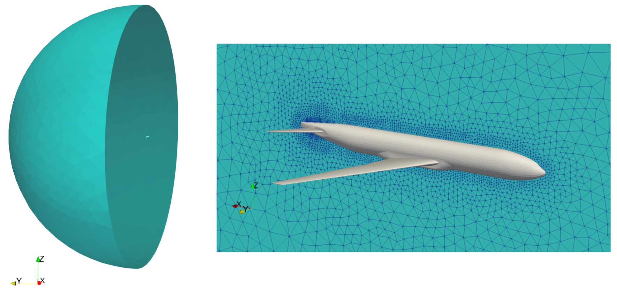
Figure 1: CRM: hemispherical computational fluid domain with a symmetry plane (left); and partial view of its discretization by an inviscid, unstructured, body-fitted mesh (right).

The parametric von Mises stress field is computed using the FE structural representation of half of the flexible CRM configuration shown in Figure 2, which has 58,888 degrees of freedom (dofs). In this representation, the FE structural modeling of the wing is that described in ^Kenway2014c. The other components of the FE structural representation shown in Figure 2 were developed by the authors and incorporated in the final FE structural model to facilitate two-way coupled aeroelastic computations.

The flutter avoidance constraint is the most CPU intensive constraint in the formulation of the MDAO problem (46). It is approximated using a database of linear FSI PROMs.

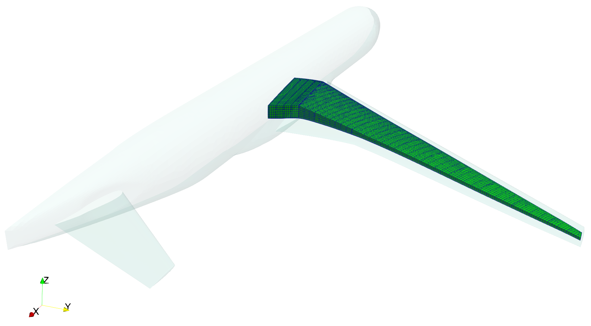
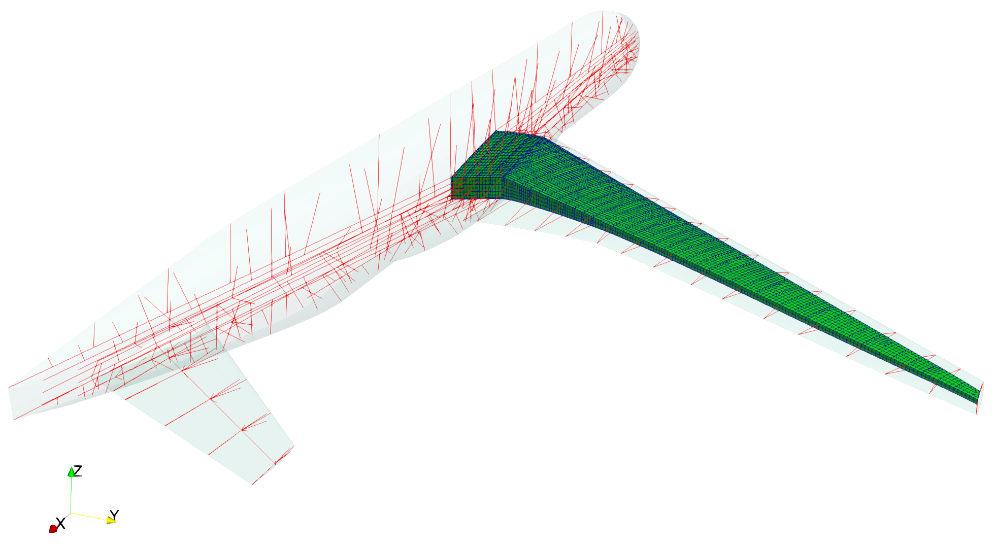
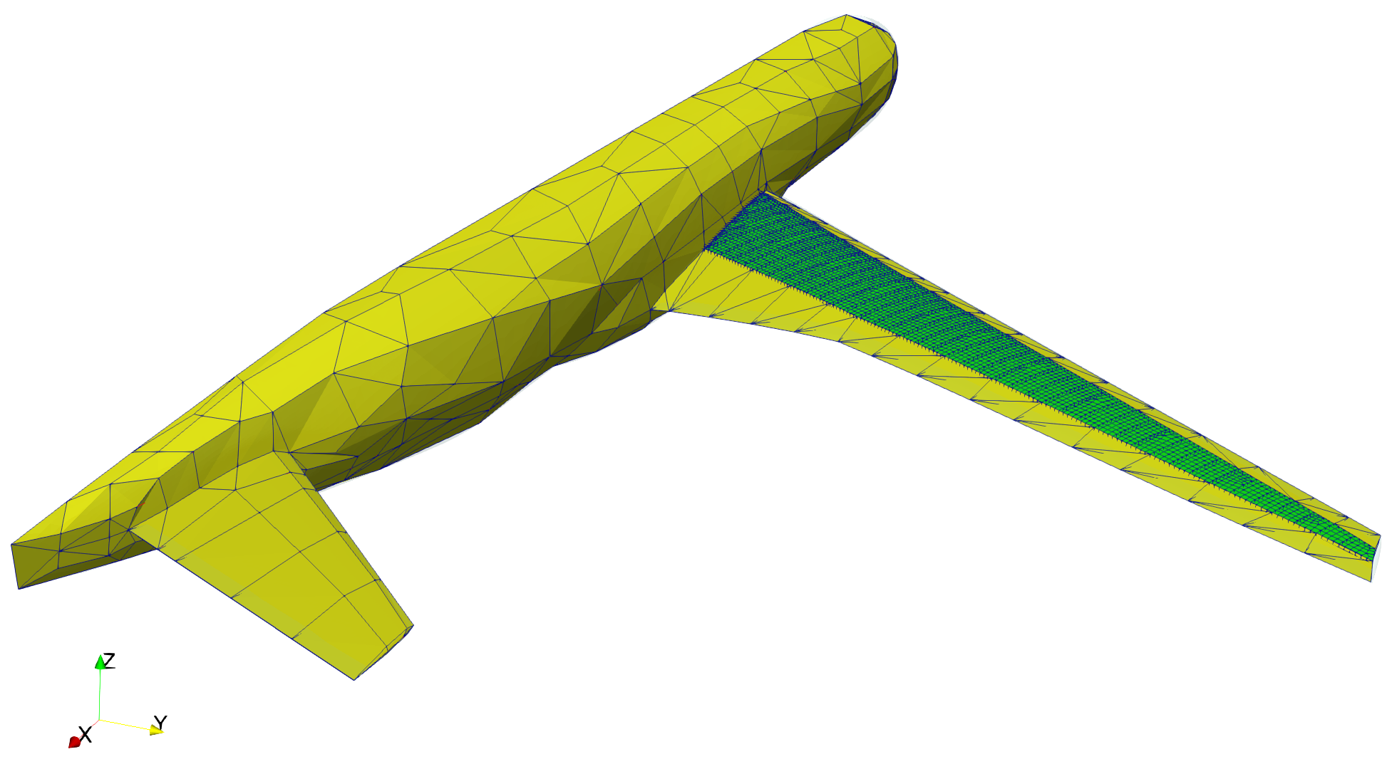
Figure 2: CRM – FE structural respresentations of: wing (top); fuselage and control surfaces (middle); and skin (bottom).

The six design optimization parameters stored in $\boldsymbol{\mu}$ are organized in two groups: three optimization parameters $\{\boldsymbol{\mu}[1],\boldsymbol{\mu}[2],\boldsymbol{\mu}[3]\}$ that are shape design parameters, and three optimization parameters $\{\boldsymbol{\mu}[4],\boldsymbol{\mu}[5],\boldsymbol{\mu}[6]\}$ that are structural design parameters.

The three shape design parameters are chosen as follows: $\boldsymbol{\mu}[1]$ and $\boldsymbol{\mu}[2]$ to control the dihedral angle of the wing; and $\boldsymbol{\mu}[3]$ to control its sweep angle. All shape changes dictated by the optimization procedures are effected using the open-source 3D computer graphics software Blender ²¹. Figure 3 illustrates the concept of lattice-based deformations of Blender to effect shape changes ²², and Figure 4 graphically depicts the effects on the shape of the wing of the specified lower and upper bounds for the dihedral and sweep angles.

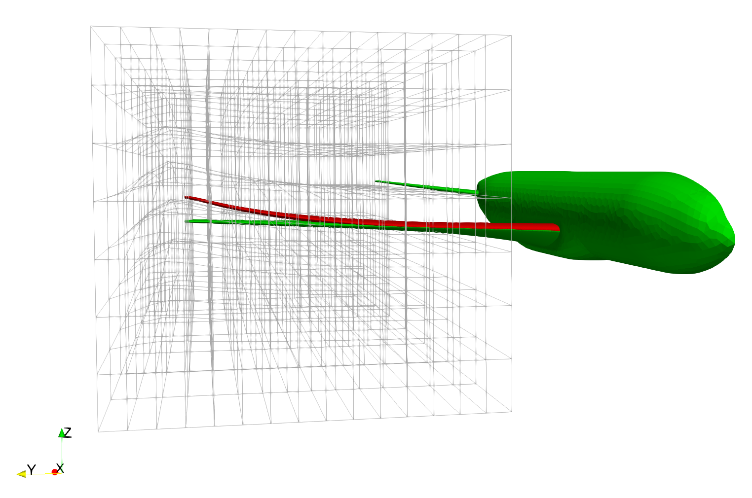
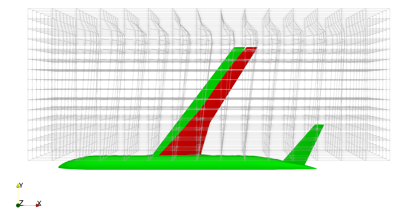
Figure 3: CRM – parameters controling: dihedral angle of the wing (left); and sweep angle of the wing (right).

Figure 4: CRM – wing shapes associated with: upper (green) and lower (red) bounds for the dihedral angle (left); and upper (green) and lower (red) bounds for the sweep angle (right).

The three structural design parameters are chosen as three thickness increments for three different groups of stiffeners (see Figure 5). Each increment is defined as a percentage of the initial thickness to which it is applied, and is constrained to have a magnitude less than 10% (box constraint).

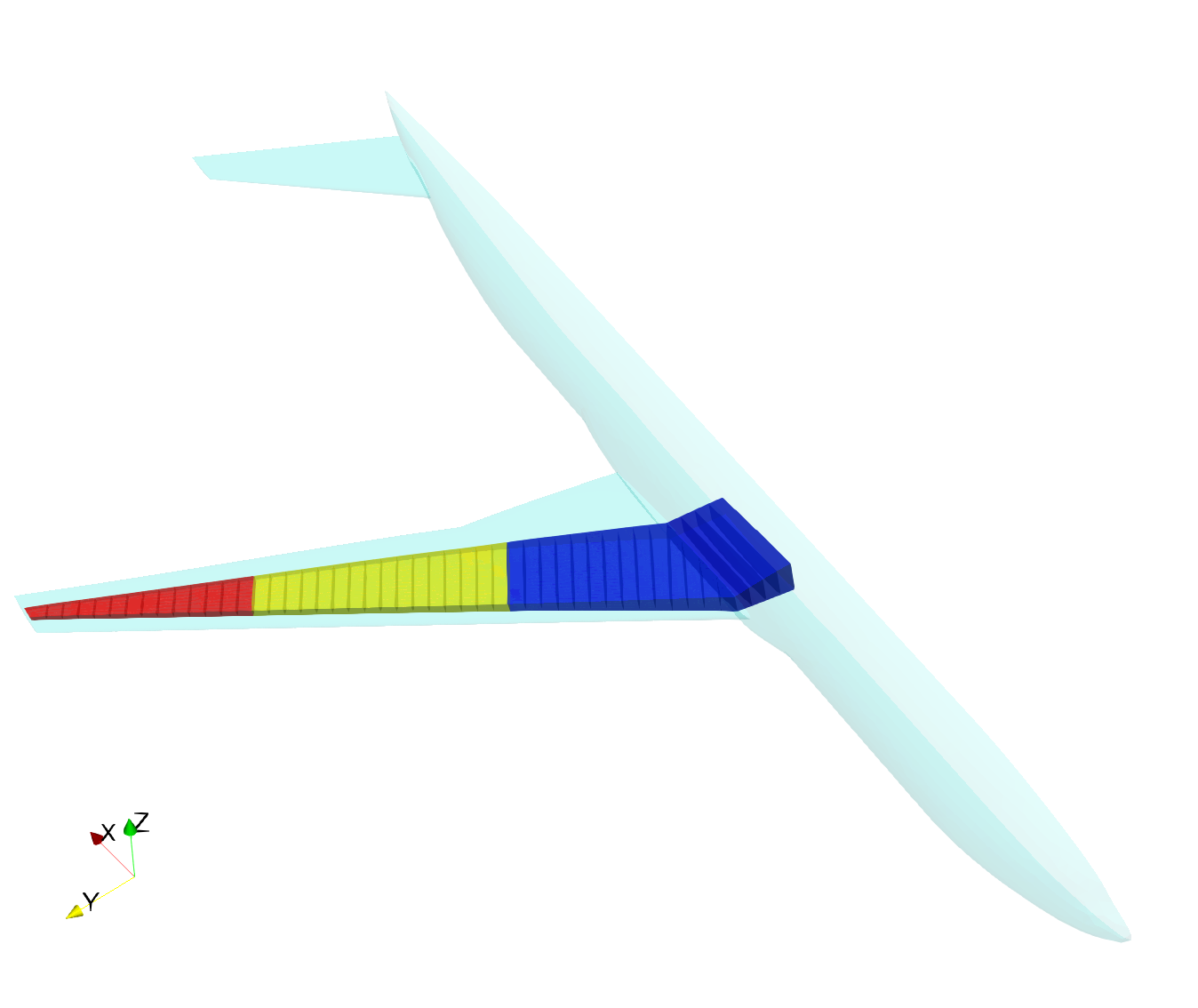
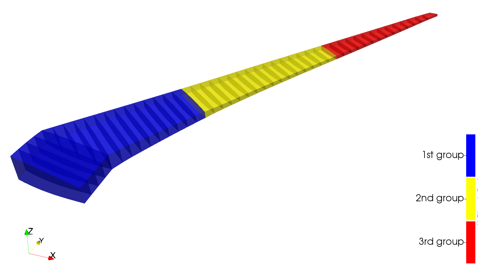
Figure 5: CRM – organization of the stiffeners of the wing in three different groups represented by three different colors.

4.2.1 Offline Construction of Databases of FSI PROMs

Three databases of FSI PROMs are built for the solution of the MDAO problem (46):

• ${\mathcal{D}B}_{1}$, which is constructed by directly sampling the design parameter space $\mathcal{D}$ using a greedy procedure similar to that described in Section 3.4, but applied directly to $\mathcal{D}$. The greedy procedure samples in this case $N_{\mathcal{D}B}=119$ feasible design parameter points.

• ${\mathcal{D}B}_{2}$, which is constructed by building first the lower-dimensional space of design parameter generalized coordinates ${\mathcal{G}}^{\,\text{cl}}$ using the classical AS method described in Section 3.1.1 and its associated empirical formula (12), then indirectly sampling $\mathcal{D}$ by directly sampling $\mathcal{G}$. In this case, the free parameters of formula (12) are chosen as $\alpha=10$ and $\beta=6$, which yields $N_{\mathbf{S}}=47$. Hence, 47 gradients of the objective function are computed at 47 feasible parameter points that are randomly sampled in $\mathcal{D}$ using the LHS method. The computation of each gradient consumes 0.3 hour wall-clock time on a Linux cluster with 240 processors. Next, the computed snapshots are compressed into a ROB $\mathbf{V}_{\mu}$ of dimension $n_{\mathcal{G}}^{\text{cl}}=3$ (see below).

• ${\mathcal{D}B}_{3}$, which is constructed by building first ${\mathcal{G}}^{\,\text{al}}$ using the alternative AS method described in Section 3.1.2, then indirectly sampling $\mathcal{D}$ by directly sampling $\mathcal{G}$, using the greedy procedure described in Section 3.4. In this case, the snapshots of the form $\Delta\boldsymbol{\mu}$ are adaptively computed by solving the auxiliary optimization problem

  $$\underset{\boldsymbol{\mu}\,\in\,\mathcal{D}\,\subset\,\mathbb{R}^{6}}{\text{maximize}} \frac{L(\boldsymbol{\mu})}{D(\boldsymbol{\mu})}$$ (47)

  subject to $$\sigma_{\text{VM}}(\boldsymbol{\mu})\leq\sigma_{\text{ub}}$$

  $$\boldsymbol{\mu}_{\text{lb}}\leq\boldsymbol{\mu}\leq\boldsymbol{\mu}_{\text{ub}}$$

  which is obtained by removing from the MDAO problem (46) the CPU intensive FSI constraint. This auxiliary problem is solved in 16 iterations using the sequential least-squares programming method SLSQP, which uses the Han-Powell quasi-Newton method with a BFGS update and an $L_{1}$ test function in the step-length algorithm. Hence, the solution of the optimization problem (47) generates 17 snapshots. The computation of each of the snapshots consumes about 0.34 hour wall-clock time – roughly the same amount of time as the computation of a gradient snapshot in the classical AS method – on the same Linux cluster. Next, the snapshots are compressed into a ROB $\mathbf{V}_{\mu}$ of dimension $n_{\mathcal{G}}^{\text{al}}=3$ (see below).

Figure 6 plots the distributions of the singular values of both matrices $\mathbf{S}$ (11) and $\mathbb{S}$ (15). For the snapshot matrix $\mathbf{S}$ associated with the classical AS method, there is no clear cutoff singular value for constructing a ROB $\mathbf{V}_{\mu}$, as the singular values are shown to continuously decay. For the snapshot matrix $\mathbb{S}$ associated with the alternative AS method however, Figure 6-right shows that the last three singular values are much smaller than the first three ones. This suggests constructing a ROB $\mathbf{V}_{\mu}$ as the set of the first three columns of the matrix $\mathbf{U}$ arising from the SVD of $\mathbb{S}$ – that is, constructing a ROB $\mathbf{V}_{\mu}$ of dimension $n_{\mathcal{G}}^{\text{al}}=3$. Hence, the dimension of $\mathbf{S}$ is also set to $n_{\mathcal{G}}^{\text{cl}}=3$, in order to enable various meaningful performance comparisons.

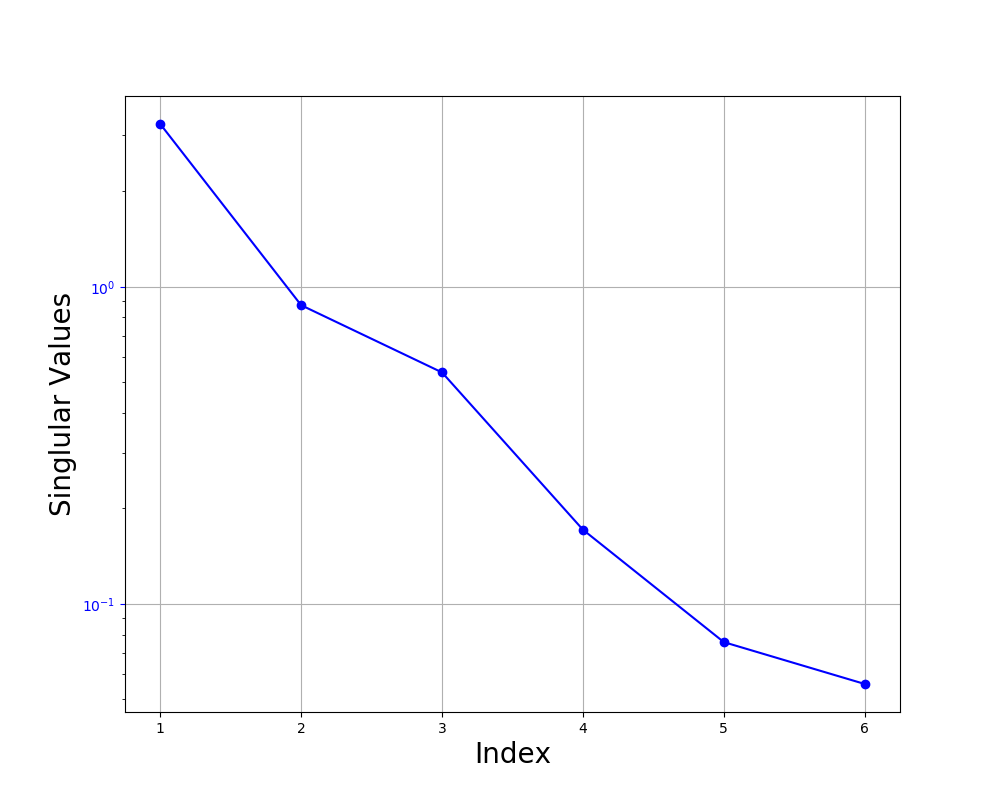
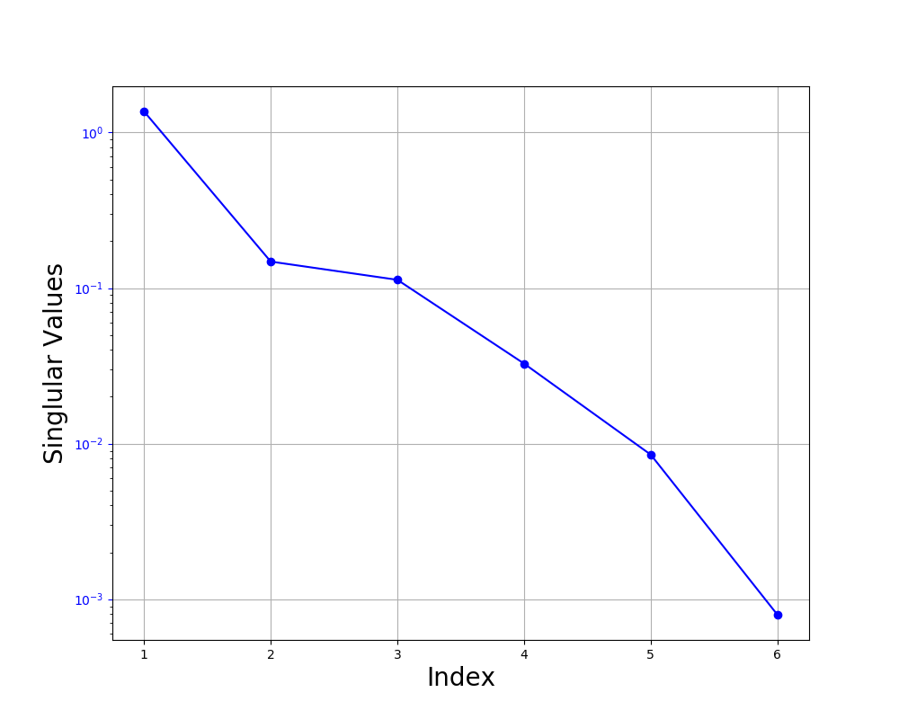
Figure 6: Singular values of: the snapshot matrix $\mathbf{S}$ computed using the classical AS method (left); and the counterpart matrix $\mathbb{S}$ computed using the alternative AS method (right).

The concept of indirectly sampling $\mathcal{D}$ by directly sampling the lower-dimensional space $\mathcal{G}$ using the feasible AS algorithm (Algorithm 3) is illustrated in Figure 7, for the case of the problem considered herein and ${\mathcal{D}B}_{3}$. First, a set of 1,000 preliminary points is generated in ${\mathcal{G}}^{\,\text{al}}$ using a uniform tensor product in this parameter space. Next, Algorithm 3 is applied to select among these points a set $\Xi_{r}$ of 323 feasible candidate points (see Figure 7-left), and determine the associated set of feasible points $\Xi\in\mathcal{D}$ (see Figure 7–right). Then, the greedy algorithm described in Section 3.4 is directly applied to $\Xi_{r}$ – and indirectly to $\Xi$ – to perform the final parameter sampling and adaptively construct the database of FSI PROMs ${\mathcal{D}B}_{3}$. Note that the feasible parameter points in $\Xi$ are not uniformly spread in $\mathcal{D}$, but only in some regions of this design parameter space that depend on the ROB $\mathbf{V}_{\mu}$ (see Figure 7). The plot in the $i$-th diagonal of Figure 7-left shows the distribution of the $i$-th component $\boldsymbol{\mu}_{r}[i]$ of the candidate parameter points in $\Xi_{r}$. Its counterpart in Figure 7-right shows the distribution of the $i$-th component $\boldsymbol{\mu}[i]$ of the corresponding candidate parameter points in $\Xi$. The plot in the $(i,j)$ off-diagonal of Figure 7-right shows the distribution of the contribution of the $j$-th generalized coordinate $\boldsymbol{\mu}_{r}[j]$ to the $i$-th component $\boldsymbol{\mu}[i]$ of the candidate parameter point $\boldsymbol{\mu}$ in $\Xi$.

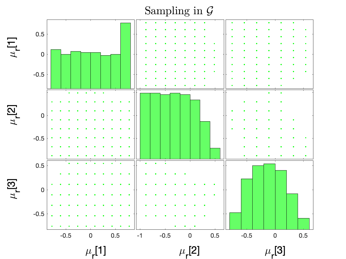
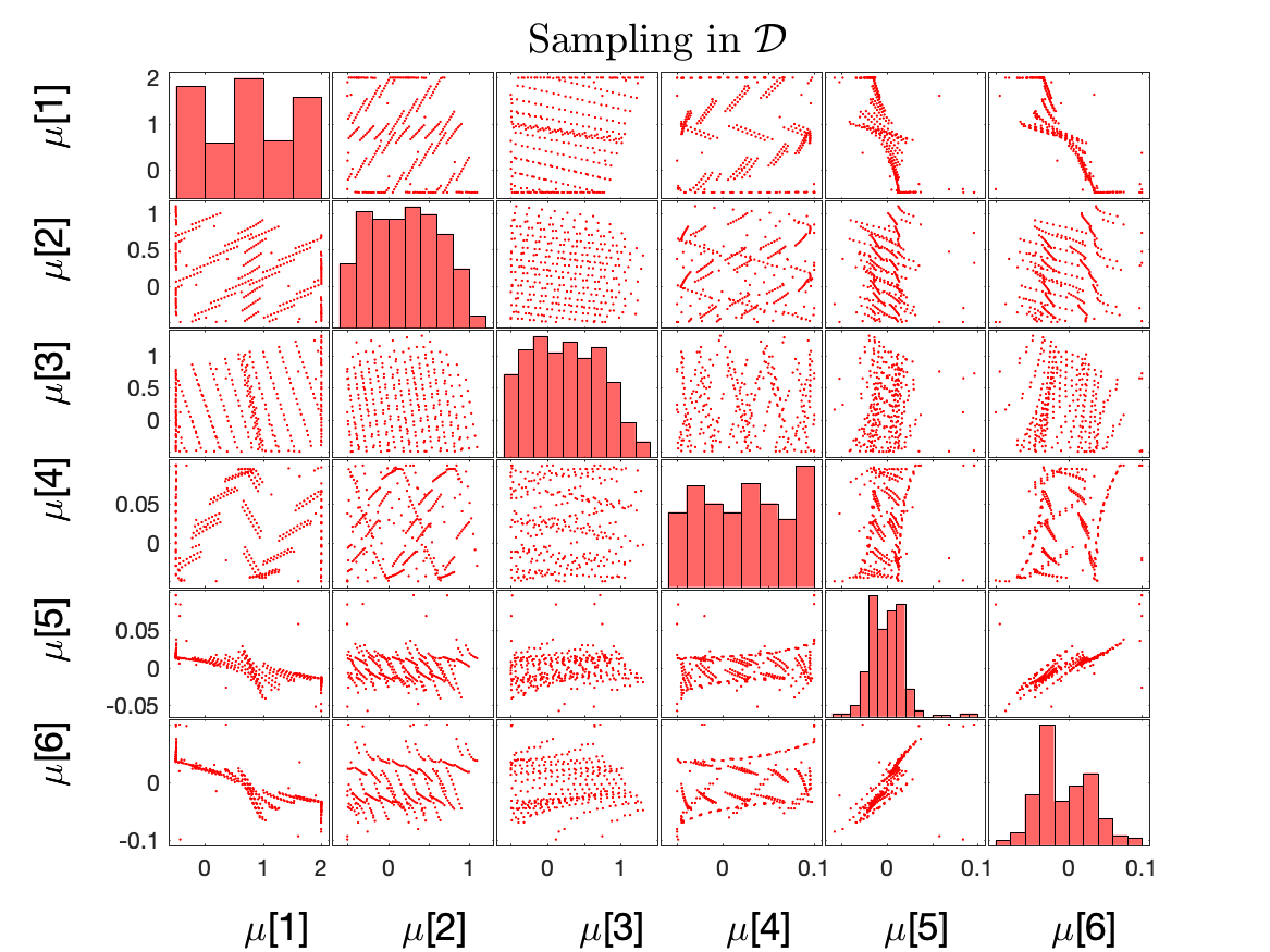
Figure 7: Set $\Xi_{r}\in{\mathcal{G}}^{\,\text{al}}$ containing 323 feasible candidate points determined by the feasible AS algorithm as well as the alternative approach for constructing an AS (left), and associated set $\Xi\in\mathcal{D}$ containing the same number of feasible candidate points (right).

In each constructed database, each pre-computed linear FSI PROM is built as described in Section 3.2, with $n_{f}=100$ and $n_{s}=6$. Hence, each pre-computed linear FSI PROM has the dimension $n_{q}=n_{f}+2n_{s}=112$.

Table (3) reports on the performance of the offline phase for problem (46) of the computational framework for MDAO described in this paper, depending on whether an AS is used or not, and which method is chosen to construct it. The following observations are noteworthy:

• Even when using the same greedy procedure equipped with the same convergence tolerance, the database of linear FSI PROMs ${\mathcal{D}B}_{3}$ ends up being less populated than ${\mathcal{D}B}_{1}$. This is because in this case, ${\mathcal{D}B}_{3}$ is constructed to be as accurate as ${\mathcal{D}B}_{1}$, but in a smaller parameter space. Similarly, ${\mathcal{D}B}_{2}$ is constructed to be as accurate as ${\mathcal{D}B}_{1}$ – albeit using a different construction procedure – but in a smaller parameter space.

• The computational cost of the greedy procedure is roughly proportional to the number of sampled parameter points, which itself appears to be proportional to the dimension of the sampled parameter space.

• Furthermore, even after accounting for the computational overhead associated with constructing a representative basis $\mathbf{V}_{\mu}$, an AS speeds up the construction of a database of PROMs. It remains to asses next however, the performance of each database constructed using an AS relative to the performance of ${\mathcal{D}B}_{1}$, which is built without an AS.

Table 3: CRM: performance results for the offline phase

Method	$N_{\mathcal{D}}$	$N_{\mathbf{S}}$ or $N_{\mathbb{S}}$	Wall-clock time	$N_{\mathcal{D}B}$	Wall-clock time	Wall-clock time	Speed-up
			computing $\mathbf{V}_{\mu}$		greedy procedure	total offline	relative to no AS
w/o AS	6	N.A.	N.A.	119	120.87 hrs	120.87 hrs	N.A.
Classical AS	3	47	14.06 hrs	61	61.95 hrs	76.01 hrs	1.59
Alternative AS	3	17	5.83 hrs	62	62.97 hrs	68.80 hrs	1.76

4.2.2 Online Prediction and Aeroelastic Optimization

Figure 8 and Figure 9 display the convergence histories of the objective function and constraints of the MDAO problem (46), respectively. They highlight that, at least for this CRM MDAO problem, the classical AS method leads to an ineffective optimization strategy. Indeed, both figures reveal that in the case of the classical AS method, the PROM-based computational framework described in this paper fails to improve the objective function beyond its initial value. On the other hand, the same computational framework equipped with the alternative AS method leads to almost the same optimal objective function and constraints as its counterpart framework equipped with direct sampling of the entire design parameter space, and in almost the same number of iterations. In particular, note that during the first few iterations, the alternative AS method leads to the same values of the optimized objective function and constraints as directly sampling the full space ${\mathcal{D}}$. This is because during the first few iterations, the flutter constraint is inactive, the auxiliary MDAO problem (47) is in this case identical to the original MDAO problem (46), and thereore the basis $\mathbf{V}_{\mu}$ based on the snapshot matrix $\mathbb{S}$ (15) is optimal.

Table 4) shows the optimal solution of the MDAO problem (46) obtained using the three different PROM databases ${\mathcal{D}B}_{1}$, ${\mathcal{D}B}_{2}$, and ${\mathcal{D}B}_{3}$. The reader can observe that the optimal solution obtained using the PROM database ${\mathcal{D}B}_{2}$ – that is, the classical AS method for sampling – is far from its counterpart obtained using the PROM database ${\mathcal{D}B}_{1}$ – that is, by directly sampling the design parameter space $\mathcal{D}$. On the other hand, the local optimal solution obtained using the PROM database ${\mathcal{D}B}_{3}$ – that is, the aternative AS method for sampling – is relatively close to its counterpart obtained using the database of linear FSI PROMs ${\mathcal{D}B}_{1}$.

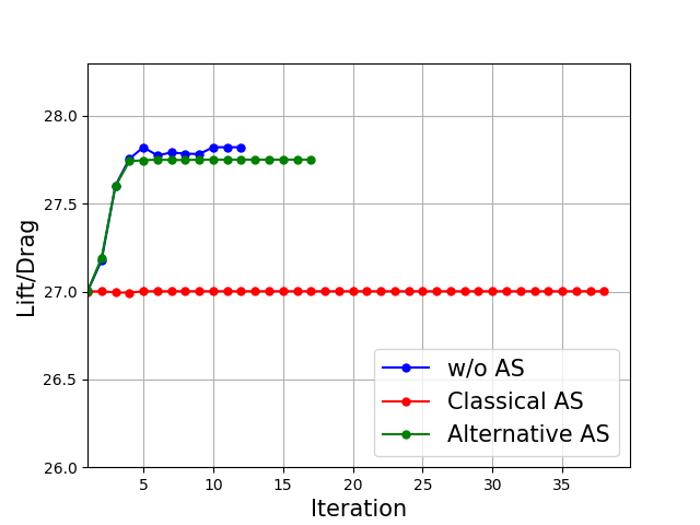
Figure 8: CRM: convergence histories of the objective function.

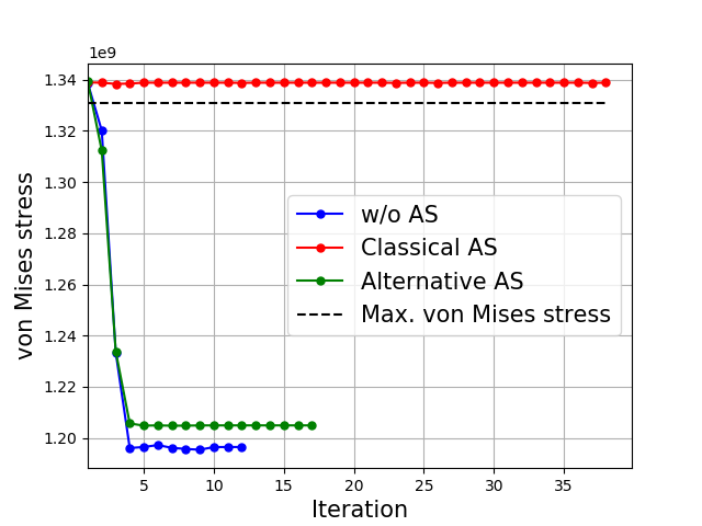
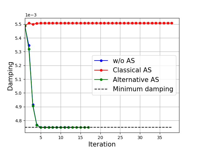
Figure 9: CRM: convergence histories of the constraints.

Table 4: CRM: locally optimal computed solutions

	$\boldsymbol{\mu}[1]$	$\boldsymbol{\mu}[2]$	$\boldsymbol{\mu}[3]$	$\boldsymbol{\mu}[4]$	$\boldsymbol{\mu}[5]$	$\boldsymbol{\mu}[6]$
Initial configuration	0.0	0.0	0.0	0.0	0.0	0.0
Specified lower bound	-0.5	-0.5	-0.5	-0.05	-0.1	-0.1
Specified upper bound	2.0	2.0	2.0	0.1	0.1	0.1
Optimal configuration using ${\mathcal{D}B}_{1}$	-0.50	-0.16	1.47	0.07	0.05	0.06
Optimal configuration using ${\mathcal{D}B}_{2}$	$1.6\times 10^{-4}$	$-1.1\times 10^{-5}$	$-2.3\times 10^{-3}$	$-4.9\times 10^{-2}$	$-3.0\times 10^{-3}$	$5.0\times 10^{-3}$
Optimal configuration using ${\mathcal{D}B}_{3}$	-0.32	-0.15	1.35	0.10	0.05	0.08

In summary, for this MDAO problem with six design optimization parmeters only, the alternative subspace method speeds up the offline computations by almost a factor two, while leading to a reasonably close local optimum solution.

Next, another MDAO problem with a larger number of design optimization parameters is considered.

4.3 Aeroelastic Design Optimization of a Parametric ARW-2 Configuration

Next, the following fifteenth-dimensional MDAO problem for NASA’s ARW-2, whose geometrical and material descriptions are summarized in Table 5, is considered

$$\underset{\boldsymbol{\mu}~{}\in~{}\mathcal{D}~{}\subset~{}\mathbb{R}^{15}}{\text{maximize}} \frac{L(\boldsymbol{\mu})}{D(\boldsymbol{\mu})}$$ (48)

subject to $$W(\boldsymbol{\mu})\leq W_{\text{ub}}$$

$$\sigma_{\text{VM}}(\boldsymbol{\mu})\leq\sigma_{\text{ub}}$$

$$\boldsymbol{\mu}_{\text{lb}}\leq\boldsymbol{\mu}\leq\boldsymbol{\mu}_{\text{ub}}$$

$$\boldsymbol{\zeta}(\boldsymbol{\mu})\geq\textbf{1}\zeta_{\text{lb}}$$

where:

• $L(\boldsymbol{\mu})$ and $D(\boldsymbol{\mu})$ denote as before the parametric lift and drag, respectively, associated here with the following flight conditions:

  • Level flight at the altitude of $h=4,000$ ft, where the free-stream pressure and density are $P_{\infty}=12.7\hskip 3.0pt\text{lb/in}^{2}$ and $\rho_{\infty}=1.0193\times 10^{-7}\hskip 3.0pt\text{lb}\cdot\text{s}^{2}/\text{in}^{4}$, respectively.

  • Free-stream Mach number $M_{\infty}=0.8$, angle of attack AoA $=0^{\circ}$, and angle of sideslip AoS $=0^{\circ}$.

• $W(\boldsymbol{\mu})$ denotes the parametric weight of the ARW-2, and $W_{\text{ub}}$ is its upper bound set to $W_{\text{ub}}=400$ lbs.

• The upper bound for the parametric von Mises stress field is set to $\sigma_{\text{ub}}=2.3\times 10^{4}$ psi.

• $\textbf{1}\in\mathbb{R}^{15}$ and ${\bf 0}\in\mathbb{R}^{15}$ are vectors of ones and zeros, respectively, and the lower bound coefficient $\zeta_{\text{lb}}$ is set to $\zeta_{\text{lb}}=3.9\times 10^{-4}$.

Table 5: Geometrical and material descriptions of the ARW-2.

	Item	Value
Geometry
Wing	span	104.9 in
	root chord	40.2 in
	tip chord	12.5 in
Materials
Skin, except flaps
(various composite materials)
Stiffeners (aluminum)	E	$1.03\times 10^{7}$ psi
	$\rho$	$2.6\times 10^{-4}$ $lbf\cdot s^{2}/\text{in}^{4}$
	$\nu$	0.32

The computational fluid domain is chosen to be a cylinder surrounding the wing. It is discretized by a 3D, unstructured, body-fitted CFD mesh with $63,484$ grid points (see Figure 10). As in the previous example, the parametric lift and drag are obtained by postprocessing the computed flow solution. The detailed FE structural model of the wing includes representations of the spars, ribs, hinges, and control surfaces (see Figure 11). It contains a total of $2,556$ dofs. The parametric weight and von Mises stress field are computed using this FE representation. The flutter avoidance constraint, which is also in this case the most CPU intensive constraint, is approximated using a database of linear FSI PROMs.

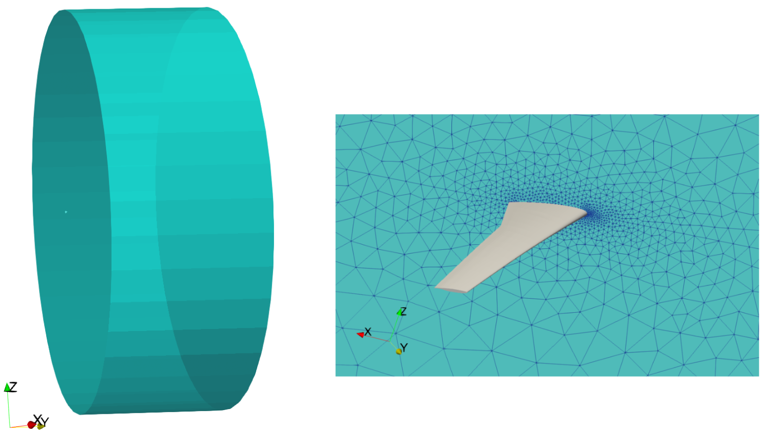
Figure 10: ARW-2: cylindrical computational fluid domain with a symmetry plane (left); and discretization by an inviscid, unstructured, body-fitted mesh (right).

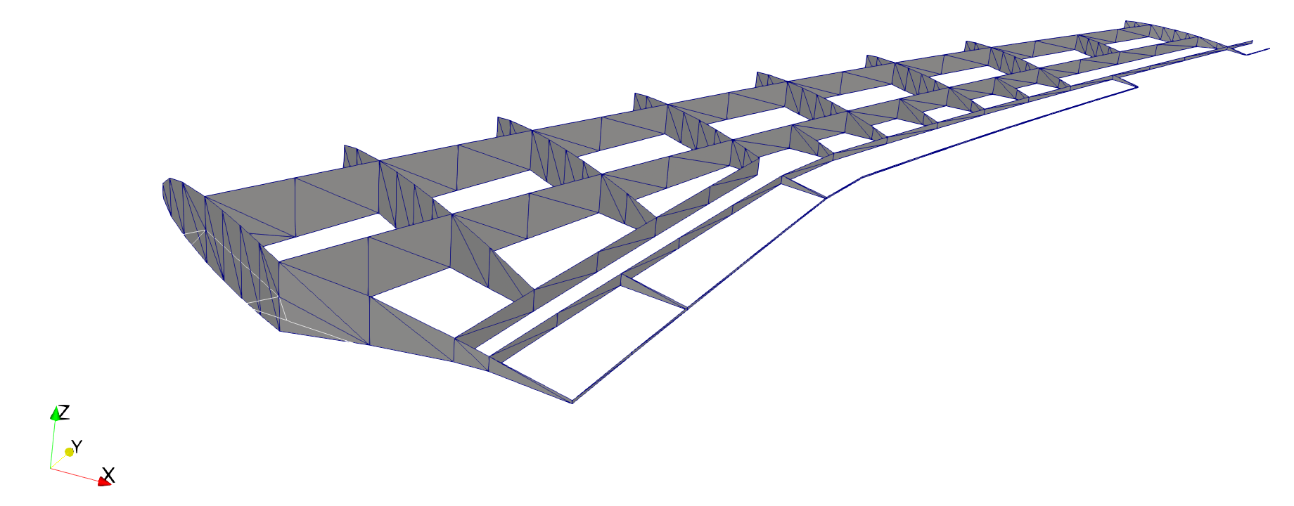
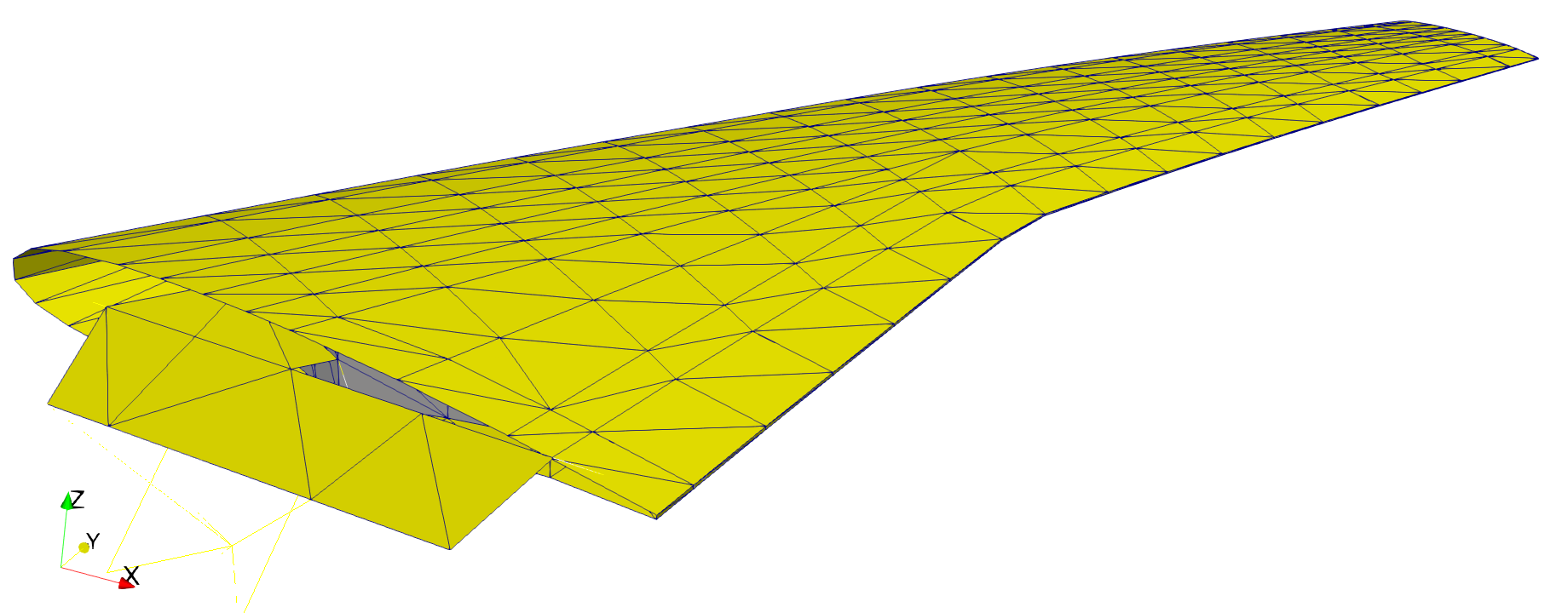
Figure 11: ARW-2 – FE respresentations of: spars and ribs (top); and skin (bottom).

The 15 design optimization parameters stored in $\boldsymbol{\mu}$ are organized in two groups: eight shape design parameters $\{\boldsymbol{\mu}[1],\boldsymbol{\mu}[2],\boldsymbol{\mu}[3],\boldsymbol{\mu}[4],\boldsymbol{\mu}[5],\boldsymbol{\mu}[6],\boldsymbol{\mu}[7],\boldsymbol{\mu}[8]\}$, and seven structural design parameters $\{\boldsymbol{\mu}[9],\boldsymbol{\mu}[10],\boldsymbol{\mu}[11],\boldsymbol{\mu}[12],\boldsymbol{\mu}[13],\boldsymbol{\mu}[14],\boldsymbol{\mu}[15]\}$. The eight shape design parameters are chosen as follows: $\mu^{1}$ acts on the stretching of the wingspan; $\mu^{2}$ and $\mu^{3}$ modify the twist angle of the wing; $\mu^{4}$ and $\mu^{5}$ modify its dihedral angle; $\mu^{6}$ acts on its backsweep angle; $\mu^{7}$ modifies the wingspan taper; and $\mu^{8}$ controls the chord stretching of the wing.

Again, all shape changes dictated by the optimization procedures are effected using Blender ²¹.

Figures 12–14 graphically depict the effects on the shape of the ARW-2 of the specified lower and upper bounds for the wingspan stretching, twist angle, dihedral angle, backsweep angle, wingspan taper, and chord stretching of this wing.

The seven structural design parameters are chosen as seven thickness increments for seven different groups of stiffeners (see Figure 15). As before, each increment is defined as a percentage of the initial thickness to which it is applied, and is constrained to have a magnitude less than 10% (box constraint).

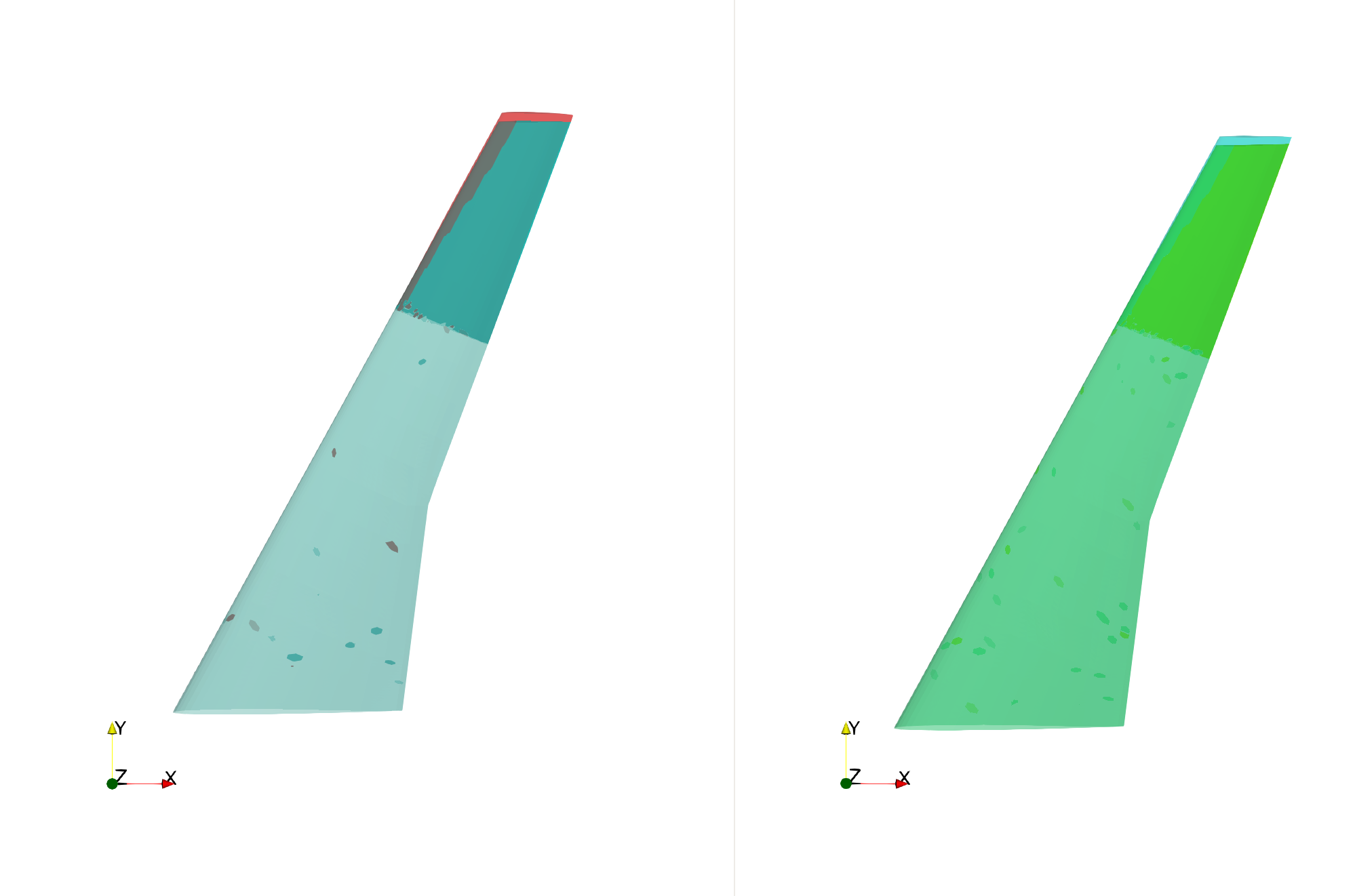
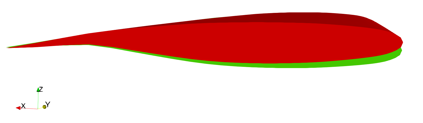
Figure 12: ARW-2 – wing shapes associated with: upper (green) and lower (red) bounds on the wingspan stretching (top); and upper (green) and lower (red) bounds on the twist angle (bottom).

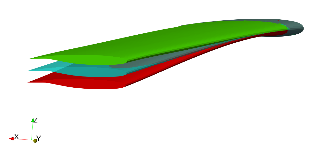
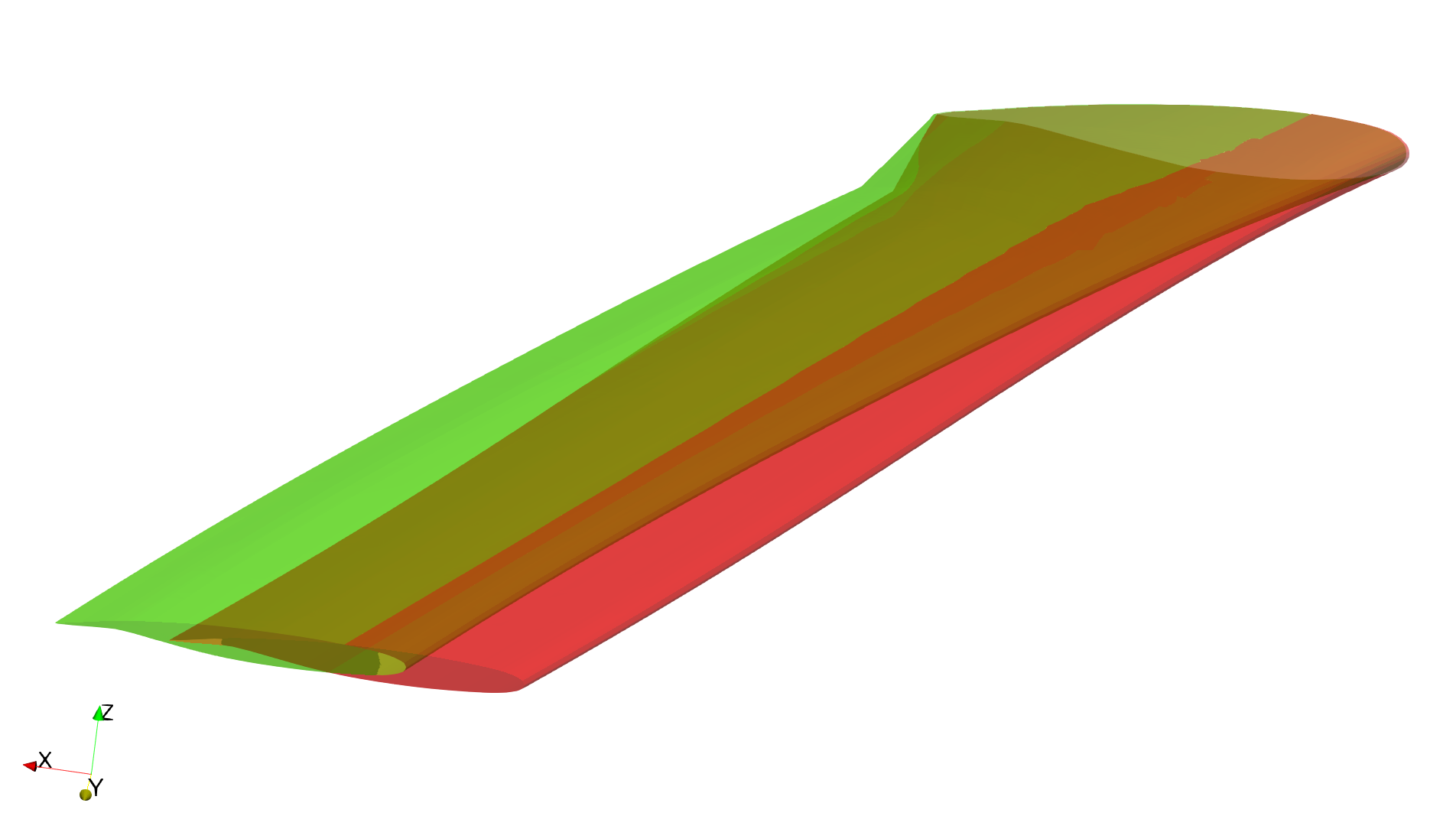
Figure 13: ARW-2 – wing shapes associated with: upper (green) and lower (red) bounds on the dihedral angle (top); and upper (green) and lower (red) bounds on the sweep angle (bottom).

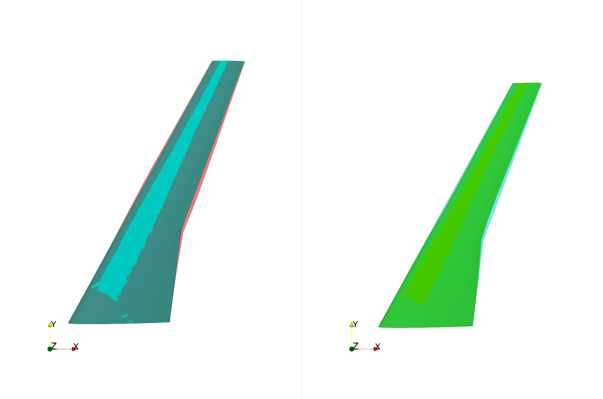
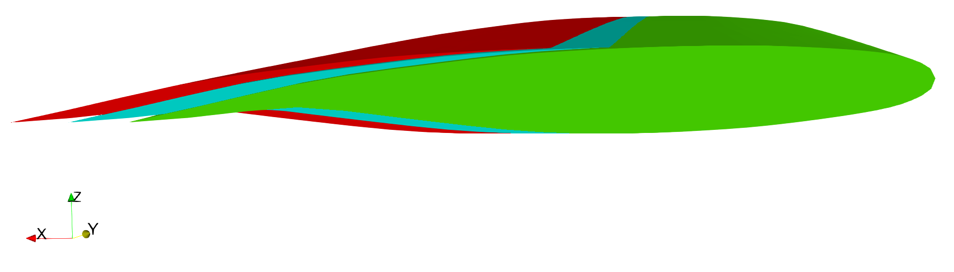
Figure 14: ARW-2 – wing shapes associated with: upper (green) and lower (red) bounds on the wingspan taper (top); and upper (green) and lower (red) bounds on the chord stretching (bottom).

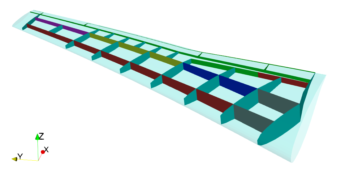
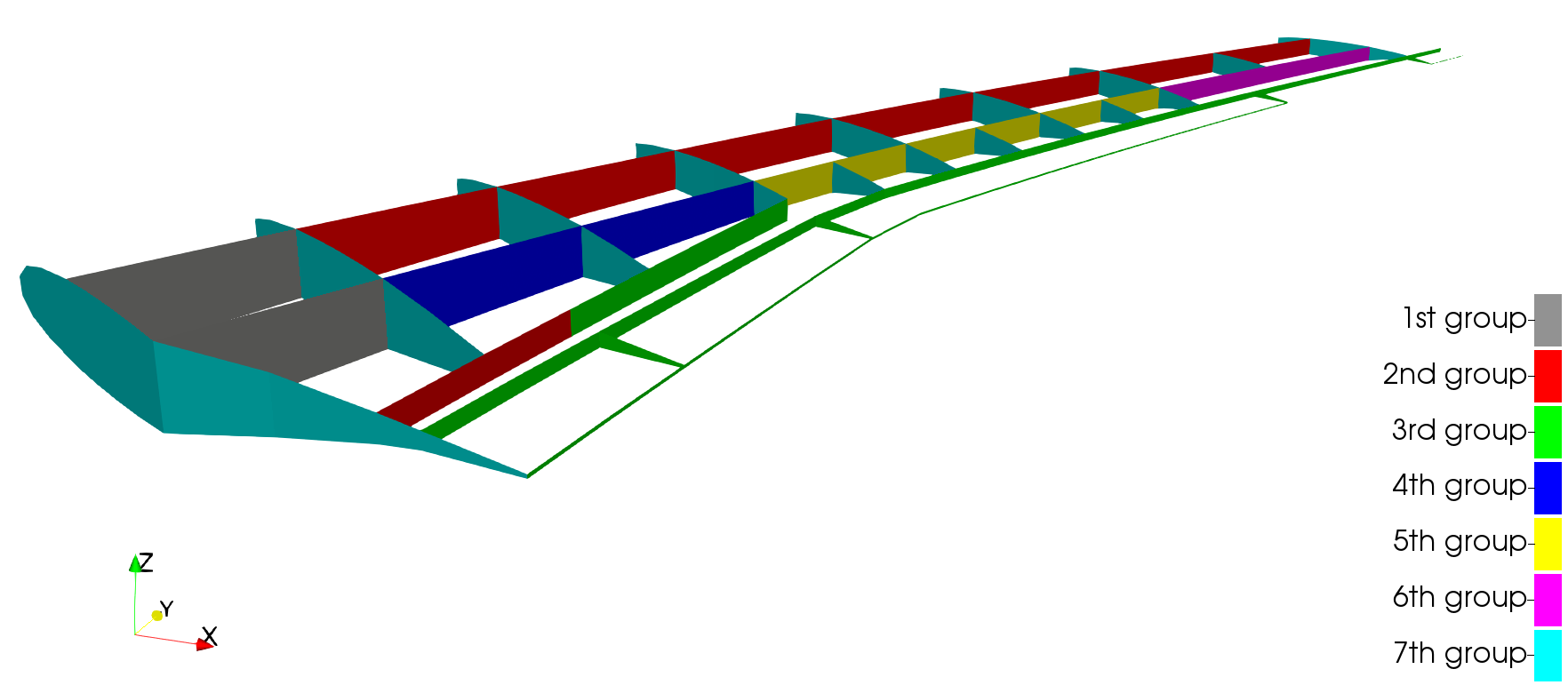
Figure 15: ARW-2 – organization of the stiffeners of the wing in seven different groups represented by seven different colors.

4.3.1 Offline Database Construction

Given that for the MDAO problem (46) the PROM-based computational framework equipped with the classical AS method for indirectly sampling the design parameter space failed to improve the objective function beyond its initial value, only two databases of FSI PROMs are considered here for the solution of the MDAO problem (48):

• ${\mathcal{D}B}_{1}$, which is constructed as for the MDAO problem (46) (see Section 4.2.1). However, the greedy procedure samples in this case $N_{\mathcal{D}B}=415$ feasible design parameter points.

• ${\mathcal{D}B}_{3}$, which is constructed as for the MDAO problem (46) (see Section 4.2.1). In this case however, the snapshots of the form $\Delta\boldsymbol{\mu}$ are adaptively computed by solving the auxiliary optimization problem

  $$\underset{\boldsymbol{\mu}~{}\in~{}\mathcal{D}~{}\subset~{}\mathbb{R}^{15}}{\text{maximize}} \frac{L(\boldsymbol{\mu})}{D(\boldsymbol{\mu})}$$

  subject to $$W(\boldsymbol{\mu})\leq W_{\text{ub}}$$

  $$\sigma_{\text{VM}}(\boldsymbol{\mu})\leq\sigma_{\text{ub}}$$

  $$\boldsymbol{\mu}_{\text{lb}}\leq\boldsymbol{\mu}\leq\boldsymbol{\mu}_{\text{ub}}$$

  which is obtained by removing from the MDAO problem (48) the CPU intensive FSI constraint. This auxiliary problem is solved in 19 iterations using the SLSQP method. The 19 iterations generate 20 snapshots. The computation of each of the snapshots consumes about 5.3 minutes wall-clock time on a Linux cluster with 36 processors. Next, the snapshots are compressed into a ROB $\mathbf{V}_{\mu}$ of dimension $n_{\mathcal{G}}^{\text{al}}=7$ (see below).

Figure 16 plots the distributions of the singular values of the snapshot matrix $\mathbb{S}$ (15). It shows that the last eight singular values of this matrix are much smaller than the first seven ones. This suggests constructing a ROB $\mathbf{V}_{\mu}$ as the set of the first seven columns of the matrix $\mathbf{U}$ arising from the SVD of $\mathbb{S}$ – that is, constructing a ROB $\mathbf{V}_{\mu}$ of dimension $n_{\mathcal{G}}^{\text{al}}=7$.

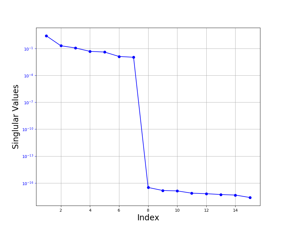
Figure 16: Singular values of the snapshot matrix $\mathbb{S}$ computed using the alternative AS method.

Figure 17 graphically depicts the characteristics of the sampling performed for constructing the database ${\mathcal{D}B}_{3}$. First, a set of 2,197 preliminary points is generated in ${\mathcal{G}}^{\,\text{al}}$ using a uniform tensor product in this parameter space. Next, Algorithm 3 is applied to select among these points a set $\Xi_{r}$ of 429 feasible candidate points (see Figure 17-left), and determine the associated set of feasible points $\Xi\in\mathcal{D}$ (see Figure 17–right). Then, the greedy algorithm described in Section 3.4 is directly applied to $\Xi_{r}$ – and indirectly to $\Xi$ – to perform the final parameter sampling and adaptively construct the database of FSI PROMs ${\mathcal{D}B}_{3}$. Each plot in the $i$-th diagonal of Figure 17-left, $i$-th diagonal of Figure 17-right, $(i,j)$ off-diagonal of Figure 17-left, and $(i,j)$ off-diagonal of Figure 17-right has the same meaning as in Figure 7 of Section 4.2.1.

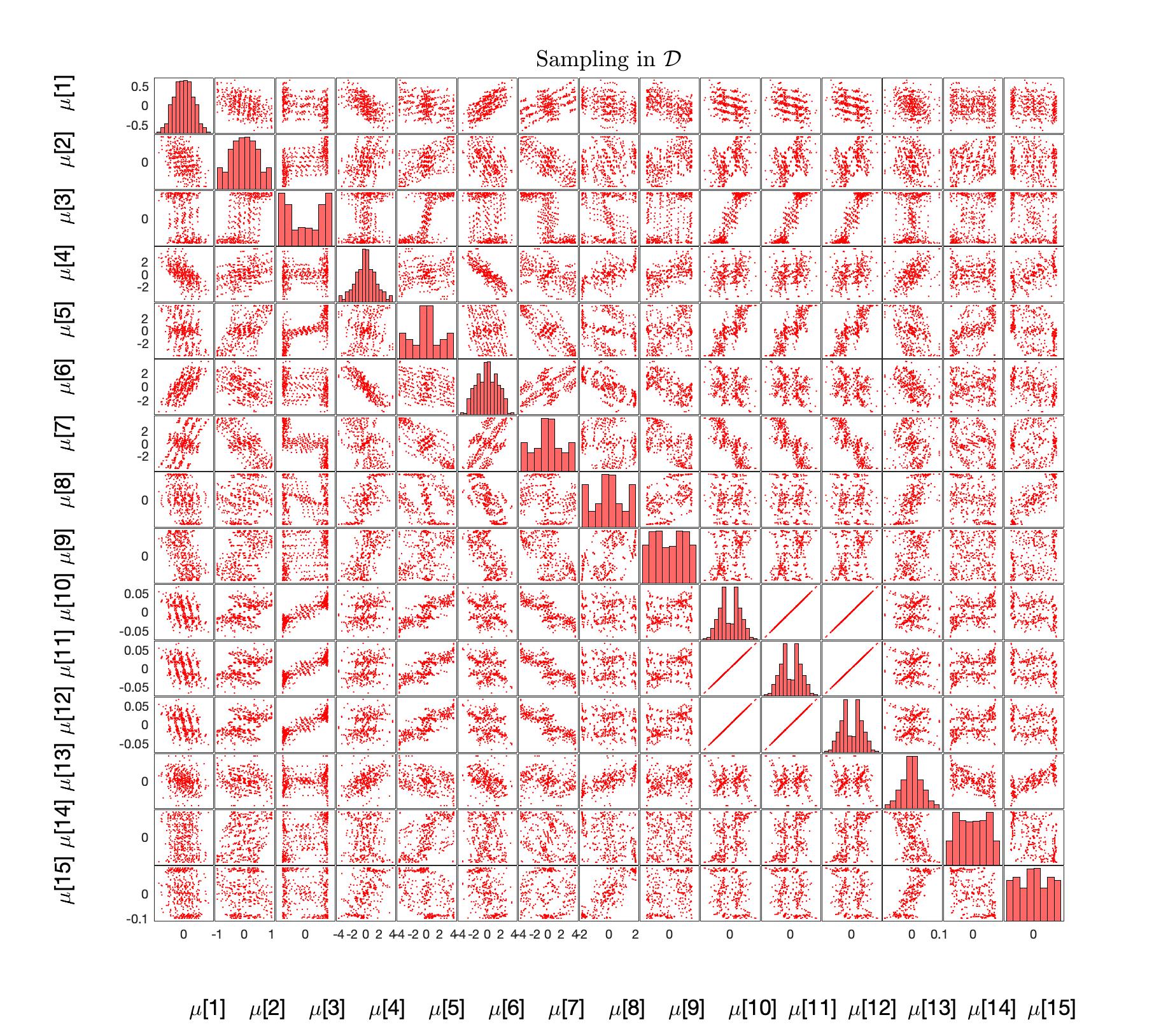
Figure 17: Set $\Xi_{r}\in{\mathcal{G}}^{\,\text{al}}$ containing 429 feasible candidate points determined by the feasible AS algorithm as well as the alternative approach for constructing an AS (left), and associated set $\Xi\in\mathcal{D}$ containing the same number of feasible candidate points (right).

In each constructed database, each pre-computed linear FSI PROM is built as described in Section 3.2, with $n_{f}=100$ and $n_{s}=6$. Hence, each pre-computed linear FSI PROM has the dimension $n_{q}=n_{f}+2n_{s}=112$.

Table 6 reports on the performance of the offline phase for problem (48) of the computational framework for MDAO described in this paper, depending on whether an AS is used or not. The same observations made in the previous example can also be made in this case. Additionally, the following comments are noteworthy:

• Whereas the advocates of the classical AS method recommend a number of samples $N_{\mathbf{S}}$ that grows logarithmically with the dimension of the design parameter space $N_{\mathcal{D}}$ (see (12)), the number of samples $N_{\mathbb{S}}$ obtained for both applications explored in this paper using the greedy procedure ${\mathcal{D}}$ does not obey the empirical formula (12).

• As $N_{\mathcal{D}}$ is increased, the speed-up relative to the case where no AS is used increases.

Table 6: ARW-2: performance results for the offline phase

Method	$N_{\mathcal{D}}$	$N_{\mathbb{S}}$	Wall-clock time	$N_{\mathcal{D}B}$	Wall-clock time	Wall-clock time	Speed-up
			computing $\mathbf{V}_{\mu}$		greedy procedure	total offline	relative to no AS
w/o AS	15	N.A.	N.A.	415	93.2 hrs	93.2 hrs	N.A.
Alternative AS	7	20	1.77 hrs	203	38.5 hrs	40.27 hrs	2.31

4.3.2 Online Prediction and Aeroelastic Optimization

Figure 18 and Figure 19 display the convergence histories of the objective function and constraints of the MDAO problem (48), respectively. They highlight that, as in the case of the CRM MDAO problem discussed in Section 4.2, the alternative AS method leads in this case to almost the same optimal objective function and constraints as the direct sampling of ${\mathcal{D}}$, and in roughly the same number of iterations. Again, the alternative AS method leads during the first few iterations to values of the optimized objective function and constraints that are similar to those obtained by directly sampling the full space ${\mathcal{D}}$. This, despite the fact that the flutter constraint is active early on during the iterations, and therefore the ROB $\mathbf{V}_{\mu}$ based on the snapshot matrix $\mathbb{S}$ (15) is by design sub-optimal; nevertheless, this ROB leads to good results.

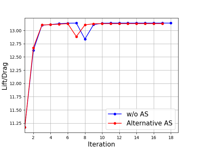
Figure 18: ARW-2: convergence histories of the objective function.

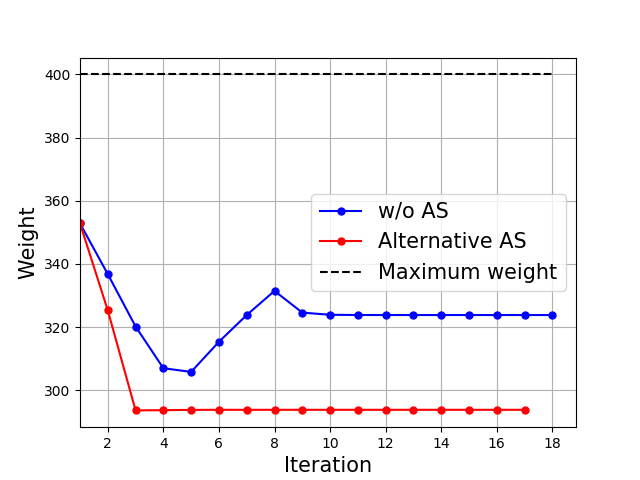
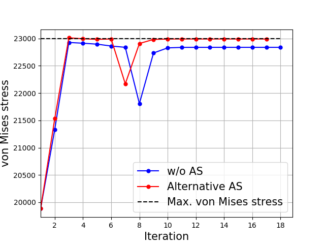
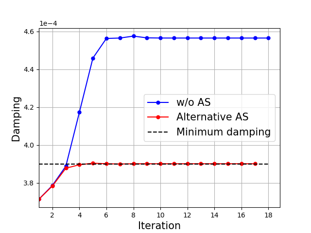
Figure 19: ARW-2: convergence histories of the constraints.

Table 7 compares the local optimal solutions of the MDAO problem (48) obtained using the two different PROM databases ${\mathcal{D}B}_{1}$ and ${\mathcal{D}B}_{3}$. The reader can observe that the optimal solution computed using the PROM database ${\mathcal{D}B}_{3}$ – that is, the aternative AS method for sampling – is sufficiently close to its counterpart computed using the database ${\mathcal{D}B}_{1}$. Since both databases of linear FSI PROMs lead to the same optimal value of the objective function (see Figure 18), the two solutions they deliver are different because they correspond to different local optimal points.

Table 7: ARW-2: locally optimal computed solutions

	$\boldsymbol{\mu}[1]$	$\boldsymbol{\mu}[2]$	$\boldsymbol{\mu}[3]$	$\boldsymbol{\mu}[4]$	$\boldsymbol{\mu}[5]$	$\boldsymbol{\mu}[6]$	$\boldsymbol{\mu}[7]$	$\boldsymbol{\mu}[8]$	$\boldsymbol{\mu}[9]$	$\boldsymbol{\mu}[10]$	$\boldsymbol{\mu}[11]$	$\boldsymbol{\mu}[12]$	$\boldsymbol{\mu}[13]$	$\boldsymbol{\mu}[14]$	$\boldsymbol{\mu}[15]$
Initial	0.0	0.0	0.0	0.0	0.0	0.0	0.0	0.0	0.0	0.0	0.0	0.0	0.0	0.0	0.0
Lower bound	-2	-1	-0.1	-4	-4	-4	-4	-2	-0.1	-0.1	-0.1	-0.1	-0.1	-0.1	-0.1
Upper bound	2	1	0.1	4	4	4	4	2	0.1	0.1	0.1	0.1	0.1	0.1	0.1
Optimal using ${\mathcal{D}B}_{1}$	1.32	0.95	-0.1	-0.98	0.14	-0.82	-0.66	-2.0	0.1	0.1	0.1	0.1	0.1	0.1	-0.05
Optimal using ${\mathcal{D}B}_{3}$	0.46	-0.09	-0.1	-0.16	-0.17	-0.31	-0.15	-0.22	0.1	0.1	0.1	0.1	0.1	0.1	-0.1

In summary, for this MDAO problem with fifteen design optimization parmeters, the alternative subspace method speeds up the offline computations by a factor bigger than two, while leading to a reasonably close local optimum solution.

5 Conclusions

A new take on the concept of an active subspace is presented for mitigating the curse of dimensionality associated with sampling a design parameter space for the purpose of model reduction in multidisciplinary analysis and optimization (MDAO). Instead of performing an empirical, a priori sampling of the gradient of the objective function of interest in order to construct a reduced-order basis for the optimization parameters, the alternative approach presented in this paper samples instead the solution trajectory of an economical version of the MDAO problem of interest in incremental form using an adaptive, greedy procedure guided by an efficient, residual-based error indicator. The new approach is intertwined with the concepts of projection-based model order reduction and a database of linear, projection-based reduced-order models (PROMs) equipped with interpolation on matrix manifolds, in order to construct a complete and efficient computational framework for MDAO problems incorporating a computationally intensive linearized fluid-structure interaction constraint. The framework is illustrated using two different MDAO problems associated with two different aeroelastic systems governed by flutter constraints: a flexible configuration of NASA’s Common Research Model; and NASA’s Aeroelastic Research Wing #2 (ARW-2). The obtained results demonstrate the superiority of the alternative approach described in this paper for constructing an active subspace over the classical one, and the feasibility of the proposed PROM-based computational framework for accelerating the solution of realistic MDAO problems.

References

- 1 Zahr MJ, Farhat C. Progressive construction of a parametric reduced-order model for PDE-constrained optimization. International Journal for Numerical Methods in Engineering 2015; 102(5): 1111–1135.
- 2 Amasallem D, Cortial J, Carlberg K, Farhat C. Towards real-time cfd-based aeroelastic computations using a database of reduced-order models. AIAA Journal 2010; 48: 2029–2037.
- 3 Amsallem D, Farhat C. An online method for interpolating linear parametric reduced-order models. SIAM Journal on Scientific Computing 2011; 33(5): 2169–2198.
- 4 Hesthaven JS, Stamm B, Zhang S. Efficient greedy algorithms for high-dimensional parameter spaces with applications to empirical interpolation and reduced basis methods∗. ESAIM: Mathematical Modelling and Numerical Analysis 2014; 48(1): 259–283.
- 5 Farhat C, Lesoinne M, Maman N. Mixed explicit/implicit time integration of coupled aeroelastic problems: three-field formulation, geometric conservation and distributed solution. International Journal for Numerical Methods in Fluids 1995; 21(10): 807–835.
- 6 Degand C, Farhat C. A three-dimensional torsional spring analogy method for unstructured dynamic meshes. Computers & structures 2002; 80(3-4): 305–316.
- 7 Jasak H, Tukovic Z. Automatic mesh motion for the unstructured finite volume method. Transactions of FAMENA 2006; 30(2): 1–20.
- 8 Farhat C, Lesoinne M, Le Tallec P. Load and motion transfer algorithms for fluid/structure interaction problems with non-matching discrete interfaces: Momentum and energy conservation, optimal discretization and application to aeroelasticity. Computer Methods in Applied Mechanics and Engineering 1998; 157(1-2): 95–114.
- 9 Lesoinne M, Sarkis M, Hetmaniuk U, Farhat C. A linearized method for the frequency analysis of three-dimensional fluid/structure interaction problems in all flow regimes. Computer Methods in Applied Mechanics and Engineering 2001; 190(24-25): 3121–3146.
- 10 Lukaczyk TW, Constantine P, Palacios F, Alonso JJ. Active subspaces for shape optimization. In: 10th AIAA Multidisciplinary Design Optimization Conference. ; 2014: 1171.
- 11 Sirovich L. Turbulence and the dynamics of coherent structures. I. Coherent structures. Quarterly of Applied Mathematics 1987; 45(3): 561–571.
- 12 McKay MD, Beckman RJ, Conover WJ. Comparison of three methods for selecting values of input variables in the analysis of output from a computer code. Technometrics 1979; 21(2): 239–245.
- 13 Constantine P, Gleich D. Computing active subspaces with Monte Carlo. arXiv preprint arXiv:1408.0545 2014.
- 14 Amsallem D, Farhat C. Stabilization of projection-based reduced-order models. International Journal for Numerical Methods in Engineering 2012; 91(4): 358–377.
- 15 Lieu T, Farhat C, Lesoinne M. Reduced-order fluid/structure modeling of a complete aircraft configuration. Computer Methods in Applied Mechanics and Engineering 2006; 195(41-43): 5730–5742.
- 16 Amsallem D, Tezaur R, Farhat C. Real-time solution of linear computational problems using databases of parametric reduced-order models with arbitrary underlying meshes. Journal of Computational Physics 2016; 326: 373–397.
- 17 Schönemann PH. A generalized solution of the orthogonal procrustes problem. Psychometrika 1966; 31(1): 1–10.
- 18 Choi Y, Boncoraglio G, Anderson S, Amsallem D, Farhat C. Gradient-based constrained optimization using a database of linear reduced-order models. Journal of Computational Physics, (submitted).
- 19 Farhat C, Geuzaine P, Brown G. Application of a three-field nonlinear fluid–structure formulation to the prediction of the aeroelastic parameters of an F-16 fighter. Computers & Fluids 2003; 32(1): 3–29.
- 20 Geuzaine P, Brown G, Harris C, Farhat C. Aeroelastic dynamic analysis of a full F-16 configuration for various flight conditions. AIAA Journal 2003; 41(3): 363–371.
- 21 Community BO. Blender - a 3D modelling and rendering package. Blender Foundation, Blender Institute, Amsterdam.
- 22 Anderson G, Aftosmis M, Nemec M. Parametric deformation of discrete geometry for aerodynamic shape design. In: 50th AIAA Aerospace Sciences Meeting including the New Horizons Forum and Aerospace Exposition. ; 2012: 965.