Cahn-Hilliard model with Schlögl reactions: interplay of equilibrium and non-equilibrium phase transitions. I. Travelling wave solutions

Abstract

The present work is devoted to the modelling which is based on the modified Cahn-Hilliard equation, the interplay of equilibrium and non-equilibrium phase transitions. The non-equilibrium phase transitions are modelled by the Schlögl reactions systems. We consider the advancing fronts which combine these both transitions. The traveling wave solutions are obtained; the conditions of their existence and dependence on the parameters of the models are studied in detail. The possibility of the existance of non-equilibrated phase is discussed.

Key words: phase transition, nonequilibrium phase transition, Cahn-Hilliard equation, Schlögl reactions

Abstract

Робота присвячена моделюванню взаємодiї рiвноважних i нерiвноважних фазових переходiв. Рiвноважнi фазовi переходи моделюються модифiкованим рiвнянням Кана-Хiльярда, а нерiвноважнi — системою хiмiчних реакцiй Шльогля. Ми розглядаємо фронти, що поширюються, якi поєднують обидва цi фазовi переходи. Отримано розв’язки типу рухомої хвилi. Умови їхнього iснування i залежностi вiд параметрiв моделей аналiзуються детально. Обговорюється можливiсть iснування нерiвноважних фаз.

Ключовi слова: фазовий перехiд, нерiвноважний фазовий перехiд, рiвняння Кана-Хiльярда, реакцiї Шльогля

1 Introduction

The present work is devoted to the modelling based on the modified Cahn-Hilliard equation, the interplay of equilibrium and non-equilibrium phase transitions. We consider the advancing fronts which ‘‘combine’’, in some sense, these both transitions. To understand the meaning of our modifications, we need to give some insight into the history and into the existing modifications of this equation. The Cahn-Hilliard equation [1, 2, 3, 4] is now a well-established model in the theory of phase transitions as well as in several other fields. The basic underlying idea of this model is that for inhomogeneous system, e.g., a system undergoing a phase transition, the thermodynamic potential (e.g., a free energy) should depend not only on the order parameter $u$ but also on its gradient. The idea of such dependence was already introduced by Van der Waals [5] in his theory of capillarity. For an inhomogeneous system, the local chemical potential $\mu$ is defined as variational derivative of thermodynamic potential functional. If thermodynamic potential is the simplest symmetric-quadratic-function of the gradient, this leads to the local chemical potential $\mu$ which depends on Laplacian, while for the one-dimensional case it depends on the second order derivative of the order parameter. The diffusional flux $J$ is proportional to the gradient of chemical potential $\nabla\mu$; the coefficient of proportionality is called mobility $M$ [6]. With such expression for the flux, the diffusion equation instead of the usual second order equation becomes a forth-order PDE for the order parameter $u$ (herein our notations differ from the notations in the original papers):

$$\frac{\partial u}{\partial t^{\prime}} = \nabla\left[M\nabla\mu\right],$$ (1.1)

$$\mu = -\bar{\varepsilon}^{2}\Delta u+f(u).$$ (1.2)

Here, $M$ is mobility, $\bar{\varepsilon}$ is usually assumed to be proportional to the capillarity length, and $f(u)=\frac{\mathrm{d}\Phi(u)}{\mathrm{d}u}$, where $\Phi(u)$ is homogeneous part of the thermodynamic potential. In the present communication, we take $f(u)$ in the form of the cubic polynomial (corresponding to the fourth-order polynomial for the homogeneous part of thermodynamic potential):

$$f(u)=u^{3}-\delta u^{2}-su;$$ (1.3)

rescaling $u$, the coefficient at $u^{3}$ could be always scaled to one. In the present paper, $u$ is assumed to be non-negative, so, even for a symmetric potential, $\delta\neq 0$; furthermore, the asymmetric potential naturally appears in some modifications of the Cahn-Hilliard equation [4]. In this phenomenological model, we always consider the isothermal situation, so we do not show the temperature dependence of the coefficients in (1.3) explicitly. However, if we want to model the approach to the critical state for such a model, the approach to critical temperature will be manifested by merging the stationary states together, i.e., by two non-zero roots of the right-hand side of (1.3) approaching the third zero root.

The classic Cahn-Hilliard equation was introduced as early as 1958 [1, 2]; the stationary solutions were considered, the linearized version was treated and the corresponding instability of homogeneous state was identified. However, an intensive study of the fully nonlinear form of this equation started much later [7]. At present, an impressive amount of work is done on nonlinear Cahn-Hilliard equation, as well as on its numerous modifications, see [3, 4]. An important modification was done by Novick-Cohen [8]. Taking into account the dissipation effects which are neglected in the derivation of the classic Cahn-Hilliard equation, she introduced the viscous Cahn-Hilliard (VCH) equation

$$\frac{\partial u}{\partial t^{\prime}}=\nabla\left[M\nabla\left(\mu+\bar{\eta}\frac{\partial u}{\partial t^{\prime}}\right)\right],$$ (1.4)

where the coefficient $\bar{\eta}$ is called viscosity. It was also noticed that VCH equation could be derived as a certain limit of the classic Phase-Field model [9]. Later on, several authors considered the nonlinear convective Cahn-Hilliard equation (CCH) in one space dimension [10, 11, 12]

$$\frac{\partial u}{\partial t^{\prime}}-\bar{\alpha}u\frac{\partial u}{\partial x^{\prime}}=\frac{\partial}{\partial x^{\prime}}\left(\frac{\partial\mu}{\partial x^{\prime}}\right).$$ (1.5)

Leung [10] proposed this equation as a continual description of lattice gas phase separation under the action of an external field. Similarly, Emmott and Bray [12] proposed this equation as a model for the spinodal decomposition of a binary alloy in an external field E. As they noticed, if the mobility $M$ [6] is independent of the order parameter (concentration), the term involving E will drop out of the dynamics. To get nontrivial results, they assumed the simplest possible symmetric dependence of mobility on the order parameter, viz. $M\sim 1-ru^{2}$. Then, they obtained the Burgers-type convection term in equation (1.5) with the coefficient $\bar{\alpha}=2rE$. Thus, the sign of $\bar{\alpha}$ depends both on the direction of the field and on the sign of $r$. Witelski [11] introduced the equation (1.5) as a generalization of the classic Cahn-Hilliard equation or as a generalization of the Kuramoto-Sivashinsky equation [13, 14] by including a nonlinear diffusion term. In [10, 11, 12], and in [15, 16], several approximate solutions and only two exact static kink and anti-kink solutions were obtained. The ‘‘coarsening’’ of domains separated by kinks and by anti-kinks was also discussed. To study the joint effects of nonlinear convection and viscosity, Witelski [17] introduced the convective-viscous-Cahn-Hilliard equation (CVCHE) with a general symmetric double-well potential $\Phi(u)$:

$$\frac{\partial u}{\partial t^{\prime}}-\bar{\alpha}u\frac{\partial u}{\partial x^{\prime}}=\frac{\partial}{\partial x^{\prime}}\left[M\frac{\partial}{\partial x^{\prime}}\left(\mu+\bar{\eta}\frac{\partial u}{\partial t^{\prime}}\right)\right],$$ (1.6)

$$\mu=-\bar{\varepsilon}^{2}\frac{\partial^{2}u}{\partial x^{{}^{\prime}2}}+\frac{\mathrm{d}\Phi(u)}{\mathrm{d}u}.$$ (1.7)

It is worth noting that all results, including the stability of solutions, were obtained without specifying a particular functional form of the potential. Thus, they are valid both for the polynomial and logarithmic [3, 4] potential. Moreover, with a constraint imposed on nonlinearity and viscosity, the approximate travelling-wave solutions were obtained. In [18], for equation (1.6) with polynomial potential, see (1.3), and the balance between the applied field and viscosity, several exact single- and two-wave solutions were obtained.

Another modification of the nonlinear Cahn-Hilliard equation which attracted much interest is the insertion of linear or nonlinear sink/source terms, e.g., due to a chemical reaction, into this equation. Such a study was pioneered by Huberman [19]. He introduced Cahn-Hilliard equation with additional kinetic terms corresponding to the reversible first-order autocatalytic chemical reaction and analyzed the linear stability of stationary states. Cohen and Murray [20] considered the same equation in the biological context: they used quadratic nonlinearity to describe the growth and dispersal in the population model; they studied the stability and identified bifurcations to spatial structures. Similar equation (with additional nonlinear term) was used in [21] to study the segregation dynamics of binary mixtures coupled with the chemical reaction. The same equation as in [19, 20] was used to describe phase transitions in a chemisorbed layer [22] and to model the system of cells that move, proliferate and interact via adhesion [23]. Furthermore, for the latter model, several rigorous mathematical results on the existence and asymptotics of solutions were obtained [24, 25]. General observation is that the presence of chemical reaction can visibly influence the equilibrium phase transition, e.g., freeze the spinodal decomposition or coarsening, stabilizing some stationary inhomogeneous state.

On the other hand, the canonical models for non-equilibrium phase transitions in chemical reaction systems were introduced by Schlögl [26]; here, the different ‘‘phases’’ correspond to different stationary states of the system. Schlögl considered two reaction systems: the so-called ‘‘First Schlögl Reaction’’

$$A+X\rightleftarrows 2X,$$ (1.8)

$$B+X\rightleftarrows C,$$ (1.9)

and the ‘‘Second Schlögl Reaction’’

$$A+2X\rightleftarrows 3X,$$ (1.10)

$$B+X\rightleftarrows C.$$ (1.11)

The concentrations of species $A$, $B$ and $C$ (which are called the ‘‘reservoir reagents’’) are assumed to be constant and only concentration of $X$ can vary with time and space. For the first Schlögl reaction in the absence of diffusion, the evolution of $X$ is described by

$$\frac{\mathrm{d}X}{\mathrm{d}t}=\,-k^{\prime}_{11}X^{2}+k_{11}AX-k_{21}BX+k^{\prime}_{21}C.$$ (1.12)

Here, the $k_{ij}\,,\,\,k^{\prime}_{ij}\,$ are the rate constants for the forward and reverse reactions, respectively; the second lower index is ‘‘1’’ for the first Schlögl reaction, and ‘‘2’’ for the second one. Correspondingly, for the second Schlögl reaction in the absence of diffusion, the evolution of $X$ is described by

$$\frac{\mathrm{d}X}{\mathrm{d}t}=\,-k^{\prime}_{12}X^{3}+k_{12}AX^{2}-k_{22}BX+k^{\prime}_{22}C.$$ (1.13)

The first reaction exhibits a non-equilibrium phase transition of the second order, the second reaction shows a phase transition of the first order (for details see [26]). If the system simultaneously undergoes an equilibrium phase transition accompanied by a phase separation, it could be of considerable interest to study the interaction of an equilibrium and non-equilibrium phase transitions. Apparently, being unaware of Schlögl paper, Huberman [19] and Cohen and Murray [20] in fact considered the interplay of equilibrium and (the second-order) non-equilibrium phase transitions.

In the present communication, we consider the modified Cahn-Hilliard equation complemented by source/sink terms corresponding both to the first and the second Schlögl reactions. Let us call these modifications Cahn-Hilliard-Huberman-Cohen-Murray (CHHCM) and Cahn-Hilliard-Schlögl (CHS) equations, respectively. We also consider the influence of some additional modifications of the Cahn-Hilliard equation, such as viscous and convective terms [8, 10, 11, 12, 17, 18]. We give exact travelling-wave solutions for these modifications. For completeness in appendix we also give an exact travelling-wave solution for Puri-Frish modification [21]. In the second part of this paper, some additional exact solutions and stability study are presented.

2 Convective viscous Cahn-Hilliard-Huberman-Cohen-Murray equation

In the present section we first give exact travelling-wave solutions for convective viscous Cahn-Hilliard equation with second order reaction terms. So, we first take into account the action of both external field and dissipation [8, 10, 11, 12, 17, 18]; then, we drop the convective and viscous terms, reducing equation to CHHCM equation. To avoid some unnecessary complications, we assume reaction (1.9) to be irreversible, i.e., in (1.12) $k^{\prime}_{21}=0$. In terms of Schlögl model [26], this corresponds to the ‘‘analog of zero magnetic field’’ case. From (1.6), (1.2), (1.3) and (1.12) we write down the Convective Viscous CHHCM equation, first in terms of the initial variable $X$ (concentration):

$${\frac{\partial X}{\partial t^{\prime}}-\bar{\alpha}X\frac{\partial X}{\partial x^{\prime}}=M\frac{\partial^{2}}{\partial x^{{}^{\prime}2}}\left(\bar{\mu}+\bar{\eta}\frac{\partial X}{\partial t^{\prime}}\right)-}{k^{\prime}_{11}X^{2}+k_{11}AX-k_{21}BX},$$ (2.1)

$$\bar{\mu}=-\bar{\varepsilon}^{2}\frac{\partial^{2}X}{\partial x^{{}^{\prime}2}}+\bar{f}\left(X\right),$$ (2.2)

$$\bar{f}\left(X\right)=qX^{3}-\bar{\delta}X^{2}-\bar{s}X.$$ (2.3)

The equations (2.1)–(2.3) implicitly assume that in the system $A-B-C-X$, the components $A$ and $B$ are in large excess, and they are not essentially exhausted during the chemical reaction and did not change essentially due to the phase transition; we also assume $M$ to be a constant. Renormalizing $\bar{X}$, $x^{\prime}$ and $t^{\prime}$, we introduce

$$X=uX_{0};\,\,\,x^{\prime}=xl;\,\,\,t^{\prime}=t\tau.$$ (2.4)

Here, $X_{0}=\frac{1}{\sqrt{q}}$ ,$\,\tau=\frac{1}{k^{\prime}_{11}X_{0}}=\frac{\sqrt{q}}{k^{\prime}_{11}}$ and $l=\sqrt{M\tau}=\sqrt{\frac{M\sqrt{q}}{k^{\prime}_{11}}}$. Denoting $\alpha=\bar{\alpha}\frac{X_{0}\tau}{l}=\bar{\alpha}\sqrt{\frac{\sqrt{q}}{k^{\prime}_{11}M}}$, $\varepsilon^{2}=\frac{\bar{\varepsilon}^{2}}{l^{2}}$, $\eta=\frac{\bar{\eta}}{\tau}$, $\delta=\frac{\bar{\delta}}{X_{0}}=\,\bar{\delta}\sqrt{q}\,$ and $s=\bar{s}q$ we write down equation (2.1) in the non-dimensional form,

$$\frac{\partial u}{\partial t}-\alpha u\frac{\partial u}{\partial x}={\frac{\partial^{2}}{\partial x^{2}}\left(-\varepsilon^{2}\frac{\partial^{2}u}{\partial x^{2}}+u^{3}-\delta u^{2}-su+\eta\frac{\partial u}{\partial t}\right)-u\left(u-u_{1}\right)}.$$ (2.5)

We also introduce

$$u_{1}=\frac{k_{11}A-k_{21}B}{k^{\prime}_{11}X_{0}},$$ (2.6)

assuming $u_{1}>0$, i.e., $k_{11}A>k_{21}B$. Looking for the travelling wave solutions of (2.5), we introduce the travelling wave coordinate $z=x-vt$. This yields

$$\frac{\mathrm{d}}{\mathrm{d}z}\left[vu+\alpha\frac{u^{2}}{2}+\frac{\mathrm{d}}{\mathrm{d}z}\left(-\varepsilon^{2}\frac{\mathrm{d}^{2}u}{\mathrm{d}z^{2}}+u^{3}-\delta u^{2}-su-v\eta\frac{\mathrm{d}u}{\mathrm{d}z}\right)\right]={u\left(u-u_{1}\right)}.$$ (2.7)

We look for the solution, which connects the stationary state of the reaction system $u=u_{1}$ at $z=-\infty$ with the stationary state $u=0$ at $z=+\infty$. The simplest possible ansatz for the anti-kink solution (as usually we call ‘‘kinks’’ the solutions with $\frac{\mathrm{d}u}{\mathrm{d}z}>0$, and ‘‘anti-kinks’’ — solutions with $\frac{\mathrm{d}u}{\mathrm{d}z}<0$) with this property is as follows:

$$\frac{\mathrm{d}u}{\mathrm{d}z}=\kappa u\left(u-u_{1}\right),$$ (2.8)

where $\kappa$ is presently unknown positive constant. Then, equation (2.7) could be written as

$$\frac{\mathrm{d}}{\mathrm{d}z}\left[vu+\alpha\frac{u^{2}}{2}-\frac{1}{\kappa}u+\frac{\mathrm{d}}{\mathrm{d}z}\left(-\varepsilon^{2}\frac{\mathrm{d}^{2}u}{\mathrm{d}z^{2}}+u^{3}-\delta u^{2}-su-v\eta\frac{\mathrm{d}u}{\mathrm{d}z}\right)\right]=0.$$ (2.9)

Integrating once, we get

$$vu+\alpha\frac{u^{2}}{2}-\frac{1}{\kappa}u+\frac{\mathrm{d}}{\mathrm{d}z}\left(-\varepsilon^{2}\frac{\mathrm{d}^{2}u}{\mathrm{d}z^{2}}+u^{3}-\delta u^{2}-su-v\eta\frac{\mathrm{d}u}{\mathrm{d}z}\right)=C_{1}.$$ (2.10)

Regarding the ansatz (2.8), for the latter equation to be satisfied the expression under the derivative should be proportional to $u$. That is, for (2.8) to give the solution of (2.5), two equations should be satisfied for arbitrary $u$

$$vu+\alpha\frac{u^{2}}{2}-\frac{1}{\kappa}u+\beta\frac{\mathrm{d}u}{\mathrm{d}z}=C_{1},$$ (2.11)

$$-\varepsilon^{2}\frac{\mathrm{d}^{2}u}{\mathrm{d}z^{2}}+u^{3}-\delta u^{2}-su-v\eta\frac{\mathrm{d}u}{\mathrm{d}z}=\beta u+C_{2}\,,$$ (2.12)

where $\beta,\,\,C_{1}$ and $C_{2}$ are constants. The expression for the second derivative of $u$ is easily written as:

$$\;\frac{\mathrm{d}^{2}u}{\mathrm{d}z^{2}}=\kappa^{2}\left(2u^{3}-3u_{1}u^{2}+u_{1}^{2}u\right).$$ (2.13)

Then, equations (2.11), (2.12) take the form

$$\left(\frac{\alpha}{2}+\beta\kappa\right)u^{2}+\left(v-\frac{1}{\kappa}-\beta\kappa u_{1}\right)u=C_{1},$$ (2.14)

$${-\varepsilon^{2}\kappa^{2}\left[2u^{3}-3u_{1}u^{2}+u_{1}^{2}u\right]+}{u^{3}-\delta u^{2}-\left(s+\beta\right)u-v\eta\kappa\left(u^{2}-u_{1}u\right)=C_{2}}\;.$$ (2.15)

Rearranging the terms and equating the coefficients at each power of $u$ to zero, we finally obtain five constraints on the parameters:

$$\frac{\alpha}{2}+\beta\kappa=0,$$ (2.16)

$$v=\frac{1}{\kappa}+\beta\kappa u_{1},$$ (2.17)

$$\kappa^{2}=\frac{1}{2\varepsilon^{2}},$$ (2.18)

$$v\eta\kappa=\frac{3}{2}u_{1}-\delta,$$ (2.19)

$$v\eta\kappa u_{1}=\frac{1}{2}u_{1}^{2}+s+\beta.$$ (2.20)

There are five constraints (2.16)–(2.20) and only three unknowns $\kappa,\,\,v$ and $\beta$. That is, for the constant velocity transition front to exist, two additional constraints on the values of the stationary states of the reaction system and on the values of the equilibrium states for the phase transition should be imposed. Now, there is some freedom in selecting which parameters are ‘‘basic’’, those related to the reaction system, or those related to the ‘‘Cahn-Hilliard part’’. Assuming the former to be basic, we write the constraints as

$$\delta=\frac{u_{1}}{2}\left(3+\frac{\alpha\eta}{\sqrt{2}\varepsilon}\right)-\eta,$$ (2.21)

$$s=-\frac{u_{1}^{2}}{2}\left(1+\frac{\alpha\eta}{\sqrt{2}\varepsilon}\right)+\eta u_{1}+\frac{\alpha\varepsilon}{\sqrt{2}}\,.$$ (2.22)

If the constraints (2.16)–(2.20) are satisfied, the solution of equation (2.8) is simultaneously the solution of the travelling-wave equation (2.7). Integrating (2.8) once, we get

$$u=\frac{u_{1}\exp\left\{-\kappa u_{1}\left(z+\phi\right)\right\}}{1+\exp\left\{-\kappa u_{1}\left(z+\phi\right)\right\}},$$ (2.23)

where $\phi$ is an arbitrary constant. It is natural to take position of the maximal value of the derivative $\frac{\mathrm{d}u}{\mathrm{d}z}$ (when $\frac{\mathrm{d}^{2}u}{\mathrm{d}z^{2}}=0$), as $z=0$; then, $\phi=0$. The solution (2.23) could be rewritten in the form

$$u=\frac{u_{1}}{2}\left[1-\tanh\left(\frac{u_{1}}{2\sqrt{2}\varepsilon}\left(x-vt\right)\right)\right].$$ (2.24)

Here, we used $\kappa=\frac{1}{\sqrt{2}\varepsilon}$, see (2.18); the velocity $v$ of the transition front is given by (2.16) and (2.17),

$$v=\sqrt{2}\varepsilon+\beta\kappa u_{1}=\sqrt{2}\varepsilon-\frac{1}{2}\alpha u_{1}.$$ (2.25)

The roots of equation

$$\tilde{u}\left(\tilde{u}^{2}-\delta\tilde{u}-s\right)=0$$ (2.26)

correspond to the extrema of the homogeneous part of thermodynamic potential (1.2), (1.3), $\tilde{u}_{1},\,\,\tilde{u}_{3}$ are stable minima and $\tilde{u}_{2}$ is unstable maximum. The root $\tilde{u}_{3}=0$ coincides with one of the stationary states of the reaction system. Substitution of (2.21) and (2.22) into the latter equation for $\delta$ and $s$, respectively, yields two remaining roots, i.e., two constraints imposed on the values of $\tilde{u}_{1},\,\,\tilde{u}_{2}$ and $u_{1}$,

$$\tilde{u}_{1,2}=\frac{1}{2}\left[\frac{u_{1}}{2}\left(3+\frac{\alpha\eta}{\sqrt{2}\varepsilon}\right)-\eta\pm\sqrt{G}\right],$$ (2.27)

$$G=\left[\frac{u_{1}}{2}\left(3+\frac{\alpha\eta}{\sqrt{2}\varepsilon}\right)-\eta\right]^{2}+4\left[-\frac{u_{1}^{2}}{2}\left(1+\frac{\alpha\eta}{\sqrt{2}\varepsilon}\right)+\eta u_{1}+\frac{\alpha\varepsilon}{\sqrt{2}}\right].$$ (2.28)

Here, the discriminator of quadratic equation is denoted by $G$ for convenience. To understand the mutual effect of the equilibrium and non-equilibrium transitions, it is practical to consider several special cases of (2.27)–(2.28). First we consider the CHHCM case, i.e., the absence of the applied field and dissipation. For $\alpha=0$ and $\eta=0$, expression (2.28) simplifies drastically, yielding $G=\frac{1}{4}u_{1}^{2}$. Then, (2.27) becomes

$$\tilde{u}_{1,2}=\frac{u_{1}}{4}\left(3\pm 1\right).$$ (2.29)

This means that for the constant-velocity-transition front to exist, the values of the order parameter corresponding to the equilibrium phases should coincide exactly with the values corresponding to the stationary states of the chemical reactions system, i.e., $\tilde{u}_{1}=u_{1};\,\,\,\tilde{u}_{3}=0$. The thermodynamic potential should be symmetric, $\tilde{u}_{2}={\tilde{u}_{1}\mathord{\left/{\vphantom{\tilde{u}_{1}2}}\right.\kern-1.2pt}2}$, with equal-depth wells. The velocity depends on the $\varepsilon$ only, $v=\sqrt{2}\varepsilon$. Now, let $\alpha=0;\,\,\,\eta\neq 0$. From (2.28) it follows

$$G=\left(\frac{u_{1}}{2}+\eta\right)^{2};\,\,\,\tilde{u}_{1,2}=\frac{1}{2}\left[\frac{3u_{1}}{2}-\eta\pm\left(\frac{u_{1}}{2}+\eta\right)\right].$$ (2.30)

That is, stationary values for the equilibrium transition should again coincide with the stationary values for the reaction system, but the unstable value should be shifted to the lower value. As it was mentioned in the introduction, the derivative of the homogeneous part of thermodynamic potential $\Phi(u)$ is given by (1.3):

$$\frac{\mathrm{d}\Phi(u)}{\mathrm{d}u}=u^{3}-\delta u^{2}-su.$$ (2.31)

Integrating once and substituting values of $\delta$ and $s$ for $\alpha=0$, we obtain the following expressions for the potential values $\Phi\left(\tilde{u}_{1}\right)$ and $\Phi\left(\tilde{u}_{3}\right)$

$$\Phi\left(\tilde{u}_{1}\right)=-\,\frac{\eta}{6}u_{1}^{3}\,+C;\,\,\,\Phi\left(\tilde{u}_{3}\right)=\Phi\left(0\right)=C.$$ (2.32)

That is, to compensate the dissipation, the potential well corresponding to $\tilde{u}_{1}$ should be deeper. On the other hand, if $\,\alpha\neq 0;\,\,\,\eta=0$

$$G=\frac{u_{1}^{2}}{4}+4\frac{\alpha\varepsilon}{\sqrt{2}};\,\,\,\tilde{u}_{1,2}=\frac{u_{1}}{4}\left[3\pm\sqrt{1+16\frac{\alpha\varepsilon}{\sqrt{2}u_{1}^{2}}}\right].$$ (2.33)

This means that for positive $\alpha$, the order parameter value for the final state after transition, $u=u_{1}$, is somewhat lower than the equilibrium value $\tilde{u}_{1}$. To ensure the positivity of $\tilde{u}_{2}$ it should be $\sqrt{2}\alpha\varepsilon<u_{1}^{2}$; however, the parameter $\varepsilon$ is small, so it is not a severe limitation. Now, let both $\alpha\neq 0$, $\eta\neq 0$. The expression for the velocity (2.25) is independent of $\eta$; for the special value $\alpha=\frac{2\sqrt{2}}{u_{1}}\varepsilon$, the velocity is zero, i.e., for the corresponding value of the applied field, the transition front becomes static. Substitution of this value of $\alpha$ into (2.27) and (2.28) yields

$$\tilde{u}_{1,2}=\frac{u_{1}}{4}\left[3\pm\sqrt{1+\frac{32\varepsilon^{2}}{u_{1}^{3}}}\right].$$ (2.34)

Interestingly, the viscosity $\eta$ has dropped out from the latter expression. This is physically reasonable: there is no dissipation for the static transition front; the deviation of the order parameter value $u=u_{1}$ for the final state after transition from its equilibrium value $\tilde{u}_{1}$ is exactly the same as given by (2.33) (i.e., for $\eta=0$ case) for this special value of $\alpha$.

3 Convective viscous Cahn-Hilliard-Schlögl equation

In this section we first give exact travelling-wave solutions for a convective viscous Cahn-Hilliard equation with third order reaction terms. Again, we first take into account the effect of both external field and dissipation [8, 10, 11, 12, 17, 18]; then, we drop the convective and viscous terms, reducing the equation to CHS equation. To make the calculations somewhat more transparent we assume the reaction (1.11) to be irreversible, i.e., in (1.13) $k^{\prime}_{22}=0$. From (1.6), (1.2), (1.3) and (1.13), we write down the Convective Viscous CHS equation, first in terms of the initial variable $X$ (concentration):

$${\frac{\partial X}{\partial t^{\prime}}-\bar{\alpha}X\frac{\partial X}{\partial x^{\prime}}=M\frac{\partial^{2}}{\partial x^{{}^{\prime}2}}\left(\bar{\mu}+\bar{\eta}\frac{\partial X}{\partial t^{\prime}}\right)-}{k^{\prime}_{12}X^{3}+k_{12}AX^{2}-k_{22}BX}\,,$$ (3.1)

$$\bar{\mu}=-\bar{\varepsilon}^{2}\frac{\partial^{2}X}{\partial x^{{}^{\prime}2}}+\bar{f}\left(X\right),$$ (3.2)

$$\bar{f}\left(X\right)=qX^{3}-\bar{\delta}X^{2}-\bar{s}X.$$ (3.3)

Writing down equations (3.1)–(3.3), we again assume implicitly that in the system $A-B-C-X$ the components $A$ and $B$ are in large excess and are not essentially exhausted during the chemical reaction; we also assume $M$ to be a constant. Renormalizing $X$, $x^{\prime}$ and $t^{\prime}$, we introduce

$$X=uX_{0};\,\,\,x^{\prime}=xl;\,\,\,t^{\prime}=t\tau.$$ (3.4)

Here, $X_{0}=\frac{1}{\sqrt{q}}$, $\tau=\frac{1}{k^{\prime}_{12}X_{0}^{2}}=\frac{q}{k^{\prime}_{12}}$ and $l=\sqrt{M\tau}=\sqrt{\frac{M}{k^{\prime}_{12}X_{0}^{2}}}=\sqrt{\frac{Mq}{k^{\prime}_{12}}}$. Denoting $\alpha=\bar{\alpha}\frac{X_{0}\tau}{l}=\bar{\alpha}\frac{1}{\sqrt{k^{\prime}_{12}M}}$; $\varepsilon^{2}=\frac{\bar{\varepsilon}^{2}}{l^{2}}$; $\eta=\frac{\bar{\eta}}{\tau}$; $\delta=\frac{\bar{\delta}}{X_{0}}=\,\bar{\delta}\sqrt{q}\,$; $s=\bar{s}q$; $R=\frac{k_{12}A}{k^{\prime}_{12}X_{0}}$ and $Q=\frac{k_{22}B}{k^{\prime}_{12}X_{0}^{2}}$, we write down equation (3.1) in non-dimensional form

$${\frac{\partial u}{\partial t}-\alpha u\frac{\partial u}{\partial x}=\frac{\partial^{2}}{\partial x^{2}}\left(-\varepsilon^{2}\frac{\partial^{2}u}{\partial x^{2}}+u^{3}-\delta u^{2}-su+\eta\frac{\partial u}{\partial t}\right)-}{u\left(u^{2}-Ru+Q\right)}.$$ (3.5)

Herein below we assume that the quadratic equation

$$u^{2}-Ru+Q=0$$ (3.6)

always has real roots $u_{1},\,u_{2},\,\,u_{1}\geqslant u_{2}$; i.e. $R^{2}-4Q\geqslant 0$ which means, in terms of the parameters of the reaction system, $\left(k_{12}A\right)^{2}\geqslant 4k^{\prime}_{12}k_{22}B$. Looking for the travelling wave solutions of (3.5), we introduce the travelling wave coordinate $z=x-vt$. This yields

$$\frac{\mathrm{d}}{\mathrm{d}z}\left[vu+\alpha\frac{u^{2}}{2}+\frac{\mathrm{d}}{\mathrm{d}z}\left(-\varepsilon^{2}\frac{\mathrm{d}^{2}u}{\mathrm{d}z^{2}}+u^{3}-\delta u^{2}-su-v\eta\frac{\mathrm{d}u}{\mathrm{d}z}\right)\right]={u\left(u-u_{1}\right)\left(u-u_{2}\right)}\,.$$ (3.7)

As in the previous section, we look for the solution, which connects the stationary state of the reaction system $u=u_{1}$ at $z=-\infty$ with the stationary state $u=0$ at $z=+\infty$. Thus, the proper ansatz for the anti-kink solution is again (2.8)

$$\frac{1}{\kappa}\frac{\mathrm{d}u}{\mathrm{d}z}=u\left(u-u_{1}\right),$$ (3.8)

where $\kappa$ is presently an unknown positive constant. Then, equation (3.7) could be written as

$$\frac{\mathrm{d}}{\mathrm{d}z}\left[vu+\alpha\frac{u^{2}}{2}+\frac{\mathrm{d}}{\mathrm{d}z}\left(-\varepsilon^{2}\frac{\mathrm{d}^{2}u}{\mathrm{d}z^{2}}+u^{3}-\delta u^{2}-su-v\eta\frac{\mathrm{d}u}{\mathrm{d}z}\right)\right]=\frac{\mathrm{d}}{\mathrm{d}z}\left(\frac{1}{2\kappa}u^{2}-\frac{u_{2}}{\kappa}u\right).$$ (3.9)

Integrating once, we get

$$\left(v+\frac{u_{2}}{\kappa}\right)u+\left(\alpha-\frac{1}{\kappa}\right)\frac{u^{2}}{2}+\frac{\mathrm{d}}{\mathrm{d}z}\left(-\varepsilon^{2}\frac{\mathrm{d}^{2}u}{\mathrm{d}z^{2}}+u^{3}-\delta u^{2}-su-v\eta\frac{\mathrm{d}u}{\mathrm{d}z}\right)=C_{1}.$$ (3.10)

Regarding the ansatz (3.8), for the latter equation to be satisfied, the expression under the derivative should be proportional to $u$. That is, for (3.8) to give the solution of (3.7) two equations should be satisfied for arbitrary $u$,

$$\left(v+\frac{u_{2}}{\kappa}\right)u+\left(\alpha-\frac{1}{\kappa}\right)\frac{u^{2}}{2}+\beta\frac{\mathrm{d}u}{\mathrm{d}z}=C_{1}\,,$$ (3.11)

$$-\varepsilon^{2}\frac{\mathrm{d}^{2}u}{\mathrm{d}z^{2}}+u^{3}-\delta u^{2}-su-v\eta\frac{\mathrm{d}u}{\mathrm{d}z}=\beta u+C_{2}\,,$$ (3.12)

where $C_{1},\,\,C_{2}$ and $\beta$ are constants. If the above constraints are satisfied for arbitrary $u$, the solution of (3.5) is again given by (2.24), though with different values of $u_{1},\,\,v,\,\,\varepsilon$. The expression for the second derivative of $u$ is given again by (2.13). Then, equations (3.11), (3.12) take the form

$$\left(v+\frac{u_{2}}{\kappa}\right)u+\left(\alpha-\frac{1}{\kappa}\right)\frac{u^{2}}{2}+\beta\kappa\left(u^{2}-u_{1}u\right)=C_{1}\,,$$ (3.13)

$${-\varepsilon^{2}\kappa^{2}\left(2u^{3}-3u_{1}u^{2}+u_{1}^{2}u\right)+u^{3}-\delta u^{2}}{-\left(s+\beta\right)u-v\eta\kappa\left(u^{2}-u_{1}u\right)=C_{2}}\,.$$ (3.14)

Rearranging the terms and equating coefficients at each power of $u$ to zero, we finally obtain five constraints on the parameters:

$$\kappa^{2}=\frac{1}{2\varepsilon^{2}}\,\,,$$ (3.15)

$$\frac{3}{2}u_{1}-\delta-v\eta\kappa=0,$$ (3.16)

$$-\frac{1}{2}u_{1}^{2}-s-\beta+v\eta\kappa u_{1}=0,$$ (3.17)

$$\beta=\frac{1}{2\kappa^{2}}-\frac{\alpha}{2\kappa},$$ (3.18)

$$v=\,\beta\kappa u_{1}-\frac{u_{2}}{\kappa}$$ (3.19)

Similarly to (2.16)–(2.20), there are five constraints (3.15)–(3.19) and only three unknowns $\kappa,\,\,v$ and $\beta$. That is, for the constant velocity transition front to exist, two additional constraints on the values of the stationary states of the reaction system and on the values of the equilibrium states for the phase transition should be imposed. Assuming, as in section 2, the parameters related to reaction system to be ‘‘basic’’, we write the constraints as

$$\delta=\frac{3}{2}u_{1}-\left(\frac{u_{1}}{2}-u_{2}\right)\eta+\frac{\alpha u_{1}}{2\sqrt{2}\varepsilon}\eta;$$ (3.20)

$$s=-\frac{1}{2}u_{1}^{2}-\varepsilon^{2}+\left(\frac{u_{1}^{2}}{2}-u_{1}u_{2}\right)\eta+\frac{\alpha}{\sqrt{2}}\left(\,\varepsilon-\frac{u_{1}^{2}}{2\varepsilon}\eta\right).$$ (3.21)

The latter expressions impose evident limitations on the roots of

$$\tilde{u}\left(\tilde{u}^{2}-\delta\tilde{u}-s\right)=0,$$ (3.22)

i.e., on the extrema of the homogeneous part of the thermodynamic potential (1.2), (1.3), here, $\tilde{u}_{1},\,\,\tilde{u}_{3}$ correspond to stable minima and $\tilde{u}_{2}$ to unstable maximum. The root $\tilde{u}_{3}=0$ coincides with one of the stationary states of the reaction system. The expressions for two remaining roots yield two constraints imposed on the values of $\tilde{u}_{1},\,\,\tilde{u}_{2}$ and $u_{1}$. The velocity of the transition front $v$ is

$$v=\sqrt{2}\varepsilon\left(\frac{u_{1}}{2}-u_{2}\right)-\frac{\alpha u_{1}}{2}$$ (3.23)

To understand the mutual effect of the equilibrium and non-equilibrium transitions it is again practical to consider several special cases of (3.20) and (3.21). First we consider the CHS case, i.e., the absence of the applied field and dissipation. For $\alpha=0$ and $\eta=0$, these expressions simplify drastically, yielding

$$\delta=\frac{3}{2}u_{1};\,\,\,s=-\frac{1}{2}u_{1}^{2}-\varepsilon^{2}$$ (3.24)

and, correspondingly

$$\tilde{u}_{1,2}=\frac{u_{1}}{4}\left(3\pm\sqrt{1-\frac{16\varepsilon^{2}}{u_{1}^{2}}}\right)\simeq\frac{u_{1}}{4}\left[3\pm\left(1-8\frac{\varepsilon^{2}}{u_{1}^{2}}\right)\right].$$ (3.25)

That is, even in the absence of the applied field and viscosity, the order parameter value for the final state after transition, $u=u_{1}$, is somewhat higher than the equilibrium value $\tilde{u}_{1}$. The velocity is

$$v=\sqrt{2}\varepsilon\left(\frac{u_{1}}{2}-u_{2}\right).$$ (3.26)

Remarkably, the dependence of velocity on the stationary values of concentration, $u_{1},\,\,u_{2},\,\,0,$ is exactly the same as for the well known travelling-wave solution for the diffusion equation with cubic nonlinearity; for $u_{2}={u_{1}}/{2}$, the velocity is zero, that is the front becomes static. However, the coefficient in (3.26) depends on $\varepsilon$, i.e., on the ‘‘Cahn-Hilliard part’’. As it was mentioned in the introduction, the derivative of the homogeneous part of the thermodynamic potential $\Phi(u)$ is given by (1.3):

$$\frac{\mathrm{d}\Phi(u)}{\mathrm{d}u}=u^{3}-\delta u^{2}-su.$$ (3.27)

Integrating once and substituting values of $\delta$ and $s$ given by (3.24), we obtain the following expression for the potential $\Phi(u)$

$$\Phi(u)=\frac{1}{4}u^{4}-\frac{1}{2}u_{1}u^{3}+\frac{1}{2}\left(\frac{1}{2}u_{1}^{2}+\varepsilon^{2}\right)u^{2}+C,$$ (3.28)

where $C$ is a constant. Then, final (after transition) value of the potential is $\Phi\left(u_{1}\right)={1}/{2}\varepsilon^{2}u_{1}^{2}+C$. Taking into account $\varepsilon\ll 1$, to calculate the equilibrium value $\Phi\left(\tilde{u}_{1}\right)$, we use the approximate expression from (3.25), $\tilde{u}_{1}\simeq u_{1}-2{\varepsilon^{2}}/{u_{1}}$. Substitution into (3.28) and neglecting higher order in $\varepsilon^{2}$ terms, yields $\Phi\left(\tilde{u}_{1}\right)\simeq{1}/{2}\varepsilon^{2}u_{1}^{2}+C$, i.e., it is nearly equal to the value after transition.

It means that despite the deviation of the concentration in the final state after transition from its equilibrium value, the deviations of thermodynamic potential from its equilibrium value are of the higher order in $\varepsilon^{2}$. Now, let $\alpha=0;\,\,\,\eta\neq 0$ in (3.20), (3.21),

$$\tilde{u}_{1,2}=\frac{1}{2}\left\{\frac{3}{2}u_{1}-\left(\frac{u_{1}}{2}-u_{2}\right)\eta\pm\sqrt{\left[\frac{u_{1}}{2}+\left(\frac{u_{1}}{2}-u_{2}\right)\eta\right]^{2}-4\varepsilon^{2}}\right\}.$$ (3.29)

From (3.26) $\left(\frac{u_{1}}{2}-u_{2}\right)=\frac{v}{\sqrt{2}\varepsilon}$; comparing (3.25) and (3.29) we see that the deviation term is of the form $\frac{v\eta}{\sqrt{2}\varepsilon}$, i.e., multiple of velocity and viscosity. On the other hand, if $\,\alpha\neq 0;\,\,\,\eta=0$

$$\tilde{u}_{1,2}=\frac{u_{1}}{4}\left[3\pm\sqrt{1+\frac{16\varepsilon}{u_{1}^{2}}\left(\frac{\alpha}{\sqrt{2}}-\varepsilon\right)}\right].$$ (3.30)

Now, let both $\alpha$ and $\eta$ be non-zero. The expression for the velocity (3.23) is independent of $\eta$; for the special value of $\alpha$,

$$\alpha=\frac{2\sqrt{2}\varepsilon}{u_{1}}\left(\frac{u_{1}}{2}-u_{2}\right),$$ (3.31)

the velocity is zero, i.e., for the corresponding value of the applied field, the transition front becomes static even for $u_{2}\neq\frac{u_{1}}{2}$. Substitution of this value of $\alpha$ into (3.20) and (3.21) yields

$$s=-\frac{1}{2}u_{1}^{2}-\frac{2\varepsilon^{2}u_{2}}{u_{1}};\quad\delta=\,\frac{3}{2}u_{1}\,,$$ (3.32)

and

$$\tilde{u}_{1,2}=\frac{1}{4}u_{1}\left(3\pm\sqrt{1-32\frac{\varepsilon^{2}u_{2}}{u_{1}^{3}}}\right).$$ (3.33)

Again, the viscosity $\eta$ has self-consistently dropped out of the latter expression, there is no dissipation for the static transition front; the deviation of the order parameter value $u_{1}$ after transition from its equilibrium value $\tilde{u}_{1}$ is exactly the same as given by (3.30) (i.e., for $\eta=0$ case) for this special value of $\alpha$.

4 Discussion

In the present work we have modelled the interplay of equilibrium and non-equilibrium phase transitions. While the equilibrium phase transitions are described on the basis of modified Cahn-Hilliard equation, the non-equilibrium phase transitions are presented by the canonical chemical models introduced by Schlögl [26]. In these models, the different ‘‘phases’’ correspond to different stationary states of the chemical reactions system. Schlögl considered two reaction systems: the so-called ‘‘First Schlögl Reaction’’(1.8)–(1.9), which is an analog of the second order equilibrium phase transition, and the ‘‘Second Schlögl Reaction’’ (1.10)–(1.11), which is an analog of the first order equilibrium phase transition, for details see [26]. Each of these reaction systems has four components, though the concentrations of three reagents ( the so-called ‘‘reservoir reagents’’) are assumed to be kept constant, and only the concentration of one reagent changes in time and space. If the system is well mixed (or there is no spatial mass transfer), the time evolution of this reagent is governed by a nonlinear ordinary differential equation. It is quadratic polynomial nonlinearity for the First Schlögl Reaction (1.12), and the cubic nonlinearity for the Second Schlögl Reaction (1.13). If the mass transfer should be taken into account, it is usually described by diffusion equation. However, if the system is essentially inhomogeneous, e.g., undergoes a phase transition, the proper description of the mass transfer is given by the Cahn-Hilliard equation [1, 2, 3, 4], complemented with nonlinear sink/source terms. For the second-order reaction system, such an approach was pioneered by Huberman [19] and Cohen and Murray [20]. Apparently, being unaware of Schlögl paper, they in fact considered the interplay of equilibrium and (second-order) non-equilibrium phase transitions. Huberman introduced Cahn-Hilliard equation with additional kinetic terms corresponding to the reversible first-order autocatalytic chemical reaction. He analyzed the linear stability of stationary states and the mutual effect of spinodal decomposition and reaction. Cohen and Murray considered the same equation in the biological context; using the nonlinear stability analysis based on a multi-scale perturbation method, they identified bifurcations to spatial structures. Similar equation with an additional nonlinear derivative term and an inverted sign of the quadratic nonlinearity was used in [21] to study the segregation dynamics of binary mixtures coupled with chemical reaction. The same equation as in [19, 20] was used to describe the phase transitions in chemisorbed layer [22] and to model the system of cells that move, proliferate and interact via adhesion [23]. Furthermore, for the latter model, several rigorous mathematical results on the existence and asymptotics of solutions were obtained in [24, 25]. On the other hand, to the best of our knowledge, there is no study of the Cahn-Hilliard equation with the third order reaction terms in the literature.

Our aim in the present work was to consider the possibly simple situation, where the interplay of the equilibrium and non-equilibrium phase transitions could be observed explicitly. Thus, we considered the advancing fronts which ‘‘combine’’, in some sense, these both transitions. We obtained several exact travelling wave solutions, which exhibit an explicit parametric dependence. Naturally, for both transitions to proceed simultaneously, some additional constraints should be imposed on the parameters of the model.

To get a more direct insight here, we return to dimensional parameters. Starting from the CHHCM equation supplemented by an additional convective term and viscosity, we see that the coexistence of equilibrium and ‘‘second-order’’ non-equilibrium transformations in the form of a constant-velocity transition front imposes quite rigid constraints on the parameters. From (2.25) the dimensional velocity $V={vl\mathord{\left/{\vphantom{vl\tau}}\right.\kern-1.2pt}\tau}$ is

$$V=\sqrt{2}\frac{k^{\prime}_{11}}{\sqrt{q}}\bar{\varepsilon}-\bar{\alpha}X_{1}.$$ (4.1)

Here, $X_{1}=u_{1}X_{0}$ is the dimensional stationary concentration of the reaction system; from (2.6) we have

$$X_{1}=u_{1}X_{0}=\frac{k_{11}A-k_{21}B}{k^{\prime}_{11}}.$$ (4.2)

Remarkably, in the absence of the field, $\bar{\alpha}=0$, the velocity does not depend on this concentration, but on the parameters of the ‘‘Cahn-Hilliard part’’ $q,\varepsilon$ and on the reaction constant for the reverse first reaction (1.8) only

$$V=\sqrt{2}\frac{k^{\prime}_{11}}{\sqrt{q}}\bar{\varepsilon}.$$ (4.3)

In this case, the velocity of the anti-kink solution is always positive, while that of the kink-solution is negative. That is, the stable state $X_{1}$ of the chemical system always spreads on the cost of the unstable zero state. In the absence of the field and viscosity, the constraints imposed on the stationary values of polynomial part of the chemical potential $\tilde{X}_{i}=\tilde{u}_{i}X_{0}={\tilde{u}_{i}\mathord{\left/{\vphantom{\tilde{u}_{i}\sqrt{q}}}\right.\kern-1.2pt}\sqrt{q}}$ are very rigid indeed

$$\tilde{X}_{1}=X_{1};\quad\tilde{X}_{2}=\frac{1}{2}X_{1};\quad\tilde{X}_{3}=0;$$ (4.4)

i.e., the stable stationary states for equilibrium transition should coincide with the stationary states for the reaction system. This also means that the homogeneous part of the thermodynamic potential $\Phi$ should be a symmetric function with equal-depth wells.

As already mentioned, we consider the isothermal situation only; still, it may be interesting to check the limit of ‘‘critical state’’ for the equilibrium phase transition, i.e., for the ‘‘Cahn-Hilliard part’’. As usually for this model, it is assumed $s\sim(T-T_{c})$ [for symmetric potential this also means $\delta\sim(T-T_{c})^{1/2}$], where $T_{c}$ is the critical temperature. Then, in terms of our model, $T\rightarrow T_{c}$ corresponds to $\tilde{X}_{1}\rightarrow 0$. Thus, the larger equilibrium concentration scales as

$$\tilde{X}_{1}\sim(T-T_{c})^{1/2}.$$ (4.5)

From (4.2) and (4.4), the compatibility of the transitions yields

$$k^{\prime}_{11}=\frac{k_{11}A-k_{21}B}{\tilde{X}_{1}}.$$ (4.6)

Substitution of the latter expression into (4.3) shows that if the equilibrium transition approaches the critical state, the velocity of the front diverges as ${\left(\tilde{X}_{1}\right)}^{-1}$, i.e.,

$$V\sim(T-T_{c})^{-1/2}.$$ (4.7)

If the viscosity is non-zero (but still $\bar{\alpha}=0$), the expression for the velocity (4.3) does not change; however, the exact expressions for the stationary values of the polynomial part of the chemical potential become

$$\tilde{X}_{1}=X_{1};\,\,\,\,\tilde{X}_{2}=\frac{1}{2}X_{1}-\frac{\bar{\eta}k^{\prime}_{11}}{q};\,\,\,\,\,\tilde{X}_{3}=0.$$ (4.8)

That is, while the stationary states for the equilibrium transition should again coincide with the stationary values for the reaction system, the unstable state should be shifted to the lower value. Thus, to compensate the additional dissipation, the homogeneous part of the thermodynamic potential becomes asymmetric, the potential well corresponding to $X_{1}$ is now deeper, see (2.32); the difference, naturally, disappears for zero viscosity $\bar{\eta}$. On the other hand, if $\,\bar{\alpha}\neq 0;\,\,\,\bar{\eta}=0$,

$$\tilde{X}_{1,2}=\frac{X_{1}}{4}\left[3\pm\sqrt{1+16\frac{\bar{\alpha}\bar{\varepsilon}}{\sqrt{2}Mq^{\frac{3}{2}}X_{1}^{2}}}\right].$$ (4.9)

This means that for positive $\alpha$, the order parameter value for the final state after transition, $X=X_{1}$, is somewhat lower than the equilibrium value $\tilde{X}_{1}$; thus, the presence of the field can prevent final equilibration. The unstable equilibrium value $\tilde{X}_{2}$ should be somewhat lower too, so the potential $\Phi$ is again asymmetric. Now, let both $\alpha\neq 0$, $\eta\neq 0$. The expression for the velocity is independent of $\eta$; for the special value

$$\bar{\alpha}\,=\frac{2\sqrt{2}\bar{\varepsilon}k^{\prime}_{11}}{X_{1}\sqrt{q}}$$ (4.10)

the velocity is zero, i.e., for the corresponding value of the applied field, the transition front becomes static. The latter expression depends both on the Cahn-Hilliard parameters and on $k^{\prime}_{11}$ and $X_{1}$, so the static front is due to the balance of equilibrium and reactive processes. The viscosity $\bar{\eta}$ has dropped out from the corrections to the stationary states. This is physically reasonable: there is no dissipation for the static transition front; the deviation of the equilibrium value $\tilde{X}_{1}$ of the order parameter from the final state after transition $X=X_{1}$, see (2.34), is exactly the same as given by (4.9) (i.e., for $\bar{\eta}=0$ case) for this special value of $\bar{\alpha}$.

In appendix we consider the model introduced by Puri and Frish [21]. While it looks similar to CHHCM equation, for their reaction system the stable state is $\psi=0$, and $\psi=1$ is unstable. However, for the homogeneous part of the thermodynamic potential, the state $\psi=0$ is an unstable one. Thus, for the simultaneous constant-velocity transition to exist, the stable state $\psi_{3}$ should nearly merge with zero, $\psi_{3}\simeq-0,212$, and the potential should be very far from symmetric.

Now, considering the convective viscous CHS equation (3.1), we return to dimensional parameters again. From (3.26), the dimensional velocity $V={vl\mathord{\left/{\vphantom{vl\tau}}\right.\kern-1.2pt}\tau}$ is now

$$V=\sqrt{2}\frac{k^{\prime}_{12}}{\sqrt{q}}\bar{\varepsilon}\left(\frac{X_{1}}{2}-X_{2}\right)-\frac{\bar{\alpha}X_{1}}{2}$$ (4.11)

As compared to the second order non-equilibrium phase transition, the situation for the first order non-equilibrium phase transition is much more ‘‘flexible’’. As in the section 3, we consider first the absence of the field, $\bar{\alpha}=0$:

$$V=\sqrt{2}\frac{k^{\prime}_{12}}{\sqrt{q}}\bar{\varepsilon}\left(\frac{X_{1}}{2}-X_{2}\right).$$ (4.12)

Comparing the latter equation with (4.3) we see that this expression is very similar to the coefficient in (4.12) (to avoid confusion we remind that $k^{\prime}_{11}$ and $k^{\prime}_{12}$ have different dimensionality). However, the dependence of velocity on the stationary values of concentration, $X_{1},\,\,X_{2},\,\,0,$ is exactly the same as for the well known travelling-wave solution for the diffusion equation with cubic nonlinearity; for $X_{2}=\frac{X_{1}}{2}$, the velocity is zero, that is the front becomes static. Moreover, for zero field, the viscosity $\bar{\eta}$ enters the constraints (3.20) and (3.21) always multiplied by $\left(\frac{X_{1}}{2}-X_{2}\right)$, see (3.29). Particularly, for the static front, the stationary concentrations $\tilde{X}_{1},\,\,\tilde{X}_{2}$ will not depend on $\bar{\eta}$, which is reasonable physically. If additionally to $\bar{\alpha}=0$ it is also $\bar{\eta}=0$, that is the CHS-case, the final value after transition $X_{1}$ will deviate from the equilibrium value, see (3.25). Taking into account $\bar{\varepsilon}\ll 1$, we get

$$X_{1}\simeq\tilde{X}_{1}+2\frac{\bar{\varepsilon}^{2}k^{\prime}_{12}}{X_{1}Mq^{2}}.$$ (4.13)

That is, even in the absence of the applied field and viscosity, the order parameter value for the final state after transition, $X=X_{1}$, is somewhat higher than the equilibrium value $\tilde{X}_{1}$, the phase is oversaturated with $X$. However, comparing the values of the $\Phi\left(X_{1}\right)$ and $\Phi\left(\tilde{X}_{1}\right)$ we see that the deviation of the thermodynamic potential from its equilibrium value is of the higher order in $\bar{\varepsilon}$. Different from CHHCM case, for CHS case in the limit of critical state for the equilibrium phase transition, i.e., for the ‘‘Cahn-Hilliard part’’, these transitions become incompatible. Indeed, for $T\rightarrow T_{c}$ we need to take the limit $\tilde{X}_{1}\rightarrow 0$ again. However, as it is evident from (3.25), there is a non-zero lower limit for $\tilde{X}_{1}$. For smaller values, this expression is physically senseless. Thus, if the equilibrium concentration $\tilde{X}_{1}$ of the ‘‘Cahn-Hilliard part’’ approaches this limit, the equilibrium and non-equilibrium transitions could not proceed simultaneously, at the same front.

If $\,\bar{\alpha}\neq 0;\,\,\,\bar{\eta}=0$, see (3.30), similar to convective CHHCM, the final state after transition is slightly undersaturated by $X$ due to the presence of the field. If both $\alpha$ and $\eta$ are non-zero, for the special value of $\bar{\alpha}$, see (3.31), the velocity is zero, i.e., for the corresponding value of the applied field, the transition front becomes static even for $X_{2}\neq\frac{X_{1}}{2}$. Then, the viscosity $\eta$ self-consistently drops out from the corrections to the stationary states, see (3.33).

For the illustration purpose it is instructive to present the connection between the ‘‘observable’’ parameters, e.g., velocity $V$ of the transition front and the dimensional effective width of the transition front $\sigma$. If $Z$ is the dimensional travelling wave coordinate, the argument of $\tanh$ is

$$\frac{u_{1}}{2\sqrt{2}\varepsilon}z=\frac{X_{1}l}{X_{0}2\sqrt{2}\bar{\varepsilon}}\frac{Z}{l}=\frac{X_{1}\sqrt{q}}{2\sqrt{2}\bar{\varepsilon}}Z.$$ (4.14)

Then, $\sigma=\frac{2\sqrt{2}\bar{\varepsilon}}{X_{1}\sqrt{q}}$. This expression is the same for both reactions, though the expressions for $X_{1}$ are different, see below.

For the first reaction (without field)

$$V=k^{\prime}_{11}\frac{\sqrt{2}\bar{\varepsilon}}{\sqrt{q}}=k^{\prime}_{11}\frac{\sigma X_{1}}{2}.$$ (4.15)

From the definition of $X_{1}$ (4.2) we find

$$V=\frac{\sigma}{2}k_{11}A\left(1-\rho_{1}\right),$$ (4.16)

where the parameter $\rho_{1}={k_{21}B}/{k_{11}A}$ is characteristic of the first reaction: if $\rho_{1}\to 1$, the difference between stationary states disappears, if $\rho_{1}\to 0$ this difference is maximal, which also corresponds to the maximal velocity (figure 1).

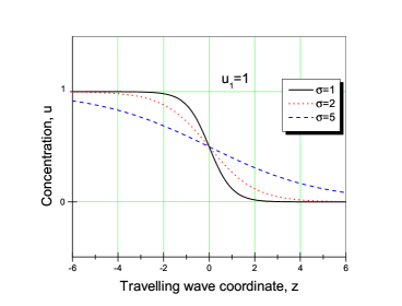
Figure 1: (Colour online) The trevelling wave front in the case of the 1st Schlögl reaction for several wave velocities $v\sim\sigma$ and $u_{1}=1$.

For the second reaction

$$V=\frac{\sigma k^{\prime}_{12}X_{1}}{2}\left(\frac{X_{1}}{2}-X_{2}\right)\,.$$ (4.17)

However, $X_{1},\,\,X_{2}$ are now the roots of quadratic equation: ${u^{2}-Ru+Q=0}$ where $R=\frac{k_{12}A}{k^{\prime}_{12}X_{0}}$ and $Q=\frac{k_{22}B}{k^{\prime}_{12}X_{0}^{2}}$. Introducing a characteristic parameter for the second reaction $\rho_{2}$,

$$\rho_{2}=4\frac{k^{\prime}_{12}k_{22}B}{\left(k_{12}A\right)^{2}};\,\,\,\,\,0<\rho_{2}<1,$$

we get

$$X_{1}=\frac{k_{12}A}{2k^{\prime}_{12}}\left[1+\sqrt{1-\rho_{2}}\right];\,\,\,\,\,X_{2}=\frac{k_{12}A}{2k^{\prime}_{12}}\left[1-\sqrt{1-\rho_{2}}\right]$$ (4.18)

and

$$V=\sigma\frac{\left(k_{12}A\right)^{2}}{16k^{\prime}_{12}}\left\{2\sqrt{1-\rho_{2}}-3\rho_{2}+2\right\}\,.$$ (4.19)

The dependence of the wave front velocity on its width $\sigma$ and parameter $\rho_{2}$ according to the above equation with $\left(k_{12}A\right)^{2}/\left(16k^{\prime}_{12}\right)=1/2$ is shown in figure 2.

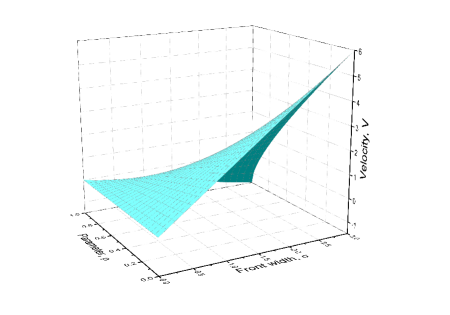
Figure 2: (Colour online) The trevelling wave front velocity in the case of 2nd Schlögl reaction as function of the front width $\sigma$ and parameter $\rho_{2}$.

Summing up, without viscosity and applied field, the constant-velocity combined-transition-front model for CHHCM is not very instructive, both transitions should be too rigidly adjusted to each other (of course, for the non-constant-velocity-fronts, the situation could be quite different). However, the presence of the field and/or viscosity changes the situation; the concentration $X$ in the final state may deviate from its equilibrium value and even the transition may be stopped. On the other hand, for the CHS equation, the effect of the non-equilibrium transition, i.e., of the reaction system, is much stronger. The transition front may be stopped, or even reversed both by changing the stationary states of the reaction system and by the field. The final state may be undersaturated or oversaturated, creating non-equilibrated phases.

Appendix A Cahn-Hilliard-Puri-Frish equation

Here, for completeness we give the exact travelling wave solution for one-dimensional version of equation, introduced by Puri and Frish [21]. To match our consideration with [21] we use their original notations and normalizations, which are different from these in the other parts of the present paper. After the correction of the evident misprint and considering the generally asymmetric thermodynamic potential, the equation (9) of [21] is

$$\frac{\partial\psi}{\partial t}=-\frac{\partial^{2}}{\partial x^{2}}\left\{\psi+\delta\psi^{2}-\psi^{3}+\frac{\partial^{2}\psi}{\partial x^{2}}\right\}-\alpha\psi\left(1-\psi\right)+\frac{\alpha}{\sigma}\psi\frac{\partial^{2}\psi}{\partial x^{2}}.$$ (A.1)

Here, $\alpha$ is a phenomenological constant, proportional to the ratio of the characteristic times for a spin exchange and reaction, $\sigma$ is proportional to the inverse square of lattice spacing. Evidently, dropping the last term in the right-hand side of (A.1) we obtain CHHCM equation, though with an inverted sign of the reaction term, see section 2. This means that for the reaction system the stable state is $\psi=0$, while $\psi=1$ is unstable. Looking for the travelling wave solutions of (A.1), we introduce the travelling wave coordinate $z=x-vt$. This yields

$$-v\frac{\mathrm{d}\psi}{\mathrm{d}z}=-\frac{\mathrm{d}^{2}}{\mathrm{d}z^{2}}\left\{\psi+\delta\psi^{2}-\psi^{3}+\frac{\mathrm{d}^{2}\psi}{\mathrm{d}z^{2}}\right\}-\alpha\psi\left(1-\psi\right)+\frac{\alpha}{\sigma}\psi\frac{\mathrm{d}^{2}\psi}{\mathrm{d}z^{2}}.$$ (A.2)

Introducing the ansatz

$$\frac{\mathrm{d}\psi}{\mathrm{d}z}=\kappa\psi\left(1-\psi\right),$$ (A.3)

which for the positive $\kappa$ and $0\leqslant\psi\leqslant 1$ corresponds to the kink-like solution, the last two terms in the right-hand side of (A.2) could be rewritten as

$$-\alpha\psi\left(1-\psi\right)+\frac{\alpha}{\sigma}\psi\frac{\mathrm{d}^{2}\psi}{\mathrm{d}z^{2}}=\frac{\mathrm{d}}{\mathrm{d}z}\left[-\frac{\alpha}{\kappa}\psi+\frac{\alpha}{2\sigma}\kappa\psi^{2}-\frac{2\alpha}{3\sigma}\kappa\psi^{3}\right].$$ (A.4)

Substituting the latter expression into (A.2), integrating once and rearranging the terms we get

$$\left(v-\frac{\alpha}{\kappa}\right)\psi+\frac{\alpha}{2\sigma}\kappa\psi^{2}-\frac{2\alpha}{3\sigma}\kappa\psi^{3}-\frac{\mathrm{d}}{\mathrm{d}z}\left(\psi+\delta\psi^{2}-\psi^{3}+\frac{\mathrm{d}^{2}\psi}{\mathrm{d}z^{2}}\right)=C_{1}.$$ (A.5)

For the latter equation to be satisfied, the expression under the derivative should be a quadratic function of $u$:

$$\psi+\delta\psi^{2}-\psi^{3}+\frac{\mathrm{d}^{2}\psi}{\mathrm{d}z^{2}}=\beta\psi+\gamma\psi^{2}+C_{2}\,,$$ (A.6)

$$\left(v-\frac{\alpha}{\kappa}\right)\psi+\frac{\alpha}{2\sigma}\kappa\psi^{2}-\frac{2\alpha}{3\sigma}\kappa\psi^{3}-\left(\beta+2\gamma\psi\right)\frac{\mathrm{d}\psi}{\mathrm{d}z}=C_{1},$$ (A.7)

where $\beta,\,\,\gamma,\,\,C_{1}$ and $C_{2}$ are constants. Substitution of the corresponding expressions for the derivatives into (A.6) and (A.7) yields

$$\left(v-\frac{\alpha}{\kappa}\right)\psi+\frac{\alpha}{2\sigma}\kappa\psi^{2}-\frac{2\alpha}{3\sigma}\kappa\psi^{3}+\kappa\left[2\gamma\psi^{3}+\left(\beta-2\gamma\right)\psi^{2}-\beta\psi\right]=C_{1},$$ (A.8)

$$\psi+\delta\psi^{2}-\psi^{3}+\kappa^{2}\left(2\psi^{3}-3\psi^{2}+\psi\right)=\beta\psi+\gamma\psi^{2}+C_{2}.$$ (A.9)

Rearranging and equating to zero coefficients at all powers of $\psi$, we obtain the system of constraints imposed on the parameters.

$$2\kappa^{2}=1,$$ (A.10)

$$\delta-\frac{3}{2}=\gamma,$$ (A.11)

$$\beta=\frac{3}{2},$$ (A.12)

$$\gamma=\frac{\alpha}{3\sigma},$$ (A.13)

$$\frac{\alpha}{2\sigma}+\beta-2\gamma=0,$$ (A.14)

$$v=\frac{\alpha}{\kappa}+\kappa\beta.$$ (A.15)

If these constraints are satisfied, the solutions of (A.3) are simultaneously the solutions of the travelling-wave equation (A.2), which, quite analogously to (2.24) is

$$\psi=\frac{1}{2}\left\{1+\tanh\left[\frac{1}{2\sqrt{2}}\left(x-vt\right)\right]\right\}.$$ (A.16)

From (A.10), (A.12) and (A.15) $v=\sqrt{2}\alpha+\frac{3}{2\sqrt{2}}$, the velocity of the kink is always positive ($\alpha$ is per definition positive), i.e., the stable $\psi=0$ state spreads on the cost of the unstable state $\psi=1$. The constraints imposed on the parameters of the model are $\alpha=9\sigma;\,\,\,\delta={9\mathord{\left/{\vphantom{92}}\right.\kern-1.2pt}2}$. Then, the roots of equation

$$\psi^{3}-\delta\psi^{2}-\psi=0$$ (A.17)

are $\psi_{1}\simeq 4,712;\,\,\psi_{2}\,=0;\,\,\,\psi_{3}\simeq-0,212$, i.e., the potential $\Phi\left(\psi\right)$ should be very far from symmetric.

Ukrainian 0

Модель Кана-Гiлiярда з реакцiями Шльогля: взаємодiя рiвноважного i нерiвноважного фазових переходiв.
I. Розв’язок типу рухомої хвилi П.О. Мчедлов-Петросян, Л.М. Давидов

             
Нацiональний науковий центр ‘‘Харкiвський фiзико-технiчний iнститут’’, Харкiв, 61108, вул. Академiчна, 1

References

- [1] Cahn J.W., Hilliard J.E., J. Chem. Phys., 1958, 28, 258–267, doi:10.1063/1.1744102.
- [2] Cahn J.W., Acta Metall., 1961, 9, 795–801, doi:10.1016/0001-6160(61)90182-1.
- [3] Novick-Cohen A., In: Handbook of Differential Equations: Evolutionary Equations, Vol. 4, Dafermos C.M., Pokorny M. (Eds.), North-Holland, 2008, 201–228, doi:10.1016/S1874-5717(08)00004-2.
- [4] Miranville A., AIMS Math., 2017, 2, No. 3, 479–544, doi:10.3934/Math.2017.2.479.
- [5] Van der Waals J.D., J. Stat. Phys., 1979, 20, 200–244, doi:10.1007/BF01011514.
- [6] De Groot S.R., Mazur P., Non-Equilibrium Thermodynamics, Dover, NY, 1984.
- [7] Novick-Cohen A., Segel L.A., Physica D, 1984, 10, 277–298.
- [8] Novick-Cohen A., In: Material Instabilities in Continuum Mechanics and Related Mathematical Problems, Ball J.M. (Ed.), Oxford Univ. Press, Oxford, 1988, 329–342.
- [9] Bai F., Elliott C.M., Gardiner A., Spence A., Stuart A.M., The Viscous Cahn-Hilliard Equation. I. Computations. Nonlinearity, 1995, 8, 131–160.
- [10] Leung K., J. Stat. Phys., 1990, 61, 345–364, doi:10.1007/BF01013969.
- [11] Witelski T.P., Appl. Math. Lett., 1995, 8, 27–32, doi:10.1016/0893-9659(95)00062-U.
- [12] Emmott C.L., Bray A.J., Phys. Rev. E, 1996, 54, No. 5, 4568–4575, doi:10.1103/PhysRevE.54.4568.
- [13] Kuramoto Y., Tsuzuki T., Prog. Theor. Phys., 1976, 55, No. 2, 356–369, doi:10.1143/PTP.55.356.
- [14] Sivashinsky G., Acta Astron., 1977, 4, 1177–1206, doi:10.1016/0094-5765(77)90096-0.
- [15] Watson S.J., Otto F., Rubinstein B.Y., Davis S.H., Max-Plank-Institut fuer Mathematik in den Naturwissenschaften, Preprint No. 35, Leipzig, 2002.
-
[16]
Watson S.J., Otto F., Rubinstein B.Y., Davis S.H., Physica D, 2003, 178, 127–148,
doi:10.1016/S0167-2789(03)00048-4. - [17] Witelski T.P., Stud. Appl. Math., 1996, 96, 277-300, doi:10.1002/sapm1996973277.
- [18] Mchedlov-Petrosyan P.O., Eur. J. Appl. Math., 2016, 27, 42–65, doi:10.1017/S0956792515000285.
- [19] Huberman B.A., J. Chem. Phys., 1976, 65, No. 5, 2013–2019, doi:10.1063/1.433272.
- [20] Cohen D.S., Murray J.D., J. Math. Biology, 1981, 12, 237–249, doi:10.1007/BF00276132.
- [21] Puri S., Frisch H.L., J. Phys. A: Math. Gen., 1994, 27, 6027–6038, doi:10.1088/0305-4470/27/18/013.
- [22] Verdasca J., Borckmans P., Dewel G., Phys. Rev. E, 1995, 52, R4616–R4619, doi:10.1103/PhysRevE.52.R4616.
- [23] Khain E., Sander L.M., Phys. Rev. E, 2008, 77, 051129, doi:10.1103/PhysRevE.77.051129.
- [24] Miranville A., Appl. Anal., 2013, 92, No. 6, 1308–1321, doi:10.1080/00036811.2012.671301.
- [25] Cherfils L., Miranville A., Zelik S., Discrete Contin. Dyn. Syst.-Ser. B, 2014, 19, No. 7, 2013–2026, doi:10.3934/dcdsb.2014.19.2013.
- [26] Schlögl F., Z. Angew. Phys., 1972, 253, 147–161, doi:10.1007/BF01379769.
Ukrainian \adddialect\l@ukrainian0 \l@ukrainian