Dynamical System Analysis of a Three Fluid Cosmological Model : An Invariant Manifold approach

Abstract

The present paper considers a three-fluid cosmological model consisting of noninteracting dark matter, dark energy and baryonic matter in the background of the Friedman-Robertson-Walker-Lemaître flat spacetime. It has been assumed that the dark matter takes the form of dust whereas the dark energy is a quintessence (real) scalar field with exponential potential. It has been further assumed that the baryonic matter is a perfect fluid with barotropic equation of states. The field equations for this model takes the form of an autonomous dynamical system after some suitable changes of variables. Then a complete stability analysis is done considering all possible parameter (the adiabatic index of the baryonic matter and the parameter arising from the dark energy potential) values and for both the cases of hyperbolic and non-hyperbolic critical points. For non-hyperbolic critical points, the invariant manifold theory (center manifold approach) is applied. Finally various topologically different phase planes and vector field diagrams are produced and the cosmological interpretation of this model is presented.

Keywords : Non-hyperbolic point, Center manifold theory, Field equations.

PACS Numbers : 98.80.-k, 05.45.-a, 02.40.Sf, 02.40.Tt

I Introduction

Recently, a large number of observational data from various sources such as Type Ia Supernova Rei98 ; Perl99 , CMB anisotropies Sper07 ; Komat09 , Large Scale Structures Teg04 ; Per01 and Baryon Acoustic Oscillations Eisen03 suggests that we are in a spatially flat universe which after the big bang has undergone two accelerated expansion phases, one occurred before the radiation dominated era and the other one started not too long ago. We are presently in this accelerated expansion phase.

This present time accelerated expansion has been attributed to a unseen and unknown matter with very large negative pressure called the dark energy. Analysis of different cosmological data suggests that our universe is composed of around $70$% dark energy, about $25$% dark matter and the rest accounts for baryonic matter and radiation.

Very few properties of the dark energy is known AT10 . As far as the mathematical modelling of this exotic matter is concerned, the simplest choice for it has been the Cosmological Constant $\Lambda$ Wein89 ; Carrol01 ; PR03 . Although these models are capable of explaining most of the observational data, all of them fails to explain the coincidence problem (why expansion is happening now and why is it accelerated) and the fine-tuning problem (why some of the parameters take exorbitantly high values where others are not). To resolve these issues, lots of dynamical dark energy models has been prescribed. There the dark energy has been modelled as a scalar field. Some scalar field models like quintessence RP88 ; CDS98 , K-essence and Tachyonic models have attracted lots of attention.

In this paper we consider a cosmological model consisting of non-interacting dark matter, dark energy and baryonic matter in the background of the Friedman-Robertson-Walker-Lemaître flat spacetime. The dark matter has been assumed to take the form of dust whereas the dark energy is assumed to be a scalar field with exponential potential. It has been further assumed that the baryonic matter is a perfect fluid with barotropic equation of states. All these three fluids are assumed to be non-interacting and minimally coupled to gravity.

In order to study this model qualitatively, we derive the Einstein’s field equations and the Klein-Gordan equation for the scalar field. After some suitable changes of variables, these equations take the form of an autonomous dynamical system. Then we find the critical points and analyze the stability of each critical point. We note that in  MC15 the model like ours have been considered. But the authors did not consider the cases of non-hyperbolic critical points. Our results differ from them in various ways. Firstly, we apply some of the very rich theories for the dynamical systems, namely the Invariant Manifold and the Center Manifold Theory  Per91 ; AP90 ; Wig03 ; ASB to compute the center manifolds for all the non-hyperbolic critical points and then continue to do the stability analysis for them. The other one is that we have considered all theoretically possible values of the parameters to do a complete analysis here, whereas in their article, they chose only a few suitable values. Lastly, we have presented all possible topologically different phase plane diagrams here where they included only some of them in their article.

The motivation to do stability analysis is that after considering all cosmological and observational constraints of data, the stable critical points in our model may depict our present universe as a global attractor. If they do fit with the data of present percentages of dark energy, dark matter and baryonic matter together with radiation in the universe then our model would successfully describe the universe.

The organization of this article is as follows : The section II describes the Einstein field equations, Klein-Gordan scalar field equation and energy conservation relations for our model. Section III describes the formation of an autonomous system. The section IV is where we present our work on complete stability analysis. At the end of this section, we produce the phase plane diagrams for different topological cases. Finally section V presents the cosmological interpretations of our results and concludes our work.

II Equations

The homogeneous and isotropic flat Friedman-Robertson-Walker-Lemaître spacetime is the background of our model. This universe is assumed to be filled up by non-interacting dark matter, dark energy and baryon. Dark matter is assumed to be dust with energy density $\rho_{m}$ and the dark energy is assumed to be a scalar field $\phi$ with the potential as $V(\phi)$. The density $\rho_{d}$ and the pressure $p_{d}$ of the scalar field follows the following equations :

$$\rho_{d}=\frac{1}{2}\dot{\phi}^{2}+V(\phi)$$ (1)

and

$$p_{d}=\frac{1}{2}\dot{\phi}^{2}-V(\phi).$$ (2)

Here $\dot{}$ denotes differentiation with respect to cosmic time $t.$

The baryonic matter is assumed to be a perfect fluid with linear equation of state

$$p_{b}=(\nu-1)\rho_{b}$$ (3)

where $p_{b}$ and $\rho_{b}$ are the density and the pressure of the fluid and $\nu$ is the adiabatic index of the fluid satisfying $\frac{2}{3}<\nu\leq 2.$ In particular $\nu=1$ and $\nu=\frac{4}{3}$ corresponds to the dust and radiation respectively. Here we also assume that $\nu\neq 1$ All three matter are non-interacting and minimally coupled to gravity.

The Einstein field equations for this model is

$$3H^{2}=k(\rho_{m}+\rho_{d}+\rho_{b}).$$ (4)

where $H$ is the Hubble parameter and $k=8\pi G$, where $G$ is the gravitational constant, the speed of light has been scaled to $1.$

The Klein-Gordan equation of the scalar field is

$$\ddot{\phi}+3H\dot{\phi}+\frac{dV}{d\phi}=0$$ (5)

The energy conservation relations take the following form

$$\dot{\rho_{m}}+3H\rho_{m}=0$$ (6)

$$\dot{\rho_{d}}+3H(\rho_{d}+p_{d})=0$$ (7)

$$\dot{\rho_{b}}+3H(\rho_{b}+p_{b})=0$$ (8)

From (4),(5),(6),(7) and (8) we derive

$$2\dot{H}=-k(\rho_{m}+\rho_{b}+p_{b}+\dot{\phi}^{2}).$$ (9)

The equations (4),(9) and (5) are the evolution equations for this model. Next we find suitable coordinate changes such that these evolution equations form a system of autonomous dynamical system. This is done in the following section.

III The autonomous system

We introduce the following coordinate transformations of variables :

$$x=\sqrt{\frac{k}{6}}\frac{\dot{\phi}}{H},$$ (10)

$$y=\sqrt{\frac{k}{3}}\frac{\sqrt{V(\phi)}}{H}$$ (11)

and the density parameters

$$\Omega_{m}=\frac{k\rho_{m}}{3H^{2}},$$ (12)

$$\Omega_{b}=\frac{k\rho_{b}}{3H^{2}},$$ (13)

$$\Omega_{d}=\frac{k\rho_{d}}{3H^{2}}.$$ (14)

These coordinate changes transform the Friedmann equation (4) and the equation (9) respectively as the following :

$$\Omega_{d}=x^{2}+y^{2},$$ (15)

$$\Omega_{m}+\Omega_{b}+x^{2}+y^{2}=1$$ (16)

and

$$\dot{H}=-3H^{2}(x^{2}+\frac{\Omega_{m}}{2}+\nu\frac{\Omega_{b}}{2}).$$ (17)

As $\Omega_{m}$ and $\Omega_{b},$ the density parameters are non-negative real quantities, so from (16) $0\leq\Omega_{m}\leq 1,0\leq\Omega_{b}\leq 1$ and $x$ and $y$ satisfies $x^{2}+y^{2}\leq 1.$ The strict equality is only possible if the energy densities of the dark matter and the baryonic matter is zero.

Differentiating the equations (10), (11) and (12) with respect to $N$ where $N=\ln a$ ($a(t)$ is the scale factor of the universe) and using (16), (17), (5) and (6), (7) and (8) we derive the following autonomous dynamical system :

$$\frac{dx}{dN}=3x[x^{2}-1+\frac{\Omega_{m}}{2}+\frac{\nu}{2}(1-\Omega_{m}-x^{2}-y^{2})]-\sqrt{\frac{3}{2k}}\frac{1}{V}\frac{dV}{d\phi}y^{2}$$ (18)

$$\frac{dy}{dN}=y[3x^{2}+3\frac{\nu}{2}(1-\Omega_{m}-x^{2}-y^{2})+3\frac{\Omega_{m}}{2}+\sqrt{\frac{3}{2k}}\frac{1}{V}\frac{dV}{d\phi}x]$$ (19)

$$\frac{d\Omega_{m}}{dN}=-3\Omega_{m}[1-\Omega_{m}-2x^{2}-\nu(1-\Omega_{m}-x^{2}-y^{2})]$$ (20)

We end this section by expressing the relevant cosmological parameters in terms of the above transformed variables as

$$\Omega_{d}=x^{2}+y^{2},$$ (21)

$$\omega_{d}=\frac{p_{d}}{\rho_{d}}=\frac{x^{2}-y^{2}}{x^{2}+y^{2}},$$ (22)

$$\omega_{eff}=\frac{p_{d}+p_{b}}{\rho_{m}+\rho_{d}+\rho_{b}}=-1+2x^{2}+\nu(1-\Omega_{m}-x^{2}-y^{2})+\Omega_{m}$$ (23)

and

$$q=-(1+\frac{\dot{H}}{H^{2}})=-[(1-3x^{2}-\frac{3\nu}{2})-\frac{3\Omega_{m}}{2}(1-\nu)+\frac{3\nu}{2}(x^{2}+y^{2})].$$ (24)

We note that for accelerated expansion, $\omega_{eff}\leq-\frac{1}{3}$ and $q\leq 0$ are two necessary conditions.

IV Stability Analysis

We start working on the stability analysis of the dynamical system (18) in this section. We assume that the potential of the scalar field representing the dark energy is exponential, ie $\frac{1}{V}\frac{dV}{d\phi}=$ some constant. We choose $\sqrt{\frac{3}{2k}}\frac{1}{V}\frac{dV}{d\phi}=\alpha.$ Then the autonomous system (18) transforms into :

$$\frac{dx}{dN}=3x[x^{2}-1+\frac{\Omega_{m}}{2}+\frac{\nu}{2}(1-\Omega_{m}-x^{2}-y^{2})]-\alpha y^{2}$$ (25)

$$\frac{dy}{dN}=y[3x^{2}+3\frac{\nu}{2}(1-\Omega_{m}-x^{2}-y^{2})+3\frac{\Omega_{m}}{2}+\alpha x]$$ (26)

$$\frac{d\Omega_{m}}{dN}=-3\Omega_{m}[1-\Omega_{m}-2x^{2}-\nu(1-\Omega_{m}-x^{2}-y^{2})]$$ (27)

There are ten critical points of this autonomous system. They are listed in the table below.

Table 1: Critical Points

Critical Point Name	Critical Point
$C_{1}$	$(0,0,0)$
$C_{2}$	$(1,0,0)$
$C_{3}$	$(0,0,1)$
$C_{4}$	$(-1,0,0)$
$C_{5}$	$(-\frac{\alpha}{3},\frac{1}{3}\sqrt{9-\alpha^{2}},0)$
$C_{6}$	$(-\frac{\alpha}{3},-\frac{1}{3}\sqrt{9-\alpha^{2}},0)$
$C_{7}$	$(-\frac{3\nu}{2\alpha},\frac{3}{2\alpha}\sqrt{2\nu-\nu^{2}},0)$
$C_{8}$	$(-\frac{3\nu}{2\alpha},-\frac{3}{2\alpha}\sqrt{2\nu-\nu^{2}},0)$
$C_{9}$	$(-\frac{3}{2\alpha},\frac{3}{2\alpha},(1-\frac{9}{2\alpha^{2}}))$
$C_{10}$	$(-\frac{3}{2\alpha},-\frac{3}{2\alpha},(1-\frac{9}{2\alpha^{2}}))$

The value of the relevant cosmological parameters for each of the critical points are given in the following table :

Table 2: Values of the Different Cosmological Parameters at the Critical Points

Critical Points	$\omega_{d}$	$\omega_{eff}$	$\Omega_{m}$	$\Omega_{d}$	$\Omega_{b}$	$q$
$C_{1}$	Undefined	$\nu-1$	$0$	$0$	$1$	$\frac{3\nu}{2}-1$
$C_{2}$	$1$	$1$	$0$	$1$	$0$	$2$
$C_{3}$	Undefined	$0$	$1$	$0$	$0$	$\frac{1}{2}$
$C_{4}$	$1$	$1$	$0$	$1$	$0$	$2$
$C_{5}$	$\frac{2\alpha^{2}}{9}-1$	$\frac{2\alpha^{2}}{9}-1$	$0$	$1$	$0$	$\frac{\alpha^{2}}{3}-1$
$C_{6}$	$\frac{2\alpha^{2}}{9}-1$	$\frac{2\alpha^{2}}{9}-1$	$0$	$1$	$0$	$\frac{\alpha^{2}}{3}-1$
$C_{7}$	$\nu-1$	$\nu-1$	$0$	$\frac{9\nu}{2\alpha^{2}}$	$1-\frac{9\nu}{2\alpha^{2}}$	$\frac{3\nu}{2}-1$
$C_{8}$	$\nu-1$	$\nu-1$	$0$	$\frac{9\nu}{2\alpha^{2}}$	$1-\frac{9\nu}{2\alpha^{2}}$	$\frac{3\nu}{2}-1$
$C_{9}$	$0$	$0$	$1-\frac{9}{2\alpha^{2}}$	$\frac{9}{2\alpha^{2}}$	$0$	$\frac{1}{2}$
$C_{10}$	$0$	$0$	$1-\frac{9}{2\alpha^{2}}$	$\frac{9}{2\alpha^{2}}$	$0$	$\frac{1}{2}$

For every critical point and for each of their subcases we will do two successive change of variables to bring them to a form with which the calculation of center manifold and dynamics of the reduced system will be easy. For each of the cases and subcases the transformations are as follows :

If

$X=\left(\begin{array}[]{c}x\\ y\\ \Omega_{m}\\ \end{array}\right),$ $\bar{X}=\left(\begin{array}[]{c}\bar{x}\\ \bar{y}\\ \bar{\Omega_{m}}\\ \end{array}\right)$ and $\bar{\bar{X}}=\left(\begin{array}[]{c}\bar{\bar{x}}\\ \bar{\bar{y}}\\ \bar{\bar{\Omega_{m}}}\\ \end{array}\right),$

then $\bar{X}=X-A$ and $\bar{\bar{X}}=P^{-1}\bar{X}$ where $A$ and $P$ is some $3\times 1$ and $3\times 3$ matrices respectively with $P$ being non-singular. The exact form of $A$ and $P$ will vary from case to case and we will mention them while studying each of the cases and subcases.

IV.1 Critical Point $C_{1}$

For critical point $C_{1}$, $A=\left(\begin{array}[]{c}0\\ 0\\ 0\\ \end{array}\right)$ and the Jacobian matrix of the system (25) at this critical point has the characteristic polynomial

$$\lambda^{3}+(6-6\nu)\lambda^{2}+[\frac{3\nu(3\nu-3)}{2}+\frac{(3\nu-6)(9\nu-6)}{4}]\lambda-\frac{3\nu(3\nu-3)(3\nu-6)}{4}=0.$$ (28)

which has eigen values as $3\nu-3,\frac{3\nu}{2}-3$ and $\frac{3\nu}{2}.$ The stability analysis when $\nu$ is not $0,1$ or $2$ (hyperbolic cases) is an easy application of the stability analysis of the linear system and the Hartman-Gröbman Theorem.

So now we will present a table containing the non-hyperbolic subcases and the result of their stability analysis. Later We will write the stability results for all possible subcases for $C_{1}$.

Before we write down the table, we introduce a notation. ^′ represents derivative with respect to $N.$

Table 3: $C_{1}$(Reduced System)

$\nu$	Center Manifold	Reduced System
$0$	$\bar{\bar{x}}=O(\bar{\bar{\Omega_{m}}}^{3}),\bar{\bar{y}}=-\frac{\alpha}{3}\bar{\bar{\Omega_{m}}}^{2}+O(\bar{\bar{\Omega_{m}}}^{3})$	$\bar{\bar{\Omega_{m}}}^{\prime}=-\frac{\alpha^{2}}{3}\bar{\bar{\Omega_{m}}}^{3}+O(\bar{\bar{\Omega_{m}}}^{4})$
$1$	$\bar{\bar{y}}=O(\bar{\bar{x}}^{3}),\bar{\bar{\Omega_{m}}}=O(\bar{\bar{x}}^{3})$	$\bar{\bar{x}}^{\prime}=0$
$2$	$\bar{\bar{x}}=O(\bar{\bar{y}}^{3}),\bar{\bar{\Omega_{m}}}=O(\bar{\bar{y}}^{3})$	$\bar{\bar{y}}^{\prime}=0$

For all these subcases, $P=\left(\begin{array}[]{ccc}0&1&0\\ 0&0&1\\ 1&0&0\\ \end{array}\right).$

We summarize our results for $C_{1}$ in the table below to end this subsection.

Table 4: Summary for the critical point $C_{1}$

Case	$\nu$	Stability(RS)	Stability(DS)
a	$\nu<0$	NA	Stable
b	$\nu=0$	Stable	Stable
c	$0<\nu<1$	NA	Saddle
d	$\nu=1$	Center	Center-Saddle
e	$1<\nu<2$	NA	Saddle
f	$\nu=2$	Center	Center-Unstable
g	$2<\nu$	NA	Unstable

Here RS stands for the Reduced System, DS stands for the whole system and NA stands for Not Applicable (Hyperbolic Cases).

IV.2 Critical Point $C_{2}$

For critical point $C_{2}$, $A=\left(\begin{array}[]{c}1\\ 0\\ 0\\ \end{array}\right)$ and the Jacobian matrix of the system (25) at this critical point has the characteristic polynomial

$$\lambda^{3}+(3\nu-\alpha-12)\lambda^{2}+[18-(3\nu-9)(\alpha+3)-9\nu]\lambda-(9\nu-18)(\alpha+3)=0.$$ (29)

which has eigen values as $3,6-3\nu$ and $\alpha+3.$ The stability analysis when $\nu$ is not $2$ and $\alpha$ is not $-3$ (hyperbolic cases) is again an easy application of the stability analysis of the linear system and the Hartman-Gröbman Theorem.

So we will present a table containing all the non-hyperbolic subcases and the result of their stability analysis. Later We will write the stability results for all possible subcases for $C_{2}$.

Table 5: $C_{2}$(Reduced System)

$\nu$	$\alpha$	Center Manifold	Reduced System
$2$	$-3$	$\bar{\bar{\Omega_{m}}}=O(\parallel(\bar{\bar{x}},\bar{\bar{y}})\parallel^{3})$	$\bar{\bar{x}}^{\prime}=-3\bar{\bar{x}}\bar{\bar{y}}^{2},\bar{\bar{y}}^{\prime}=-3\bar{\bar{x}}\bar{\bar{y}}$
$2$	$\neq-3$	$\bar{\bar{y}}=O(\bar{\bar{x}}^{3}),\bar{\bar{\Omega_{m}}}=O(\bar{\bar{x}}^{3})$	$\bar{\bar{x}}^{\prime}=0$
$\neq 2$	$-3$	$\bar{\bar{y}}=O(\bar{\bar{x}}^{3}),\bar{\bar{\Omega_{m}}}=-\frac{1}{2}\bar{\bar{x}}^{2}+O(\bar{\bar{x}}^{3})$	$\bar{\bar{x}}^{\prime}=-\frac{3}{2}\bar{\bar{x}}^{3}$

When $\nu=2$ and $\alpha=-3$ the $P$ is $\left(\begin{array}[]{ccc}1&0&-\frac{1}{2}\\ 0&1&0\\ 0&0&1\\ \end{array}\right).$

For $\nu=2$ and $\alpha\neq-3,$ $P=\left(\begin{array}[]{ccc}1&-\frac{1}{2}&0\\ 0&0&1\\ 0&1&0\\ \end{array}\right).$

When $\nu\neq 2$ and $\alpha=-3$ then $P=\left(\begin{array}[]{ccc}0&-\frac{1}{2}&1\\ 1&0&0\\ 0&1&0\\ \end{array}\right).$

We end this subsection by summarizing our results for $C_{2}$ in a table.

Table 6: A summary for the critical point $C_{2}$

Case	$\nu$	$\alpha$	Stability(RS)	Stability(DS)
a	$<2$	$<-3$	NA	Saddle
b	$<2$	$-3$	Stable	Saddle
c	$<2$	$>-3$	NA	Unstable
d	$2$	$>-3$	Center	Center-Unstable
e	$2$	$-3$	Stable	Saddle
f	$2$	$<-3$	Center	Center-Saddle
g	$>2$	$<-3$	NA	Saddle
h	$>2$	$-3$	Stable	Saddle
i	$>2$	$>-3$	NA	Saddle

IV.3 Critical Point $C_{3}$

For $C_{3}$ the $A=\left(\begin{array}[]{c}0\\ 0\\ 1\\ \end{array}\right).$

The Jacobian Matrix at $C_{3}$ has the characteristic polynomial

$$\lambda^{3}+(3\nu-3)\lambda^{2}-\frac{9}{4}\lambda+[\frac{27}{4}-\frac{27\nu}{4}]=0$$ (30)

which has the eigenvalues $-\frac{3}{2},\frac{3}{2}$ and $3-3\nu.$

Hence the stability analysis is almost trivial if $\nu\neq 1.$ Because then it is an immediate application of the stability analysis of the linear cases and the Hartman-Gröbman theorem.

Therefore we assume that $\nu=1$ and proceed with our stability analysis.

Table 7: $C_{3}$(Reduced System)

$\nu$	Center Manifold	Reduced System
$1$	$\bar{\bar{y}}=O(\bar{\bar{x}}^{3}),\bar{\bar{\Omega_{m}}}=O(\bar{\bar{x}}^{3})$	$\bar{\bar{x}}^{\prime}=0$

For this subcase $P$ is $\left(\begin{array}[]{ccc}0&0&1\\ 0&1&0\\ 1&0&0\\ \end{array}\right).$

At the end, here is the summary of the results for $C_{3}.$

Table 8: The critical point $C_{3},$ a summary

Case	$\nu$	Stability(RS)	Stability(DS)
a	$<1$	NA	Saddle
b	$1$	Center	Center-Saddle
c	$>1$	NA	Saddle

IV.4 Critical Point $C_{4}$

For critical point $C_{4}$, $A=\left(\begin{array}[]{c}-1\\ 0\\ 0\\ \end{array}\right)$ and the Jacobian matrix of the system (25) at this critical point has the characteristic polynomial

$$\lambda^{3}+(3\nu+\alpha-12)\lambda^{2}+[(3\nu-6)(\alpha-6)-3\alpha+9]\lambda-(3\nu-6)(3\alpha-9)=0.$$ (31)

which has eigen values as $3,6-3\nu$ and $3-\alpha.$ The stability analysis when $\nu$ is not $2$ and $\alpha$ is not $3$ (hyperbolic cases) is easy again as said before.

Now we will present a table containing all the non-hyperbolic subcases and the result of their stability analysis. Later We will write the stability results for all possible subcases for $C_{4}$.

Table 9: $C_{4}$(reduced System)

$\nu$	$\alpha$	Center Manifold	Reduced System
$2$	$3$	$\bar{\bar{\Omega_{m}}}=O(\parallel(\bar{\bar{x}},\bar{\bar{y}})\parallel^{3})$	$\bar{\bar{x}}^{\prime}=-3\bar{\bar{x}}\bar{\bar{y}}^{2},\bar{\bar{y}}^{\prime}=3\bar{\bar{x}}\bar{\bar{y}}$
$2$	$\neq 3$	$\bar{\bar{y}}=O(\bar{\bar{x}}^{3}),\bar{\bar{\Omega_{m}}}=O(\bar{\bar{x}}^{3})$	$\bar{\bar{x}}^{\prime}=0$
$\neq 2$	$3$	$\bar{\bar{y}}=O(\bar{\bar{x}}^{3}),\bar{\bar{\Omega_{m}}}=\frac{1}{2}\bar{\bar{x}}^{2}+O(\bar{\bar{x}}^{3})$	$\bar{\bar{x}}^{\prime}=-\frac{3}{2}\bar{\bar{x}}^{3}$

When $\nu=2$ and $\alpha=3$ the $P$ is $\left(\begin{array}[]{ccc}1&0&\frac{1}{2}\\ 0&1&0\\ 0&0&1\\ \end{array}\right).$

For $\nu=2$ and $\alpha\neq 3,$ $P=\left(\begin{array}[]{ccc}1&\frac{1}{2}&0\\ 0&0&1\\ 0&1&0\\ \end{array}\right).$

When $\nu\neq 2$ and $\alpha=3$ then $P=\left(\begin{array}[]{ccc}0&\frac{1}{2}&1\\ 1&0&0\\ 0&1&0\\ \end{array}\right).$

We end this subsection by summarizing our results for $C_{4}$ in a table.

Table 10: $C_{4},$ a stability analysis

Case	$\nu$	$\alpha$	Stability(RS)	Stability(DS)
a	$<2$	$<3$	NA	Unstable
b	$<2$	$3$	Stable	Saddle
c	$<2$	$>3$	NA	Saddle
d	$2$	$>3$	Center	Center-Saddle
e	$2$	$3$	Stable	Saddle
f	$2$	$<3$	Center	Center-Unstable
g	$>2$	$<3$	NA	Saddle
h	$>2$	$3$	Stable	Saddle
i	$>2$	$>3$	NA	Saddle

IV.5 Critical Point $C_{5}$

Here it is necessary that $\mid\alpha\mid\leq 3.$

$A$=$\left(\begin{array}[]{c}-\frac{\alpha}{3}\\ \frac{1}{3}\sqrt{9-\alpha^{2}}\\ $0$\\ \end{array}\right)$

for this case.

The Jacobian matrix of the system (25) at this critical point has the characteristic polynomial

$$\lambda^{3}+(3\nu-\frac{5}{3}\alpha^{2}+6)\lambda^{2}+[18\nu-3\nu\alpha^{2}-7\alpha^{2}+\frac{8}{9}\alpha^{4}+9]\lambda-\frac{(9\nu-2\alpha^{2})(2\alpha^{4}-27\alpha^{2}+81)}{27}=0.$$ (32)

This characteristic polynomial has eigenvalues as $\frac{2\alpha^{3}}{3}-3\nu,\frac{\alpha^{2}}{3}-3$ and $\frac{2\alpha^{3}}{3}-3.$ The stability analysis when $\nu\neq\frac{2\alpha^{2}}{9}$ and $\alpha\neq\pm 3,\pm\frac{3}{\sqrt{2}}$ (hyperbolic cases) is easy as said in the above subsections.

Now we will present a table containing all the non-hyperbolic subcases and the result of their stability analysis. Since for $C_{5},$ the total number of all possible subcases is too many, we would not present the results for the complete case in a table at the end as we did in the previous subsections. We would rather present a diagram in $\alpha-\nu$ plane to show the stability analysis for all possible values of $\alpha$’s and $\nu$’s.

Table 11: $C_{5}$(Reduced System)

$\nu$	$\alpha$	Center Manifold	Reduced System
$2$	$3$	id to subcase (e) of $C_{4}$	id to subcase (e) of $C_{4}$
$\neq 2$	$3$	id to subcase (b) and (h) of $C_{4}$	id to subcase (b) and (h) of $C_{4}$
$2$	$-3$	id to subcase (e) of $C_{2}$	id to subcase (e) of $C_{2}$
$\neq 2$	$-3$	id to subcase (b) and (h) of $C_{2}$	id to subcase (b) and (h) of $C_{2}$
$1$	$\frac{3}{\sqrt{2}}$	$\bar{\bar{\Omega_{m}}}=\frac{1}{\sqrt{2}}\bar{\bar{x}}^{2}+O(\parallel(\bar{\bar{x}},\bar{\bar{y}})\parallel^{3})$	$\bar{\bar{x}}^{\prime}=-3\sqrt{2}\bar{\bar{x}}^{2},\bar{\bar{y}}^{\prime}=-3\sqrt{2}\bar{\bar{x}}\bar{\bar{y}}$
$\neq 1$	$\frac{3}{\sqrt{2}}$	$\bar{\bar{x}}=r\bar{\bar{y}}^{2}+O(\bar{\bar{y}}^{3}),\bar{\bar{\Omega_{m}}}=s\bar{\bar{y}}^{2}+O(\bar{\bar{y}}^{3})$	$\bar{\bar{y}}^{\prime}=-3\bar{\bar{y}}^{2}$
$1$	$-\frac{3}{\sqrt{2}}$	$\bar{\bar{\Omega_{m}}}=\frac{1}{\sqrt{2}}\bar{\bar{x}}^{2}+O(\parallel(\bar{\bar{x}},\bar{\bar{y}})\parallel^{3})$	$\bar{\bar{x}}^{\prime}=3\sqrt{2}\bar{\bar{x}}^{2},\bar{\bar{y}}^{\prime}=3\sqrt{2}\bar{\bar{x}}\bar{\bar{y}}$
$\neq 1$	$-\frac{3}{\sqrt{2}}$	$\bar{\bar{x}}=r\bar{\bar{y}}^{2}+O(\bar{\bar{y}}^{3}),\bar{\bar{\Omega_{m}}}=s\bar{\bar{y}}^{2}+O(\bar{\bar{y}}^{3})$	$\bar{\bar{y}}^{\prime}=-3\bar{\bar{y}}^{2}$
$\frac{2\alpha^{2}}{9}$	$\alpha$	$\bar{\bar{y}}=t\bar{\bar{x}}^{2}+O(\bar{\bar{x}}^{3}),\bar{\bar{\Omega_{m}}}=O(\bar{\bar{x}}^{3})$	$\bar{\bar{x}}^{\prime}=-u\bar{\bar{x}}^{2}+O(\bar{\bar{x}}^{3})$
$0$	$0$	$\bar{\bar{y}}=O(\bar{\bar{x}}^{3}),\bar{\bar{\Omega_{m}}}=O(\bar{\bar{x}}^{3})$	$\bar{\bar{x}}^{\prime}=O(\bar{\bar{x}}^{3})$

Where ”id” means ”identical” and $r=\frac{\sqrt{2}(3\nu-4)}{4(2\nu-3)}$, $s=\frac{\sqrt{2}(1-\nu)}{4(2\nu-3)}$, $t=\frac{3\sqrt{9-\alpha^{2}}(9\alpha^{2}-4\alpha^{4})}{4\alpha^{6}-72\alpha^{4}+405\alpha^{2}-729}$ and $u=-\frac{4\alpha^{2}\sqrt{9-\alpha^{2}}}{2\alpha^{2}-9}.$ We also note that in the subcase before the last one in the table, the ordered pair $(\nu,\alpha)$ is not permitted to take the values $(2,3),(2,-3),(1,\frac{3}{\sqrt{2}})$ and $(1,-\frac{3}{\sqrt{2}}).$

When $\nu=1$ and $\alpha=\frac{3}{\sqrt{2}}$ the $P$ is $\left(\begin{array}[]{ccc}1&0&1\\ 0&0&1\\ 0&1&0\\ \end{array}\right).$

For $\nu\neq 1$ and $\alpha=\frac{3}{\sqrt{2}},$ $P=\left(\begin{array}[]{ccc}1&\frac{1}{\sqrt{2}}&\frac{2-\nu}{\nu-1}\\ 1&0&1\\ 0&1&0\\ \end{array}\right).$

For $\nu=1$ and $\alpha=-\frac{3}{\sqrt{2}}$ the $P$ is $\left(\begin{array}[]{ccc}1&0&-1\\ 0&0&1\\ 0&1&0\\ \end{array}\right)$

and when $\nu\neq 1$ and $\alpha=-\frac{3}{\sqrt{2}},$ $P=\left(\begin{array}[]{ccc}-1&-\frac{1}{\sqrt{2}}&-\frac{2-\nu}{\nu-1}\\ 1&0&1\\ 0&1&0\\ \end{array}\right).$

Also in the final two subcases $P=\left(\begin{array}[]{ccc}-\frac{2\alpha(9-\alpha^{2})^{3/2}}{2\alpha^{4}-27\alpha^{2}+81}&\frac{\sqrt{9-\alpha^{2}}}{\alpha}&\frac{3}{2\alpha}\\ 1&1&0\\ 0&0&1\\ \end{array}\right)$

and $P=\left(\begin{array}[]{ccc}1&0&0\\ 0&-\frac{1}{2}&1\\ 0&1&0\\ \end{array}\right)$

respectively.

Since we will find that the stability diagram for $C_{5}$ and $C_{6}$ is identical, it will be presented at the end of the next subsection. We now proceed with the next subsection.

IV.6 Critical Point $C_{6}$

Here it is also necessary that $\mid\alpha\mid\leq 3.$

$A$=$\left(\begin{array}[]{c}-\frac{\alpha}{3}\\ -\frac{1}{3}\sqrt{9-\alpha^{2}}\\ $0$\\ \end{array}\right)$ in this case.

The Jacobian matrix of the system (25) at this critical point has the characteristic polynomial

$$\lambda^{3}+(3\nu-\frac{5}{3}\alpha^{2}+6)\lambda^{2}+[18\nu-3\nu\alpha^{2}-7\alpha^{2}+\frac{8}{9}\alpha^{4}+9]\lambda+\frac{(9\nu-2\alpha^{2})(2\alpha^{4}-27\alpha^{2}+81)}{27}=0.$$ (33)

This characteristic polynomial has eigenvalues as $\frac{2\alpha^{3}}{3}-3\nu,\frac{\alpha^{2}}{3}-3$ and $\frac{2\alpha^{3}}{3}-3.$ The stability analysis when $\nu\neq\frac{2\alpha^{2}}{9}$ and $\alpha\neq\pm 3,\pm\frac{3}{\sqrt{2}}$ (hyperbolic cases) is again easy.

Now we will present a table containing all the non-hyperbolic subcases and the result of their stability analysis. For $C_{6}$ too the total number of all possible subcases is many, so we would not present the results for the complete case in a table. We would rather present a diagram in $\alpha-\nu$ plane to show the stability analysis for all possible values of $\alpha$’s and $\nu$’s as we did for $C_{5}$.

Table 12: $C_{6}$(Reduced System)

$\nu$	$\alpha$	Center Manifold	Reduced System
$2$	$3$	id to subcase (e) of $C_{4}$	id to subcase (e) of $C_{4}$
$\neq 2$	$3$	id to subcase (b) and (h) of $C_{4}$	id to subcase (b) and (h) of $C_{4}$
$2$	$-3$	id to subcase (e) of $C_{2}$	id to subcase (e) of $C_{2}$
$\neq 2$	$-3$	id to subcase (b) and (h) of $C_{2}$	id to subcase (b) and (h) of $C_{2}$
$1$	$\frac{3}{\sqrt{2}}$	$\bar{\bar{\Omega_{m}}}=-\frac{1}{\sqrt{2}}\bar{\bar{x}}^{2}+O(\parallel(\bar{\bar{x}},\bar{\bar{y}})\parallel^{3})$	$\bar{\bar{x}}^{\prime}=-3\sqrt{2}\bar{\bar{x}}^{2},\bar{\bar{y}}^{\prime}=-3\sqrt{2}\bar{\bar{x}}\bar{\bar{y}}$
$\neq 1$	$\frac{3}{\sqrt{2}}$	$\bar{\bar{x}}=-r\bar{\bar{y}}^{2}+O(\bar{\bar{y}}^{3}),\bar{\bar{\Omega_{m}}}=-s\bar{\bar{y}}^{2}+O(\bar{\bar{y}}^{3})$	$\bar{\bar{y}}^{\prime}=-3\bar{\bar{y}}^{2}$
$1$	$-\frac{3}{\sqrt{2}}$	$\bar{\bar{\Omega_{m}}}=-\frac{1}{\sqrt{2}}\bar{\bar{x}}^{2}+O(\parallel(\bar{\bar{x}},\bar{\bar{y}})\parallel^{3})$	$\bar{\bar{x}}^{\prime}=3\sqrt{2}\bar{\bar{x}}^{2},\bar{\bar{y}}^{\prime}=3\sqrt{2}\bar{\bar{x}}\bar{\bar{y}}$
$\neq 1$	$-\frac{3}{\sqrt{2}}$	$\bar{\bar{x}}=-r\bar{\bar{y}}^{2}+O(\bar{\bar{y}}^{3}),\bar{\bar{\Omega_{m}}}=-s\bar{\bar{y}}^{2}+O(\bar{\bar{y}}^{3})$	$\bar{\bar{y}}^{\prime}=-3\bar{\bar{y}}^{2}$
$\frac{2\alpha^{2}}{9}$	$\alpha$	$\bar{\bar{y}}=-t\bar{\bar{x}}^{2}+O(\bar{\bar{x}}^{3}),\bar{\bar{\Omega_{m}}}=O(\bar{\bar{x}}^{3})$	$\bar{\bar{x}}^{\prime}=u\bar{\bar{x}}^{2}+O(\bar{\bar{x}}^{3})$
$0$	$0$	$\bar{\bar{y}}=O(\bar{\bar{x}}^{3}),\bar{\bar{\Omega_{m}}}=O(\bar{\bar{x}}^{3})$	$\bar{\bar{x}}^{\prime}=O(\bar{\bar{x}}^{3})$

Where $r,s,t$ and $u$ take usual values as defined in the subsection of $C_{5}.$ As like in the previous subsection here is also in the subcase before the last one in the table, the ordered pair $(\nu,\alpha)$ is not permitted to take the values $(2,3),(2,-3),(1,\frac{3}{\sqrt{2}})$ and $(1,-\frac{3}{\sqrt{2}}).$

When $\nu=1$ and $\alpha=\frac{3}{\sqrt{2}},$ $P=\left(\begin{array}[]{ccc}1&0&-1\\ 0&0&1\\ 0&1&0\\ \end{array}\right).$

For $\nu\neq 1$ and $\alpha=\frac{3}{\sqrt{2}},$ $P=\left(\begin{array}[]{ccc}-1&\frac{1}{\sqrt{2}}&-\frac{2-\nu}{\nu-1}\\ 1&0&1\\ 0&1&0\\ \end{array}\right).$

For $\nu=1$ and $\alpha=-\frac{3}{\sqrt{2}},$ $P=\left(\begin{array}[]{ccc}1&0&1\\ 0&0&1\\ 0&1&0\\ \end{array}\right)$

and when $\nu\neq 1$ and $\alpha=-\frac{3}{\sqrt{2}},$ $P=\left(\begin{array}[]{ccc}1&-\frac{1}{\sqrt{2}}&\frac{2-\nu}{\nu-1}\\ 1&0&1\\ 0&1&0\\ \end{array}\right).$

Also in the final two subcases $P=\left(\begin{array}[]{ccc}\frac{2\alpha(9-\alpha^{2})^{3/2}}{2\alpha^{4}-27\alpha^{2}+81}&-\frac{\sqrt{9-\alpha^{2}}}{\alpha}&\frac{3}{2\alpha}\\ 1&1&0\\ 0&0&1\\ \end{array}\right)$

and $P=\left(\begin{array}[]{ccc}1&0&0\\ 0&-\frac{1}{2}&1\\ 0&1&0\\ \end{array}\right)$

respectively.

We finish this subsection by producing the stability diagram for both $C_{5}$ and $C_{6}$ in $\alpha-\nu$ plane in the following :

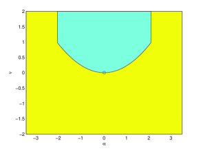
Figure 1: Stability Diagram ($C_{5},C_{6}$)

Here the cyan shaded area ie the area bounded by $\alpha=\frac{3}{\sqrt{2}},\alpha=-\frac{3}{\sqrt{2}}$ and $\nu=\frac{2\alpha^{2}}{9}$ represents the $\alpha-\nu$ pairs for which (25) is stable. The yellow shaded region represents parameter values for which (25) is saddle. Lastly the origin is center-stable here.

IV.7 Critical Point $C_{7}$

In this case, it is necessary that $0\leq\nu\leq 2$ and $\alpha\neq 0.$

$A$ takes the form $\left(\begin{array}[]{c}-\frac{3\nu}{2\alpha}\\ \frac{3\sqrt{\nu(2-\nu)}}{2\alpha}\\ $0$\\ \end{array}\right).$

The Jacobian matrix of the system (25) at $C_{7}$ has the following characteristic polynomial:

$$\lambda^{3}+(6-\frac{9\nu}{2})\lambda^{2}+[\frac{9(\nu-2)(9\nu^{2}-2\alpha^{2})}{4\alpha^{2}}]\lambda-\frac{27\nu(9\nu-2\alpha^{2})(\nu^{2}-3\nu+2)}{4\alpha^{2}}=0.$$ (34)

It has eigenvalues as $3(\nu-1),\frac{3}{4\alpha}(\nu\alpha-2\alpha+\sqrt{(2-\nu)(36\nu^{2}-9\nu\alpha^{2}+2\alpha^{2})})$ and $\frac{3}{4\alpha}(\nu\alpha-2\alpha-\sqrt{(2-\nu)(36\nu^{2}-9\nu\alpha^{2}+2\alpha^{2})}).$ The stability analysis when $\nu\neq 1,\nu\neq\frac{2\alpha^{2}}{9}$ and $\nu\neq 2,\nu\neq 0$ (hyperbolic cases) are easy by application of linear stability analysis and reduction of non-linear case to linear case under some specific conditions.

So we present a table containing all the non-hyperbolic subcases. For $C_{7}$ also, we will present a diagram in $\alpha-\nu$ plane to show the stability analysis for all possible values of $\alpha$’s and $\nu$’s at the end.

Table 13: $C_{7}$(Reduced System)

$\nu$	$\alpha$	Center Manifold	Reduced System
$1$	$\frac{3}{\sqrt{2}}$	id to subcase (e) of $C_{5}$	id to subcase (e) of $C_{5}$
$1$	$-\frac{3}{\sqrt{2}}$	id to subcase (g) of $C_{6}$	id to subcase (g) of $C_{6}$
$\neq 1$	$\nu=\frac{2\alpha^{2}}{9},\alpha>0$	id to subcase (i) of $C_{5}$	id to subcase (i) of $C_{5}$
$\neq 1$	$\nu=\frac{2\alpha^{2}}{9},\alpha<0$	id to subcase (i) of $C_{6}$	id to subcase (i) of $C_{6}$
$1$	$\nu\neq\frac{2\alpha^{2}}{9}$	$\bar{\bar{y}}=O(\bar{\bar{x}}^{3}),\bar{\bar{\Omega_{m}}}=O(\bar{\bar{x}}^{3})$	$\bar{\bar{x}}^{\prime}=0$
$2$	$\alpha$	$\bar{\bar{x}}=O(\parallel(\bar{\bar{y}},\bar{\bar{\Omega_{m}}})\parallel^{3})$	$\bar{\bar{y}}^{\prime}=\alpha\bar{\bar{y}}\bar{\bar{\Omega_{m}}},\bar{\bar{\Omega_{m}}}^{\prime}=-v\bar{\bar{y}}^{2}$
$0$	$\alpha$	id to subcase (a) of $C_{1}$	id to subcase (a) of $C_{1}$

where $v=\frac{4\alpha^{2}-36}{4\alpha}.$

For the last two subcases $P$ is $\left(\begin{array}[]{ccc}0&w&-w\\ 0&1&1\\ 1&0&0\\ \end{array}\right)$ and $\left(\begin{array}[]{ccc}\frac{3}{2\alpha}&1&0\\ 0&0&1\\ 1&0&0\\ \end{array}\right)$

respectively with $w=\frac{\alpha\sqrt{36-\alpha^{2}}-\alpha^{2}+9}{2\alpha^{2}-9}.$

Again we will find that the stability diagram for $C_{7}$ is exactly same as $C_{8}.$ Hence it will be presented at the end of the next subsection.

IV.8 Critical Point $C_{8}$

In this case also, it is necessary that $0\leq\nu\leq 2$ and $\alpha\neq 0$ and

$A$ takes the form $\left(\begin{array}[]{c}-\frac{3\nu}{2\alpha}\\ -\frac{3\sqrt{\nu(2-\nu)}}{2\alpha}\\ $0$\\ \end{array}\right).$

The Jacobian matrix of the system (25) at $C_{8}$ has the characteristic polynomial:

$$\lambda^{3}+(6-\frac{9\nu}{2})\lambda^{2}+[\frac{9(\nu-2)(9\nu^{2}-2\alpha^{2})}{4\alpha^{2}}]\lambda-\frac{27\nu(9\nu-2\alpha^{2})(\nu^{2}-3\nu+2)}{4\alpha^{2}}=0.$$ (35)

This polynomial has eigenvalues as $3(\nu-1),\frac{3}{4\alpha}(\nu\alpha-2\alpha+\sqrt{(2-\nu)(36\nu^{2}-9\nu\alpha^{2}+2\alpha^{2})})$ and $\frac{3}{4\alpha}(\nu\alpha-2\alpha-\sqrt{(2-\nu)(36\nu^{2}-9\nu\alpha^{2}+2\alpha^{2})}).$ The stability analysis when $\nu\neq 1,\nu\neq\frac{2\alpha^{2}}{9}$ and $\nu\neq 2,\nu\neq 0$ (hyperbolic cases) are easy again.

So we present a table containing all the non-hyperbolic subcases for $C_{8}$. For this case also, at the end we will present a diagram in $\alpha-\nu$ plane to show the stability analysis for all possible values of $\alpha$’s and $\nu$’s.

Table 14: $C_{8}$(Reduced System)

$\nu$	$\alpha$	Center Manifold	Reduced System
$1$	$\frac{3}{\sqrt{2}}$	id to subcase (e) of $C_{6}$	id to subcase (e) of $C_{6}$
$1$	$-\frac{3}{\sqrt{2}}$	id to subcase (g) of $C_{5}$	id to subcase (g) of $C_{5}$
$\neq 1$	$\nu=\frac{2\alpha^{2}}{9},\alpha>0$	id to subcase (i) of $C_{6}$	id to subcase (i) of $C_{6}$
$\neq 1$	$\nu=\frac{2\alpha^{2}}{9},\alpha<0$	id to subcase (i) of $C_{5}$	id to subcase (i) of $C_{5}$
$1$	$\nu\neq\frac{2\alpha^{2}}{9}$	$\bar{\bar{y}}=O(\bar{\bar{x}}^{3}),\bar{\bar{\Omega_{m}}}=O(\bar{\bar{x}}^{3})$	$\bar{\bar{x}}^{\prime}=0$
$2$	$\alpha$	$\bar{\bar{x}}=O(\parallel(\bar{\bar{y}},\bar{\bar{\Omega_{m}}})\parallel^{3})$	$\bar{\bar{y}}^{\prime}=\alpha\bar{\bar{y}}\bar{\bar{\Omega_{m}}},\bar{\bar{\Omega_{m}}}^{\prime}=-v\bar{\bar{y}}^{2}$
$0$	$\alpha$	id to subcase (a) of $C_{1}$	id to subcase (a) of $C_{1}$

Where ”$v$” takes it’s value as defined for $C_{7}.$

For the last two subcases $P$ is $\left(\begin{array}[]{ccc}0&q&j\\ 0&1&1\\ 1&0&0\\ \end{array}\right)$ and $\left(\begin{array}[]{ccc}\frac{3}{2\alpha}&1&0\\ 0&0&1\\ 1&0&0\\ \end{array}\right)$

respectively with $j=\frac{\alpha\sqrt{36-\alpha^{2}}+\alpha^{2}-9}{2\alpha^{2}-9}$ and $q=\frac{-\alpha\sqrt{36-\alpha^{2}}+\alpha^{2}-9}{2\alpha^{2}-9}.$

This subsection concludes with the stability diagram in the $\alpha-\nu$ plane for both the $C_{7}$ and $C_{8}$ :

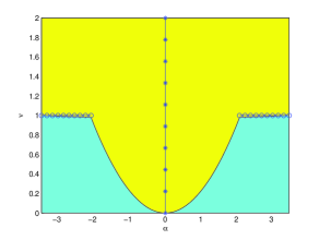
Figure 2: Stability Diagram ($C_{7},C_{8}$)

Here $0\leq\nu\leq 2$ and $\alpha\neq 0.$ The cyan-shaded area ie the area bounded by $\nu=0,\nu=1$ and $\nu=\frac{2\alpha^{2}}{9}$ represents stability. The yellow region represents saddle system (25). The ’o’ marked lines are those parameter values for which the system (25) is center-stable.

IV.9 Critical Point $C_{9}$

In this case, it is necessary that $\alpha\neq 0.$

For this case, $A=\left(\begin{array}[]{c}-\frac{3\nu}{2\alpha}\\ \frac{3\nu}{2\alpha}\\ \frac{2\alpha^{2}-9}{2\alpha^{2}}\\ \end{array}\right).$

The Jacobian matrix of the system (25) at $C_{9}$ has the characteristic polynomial as following :

$$\lambda^{3}+(3\nu-\frac{3}{2})\lambda^{2}+[\frac{18\nu\alpha^{2}-81}{4\alpha^{2}}]\lambda-\frac{27(2\alpha^{2}-9)(\nu-1)}{4\alpha^{2}}=0.$$ (36)

This polynomial has eigenvalues as $3(1-\nu),\frac{-3\alpha+3\sqrt{36-7\alpha^{2}}}{4\alpha}$ and $\frac{-3\alpha-3\sqrt{36-7\alpha^{2}}}{4\alpha}.$ The stability analysis when $\nu\neq 1$ and $\alpha\neq-\frac{3}{\sqrt{2}},\frac{3}{\sqrt{2}}$ (hyperbolic cases) are easy.

Therefore we present a table containing all the non-hyperbolic subcases for $C_{9}$. In the end we will present a diagram in $\alpha-\nu$ plane to show the complete stability analysis as usual.

Table 15: $C_{9}$(Reduced System)

$\nu$	$\alpha$	Center Manifold	Reduced System
$1$	$\frac{3}{\sqrt{2}}$	id to subcase (a) of $C_{7}$	id to subcase (a) of $C_{7}$
$1$	$-\frac{3}{\sqrt{2}}$	id to subcase (b) of $C_{7}$	id to subcase (b) of $C_{7}$
$\neq 1$	$\frac{3}{\sqrt{2}}$	id to subcase (f) of $C_{5}$	id to subcase (f) of $C_{5}$
$\neq 1$	$-\frac{3}{\sqrt{2}}$	id to subcase (h) of $C_{6}$	id to subcase (h) of $C_{6}$
$1$	$\alpha\neq-\frac{3}{\sqrt{2}},\frac{3}{\sqrt{2}}$	$\bar{\bar{y}}=O(\bar{\bar{x}}^{3}),\bar{\bar{\Omega_{m}}}=O(\bar{\bar{x}}^{3})$	$\bar{\bar{x}}^{\prime}=0$

For the last subcase, $P=\left(\begin{array}[]{ccc}0&\frac{\alpha}{6}+\frac{\alpha^{2}(\alpha-\sqrt{36-7\alpha^{2}})}{12(2\alpha^{2}-9)}&\frac{\alpha}{6}+\frac{\alpha^{2}(\alpha+\sqrt{36-7\alpha^{2}})}{12(2\alpha^{2}-9)}\\ 0&-\frac{\alpha}{6}+\frac{\alpha^{2}(\alpha-\sqrt{36-7\alpha^{2}})}{12(2\alpha^{2}-9)}&-\frac{\alpha}{6}+\frac{\alpha^{2}(\alpha+\sqrt{36-7\alpha^{2}})}{12(2\alpha^{2}-9)}\\ 1&1&1\\ \end{array}\right).$

We find again that the stability diagram for $C_{9}$ and $C_{10}$ is totally same. Hence it will be presented at the end of the next subsection of $C_{10}$.

IV.10 Critical Point $C_{10}$

This is the last subcase. In this case too it is necessary that $\alpha\neq 0.$

Also, $A=\left(\begin{array}[]{c}-\frac{3\nu}{2\alpha}\\ \frac{3\nu}{2\alpha}\\ \frac{2\alpha^{2}-9}{2\alpha^{2}}\\ \end{array}\right).$

The Jacobian matrix of the system (25) at $C_{10}$ has the characteristic polynomial

$$\lambda^{3}+(3\nu-\frac{3}{2})\lambda^{2}+[\frac{18\nu\alpha^{2}-81}{4\alpha^{2}}]\lambda+\frac{27(2\alpha^{2}-9)(\nu-1)}{4\alpha^{2}}=0.$$ (37)

which has eigenvalues as $3(1-\nu),\frac{-3\alpha+3\sqrt{36-7\alpha^{2}}}{4\alpha}$ and $\frac{-3\alpha-3\sqrt{36-7\alpha^{2}}}{4\alpha}.$ The stability analysis when $\nu\neq 1$ and $\alpha\neq-\frac{3}{\sqrt{2}},\frac{3}{\sqrt{2}}$ (hyperbolic cases) are easy again.

Therefore we will present a table containing all the non-hyperbolic subcases for this critical point. At the end we will present the stability diagram in $\alpha-\nu$ plane.

Table 16: $C_{10}$(Reduced System)

$\nu$	$\alpha$	Center Manifold	Reduced System
$1$	$\frac{3}{\sqrt{2}}$	id to subcase (a) of $C_{8}$	id to subcase (a) of $C_{8}$
$1$	$-\frac{3}{\sqrt{2}}$	id to subcase (b) of $C_{8}$	id to subcase (b) of $C_{8}$
$\neq 1$	$\frac{3}{\sqrt{2}}$	id to subcase (f) of $C_{6}$	id to subcase (f) of $C_{6}$
$\neq 1$	$-\frac{3}{\sqrt{2}}$	id to subcase (h) of $C_{5}$	id to subcase (h) of $C_{5}$
$1$	$\alpha\neq-\frac{3}{\sqrt{2}},\frac{3}{\sqrt{2}}$	$\bar{\bar{y}}=O(\bar{\bar{x}}^{3}),\bar{\bar{\Omega_{m}}}=O(\bar{\bar{x}}^{3})$	$\bar{\bar{x}}^{\prime}=0$

For the last subcase, $P=\left(\begin{array}[]{ccc}0&\frac{\alpha}{6}+\frac{\alpha^{2}(\alpha-\sqrt{36-7\alpha^{2}})}{12(2\alpha^{2}-9)}&\frac{\alpha}{6}+\frac{\alpha^{2}(\alpha+\sqrt{36-7\alpha^{2}})}{12(2\alpha^{2}-9)}\\ 0&\frac{\alpha}{6}-\frac{\alpha^{2}(\alpha-\sqrt{36-7\alpha^{2}})}{12(2\alpha^{2}-9)}&\frac{\alpha}{6}-\frac{\alpha^{2}(\alpha+\sqrt{36-7\alpha^{2}})}{12(2\alpha^{2}-9)}\\ 1&1&1\\ \end{array}\right).$

Lastly, we provide the stability diagram in the $\alpha-\nu$ plane for $C_{9}$ and $C_{10}$ and end this section :

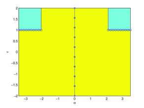
Figure 3: Stability Diagram ($C_{9},C_{10}$)

Here it is necessary that $\alpha\neq 0.$ The two squares in the top corners bounded by the lines $\nu=1,\alpha=\frac{3}{\sqrt{2}}$ and $\nu=1,\alpha=-\frac{3}{\sqrt{2}}$ respectively are cyan-shaded. They represent the parameter values for which the system (25) is stable. The rest of the region represents saddle system.The ’o’ marked line represents center-stability.

At the end of this section, we will present the phase plane diagrams of the autonomous system (25) for various values of the parameter $\nu$ and $\alpha$ in figures (4)-(7) The last diagram (8) depicts the vector fields of the autonomous system (25).

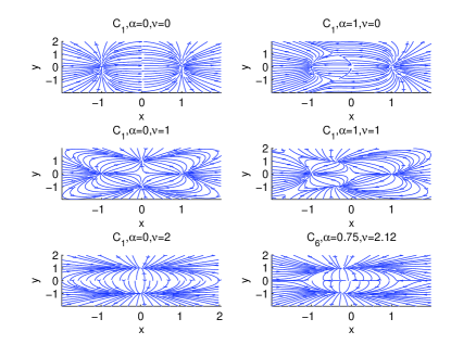
Figure 4: $C_{1},C_{6}$

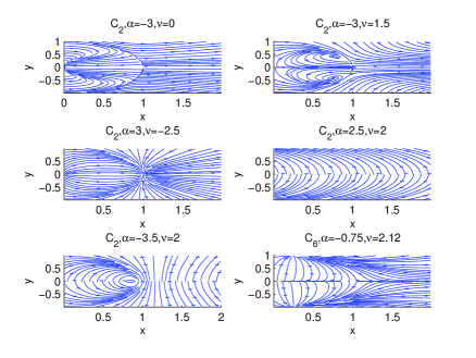
Figure 5: $C_{2},C_{6}$

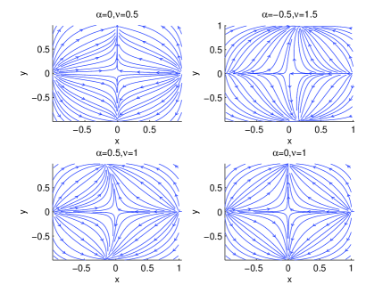
Figure 6: $C_{3}$

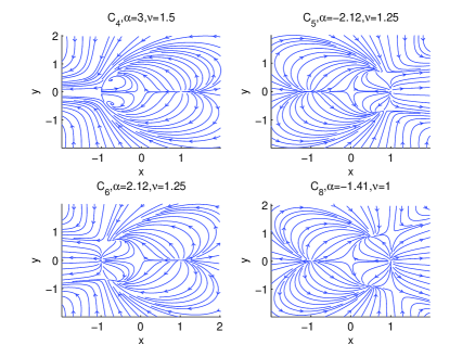
Figure 7: $C_{4},C_{5},C_{6},C_{8}$

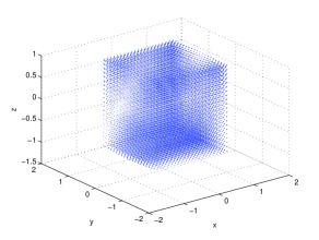
Figure 8: Vector field diagram of (25)

V Cosmological Interpretations and Conclusion

The present work deals with a cosmological model consisting of three non-interacting fluids namely the baryonic matter in the form of perfect fluid ($p_{b}=(\nu-1)\rho_{b}$), dark matter in the form of dust and dark energy as a scalar field respectively. This cosmological model has been studied in the framework of dynamical system analysis by forming the evolution equations (Einstein’s field equations) into an autonomous system with suitable transformation of the variables. In table 1, it has been shown that there are $10$ equilibrium points ($C_{1}$-$C_{10}$) of the autonomous system. The values of the relevant cosmological parameters at the equilibrium points have also been presented in table 2.

The equilibrium point $C_{1}$ is completely dominated by the baryonic matter and as expected in standard cosmology, the model will be in decelerating phase if the baryonic fluid is normal (ie, non-exotic: $\nu>\frac{2}{3}$) and it will be in the accelerating era for exotic nature of the matter (ie, $\nu<\frac{2}{3}$).

The equilibrium points $C_{2}$ and $C_{4}$ have identical nature and both of them are not interesting from the cosmological viewpoint as there is deceleration (of unusual magnitude) when matter is completely dominated by DE. The point $C_{3}$ describes a known result of standard cosmology: In the dust era there is deceleration with the value of the deceleration parameter $\frac{1}{2}.$

The equilibrium point $C_{5}$ and $C_{6}$ correspond to cosmological era dominated by the dark energy(DE). The condition ($\alpha^{2}<3$) restricts the DE to be exotic and there is acceleration. By choosing $\alpha$ appropriately it is possible to match the model with the recent observations.

Both the equilibrium points $C_{7}$ and $C_{8}$ in the phase space have identical cosmological behaviors. For real points in the phase space as well as for realistic baryonic fluid, $\nu$ should be restricted as $0<\nu<2.$ The cosmological model is dominated by both the DE and the baryonic matter. In fact, the cosmic phase described by these phase space points (ie $C_{7}$ and $C_{8}$) has dominance of baryon over DE if $\frac{2}{3}<\nu<2$ and there is deceleration. While if $0<\nu<\frac{2}{3}$ then DE dominates the cosmic evolution and there is acceleration.

The scaling solutions represented by the equilibrium points $C_{9}$ and $C_{10}$ are dominated by both the dark matter (DM) and DE. But they are not of much physical interest as they always correspond to dust era of evolution.

Thus, from the dynamical system analysis, the equilibrium points describe various cosmological eras and some of them are interesting from the cosmological viewpoints with recent observed data. Therefore, one may conclude that from complicated cosmological models one may get cosmological inferences without solving the evolution equations, rather by analyzing with dynamical system approach and the present work is an example of this inference.

VI References

References

- (1) S. J. Perlmutter et al. [Supernova Cosmology Project Collaboration], “Measurements of Omega and Lambda from 42 high redshift supernovae”, Astrophys. J. 517 (2), 565-586(1999).
- (2) A. J. Reiss et al. [Supernova Search Team], “Observational evidence from supernovae for an accelerating universe and a cosmological constant”, Astron. J. 116 (3), 1009-1038(1998).
- (3) W. J. Percival et al. [2dFGRS Collaboration], “The 2dF Galaxy Redshift Survey: The Power spectrum and the matter content of the Universe”, Mon. Not. Roy. Astron. Soc. 327 (4), 1297-1306(2001).
- (4) D. N. Spergel et al. [WMAP Collaboration], ”Three Year Wilkinson Microwave Anisotropy Probe (WMAP) Observations : Implications for Cosmology”, Astrophys. J. Suppl. Ser. 170 (2), 377-408 (2007).
- (5) M. Tegmark et al.,”The Three Dimensional Power Spectrum of Galaxies from the Sloan Digital Sky Survey”, Astrophys. J. 606 (2), 702-740(2004).
- (6) D. J. Eisenstein et al.,Astrophys. J. 148, 175(2003).
- (7) E. Komatsu et al.[WMAP Collaboration], ”FIVE-YEAR WILKINSON MICROWAVE ANISOTROPY PROBE OBSERVATIONS: COSMOLOGICAL INTERPRETATION”, Astrophys. J. Suppl. Ser. 180 (2), 330-376(2009).
- (8) S. Weinberg,”The Cosmological Constant Problem”, Rev. Mod. Phys. 61 (1), 1-23(1989).
- (9) L. Amendola, S. Tsujikawa, ”Dark Energy” : Theory. and Observations”, Cambridge, UK : Cambridge University Press (2010).
- (10) N. Mahata and S. Chakraborty, ”A Dynamical system analysis of three fluid cosmological model”, [arXiv:1512.07017v1[gr-qc]], 22 Dec,2015.
- (11) S. M. Carroll,Liv. Rev. Lett. 4, 1(2001).
- (12) Y. Wang, ”Dark Energy”, Willey-VCH (2010).
- (13) L. Perko, ”Differential Equations and Dynamical Systems”, Springer-Verlag : New York (1991).
- (14) D. K. Arrowsmith and C. M. Place, ”An Introduction to Dynamical Systems”, Cambridge Univ. Press : Cambridge, England (1990).
- (15) S. Wiggins, ”Introduction to Applied Nonlinear Dynamical Systems and Chaos”, ”2nd Edition”, Springer, Berlin (2003).
- (16) P. J. E. Peebles and B. Ratra, ”The cosmological constant and dark energy”, Rev. Mod. Phys. 75(2), 559-606(2003).
- (17) B. Ratra and P. J. E. Peebles, ”Cosmological consequences of a rolling homogeneous scalar field”, Phys. Rev. D. 37 (12), 3406-3427(1988).
- (18) R. R. Caldwell and R. Dave and P. J. Steinherdt, ”Cosmological Imprint of an Energy Component with General Equation of State”, Phys. Rev. Lett. 80(8), 1582-1585(1998).
- (19) C. Armendariz-Picon and V. Mukhanov and P. J. Steinherdt, ”Dynamical Solution to the Problem of a Small Cosmological Constant and Late-Time Cosmic Acceleration”, Phys. Rev. Lett. 85(21), 4438-4441(2000).
- (20) Amartya S. Banerjee, ”An Introduction to Center Manifold Theory”.
- (21) C. Armendariz-Picon and V. Mukhanov and P. J. Steinherdt, ”Essentials of k-essence”, Phys. Rev. D. 63(10), 103510(2001).
- (22) R. R. Caldwell and M. Kamionkowski and N. N. Weinberg, ”Causes a Cosmic Doomsday”, Phys. Rev. Lett. 91(7), 071301(2003).
- (23) A. Sen,J. H. E. P 207, 65(2002).
- (24) E. J. Copeland and M. Sami and S. Tsujikawa, ”DYNAMICS OF DARK ENERGY”, Int. J. Mod. Phys. D 15(11), 1753-1935(2006).
- (25) M. Tsamparlis and A. Paliathanasis,”Three-fluid cosmological model using Lie and Noether symmetries”, Class. Quantum Gravity. 29(1), 015006(2012).
- (26) E. J. Copeland and A. R. Riddle and D. Wands, ”Exponential potentials and cosmological scaling solutions.”, Phys. Rev. D. 57(8), 4686-4690(1998).