Geodesics of the hyperbolically symmetric black hole

Abstract

We carry out a systematic study on the motion of test particles in the region inner to the horizon of a hyperbolically symmetric black hole. The geodesic equations are written and analyzed in detail. The obtained results are contrasted with the corresponding results obtained for the spherically symmetric case. It is found that test particles experience a repulsive force within the horizon, which prevents them to reach the center. These results are obtained for radially moving particles as well as for particles moving in the $\theta-R$ subspace. To complement our study we calculate the precession of a gyroscope moving along a circular path (non–geodesic) within the horizon. We obtain that the precession of the gyroscope is retrograde in the rotating frame, unlike the precession close to the horizon ($R=2m+\epsilon$) in the Schwarzschild spacetime, which is forward.

I Introduction

In a recent paper 1 a global description of the Schwarzschild black hole was proposed, which sharply differs from the “classical” picture of the spherically symmetric black hole. The motivation for this proposal was based on the well known fact that any transformation that maintains the static form of the Schwarzschild metric (in the whole space–time) is unable to remove the singularity in the line element rosen . In other words, any coordinate transformation allowing the manifold to extend over the whole space–time (including the region inner to the horizon), necessarily implies that the metric is non-static within the horizon (see for example eddington ; 1b ; fin ; krus ; is ). A simple way to arrive at this conclusion consists in noticing that the Schwarzschild horizon is also a Killing horizon, implying that the time–like Killing vector outside the horizon becomes space–like inside it. If we recall that a static observer is one whose four–velocity is proportional to the Killing time–like vector Caroll , it follows that no static observers can be defined inside the horizon. Further discussion on this point may be found in Rin .

Then, based on the physical point of view that any equilibrium final state of a physical process should be static, the existence of a static solution would be expected over the whole space–time. To achieve that, the following scheme was proposed in 1 .

Outside the horizon ($R>2m$), one has the usual Schwarzschild line element corresponding to the spherically symmetric vacuum solution to Einstein equations, which can be written in polar coordinates in the form

$$ds^{2} = -\left(1-\frac{2m}{R}\right)dt^{2}+\frac{dR^{2}}{\left(1-\frac{2m}{R}\right)}+R^{2}d\Omega^{2},$$

$$d\Omega^{2} = d\theta^{2}+\sin^{2}\theta d\phi^{2}.$$ (1)

As is well known, this metric is static and spherically symmetric, meaning that it admits four Killing vectors:

$$\mathbf{\chi}_{(\mathbf{0})}=\partial_{\mathbf{t}},\quad{\bf\chi_{(2)}}=-\cos\phi\partial_{\theta}+\cot\theta\sin\phi\partial_{\phi}$$

$${\bf\chi_{(1)}}=\partial_{\phi}\quad{\bf\chi_{(3)}}=\sin\phi\partial_{\theta}+\cot\theta\cos\phi\partial_{\phi}.$$ (2)

However, when $R<2m$ the signature changes from (-, +, +, +) to (+, -, +, +) and an apparent line element singularity appears at $R=2m$. Of course, as is also well known, these drawbacks can be removed by coordinate transformations, but at the price that, as mentioned before, the staticity is lost within the horizon.

In order to save the staticity inside the horizon, the model proposed in 1 describes the space time as consisting of a complete four dimensional manifold (described by (1)) on the exterior side and a second complete four dimensional solution in the interior. Additionally a change in signature, as well as a change in the symmetry at the horizon was required. The $\theta-\phi$ sub-manifolds have a spherical symmetry on the exterior and hyperbolic symmetry in the interior. The two meet only at $R=2m$, $\theta=0$.

Thus the model permits for a change in symmetry, from spherical outside the horizon to hyperbolic inside the horizon. Doing so, one has a static solution everywhere, but the symmetry of the $R=2m$ surface is different at both sides of it. We have to stress that we do not know if there is any specific mechanism behind such a change of symmetry and signature. However, the main point is that the change of symmetry (and signature) was the only way we have found to obtain a globally static solution.

Thus, the solution proposed for $R<2m$ is:

$$ds^{2} = \left(\frac{2m}{R}-1\right)dt^{2}-\frac{dR^{2}}{\left(\frac{2m}{R}-1\right)}-R^{2}d\Omega^{2},$$

$$d\Omega^{2} = d\theta^{2}+\sinh^{2}\theta d\phi^{2}.$$ (3)

This is a static solution with the $(\theta,\phi)$ space describing a positive Gaussian curvature.

Besides the time–like Killing vector $\mathbf{\chi}_{(\mathbf{0})}=\partial_{\mathbf{t}}$, it admits three additional Killing vectors which are:

$${\bf\chi_{(1)}} = \partial_{\phi},\qquad{\bf\chi_{(2)}}=-\cos\phi\partial_{\theta}+\coth\theta\sin\phi\partial_{\phi},$$

$${\bf\chi_{(3)}} = \sin\phi\partial_{\theta}+\coth\theta\cos\phi\partial_{\phi}.$$ (4)

A solution to the Einstein equations of the form given by (3), defined by the hyperbolic symmetry (4), was first considered by Harrison Ha , and has been more recently the subject of research in different contexts (see ellis ; 1n ; Ga ; Ri ; Ka ; Ma ; ren and references therein).

In 1 , a general study of radial geodesic at $\theta=0$ was presented, leading to some interesting conclusions about the behaviour of a test particle in this new picture of the Schwarzschild black hole. Our purpose in this work is to carry out a complete study on the geodesics in the region inner to the horizon. Furthermore, some erroneous conclusions about the motion of test particles along the $\theta=0$ axis presented in 1 , will be corrected.

As we shall see here, very important differences appear in the behaviour of test particles inside the horizon, when this region is described by (3), as compared with the results obtained for the “classical” black hole picture. Particularly relevant are the facts that a repulsive acceleration is experienced by the test particle inside the horizon, and that test particles can cross the horizon outwardly, but only along the axis $\theta=0$.

II The Geodesics

The equations governing the geodesics may be derived from the Lagrangian

$$2{\cal L}=g_{\alpha\beta}\dot{x}^{\alpha}\dot{x}^{\beta},$$ (5)

where the dot denotes differentiation with respect to an affine parameter $s$, which for timelike geodesics coincides with the proper time. Then, the Euler-Lagrange equations,

$$\frac{d}{ds}\left(\frac{\partial{\cal L}}{\partial\dot{x}^{\alpha}}\right)-\frac{\partial{\cal L}}{\partial x^{\alpha}}=0,$$ (6)

lead to the geodesic equations, which may also be written in its usual form,

$$\ddot{x}^{\alpha}+\Gamma^{\alpha}_{\beta\gamma}\dot{x}^{\beta}\dot{x}^{\gamma}=0.$$ (7)

Although the general characteristics of geodesics for $R>2m$ are very well known, here we include a very brief resume, in order to contrast these with the results that we shall obtain for $R<2m$.

II.1 Geodesics for $R>2m$ (Schwarzschild)

For the metric (1) the geodesic equations (6) are,

$$\ddot{t}+\frac{2m\dot{t}\dot{R}}{R^{2}(1-\frac{2m}{R})}=0$$ (8)

$$\frac{\ddot{R}}{1-\frac{2m}{R}}-\frac{\dot{R}^{2}m}{R^{2}(1-\frac{2m}{R})^{2}}+\frac{m\dot{t}^{2}}{R^{2}}-R\dot{\theta}^{2}-R\dot{\phi}^{2}\sin^{2}\theta=0,$$ (9)

$$\ddot{\theta}R^{2}+2R\dot{R}\dot{\theta}-R^{2}\dot{\phi}^{2}\sin\theta\cos\theta=0,$$ (10)

$$\ddot{\phi}\sin^{2}\theta+\frac{2\dot{R}\dot{\phi}\sin^{2}\theta}{R}+2\dot{\phi}\dot{\theta}\sin\theta\cos\theta=0.$$ (11)

As is well known, there are unbounded orbits as well as bounded ones. In this latter case we have elliptic orbits with a perihelion shift. There are also circular orbits, which may be stable or unstable.

Let us first consider circular geodesics ($\dot{R}=\dot{\theta}=0$), then it follows from (8) and (11) that $\ddot{t}=\ddot{\phi}=0$, and from (10) we obtain

$$R^{2}\dot{\phi}^{2}\sin\theta\cos\theta=0,$$ (12)

which implies that circular geodesics do exist on the plane $\theta=\pi/2$. Of course, due to the spherical symmetry, if the particle is not on this plane we can always rotate coordinates until it is. Accordingly without loss of generality we may choose $\theta=\pi/2$.

Next, from (9) we obtain

$$\frac{m\dot{t}^{2}}{R^{2}}-R\dot{\phi}^{2}=0,$$ (13)

then defining the angular velocity as $\omega=\frac{\dot{\phi}}{\dot{t}}$ we obtain the Kepler law

$$\omega^{2}=\frac{m}{R^{3}}.$$ (14)

Let us now define a “velocity” by An :

$$W^{i}=\frac{dx^{i}}{\sqrt{-g_{00}}dx^{0}},$$ (15)

with

$$dx^{i}=(0,dx^{1},dx^{2},dx^{3}).$$ (16)

Then for the tangential velocity of a circular orbit we find

$$W^{2}\equiv|W^{i}W_{i}|=\omega^{2}R^{2}\left(1-\frac{2m}{R}\right)^{-1}.$$ (17)

In the weak field limit $m/R<<1$ we recover the classical expression $W=\omega R$. The geodesics are null, timelike or spacelike if $W=1,<1,>1$ respectively.

Let us now focus on the radial motion of test particles. First of all, notice that as a consequence of the symmetry (spherical and time–independence) we have three constants of motion which are energy and angular momentum (magnitude and direction), defined respectively by, (on the plane $\theta=\pi/2$),

$$\frac{\partial{\cal L}}{\partial\dot{t}}=constant\equiv E=-\dot{t}\left(1-\frac{2m}{R}\right),$$ (18)

$$\frac{\partial{\cal L}}{\partial\dot{\phi}}=constant\equiv L=\dot{\phi}R^{2},$$ (19)

$$\frac{\partial{\cal L}}{\partial\dot{\theta}}=constant\equiv P_{\theta}=\dot{\theta}R^{2}.$$ (20)

Then the first integral of (9) may be written as

$$\dot{R}^{2}=E^{2}-V^{2},$$ (21)

with

$$V^{2}=\left(1-\frac{2}{y}\right)\left(\frac{\tilde{L}^{2}}{y^{2}}+1\right)$$ (22)

where $y\equiv R/m$,    $\tilde{L}^{2}\equiv\frac{L^{2}}{m^{2}}$.

The above equation is the same equation (10) in 1 . However in this reference it was used to study the motion inside the horizon, which obviously is incorrect (the potential $V$ given by (22) is correct but valid only outside the horizon).

For the motion along the axis $\theta=0$ we have $L=0$, then for the value of energy given in Figure 1, all possible radial geodesics (for $R>2m$) extend between the horizon (the vertical line) and the value of $y$ where the horizontal line crosses the curve $V^{2}$ as given by (22). We shall discuss about the behaviour of the particle for $R<2m$ in the next subsection. For larger values of $E$, such that $E>V$, unbounded trajectories are allowed.

For $\theta=\pi/2$ and the values of energy $E$ and the angular momentum $\tilde{L}$ given in Figure 2, the horizontal line crosses the curve $V^{2}$ as given by (22) (for $R>2m$) at two points, say $y_{1},y_{2}$ ($y_{2}>y_{1}$). Thus there are radial geodesics, outside the horizon, in the interval $y_{1}>y>2$, and unbounded trajectories for $y>y_{2}$. The unstable circular geodesic corresponds to the value of $E=E_{c}$. The region inner to the horizon shall be considered in the next subsection.

All the results above are well known, and apply for $R>2m$.

II.2 Geodesics for the hyperbolically symmetric black hole ($R<2m$)

Let us now analyze the geodesic structure for the region within the horizon, where we assume the space–time to be described by the hyperbolically symmetric solution (3).

Using (3) we obtain from (6) or (7):

$$\ddot{t}-\frac{2m\dot{t}\dot{R}}{R^{2}\left(\frac{2m}{R}-1\right)}=0,$$ (23)

$$\ddot{R} + \frac{\dot{R}^{2}m}{R^{2}(\frac{2m}{R}-1)}-\frac{m\dot{t}^{2}(\frac{2m}{R}-1)}{R^{2}}$$ (24)

$$- R\dot{\theta}^{2}\left(\frac{2m}{R}-1\right)-R\dot{\phi}^{2}\sinh^{2}\theta\left(\frac{2m}{R}-1\right)=0,$$

$$\ddot{\theta}R^{2}+2R\dot{R}\dot{\theta}-R^{2}\dot{\phi}^{2}\sinh\theta\cosh\theta=0,$$ (25)

$$\ddot{\phi}+\frac{2\dot{R}\dot{\phi}}{R}+2\dot{\phi}\dot{\theta}\coth\theta=0.$$ (26)

Let us first consider circular geodesics along the $\phi$ direction. Thus $\dot{R}=\dot{\theta}=0$, and it follows from (25)

$$R^{2}\dot{\phi}^{2}\sinh\theta\cosh\theta=0,$$ (27)

from which we can see that, unlike the case $R>2m$, there are not circular geodesics in the $\phi$ direction, not even unstable ones.

Furthermore, from (24) it follows that

$$\frac{m\dot{t}^{2}}{R^{2}}+R\dot{\phi}^{2}\sinh^{2}\theta=0,\Rightarrow\omega^{2}=-\frac{m}{R^{3}\sinh^{2}\theta}$$ (28)

which is clearly unacceptable, and confirms the conclusion above.

Let us now consider geodesics along the $\theta$ direction, i.e. $\dot{R}=\dot{\phi}=0$, then it follows from (24)

$$\frac{m\dot{t}^{2}}{R^{2}}+R\dot{\theta}^{2}=0,\Rightarrow\frac{\dot{\theta}^{2}}{\dot{t}^{2}}=-\frac{m}{R^{3}},$$ (29)

implying that there are not geodesics exclusively along the $\theta$ direction.

More generally if we assume $\dot{R}=0$ then it follows from (24)

$$\frac{m\dot{t}^{2}}{R^{2}}+R\dot{\theta}^{2}+R\dot{\phi}^{2}\sinh^{2}\theta=0,$$ (30)

implying that no motion is possible unless $\dot{R}\neq 0$.

If we assume that $\dot{\phi}=0$ then it follows at once from (25) that

$$\dot{\theta}R^{2}=constant\Rightarrow P_{\theta}=constant,$$ (31)

whereas, if we assume $\dot{\theta}=0$, then it follows from (25) that $\dot{\phi}=0$.

Next, let us assume that at some given initial $s=s_{0}$ we have $\dot{\theta}=0$, then it follows at once from (25) that such a condition will propagate in time only if $\theta=0$ or $\dot{\phi}=0$. In other words, any $\theta=constant$ trajectory is unstable except $\theta=0$, unless $\dot{\phi}=0$. It is worth stressing the difference between this case and the situation in the $R>2m$ region (see (10)).

Thus only the following cases are allowed:

1. Purely radial geodesics $\dot{R}\neq 0$, $\dot{\theta}=\dot{\phi}=0$.

2. Geodesics in the $R,\theta$ plane (i.e. $\dot{\phi}=0,\dot{R},\dot{\theta}\neq 0$)

3. The general case $\dot{R},\dot{\theta},\dot{\phi}\neq 0$.

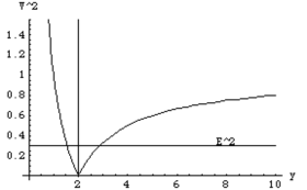
Figure 1: $V^{2}$ as function of $y$ for $\theta=0$. The vertical line is the horizon. The horizontal line corresponds to the value of $E^{2}=.315$

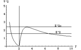
Figure 2: $V^{2}$ as function of $y$ for $\theta=\pi/2$, and $\tilde{L}^{2}=55$. The vertical line is the horizon. The lower horizontal line corresponds to the value of $E^{2}=1.71$. The higher horizontal line corresponds to the value of $E^{2}_{c}=2.42$

Let us first consider the radial motion of test particles inside the horizon. As, for the region exterior to the horizon, we have two constants of motions which are energy and angular momentum, defined respectively by

$$\frac{\partial{\cal L}}{\partial\dot{t}}=constant\equiv E=\dot{t}\left(\frac{2m}{R}-1\right),$$ (32)

$$\frac{\partial{\cal L}}{\partial\dot{\phi}}=constant\equiv L=-\dot{\phi}R^{2}\sinh^{2}\theta,$$ (33)

however, the canonical momentum $P_{\theta}$ now is not conserved, unless $\dot{\phi}=0$,

$$\frac{\partial{\cal L}}{\partial\dot{\theta}}\equiv P_{\theta}=-\dot{\theta}R^{2}.$$ (34)

For the radial motion along the symmetry axis $\theta=0$, both $L$ and $P_{\theta}$ vanish. Also, as mentioned before, if we assume that at some initial time $\dot{\theta}=0$, then the trajectory along the $\theta=0$ axis will be stable in time.

Then, the first integral of (24) with $\dot{\phi}=\dot{\theta}=0$ reads ,

$$\dot{R}^{2}=E^{2}-V^{2},$$ (35)

with

$$V^{2}=\left(\frac{2}{y}-1\right),$$ (36)

where $y\equiv R/m$.

The above equation is the same equation (15) in 1 . However in this latter reference it was used to study the motion outside the horizon, which obviously is incorrect. Again, the potential $V$ given by (36 is correct but valid only inside the horizon.

As we see from Figure 1, for the given value of $E$, the test particle inside the horizon never reaches the center, moving between the point where the horizontal line crosses $V^{2}$ (as given by (36)) and the horizon. In principle the particle may cross the horizon and bounces back at the point (outside the horizon) where the horizontal line crosse $V^{2}$ (as given by (22).

Thus for this particular value of energy we have a bounded trajectory with extreme points at both sides of the horizon. For sufficiently large (but finite) values of energy, the particle moves between a point close to, but at finite distance from the center and $R\rightarrow\infty$.

Two main conclusions emerge at this point, for the test particle moving under the conditions stated above:

1. The particle never reaches the center, approaching it asymptotically as $E\rightarrow\infty$.

2. The particle may cross the horizon, not only inwardly but also outwardly.

The sharp difference between this behaviour of the test particle inside the horizon, and the corresponding behaviour in the “classical” picture of the Schwarzschild black hole, does not need to be further emphasized.

Let us now consider the radial motion on the $\theta=\pi/2$ plane. First of all we observe that, as mentioned before, if we want to remain on that plane, inside the horizon, we must have $\dot{\phi}=L=0$, and the situation is very similar to the case $\theta=0$, with one important difference; now the trajectory is unstable against perturbations of the angular momentum, and we should expect the particle to leave the $\theta=\pi/2$ plane. Nevertheless, for sake of completeness we have also plotted this case in figure 2.

Three main differences between this case and the situation for $R>2m$, deserve to be emphasized.

1. For $R>2m$ the motion on the plane $\theta=constant\neq 0$ is stable.

2. for $R<2m$ the motion on the plane $\theta=constant\neq 0$ requires $L=0$.

3. Even if $L=0$, for $R<2m$, the trajectory will be unstable against perturbations of the angular momentum.

These conclusions are qualitatively the same for any $\theta=constant\neq 0$.

The results exhibited above show that the motion along the $\theta=0$ axis is sharply different from other trajectories. More specifically, the instabilities of the motion for any $\theta=constant\neq 0$ trajectory, implies that, unless the particle moves along $\theta=0$, all trajectories must involve variations of $\theta$. Therefore, we shall next find the trajectories of test particles on the plane $R-\theta$ for any $\phi=constant$, in which case the momentum $P_{\theta}$ is constant and $L=0$. It is worth noticing that due to axial symmetry, the motion on any two dimensional slice $\phi=constant$ is invariant with respect to rotations around the symmetry axis. Therefore the restricted case $L=0$ provides the most relevant physical information about the motion of the particle without integrating the full system of geodesic equations.

Then, the first integral of (24) becomes

$$\dot{R}=\sqrt{E^{2}-\left(\frac{2m}{R}-1\right)\left(\frac{P^{2}_{\theta}}{R^{2}}+1\right)}.$$ (37)

Since we are interested in the spatial trajectories, we use

$$\dot{R}=-\frac{P_{\theta}}{R^{2}}R^{\prime},\qquad R^{\prime}=\frac{dR}{d\theta},$$

to write (37) as

$$z^{\prime}=\frac{1}{k}\sqrt{E^{2}-(z-1)(k^{2}z^{2}+1)}$$ (38)

where. $z=\frac{2m}{R}$, and $k=\frac{P_{\theta}}{2m}$, thus $z$ changes in the domain $(-\infty,1]$. We have integrated the equation above for a wide range of values of the parameters $k,E$. The integration was carried out with the boundary condition that all trajectories coincide at $\theta=0$, $z=1$.

Two main results emerge from all these models. On the one hand we found that the test particle never crosses the horizon outwardly, approaching it as $k$ tends to zero, as expected from Figures 1,2. To illustrate this point we show the results of the numerical integration of (38) for the values indicated in the legends of Figures 3, 4, however this conclusion holds for all possible trajectories with finite values of $E$ and $k$. In these figures the axes cross at the origin (the center of symmetry) and the length of a line segment from the center to any point on the curve is given by $z$ and the angle of this line with the horizontal axis is $\theta$. On the other hand, we found that the test particle never reaches the center, approaching it asymptotically as $k,E\rightarrow\infty$.

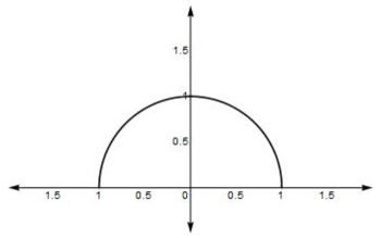
Figure 3: The trajectory of the test particle in the sub–space $R-\theta$, for $k=\frac{1}{10000}$ and $E=3$.

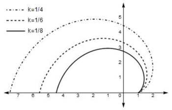
Figure 4: The trajectory of the test particle in the sub–space $R-\theta$ for three values of $k$, ($1/4,1/6,1/8$) and $E=3$.

In order to understand the results above, it is convenient to calculate the four–acceleration of a static observer in the frame of (3). We recall that a static observer is one whose four velocity $U^{\mu}$ is proportional to the Killing time–like vector Caroll , i.e.

$$U^{\mu}=\left(\frac{1}{\sqrt{\frac{2m}{R}-1}},0,0,0\right).$$ (39)

Then for the four–acceleration $a^{\mu}\equiv U^{\beta}U^{\mu}_{;\beta}$ we obtain for the region inner to the horizon

$$a^{\mu}=\left(0,-\frac{m}{R^{2}},0,0\right),$$ (40)

whereas for the outer region described by (1) we obtain

$$a^{\mu}=\left(0,\frac{m}{R^{2}},0,0\right).$$ (41)

The physical meaning of (41) is clear, it represents the inertial radial acceleration outwardly directed, which is necessary in order to maintain static the frame, by canceling the gravitational acceleration exerted on the frame. Since the former is directed radially outwardly, it means that the gravitational force is attractive, as expected. However, inside the horizon the four–acceleration as defined by (40) is directed inwardly, implying that a repulsive force is acting on the particle in that region. This remarkable fact explains the peculiarities of the orbits inside the horizon.

The above discussion may be presented in an alternative format (see H for details). Let us introduce a locally defined coordinate system ($T,X,\theta,\phi)$ associated with a locally Minkowskian observer or, equivalently, a tetrad field associated with this Minkowskian observer, i.e.

$$dX=\sqrt{-g_{RR}}dR\qquad dT=\sqrt{g_{tt}}dt$$ (42)

then for a particle instantaneously at rest inside the horizon, we have:

$$\frac{d^{2}X}{dT^{2}}=\frac{m}{R^{2}\sqrt{(\frac{2m}{R}-1)}},$$ (43)

where (3) and (24) have been used. From the above equation, the repulsion experimented by the particle is clearly established.

For the Schwarzschild solution (1) for $R>2m$, the corresponding expression reads:

$$\frac{d^{2}X}{dT^{2}}=-\frac{m}{R^{2}\sqrt{(1-\frac{2m}{R})}},$$ (44)

indicating the attractive nature of the gravitation force in that region.

III Gyroscope precession of a gyroscope along a circular, non–geodesic path

We shall now calculate the precession of a gyroscope moving along a circular trajectory inside the horizon. Since, as we have already mentioned, no circular geodesics exist in that region, the trajectory of the gyroscope cannot be a geodesic. This calculation can be performed in different ways, here we shall use the Rindler-Perlick method Rindler , which we find particularly suitable for our purpose.

This method consists in transforming the angular coordinate $\phi$ by

$$\phi=\phi^{\prime}+\omega t,$$ (45)

where $\omega$ is a constant. Then the original frame is replaced by a rotating frame. The transformed metric is written in a canonical form,

$$ds^{2}=-e^{2\Psi}(dt-\omega_{i}dx^{i})^{2}+h_{ij}dx^{i}dx^{j},$$ (46)

with latin indexes running from 1 to 3 and $\Psi,\omega_{i}$ and $h_{ij}$ depending on the spatial coordinate $x^{i}$ only (we are omitting primes). Then, it may be shown that the rotation three vector $\Omega^{i}$ of the congruence of world lines $x^{i}=$constant is given by Rindler ,

$$\Omega^{i}=\frac{1}{2}e^{\Psi}(\det h_{mn})^{-1/2}\epsilon^{ijk}\omega_{k,j},$$ (47)

where the comma denotes partial derivative, and the three vector ${\mathbb{\Omega}}$ is related to the vorticity tensor $\omega_{\alpha\beta}$ by

$$\omega_{kj}=\Omega^{l}\eta_{lkj},$$ (48)

where $\eta_{lkj}$=$(deth_{mn})^{1/2}\epsilon_{ikj}$ is the Levi–Civita tensor associated to the spatial metric $h_{mn}$.

It is clear from the above that, since $\Omega^{i}$ describes the rate of rotation with respect to the proper time at any point at rest in the rotating frame, relative to the local compass of inertia, then $-\Omega^{i}$ describes the rotation of the compass of inertia (the gyroscope) with respect to the rotating frame.

Thus let us consider a gyroscope moving around the center along a circular orbit (non–geodesic), and let us calculate its precession. Since $-{\mathbb{\Omega}}$ describes the precession of the gyroscope relative to the lattice, then after one revolution the orientation of the gyroscope, in the rotating frame, changes by

$$\Delta\phi^{\prime}=-\Omega e^{\Psi}\Delta t.$$ (49)

Obviously, the precession per revolution relative to the original system is:

$$\Delta\phi=\Delta\phi^{\prime}+2\pi.$$ (50)

The case of the Schwarzschild metric ($R>2m$) has been calculated in Rindler for the $\theta=\pi/2$ plane. They obtain for the magnitude of the vorticity ${\mathbb{\Omega}}$ (notice that a $\omega$ is missing in the equation (38) in Rindler ):

$$\Omega=\frac{\omega\left(1-\frac{3m}{R}\right)}{1-\frac{2m}{R}-R^{2}\omega^{2}},$$ (51)

and for the total precession $\Delta\phi$

$$\Delta\phi=-2\pi\left[\frac{\left(1-\frac{3m}{R}\right)}{\sqrt{1-\frac{2m}{R}-R^{2}\omega^{2}}}-1\right].$$ (52)

From the expressions above, we see that at $R=3m$ the orientation of the gyroscope is locked to the lattice ($\Omega=0$). In the region between the horizon and $R=3m$, if $\omega$ is sufficiently small so that the orbits are time–like, $\Omega$ becomes negative and the precession of the gyroscope is forward even in the rotating frame ($\Delta\phi^{\prime}>0$). Thus the total precession $\Delta\phi$ exceeds $2\pi$.

However for the region interior to the horizon, as described by (3) the situation is completely different. Indeed, retracing the same steps leading to (51) and (52) we obtain (for the plane $\theta=\pi/2$)

$$\Omega=\frac{\omega\alpha\left(\frac{3m}{R}-1\right)}{\frac{2m}{R}-1-R^{2}\omega^{2}\alpha^{2}},$$ (53)

$$\Delta\phi^{\prime}=-\frac{2\pi\alpha\left(\frac{3m}{R}-1\right)}{\sqrt{\frac{2m}{R}-1-R^{2}\omega^{2}\alpha^{2}}},$$ (54)

$$\Delta\phi=-2\pi\left[\frac{\alpha\left(\frac{3m}{R}-1\right)}{\sqrt{\frac{2m}{R}-1-R^{2}\omega^{2}\alpha^{2}}}-1\right],$$ (55)

where $\alpha\equiv\sinh({\pi/2})$.

As it is apparent from (54), for sufficiently small $\omega$, so that the orbits are time–like, in the region inner to the horizon described by the metric (3), the precession of the gyroscope is retrograde in the rotating frame. Obviously the total precession in the original frame is now smaller than $2\pi$, as it happens for the Thomas precession in Minkowski space–time (see eqs. (32, 33) in Rindler ).

IV Conclusions

In the classical picture of the Schwarzschild black hole, any particle inside the horizon is bound to reach the center in a finite proper time interval. This is the basic fact behind the “classical” black hole paradigm. However, as we have seen here, if we adopt the point of view proposed in 1 , we find that the kinematic and dynamic properties of a test particle inside the horizon, are quite different. Indeed, not only are the test particles not condemned to displace to the center, but they cannot reach the center for any finite value of energy as shown in figures (1, 2, 4). This fact is brought about by the existence of a repulsive force within the horizon, that pushes the test particle away from the center.

Besides the feature commented above, there is another important difference with respect to the “classical” picture. It consists in the fact that the particles inside the horizon may in principle leave that region along the axis $\theta=0$. Thus, the particle may come from $R\rightarrow\infty$ crosses the horizon, bounces back before reaching the center and crosses the horizon outward. As we have seen this can be done only along this axis, all other trajectories, as illustrated by figures (2, 3), never cross the horizon. This point was already emphasized in 1 , although it must be stressed that other conclusions, concerning the motion of test particles presented in 1 are erroneous due to an incorrect use of equations (34) and (35). Also, it is worth noticing that it is possible that a quantum theory would permit a particle to tunnel across the horizon for $\theta\neq 0$.

Finally we have seen that the precession of a gyroscope moving along a circle inside the horizon is retrograde, whereas, close to the horizon, but at the outside of it ($R=2m+\epsilon$, where $\epsilon<<2m$ and positive), the precession is forward.

Before closing this section we would like to raise two questions, and to speculate about their possible answers.

1. What is the physical origin of the repulsion experienced by the test particle inside the horizon?

2. What could be the observational consequences of the fact that the test particle could leave the horizon along the $\theta=0$ axis.?

With respect to the first question, let us mention that repulsive forces in the context of general relativity have been reported before, in many different scenarios, (see repulsive3 ; papapetrou ; repulsive2 ; repulsive4 ; re1 ; repulsive5 ; H ; maluf ; s1 ). However, neither of these references provides a satisfactory physical explanation about the origin of such an effect. Although this requires a deep and careful analysis, which is beyond the scope of this manuscript, we speculate that the repulsion might be related to quantum vacuum of the gravitational field.

With respect to the second question, we speculate that the hyperbolically symmetric black hole might be invoked to explain extragalactic relativistic jets.

Indeed, relativistic jets are highly energetic phenomena which have been observed in many systems (see Margon ; Sams and references therein), usually associated with the presence of a compact object, and exhibiting a high degree of collimation. The spin and the magnetic field of a compact object are some of the many mechanisms proposed so far to explain this phenomenon Blandford . However, no consensus has been reached until now, concerning the basic mechanism for its origin. Still worse, the basic physical ideas underlying the occurrence of these jets are hidden by the great number of models available (see Blandford ; B1 ; B2 ; M1 ; m2 ; s2 and references therein) and their complexity, implying a large number of assumptions. Under these circumstances, we speculate that the possible ejection, and collimation, of test particles along the $\theta=0$ axis, produced by the repulsive force acting within the horizon, could be considered as a possible engine behind the jets.

To summarize: Even though our proposal for the region inside the horizon is highly “heterodox”, the results ensuing from its adoption lead to specific observational consequences and provide possible explanation to some so far unresolved astrophysical quandaries. It goes without saying that the final word about the physical viability of the hyperbolically symmetric black hole belongs to the observational evidence. Nevertheless, in the light of the results here presented we believe that until such evidence is provided, our proposal is significant enough as to consider it further.

- (1) L. Herrera and L. Witten, Adv. High En. Phys. 2018, 3839103, (2018).
- (2) N. Rosen, The nature of Schwarzschild singularity in “Relativity” Proceedings of the Relativity Conference in the Midwest, M. Carmeli, S. I. Fickler and L. Witten, Eds. (Plenum Press, New York, 1970).
- (3) A. S. Eddington, Nature 113, 192 (1924).
- (4) G. Lemaître, Ann. Soc. Sci. Bruxelles A 53, 51 (1933).
- (5) D. Finkelstein, Phys. Rev. 110, 965 (1958).
- (6) M. D. Kruskal, Phys. Rev. 119, 1743 (1960).
- (7) W. Israel, Phys. Rev. 143, 1016 (1966).
- (8) S. Caroll, Spacetime and Geometry. An Introduction to General Relativity (Addison Wesley, San Francisco 2004), p.246.
- (9) W. Rindler, Relativity. Special, General and Cosmological (Oxford University Press, New York, 2001), p. 260, 261.
- (10) B. K. Harrison, Phys. Rev. 116, 1285 (1959).
- (11) G. Ellis, J. Math. Phys. 8, 1171 (1967).
- (12) H. Stephani, D. Kramer, M. MacCallum, C. Honselaers, and E. Herlt, Exact Solutions to Einstein’s Field Equations (Cambridge University Press, Cambridge, England), (2003), 2nd Ed.
- (13) M. Gaudin, V. Gorini, A. Kamenshchik, U. Moschella and V. Pasquier, Int. J. Mod. Phys. D 15,1387 (2006).
- (14) L. Rizzi, S. L. Cacciatori, V. Gorini, A. Kamenshchik, and O. F. Piattella, Phys. Rev. D 82, 027301 (2010).
- (15) A. Yu. Kamenshchik, E. O. Pozdeeva, A. A. Starobinsky, A. Tronconi, T. Vardanyan, G. Venturi and S. Yu. Verno, Phys. Rev. D 98, 124028 (2018).
- (16) T. Madler, Phys. Rev. D 99, 104048,(2019).
- (17) J. Ren, arXiv:1910.06344v1 [hep-th].
- (18) J. L. Anderson, Principles of Relativity ( Academic Press, New York 1967) Sec. 10.6(a)
- (19) L. Herrera, Found. Phys. Lett. 18, 21 (2005).
- (20) W. Rindler and V. Perlick, Gen. Rel. Grav. 22, 1067 (1990).
- (21) E. L. Schuking, Atti del Convegno sulla Cosmologia (G Barbera Editor, Italy, Florence,1966).
- (22) A. Papapetrou Lectures on General Relativity (D. Reidel, Dordrecht-Holland, 1974).
- (23) W. B. Bonnor,J. Phys. A10, 1673 (1977).
- (24) L. Herrera and N. O. Santos J. Math. Phys. 39, 3817 (1998).
- (25) C. Barbachoux, J. Gariel, G. Marcilhacy and N. O. Santos, Int.J.Modern Phys.D 11, 1255 (2002).
- (26) W. B. Bonnor, Class. Quantum Grav. 19, 146 (2002).
- (27) J. W. Maluf, Gen. Relativ. Gravit. 46, 1734 (2014).
- (28) J. Gariel, N. O. Santos, A. Wang, Gen. Relativ. Gravit. 48, 66 (2016).
- (29) B. A. Margon, Annu. Rev. Astr. Astrophys 22 507(1984);.
- (30) B. J. Sams, B .J. A. Eckart and R. Suyaev, Nature 382 47(1996).
- (31) R D Bladford and M J Rees, Mon. Not. R. Astron. Soc.169, 395 (1974).
- (32) R. D. Blandford and M. J. Rees Contemp. Phys. 16 1 (1975).
- (33) A. R. Beresnyak, Ya. N. Istomin and V. I. Pariev,astro-ph/0303125.
- (34) C. Chicone, B. Mashhoon and B. Punsly Preprint astro-ph/0308421.
- (35) C. Chicone and B. Mashhoon Preprint astro-ph/0404170.
- (36) J. Gariel, N. O. Santos, A. Wang, Gen. Relativ. Gravit. 49, 43 (2017).