Jamming below upper critical dimension

Abstract

Extensive numerical simulations in the past decades proved that the critical exponents of the jamming of frictionless spherical particles are the same in two and three dimensions. This implies that the upper critical dimension is $d_{u}=2$ or lower. In this work, we study the jamming transition below the upper critical dimension. We investigate a quasi-one-dimensional system: disks confined in a narrow channel. We show that the system is isostatic at the jamming transition point as in the case of standard jamming transition of the bulk systems in two and three dimensions. Nevertheless, the scaling of the excess contact number shows the linear scaling. Furthermore, the gap distribution remains finite even at the jamming transition point. These results are qualitatively different from those of the bulk systems in two and three dimensions.

Introduction. –

When compressed, particles interacting with finite ranged potential undergo the jamming transition at the critical packing fraction $\varphi=\varphi_{J}$ at which particles start to touch, and the system acquires rigidity without showing apparent structural changes Liu and Nagel (2010). One of the most popular models of the jamming transition is a system consisting of frictionless spherical particles O’Hern et al. (2003). The nature of the jamming transition of the model is now well understood due to experimental and numerical investigations in the past decades Liu and Nagel (2010). A few remarkable properties are the following: (i) the system is nearly isostatic at $\varphi_{J}$; namely, the number of constraints is just one greater than the number of degrees of freedom Bernal and Mason (1960); Goodrich et al. (2012), (ii) the excess contact number $\delta z$ from the isostatic value exhibits the power-law scaling $\delta z\sim\delta\varphi^{a}$ where $\delta\varphi=\varphi-\varphi_{J}$ denotes the excess packing fraction O’Hern et al. (2003), (iii) the distribution of the gap between particles $g(h)$ exhibits the power-law divergence $g(h)\sim h^{-\gamma}$ at $\varphi_{J}$ Donev et al. (2005), and (iv) the critical exponents, $a=1/2$ and $\gamma=0.41$, do not depend on the spatial dimensions $d$ for $d\geq 2$ O’Hern et al. (2003); Charbonneau et al. (2014).

Interestingly, the values of $a$ and $\gamma$ agree with the results of the mean-field theories, such as the replica method Charbonneau et al. (2014); Franz and Parisi (2016); Franz et al. (2017), variational argument Wyart et al. (2005); Yan et al. (2016), and effective medium theory DeGiuli et al. (2014). This implies that the upper critical dimension $d_{u}$, above which the mean-field theory provides correct results, is $d_{u}\leq 2$. An Imry-Ma-type argument Wyart (2005) and recent finite-size scaling analysis Hexner et al. (2019) also suggest $d_{u}\leq 2$.

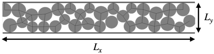
A natural question is then what will happen below the upper critical dimension. To answer this question, we here investigate the jamming transition for $d<2$. However, the jammed configuration of a true $d=1$ system is trivial: for $\varphi\geq\varphi_{J}$, the number of contacts per particle is just $z=2$, unless next nearest neighbor particles begin to interact at very high $\varphi$. To obtain non-trivial results, we consider a quasi-one-dimensional system as shown in Fig. 1, where particles are confined between the walls at $y=0$ and $y=L_{y}$. In the thermodynamic limit with fixed $L_{y}$, the model can be considered as a one-dimensional system, but the jammed configuration is still far from trivial.

In the previous works, quasi-one-dimensional systems have been studied to elucidate the effect of confinement on the jamming transition Landry et al. (2003); Desmond and Weeks (2009). These studies uncover how the confinement changes the transition point $\varphi_{J}$ Desmond and Weeks (2009) and the distribution of the stress near the walls Landry et al. (2003). However, the investigation of the critical properties is limited for the systems with very small $L_{y}$ where the jammed configuration is similar to that of the true $d=1$ system: each particle contact with at most two particles, and therefore one can not discuss the scaling of $\delta z$ Ashwin and Bowles (2009); Ashwin et al. (2013); Godfrey and Moore (2014). To our knowledge, the scaling of $\delta z$ for an intermediate value of $L_{y}$ has not been studied before.

In this work, by means of extensive numerical simulations, we show that the system is always isostatic at the jamming transition point for all values of $L_{y}$, as in the case of the jamming in $d\geq 2$. Nevertheless, the critical behavior of the jamming of the quasi-one-dimensional system is dramatically different from the jamming transition in $d\geq 2$. We find that the excess contact number $\delta z$, and the excess constraints $\delta c$, which plays a similar role as $\delta z$, exhibit the linear scaling $\delta z\sim\delta c\sim\delta\varphi$. Furthermore, we find that $g(h)$ remains finite even at $\varphi_{J}$. These results prove that the jamming transition of the quasi-one-dimensional system indeed shows the distinct scaling behaviors from those in $d\geq 2$.

Model. –

Figure 1: A configuration at $\varphi_{J}$ for $N=32$ and $L_{y}=2\sigma_{\rm max}$. Gray circles represent particles, and the solid lines denote the contacts.

Here we describe the details of our model. We consider two dimensional disks in a $L_{x}\times L_{y}$ box. For the $y$-direction, particles are confined between the walls at $y=0$ and $y=L_{y}$. For the $x$-direction, we impose the periodic boundary condition. The interaction potential of the model is given by

$$V_{N}=\sum_{i<j}^{1,N}v(h_{ij})+\sum_{i=1}^{N}v(h_{i}^{\rm b})+\sum_{i=1}^{N}v(h_{i}^{\rm t}),$$

$$h_{ij}=\left|\bm{r}_{i}-\bm{r}_{j}\right|-\frac{\sigma_{i}+\sigma_{j}}{2},$$

$$h_{i}^{\rm b}=y_{i}-\frac{\sigma_{i}}{2},\ h_{i}^{\rm t}=L_{y}-y_{i}-\frac{\sigma_{i}}{2},$$

$$v(h)=k\frac{h^{2}}{2}\theta(-h),$$ (1)

where $\bm{r}_{i}=\{x_{i},y_{i}\}$ and $\sigma_{i}$ respectively denote the position and diameter of particle $i$, $h_{ij}$ denotes the gap function between particles $i$ and $j$, and $h_{i}^{\rm b}$ and $h_{i}^{\rm t}$ respectively denote the gap functions between particle $i$ and bottom and top walls. To avoid crystallization, we consider polydisperse particles with uniform distribution $\sigma_{i}\in[\sigma_{\rm min},\sigma_{\rm max}]$. Here after we set, $k=1$, $\sigma_{\rm min}=1$, and $\sigma_{\rm max}=1.4$.

Numerics. –

We perform numerical simulations for $N=1024$ disks. We find $\varphi_{J}$ by combining slow compression and decompression as follows O’Hern et al. (2003). We first generate a random initial configuration at a small packing fraction $\varphi=0.1$ between the walls at $y=0$ and $y=L_{y}$. Then, we slowly compress the system by performing an affine transformation along the $x$-direction. For each compression step, we increase the packing fraction with a small increment $\delta\varphi=10^{-3}$, and successively minimize the energy with the FIRE algorithm Bitzek et al. (2006) until the squared force acting on each particle becomes smaller than $10^{-25}$. After arriving at a jammed configuration with $V_{N}/N>10^{-16}$, we change the sign and amplitude of the increment as $\delta\varphi\to-\delta\varphi/2$. Then, we decompress the system until we obtain an unjammed configuration with $V_{N}/N<10^{-16}$. We repeat this process by changing the sign and amplitude of the increment as $\delta\varphi\to-\delta\varphi/2$ every time the system crosses the jamming transition point. We terminate the simulation when $V_{N}/N\in(10^{-16},2\times 10^{-16})$. We define $\varphi_{J}$ as a packing fraction at the end of the above algorithm.

After obtained a configuration at $\varphi_{J}$, we re-compress the system to obtain configurations above $\varphi_{J}$. As reported in Ref. VanderWerf et al. (2020), some fraction of samples become unstable during the compression (compression unjamming). We neglect these samples. We remove the rattlers that have less than three contacts before calculating physical quantities. Hereafter, we refer the number of the non-rattler particles as $N_{\rm nr}$. To improve the statistics, we average over $50$ independent samples.

$\varphi_{J}$ and $z_{J}$. –

Figure 2: $L_{y}$ dependence of (a) the jamming transition point $\varphi_{J}$ and (b) the contact number per particle at the jamming transition point $z_{J}$. Markers denote numerical results, and solid lines denote the guide to the eye. The dashed lines denote the linear fits $\varphi_{J}=0.84-0.28\sigma_{\rm max}/L_{y}$ and $z_{J}=4-1.4\sigma_{\rm max}/L_{y}$.

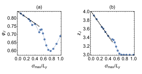
First, we discuss the $L_{y}$ dependence of the jamming transition point $\varphi_{J}$ and the contact number par particle at that point $z_{J}$. In Fig. 2 (a), we show $\varphi_{J}$ as a function of $\sigma_{\rm max}/L_{y}$. For intermediate values of $\sigma_{\rm max}/L_{y}$, $\varphi_{J}$ shows a non-monotonic behavior. A similar non-monotonic behavior has been reported in a previous numerical simulation for a binary mixture Desmond and Weeks (2009). In the limit $\sigma_{\rm max}/L_{y}\to 0$, $\varphi_{J}$ converges to its bulk value $\varphi_{J}^{\rm bulk}=0.84$ as $\varphi_{J}^{\rm bulk}-\varphi_{J}\propto 1/L_{y}$, see the dashed line in Fig. 2 (a). The same scaling has been observed in the previous simulation for the binary mixture Desmond and Weeks (2009). The scaling implies the growing length scale $\xi\sim(\varphi_{J}^{\rm bulk}-\varphi)^{-\nu}$ with $\nu=1$. It is worth mentioning that this is the same exponent observed by a correction to scaling analysis Vågberg et al. (2011) and also our replica calculation for a confined system Ikeda and Ikeda (2015).

In Fig. 2 (b), we show $z_{J}$ as a function of $\sigma_{\rm max}/L_{y}$. It is well known that $z_{J}=z_{J}^{\rm bulk}=4$ for bulk two dimensional disks O’Hern et al. (2003). In the $L_{y}\to\infty$ limit, $z_{J}$ converges to the bulk value as $z_{J}^{\rm bulk}-z_{J}\sim 1/L_{y}$, see the dashed line in Fig. 2 (b).

Isostaticity. –

Next we discuss the isostaticity of our model at $\varphi_{J}$. The number of degrees of freedom of the non-rattler particles is $N_{f}=2N_{\rm nr}-1$ where $N_{\rm nr}$ denotes the number of non-rattler particles, and we neglect the global translation along the $x$-axis. The number of constrains is

$$N_{c}=\frac{N_{\rm nr}z-N_{\rm w}}{2}+N_{\rm w}=\frac{N_{\rm nr}z}{2}+\frac{N_{\rm w}}{2},$$ (2)

where $z$ denotes the number of contacts per particle, $N_{\rm w}$ denotes the number of contacts between particles and walls, and $(N_{\rm nr}z-N_{\rm w})/2$ accounts for the number of contacts between particles.

Figure 3: $L_{y}$ dependence of the number of constraints per particle at the jamming transition point $c_{J}$. Markers denote the numerical results, and the dashed line denotes the isostatic number $c_{\rm iso}=2$.

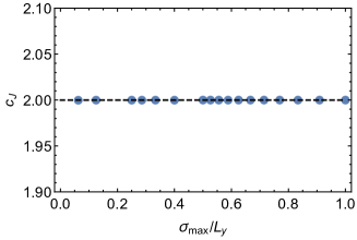
To discuss the isostaticity, we observe the number of constraints per particle $c=N_{c}/N_{\rm nr}$. When the system is isostatic $N_{c}=N_{f}$, we get $c=c_{\rm iso}=2$ in the thermodynamic limit. In Fig. 3, we show our numerical result of $c$ at $\varphi_{J}$ as a function of $\sigma_{\rm max}/L_{y}$. This plot proves that the system is always isostatic, irrespective of the value of $L_{y}$.

Now we shall discuss the behavior above $\varphi_{J}$. As mentioned in the introduction, we will investigate the model mainly for $L_{y}>2\sigma_{\rm min}$ so that some fraction of disks can pass through, and thus the contact network undergoes a non-trivial rearrangement on the change of $\varphi$.

Energy and pressure. –

For $\varphi>\varphi_{J}$, the particles overlap each other. As a consequence, the energy $V_{N}$ and pressure $p$ have finite values. Since we only consider the compression along the $x$-axis, we define the pressure as

$$p=-\frac{1}{V}\left.\frac{\partial V_{N}(\{x_{i}^{\prime}\})}{\partial\varepsilon}\right|_{\varepsilon=0}=-\frac{1}{V}\sum_{i<j}v^{\prime}(h_{ij})\frac{(x_{i}-x_{j})^{2}}{\left|\bm{r}_{i}-\bm{r}_{j}\right|},$$ (3)

where $V=L_{x}L_{y}$, and $x_{i}^{\prime}=x_{i}(1+\varepsilon)$ denotes the affine transformation along the $x$-axis.

Figure 4: (a) $\delta\varphi$ dependence of the energy per particle $V_{N}/N$. Maker denote numerical results, and the solid line denotes $\delta\varphi^{2}$. (b) $\delta\varphi$ dependence of the pressure $p$. Maker denote numerical results, and the solid line denotes $\delta\varphi$.

In Fig. 4, we show the $\delta\varphi$ dependence of $V_{N}/N$ and $p$. We find the scalings $V_{N}/N\sim\delta\varphi^{2}$ and $p\sim\delta\varphi$. The same scalings were observed for the bulk systems in $d=2$ and $d=3$ O’Hern et al. (2003).

Number of constraints and contacts. –

Next we observe the density dependence of the number of constraints. For this purpose, we introduce the excess constraints as

$$\delta c=\frac{N_{c}-(N_{f}+1)}{N_{\rm nr}}.$$ (4)

where $N_{f}+1$ denotes the minimal number of constraints to stabilize a system consisting of frictionless spherical particles Wyart (2005); Goodrich et al. (2012). For the bulk limit $L_{y}\sim\sigma_{\rm max}\sqrt{N}$, $\delta c$ can be identified with the excess contact number $\delta z$. In this case, the extensive finite size scaling analysis proved the following scaling form Goodrich et al. (2012):

$$\delta c={N}^{-1}\mathcal{C}\left({N}^{2}\delta\varphi\right),$$ (5)

where the scaling function $\mathcal{C}(x)$ behaves as

$$\mathcal{C}(x)\sim\begin{cases}x^{1/2}&x\gg 1\\ x&x\ll 1.\end{cases}$$ (6)

This implies that the square root behavior $\delta c\sim\delta\varphi^{1/2}$ is truncated at $\delta\varphi\sim N^{-2}$ for a finite $N$ system. For ${\delta\varphi\ll N^{-2}}$, one observes a linear scaling behavior ${\delta c\sim N\delta\varphi}$ Vågberg et al. (2011).

Figure 5: (a) $\delta c$ as a function of $\delta\varphi$. Markers denote numerical results. The solid and dashed lines denote $\delta c\sim\delta\varphi^{1/2}$ and $\delta c\sim\delta\varphi$, respectively. (b) Scaling plot for the same data.

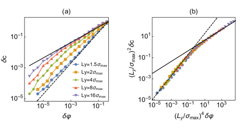
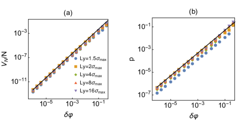
To investigate how the behavior changes for $L_{y}\ll\sigma_{\rm max}\sqrt{N}$, in Fig. 5 (a), we show the $\delta\varphi$ dependence of $\delta c$ for several $L_{y}$. For large $L_{y}$ and intermediate $\delta\varphi$, we observe the square root scaling $\delta c\sim\delta\varphi^{1/2}$. On the contrary, for small $L_{y}$ and $\delta\varphi$, $\delta c$ shows the linear behavior $\delta c\sim\delta\varphi$. To discuss the scaling behavior more closely, we assume the following scaling form:

$$\delta c=l_{y}^{\alpha}\mathcal{C}^{\prime}\left(l_{y}^{\beta}\delta\varphi\right),$$ (7)

where $l_{y}=L_{y}/\sigma_{\rm max}$, and $\mathcal{C}^{\prime}(x)$ shows the same scaling behavior as $\mathcal{C}(x)$, Eq. (6). When $l_{y}\sim\sqrt{N}$, the scaling should converge to that of the bulk $d=2$ system, Eq. (5). This requires $\alpha=-2$ and $\beta=4$. In Fig. 5, we test this prediction. A good scaling collapse verifies the scaling function Eq. (7).

Note that for a bulk system in $d\geq 2$, the system exhibits the linear scaling only for $\delta\varphi\ll N^{-2}$: the linear regime vanishes in the thermodynamic limit. Contrary, Eq. (7) implies that the linear scaling regime persists even in the thermodynamic limit for the quasi-one-dimensional system as long as $L_{y}$ is finite. Therefore, the quasi-one-dimensional system indeed has a distinct critical exponent from that of the bulk systems in $d\geq 2$.

Figure 6: (a) $z$ as a function of $\delta\varphi$. Markers denote numerical results. (b) $\delta z=z-z_{J}$ as a function of $\delta\varphi$. The solid and dashed lines denote $\delta z\sim\delta\varphi^{1/2}$ and $\delta z\sim\delta\varphi$, respectively. (c) Scaling plot for the same data.

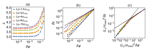
In Figs.(a)–(c), we also show the behaviors of the contact number per particle $z$, excess contacts $\delta z=z-z_{J}$, and its scaling plot. The data for $\delta z$ are more noisy than $\delta c$, presumably due to the fluctuation of $z_{J}$, but still we find a reasonable scaling collapse by using the same scaling form as $\delta c$.

Gap distribution. –

Another important quantity to characterize the critical property of the jamming transition is the gap distribution $g(h)$. For the bulk systems in $d\geq 2$, $g(h)$ exhibits the power-law divergence at $\varphi_{J}$:

$$g(h)\sim h^{-\gamma}$$ (8)

with $\gamma=0.41$ Charbonneau et al. (2014).

Figure 7: (a) CDF of the gap function $h$. Markers denote numerical results. The solid and dashed lines denote $h^{1-\gamma}$ and $h^{1}$, respectively. (b) Scaling plot for the same data.

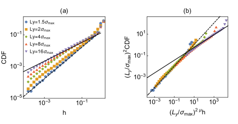
In order to improve the statistics, we observe the cumulative distribution function (CDF) of the gap functions ($h_{ij}$ and $h_{i}^{\rm t,b}$), instead of $g(h)$ itself. In this case, the power-law divergence Eq. (8) appears as ${\rm CDF}\sim h^{1-\gamma}$. In Fig. 7 (a), we show our numerical results of CDF for several $L_{y}$. We find that for small $L_{y}$ and $h$, ${\rm CDF}\sim h$ meaning that $g(h)$ remains finite $g(h)\sim h^{0}$ even at $\varphi_{J}$. On the contrary, for large $L_{y}$, there appears the intermediate regime where ${\rm CDF}\sim h^{1-\gamma}$, as in $d\geq 2$. To discuss the crossover from ${\rm CDF}\sim h$ to ${\rm CDF}\sim h^{1-\gamma}$, we assume the following scaling form:

$${\rm CDF}=l_{y}^{\zeta}\mathcal{F}^{\prime}\left(l_{y}^{\eta}h\right),$$ (9)

where the scaling function $\mathcal{F}^{\prime}(x)$ behaves as

$$\mathcal{F}^{\prime}(x)\sim\begin{cases}x^{1-\gamma}&x\gg 1\\ x&x\ll 1.\end{cases}$$ (10)

When $l_{y}\sim\sqrt{N}$, this should converge to the scaling form for finite $N$, ${\rm CDF}(h)=N^{-1}\mathcal{F}(N^{\mu}h)$, where ${\mu=1/(1-\gamma)}$, and $\mathcal{F}(x)$ shows the same scaling as Eq. (10) Ikeda et al. (2020). This requires $\zeta=-2$ and $\eta=2\mu$. In Fig. 7 (b), we check this prediction. The excellent collapse of the data for $h\ll 1$ proves the validity of our scaling Ansatz Eq. (9) .

Quasi-two-dimensional system. –

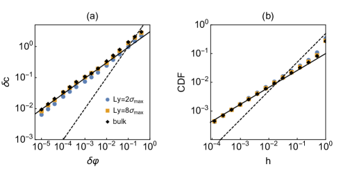
One may suspect that the distinct scaling of the quasi-one-dimensional system is due to the effect of the boundary condition, not the spatial dimensions. To investigate this possibility, we conduct a numerical simulation for a quasi-two-dimensional system. We consider the same interaction potential as Eq. (1) with the same system size $N=1024$ and polydispersity $\sigma_{i}\in[1.0,1.4]$, but this time we consider spheres in a $L_{x}\times L_{y}\times L_{z}$ box. As before, particles are confined between the walls at $y=0$ and $y=L_{y}$, and the periodic boundary conditions are imposed along the $x$ and $z$ directions. We fix $L_{y}$ and change $L_{x}=L_{z}$ to control $\varphi$. For comparison, we also perform numerical simulations for the bulk three dimensional system, where $L_{x}=L_{y}=L_{z}$ and the periodic boundary conditions are imposed for all directions. In Fig. 8, we summarize our results for $\delta c$ and CDF of the gaps. One can see that the scaling of the quasi-two-dimensional system is the same as that of the bulk three dimensional system. This result implies that the different scaling of the quasi-one-dimensional system is indeed a consequence of the fact that one dimension is lower than the upper critical dimension.

Figure 8: Results for the quasi-two-dimensional system and bulk three dimensional system. (a) $\delta c$ as a function of $\delta\varphi$. Markers denote numerical results. The solid and dashed lines denote $\delta c\sim\delta\varphi^{1/2}$ and $\delta c\sim\delta\varphi$, respectively. (b) CDF of the gap function $h$. Markers denote numerical results. The solid and dashed lines denote ${\rm CDF}\sim h^{1-\gamma}$ and ${\rm CDF}\sim h^{1}$, respectively.

Conclusions. –

In this work, we showed that the jamming transition in a quasi-one-dimensional system is qualitatively different from that in $d\geq 2$ systems: the excess constraints and contacts exhibit the linear scaling $\delta c\sim\delta z\sim\delta\varphi$, instead of the square root scaling $\delta z\sim\delta\varphi^{1/2}$, and the gap distribution $g(h)$ remains finite even at $\varphi_{J}$, instead of the power-law divergence $g(h)\sim h^{-\gamma}$.

Important future work is to test the robustness of our results for other shapes of the quasi-one-dimensional geometries such as a $d$-dimensional box with an infinite length in only one direction and fixed lengthes in the other $d-1$ directions, and circular cylinder with a fixed radius.

References

- Liu and Nagel (2010) A. J. Liu and S. R. Nagel, Annu. Rev. Condens. Matter Phys. 1, 347 (2010).
- O’Hern et al. (2003) C. S. O’Hern, L. E. Silbert, A. J. Liu, and S. R. Nagel, Phys. Rev. E 68, 011306 (2003).
- Bernal and Mason (1960) J. Bernal and J. Mason, Nature 188, 910 (1960).
- Goodrich et al. (2012) C. P. Goodrich, A. J. Liu, and S. R. Nagel, Phys. Rev. Lett. 109, 095704 (2012).
- Donev et al. (2005) A. Donev, S. Torquato, and F. H. Stillinger, Phys. Rev. E 71, 011105 (2005).
- Charbonneau et al. (2014) P. Charbonneau, J. Kurchan, G. Parisi, P. Urbani, and F. Zamponi, Nat. Commun. 5, 3725 (2014).
- Franz and Parisi (2016) S. Franz and G. Parisi, J. Phys. A 49, 145001 (2016).
- Franz et al. (2017) S. Franz, G. Parisi, M. Sevelev, P. Urbani, and F. Zamponi, SciPost Phys. 2, 019 (2017).
- Wyart et al. (2005) M. Wyart, L. E. Silbert, S. R. Nagel, and T. A. Witten, Phys. Rev. E 72, 051306 (2005).
- Yan et al. (2016) L. Yan, E. DeGiuli, and M. Wyart, EPL 114, 26003 (2016).
- DeGiuli et al. (2014) E. DeGiuli, A. Laversanne-Finot, G. Düring, E. Lerner, and M. Wyart, Soft Matter 10, 5628 (2014).
- Wyart (2005) M. Wyart, arXiv preprint cond-mat/0512155 (2005).
- Hexner et al. (2019) D. Hexner, P. Urbani, and F. Zamponi, Phys. Rev. Lett. 123, 068003 (2019).
- Landry et al. (2003) J. W. Landry, G. S. Grest, L. E. Silbert, and S. J. Plimpton, Phys. Rev. E 67, 041303 (2003).
- Desmond and Weeks (2009) K. W. Desmond and E. R. Weeks, Phys. Rev. E 80, 051305 (2009).
- Ashwin and Bowles (2009) S. S. Ashwin and R. K. Bowles, Phys. Rev. Lett. 102, 235701 (2009).
- Ashwin et al. (2013) S. S. Ashwin, M. Zaeifi Yamchi, and R. K. Bowles, Phys. Rev. Lett. 110, 145701 (2013).
- Godfrey and Moore (2014) M. J. Godfrey and M. A. Moore, Phys. Rev. E 89, 032111 (2014).
- Bitzek et al. (2006) E. Bitzek, P. Koskinen, F. Gähler, M. Moseler, and P. Gumbsch, Phys. Rev. Lett. 97, 170201 (2006).
- VanderWerf et al. (2020) K. VanderWerf, A. Boromand, M. D. Shattuck, and C. S. O’Hern, Phys. Rev. Lett. 124, 038004 (2020).
- Vågberg et al. (2011) D. Vågberg, D. Valdez-Balderas, M. A. Moore, P. Olsson, and S. Teitel, Phys. Rev. E 83, 030303(R) (2011).
- Ikeda and Ikeda (2015) H. Ikeda and A. Ikeda, EPL 111, 40007 (2015).
- Ikeda et al. (2020) H. Ikeda, C. Brito, and M. Wyart, J. Stat. Mech.: Theory Exp. 2020, 033302 (2020).
- Note (1) Note that our scaling prediction does not work for , where CDF does not show the power-law behavior Charbonneau et al. (2012).
- Charbonneau et al. (2012) P. Charbonneau, E. I. Corwin, G. Parisi, and F. Zamponi, Phys. Rev. Lett. 109, 205501 (2012).