Balancing reconstruction error and Kullback-Leibler divergence in Variational Autoencoders

Abstract

In the loss function of Variational Autoencoders there is a well known tension between two components: the reconstruction loss, improving the quality of the resulting images, and the Kullback-Leibler divergence, acting as a regularizer of the latent space. Correctly balancing these two components is a delicate issue, easily resulting in poor generative behaviours. In a recent work TwoStage , a sensible improvement has been obtained by allowing the network to learn the balancing factor during training, according to a suitable loss function. In this article, we show that learning can be replaced by a simple deterministic computation, helping to understand the underlying mechanism, and resulting in a faster and more accurate behaviour. On typical datasets such as Cifar and Celeba, our technique sensibly outperforms all previous VAE architectures.

1 Introduction

Generative models address the challenging task of capturing the probabilistic distribution of high-dimensional data, in order to gain insight in their characteristic manifold, and ultimately paving the way to the possibility of synthesizing new data samples.

The main frameworks of generative models that have been investigated so far are Generative Adversarial Networks (GAN) GAN and Variational Autoencoders (VAE) (Kingma13 ; RezendeMW14 ), both of which generated an enormous amount of works, addressing variants, theoretical investigations, or practical applications.

The main feature of Variational Autoencoders is that they offer a strongly principled probabilistic approach to generative modeling. The key insight is the idea of addressing the problem of learning representations as a variational inference problem, coupling the generative model $P(X|z)$ for $X$ given the latent variable $z$, with an inference model $Q(z|X)$ synthesizing the latent representation of the given data.

The loss function of VAEs is composed of two parts: one is just the log-likelihood of the reconstruction, while the second one is a term aimed to enforce a known prior distribution $P(z)$ of the latent space - typically a spherical normal distribution. Technically, this is achieved by minimizing the Kullbach-Leibler distance between $Q(z|X)$ and the prior distribution $P(z)$; as a side effect, this will also improve the similarity of the aggregate inference distribution $Q(z)=\operatorname{\mathbb{E}}_{X}Q(z|Z)$ with the desired prior, that is our final objective.

$$\hskip 14.22636pt\underbrace{\operatorname{\mathbb{E}}_{z\sim Q(z|X)}log(P(X|z))}_{log-likelihood}-\lambda\cdot\underbrace{KL(Q(z|X)||P(z))}_{KL-divergence}$$

Loglikelihood and KL-divergence are typically balanced by a suitable $\lambda$-parameter (called $\beta$ in the terminology of $\beta$-VAE beta-vae17 ; understanding-beta-vae18 ), since they have somewhat contrasting effects: the former will try to improve the quality of the reconstruction, neglecting the shape of the latent space; on the other side, KL-divergence is normalizing and smoothing the latent space, possibly at the cost of some additional “overlapping” between latent variables, eventually resulting in a more noisy encoding brokenELBOW . If not properly tuned, KL-divergence can also easily induce a sub-optimal use of network capacity, where only a limited number of latent variables are exploited for generation: this is the so called overpruning/variable-collapse/sparsity phenomenon BurdaGS15 ; overpruning17 .

Tuning down $\lambda$ typically reduces the number of collapsed variables and improves the quality of reconstructed images. However, this may not result in a better quality of generated samples, since we loose control on the shape of the latent space, that becomes harder to be exploited by a random generator.

Several techniques have been considered for the correct calibration of $\gamma$, comprising an annealed optimization schedule Bowman15 or a policy enforcing minimum KL contribution from subsets of latent units autoregressive16 . Most of these schemes require hand-tuning and, quoting overpruning17 , they easily risk to “take away the principled regularization scheme that is built into VAE.”

An interesting alternative that has been recently introduced in TwoStage consists in learning the correct value for the balancing parameter during training, that also allows its automatic calibration along the training process. The parameter is called $\gamma$, in this context, and it is considered as a normalizing factor for the reconstruction loss.

Measuring the trend of the loss function and of the learned lambda parameter during training, it becomes evident that the parameter is proportional to the reconstruction error, with the result that the relevance of the KL-component inside the whole loss function becomes independent from the current error.

Considering the shape of the loss function, it is easy to give a theoretical justification for this behavior. As a consequence, there is no need for learning, that can be replaced by a simple deterministic computation, eventually resulting in a faster and more accurate behaviour.

The structure of the article is the following. In Section 2, we give a quick introduction to Variational Autoencoders, with particular emphasis on generative issues (Section 2.1). In Section 3, we discuss our approach to the problem of balancing reconstruction error and Kullback-Leibler divergence in the VAE loss function; this is obtained from a simple theoretical investigation of the loss function in TwoStage , and essentially amounts to keeping a constant balance between the two components along training. Experimental results are provided in Section 4, relative to standard datasets such as CIFAR-10 (Section 4.1) and CelebA (Section 4.2): up to our knowledge, we get the best generative scores in terms of Frechet Inception Distance ever obtained by means of Variational Autoencoders. In Section 5, we try to investigate the reasons why our technique seems to be more effective than previous approaches, by considering the evolution of latent variables along training. Concluding remarks and ideas for future investigations are offered in Section 5.1.

2 Variational Autoencoders

In a generative setting, we are interested to express the probability of a data point $X$ through marginalization over a vector of latent variables:

$$\hskip 14.22636ptP(X)=\int P(X|z)P(z)dz\approx\operatorname{\mathbb{E}}_{z\sim P(z)}P(X|z)$$ (1)

For most values of $z$, $P(X|z)$ is likely to be close to zero, contributing in a negligible way in the estimation of $P(X)$, and hence making this kind of sampling in the latent space practically unfeasible. The variational approach exploits sampling from an auxiliary “inference” distribution $Q(z|X)$, hopefully producing values for $z$ more likely to effectively contribute to the (re)generation of $X$. The relation between $P(X)$ and $\operatorname{\mathbb{E}}_{z\sim Q(z|X)}P(X|z)$ is given by the following equation, where KL denotes the Kulback-Leibler divergence:

$$\hskip 8.5359pt\begin{array}[]{l}log(P(X))-KL(Q(z|X)||P(z|X))=\\ \hskip 14.22636pt\operatorname{\mathbb{E}}_{z\sim Q(z|X)}log(P(X|z)-KL(Q(z|X)||P(z))\end{array}$$ (2)

KL-divergence is always positive, so the term on the right provides a lower bound to the loglikelihood $P(X)$, known as Evidence Lower Bound (ELBO).

If $Q(z|X)$ is a reasonable approximation of $P(z|X)$, the quantity $KL(Q(z)||P(z|X))$ is small; in this case the loglikelihood $P(X)$ is close to the Evidence Lower Bound: the learning objective of VAEs is the maximization of the ELBO.

In traditional implementations, we additionally assume that $Q(z|X)$ is normally distributed around an encoding function $\mu_{\theta}(X)$, with variance $\sigma^{2}_{\theta}(X)$; similarly $P(X|z)$ is normally distributed around a decoder function $d_{\theta}(z)$. The functions $\mu_{\theta}$, $\sigma^{2}_{\theta}$ and $d_{\theta}$ are approximated by deep neural networks. Knowing the variance of latent variables allows sampling during training.

Provided the model for the decoder function $d_{\theta}(z)$ is sufficiently expressive, the shape of the prior distribution $P(z)$ for latent variables can be arbitrary, and for simplicity we may assumed it is a normal distribution $P(z)=G(0,1)$. The term $KL(Q(z|X)||P(z)$ is hence the KL-divergence between two Gaussian distributions $G(\mu_{\theta}(X),\sigma^{2}_{\theta}(X))$ and $G(1,0)$ which can be computed in closed form:

$$\hskip 8.5359pt\begin{array}[]{l}KL(G(\mu_{\theta}(X),\sigma_{\theta}(X)),G(0,1))=\\ \hskip 28.45274pt\frac{1}{2}(\mu_{\theta}(X)^{2}+\sigma^{2}_{\theta}(X)-log(\sigma^{2}_{\theta}(X))-1)\end{array}$$ (3)

As for the term $\operatorname{\mathbb{E}}_{z\sim Q(z|X)}log(P(X|z)$, under the Gaussian assumption the logarithm of $P(X|z)$ is just the quadratic distance between $X$ and its reconstruction $d_{\theta}(z)$; the $\lambda$ parameter balancing reconstruction error and KL-divergence can understood in terms of the variance of this Gaussian (tutorial-VAE ).

The problem of integrating sampling with backpropagation, is solved by the well known reparametrization trick (VAE13 ; RezendeMW14 ).

2.1 Generation of new samples

The whole point of VAEs is to force the generator to produce a marginal distribution $Q(z)=\operatorname{\mathbb{E}}_{X}Q(z|X)$ close to the prior $P(z)$. If we average the Kullback-Leibler regularizer $KL(Q(z|X)||P(z))$ on all input data, and expand KL-divergence in terms of entropy, we get:

$$\hskip 14.22636pt\begin{array}[]{l}\operatorname{\mathbb{E}}_{X}KL(Q(z|X)||P(z))\vskip 3.0pt plus 1.0pt minus 1.0pt\\ \vskip 3.0pt plus 1.0pt minus 1.0pt=-\operatorname{\mathbb{E}}_{X}\mathcal{H}(Q(z|X))+\operatorname{\mathbb{E}}_{X}\mathcal{H}(Q(z|X),P(z))\\ \vskip 3.0pt plus 1.0pt minus 1.0pt=-\operatorname{\mathbb{E}}_{X}\mathcal{H}(Q(z|X))+\operatorname{\mathbb{E}}_{X}\operatorname{\mathbb{E}}_{z\sim Q(z|X)}logP(z)\\ \vskip 3.0pt plus 1.0pt minus 1.0pt=-\operatorname{\mathbb{E}}_{X}\mathcal{H}(Q(z|X))+\operatorname{\mathbb{E}}_{z\sim Q(z)}logP(z)\\ \vskip 3.0pt plus 1.0pt minus 1.0pt=-\underbrace{\operatorname{\mathbb{E}}_{X}\mathcal{H}(Q(z|X))}_{\begin{subarray}{c}\mbox{Avg. Entropy}\\ \mbox{of }Q(z|X)\end{subarray}}+\underbrace{\mathcal{H}(Q(z),P(z))}_{\begin{subarray}{c}\mbox{Cross-entropy }\\ \mbox{of }Q(X)\mbox{ vs }P(z)\end{subarray}}\end{array}$$ (4)

The cross-entropy between two distributions is minimal when they coincide, so we are pushing $Q(z)$ towards $P(z)$. At the same time, we try to augment the entropy of each $Q(z|X)$; under the assumption that $Q(z|X)$ is Gaussian, this amounts to enlarge the variance, further improving the coverage of the latent space, essential for generative sampling (at the cost of more overlapping, and hence more confusion between the encoding of different datapoints).

Since our prior distribution is a Gaussian, we expect $Q(z)$ to be normally distributed too, so the mean $\mu$ should be 0 and the variance $\sigma^{2}$ should be 1. If $Q(z|X)=N(\mu(X),\sigma^{2}(X))$, we may look at $Q(z)=\operatorname{\mathbb{E}}_{X}Q(z|X)$ as a Gaussian Mixture Model (GMM). Then, we expect

$$\hskip 85.35826pt\operatorname{\mathbb{E}}_{X}\mu(X)=0$$ (5)

and especially, assuming the previous equation (see aboutVAE for details),

$$\hskip 56.9055pt\sigma^{2}=\operatorname{\mathbb{E}}_{X}\mu(X)^{2}+\operatorname{\mathbb{E}}_{X}\sigma^{2}(X)=1$$ (6)

This rule, that we call variance law, provides a simple sanity check to test if the regularization effect of the KL-divergence is properly working.

The fact that the two first moments of the marginal inference distribution are 0 and 1, does not imply that it should look like a Normal. The possible mismatching between $Q(z)$ and the expected prior $P(z)$ is indeed a problematic aspect of VAEs that, as observed in several works ELBOsurgery ; rosca2018distribution ; aboutVAE could compromise the whole generative framework. To fix this, some works extend the VAE objective by encouraging the aggregated posterior to match $P(z)$ WAE or by exploiting more complex priors autoregressive ; Vamp ; resampledPriors .

In TwoStage (that is the current state of the art), a second VAE is trained to learn an accurate approximation of $Q(z)$; samples from a Normal distribution are first used to generate samples of $Q(z)$, that are then fed to the actual generator of data points. Similarly, in deterministic , the authors try to give an ex-post estimation of $Q(z)$, e.g. imposing a distribution with a sufficient complexity (they consider a combination of 10 Gaussians, reflecting the ten categories of MNIST and Cifar10).

3 The balancing problem

As we already observed, the problem of correctly balancing reconstruction error and KL-divergence in the loss function has been the object of several investigations. Most of the approaches were based on empirical evaluation, and often required manual hand-tuning of the relevant parameters. A more theoretical approach has been recently pursued in TwoStage

The generative loss (GL), to be summed with the KL-divergence, is defined by the following expression (directly borrowed from the public code):

$$\hskip 56.9055ptGL=\frac{\mbox{mse}}{2\gamma^{2}}+log\gamma+\frac{log2\pi}{2}$$ (7)

where mse is the mean square error on the minibatch under consideration and $\gamma$ is a parameter of the model, learned during training. The previous loss is derived in TwoStage by a complex analysis of the VAE objective function behavior, assuming the decoder has a gaussian error with variance $\gamma^{2}$, and investigating the case of arbitrarily small but explicitly nonzero values of $\gamma^{2}$.

Since $\gamma$ has no additional constraints, we can explicitly minimize it in equation 7. The derivative $GL^{\prime}$ of $GL$ is

$$\hskip 71.13188ptGL^{\prime}=-\frac{\mbox{mse}}{\gamma^{3}}+\frac{1}{\gamma}$$ (8)

having a zero for $\gamma^{2}=\mbox{mse}$, corresponding to a minimum for equation 7.

This suggests a very simple deterministic policy for computing $\gamma$ instead of learning it: just use the current estimation of the mean square error. This can be easily computed as a discounted combination of the mse relative to the current minibatch with the previous approximation: in our implementation, we just take the minimum between these two values, in order to have a monotically decreasing value for $\gamma$ (we work with minibatches of size 100, that is sufficiently large to provide a reasonable approximation of the real mse). Updating is done at every minibatch of samples.

Compared with the original approach in TwoStage , the resulting technique is both faster and more accurate.

An additional contribution of our approach is to bring some light on the effect of the balancing technique in TwoStage . Neglecting constant addends, that have no role in the loss function, the total loss function for the VAE is simply:

$$\hskip 85.35826ptGL=\frac{\mbox{mse}}{2\gamma^{2}}+KL$$ (9)

So, computing gamma according to the previous estimation of mse has essentially the effect of keeping a constant balance between reconstruction error and KL-divergence during the whole training: as mse is decreasing, we normalize it in order to prevent a prevalence of the KL-component, that would forbid further improvements of the quality of reconstructions.

4 Empirical evaluation

We compared our proposed Two Stage VAE with computed $\gamma$ against the original model with learned $\gamma$ using the same network architectures. In particular, we worked with many different variants of the so called ResNet version, schematically described in Figure 1 (pictures are borrowed from TwoStage ).

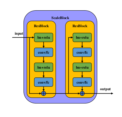
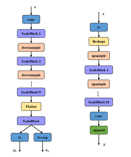
(A) Scale block	(B) Encoder   (C) decoder

Figure 1: ”Resnet” architecture. (A) Scale block: a sequence of residual blocks. We mostly worked with a single residual block; two or more blocks makes the architecture sensibly heavier and slower to train, with no remarkable improvement (B) Encoder: the input is first transformed by a convolutional layer into and then passed to a chain of Scale blocks; after each Scale block, input is downsampled with a a convolutional layer with stride $2$ channels are doubled. After $N$ Scale blocks, the feature map is flattened to a vector. and then fed to another Scale Block composed by fully connected layers of dimension 512. The output of this Scale Block is used to produce mean and variances of the $k$ latent variables. Following TwoStage , $N=3$ and $k=64$ for CIFAR-10. For CelebA, we tested many different configurations. (C) Decoder: the latent representation $z$ is first passed through a fully connected layer, reshaped to 2D, and then passed through a sequence of deconvolutions halving the number of channels at the same.

In all our experiments, we used a batch size of 100, and adopted Adam with default TensorFlow’s hyperparameters as optimizer. Other hyperparameters, as well as additional architectural details will be described below, where we discuss the cases of Cifar and CelebA separately.

In general, in all our experiments, we observed a high sensibility of Fid scores to the learning rate, and to the deployment of auxiliary regularization techniques. As we shall discuss in Section 5, modifying these training configurations may easily result in a different number of inactive latent variables at the end of training. Having both too few or too many active variables may eventually compromise generative sampling, for opposite reasons: few active variables usually compromise reconstruction quality, but an excessive number of active variables makes controlling the shape of the latent space sensbibly harder.

The code is available on GitHub. Checkpoints for Cifar10 and CelebA are available at the project’s page.

4.1 Cifar10

For Cifar10, we got relatively good results with the basic ResNet architecture with 3 Scale Blocks, a single Resblock for every Scaleblock, and 64 latent variables. We trained our model for 700 epochs on the first VAE and 1400 epochs on the second VAE; the initial learning rate was $0.0001$, halving it every $200$ epochs on the first VAE and every $100$ epochs on the second VAE. Details about the evolution of reconstruction and generative error during training are provided in Figure 2 and Table 1. The data refer to ten different but “uniform” trainings ending with the same number of active latent variables, (17 in this case). Few pathological trainings resulting in less or higher sparsity (and worse FID scores) have been removed from the statistic.

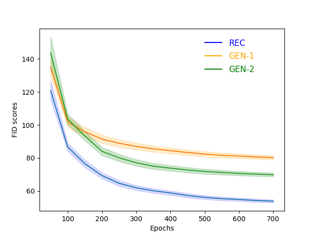
Figure 2: Evolution during 700 epochs of training on the CIFAR-10 dataset of the FID scores for reconstructed images (blue), first-stage generated images (orange), and second-stage generated images. The number of epochs refer to the first VAE, and it is doubled for the second VAE. The filled region around the line corresponds to the standard deviation from the expected value. Mean and variances have been estimated over 10 different trainings.

Table 1: Evolution during training on the CIFAR-10 dataset of several different metrics

$\begin{array}[]{|r|c|c|c|c|c|}\hline\cr\mbox{epochs}&\mbox{REC}&\mbox{GEN-1}&\mbox{GEN-2}&\mbox{mse}&\mbox{variance law}\\ \hline\cr 50&120.9\pm 5.8&134.9\pm 5.9&143.8\pm 9.7&.0089\pm.0002&1.012\pm.012\\ \hline\cr 100&86.6\pm 2.5&101.8\pm 3.1&103.5\pm 3.2&.0071\pm.0001&.969\pm.010\\ \hline\cr 150&76.5\pm 2.3&95.9\pm 2.8&93.3\pm 2.8&.0062\pm.0001&.939\pm.011\\ \hline\cr 200&69.3\pm 2.1&91.4\pm 2.5&84.0\pm 2.5&.0056\pm.0001&.918\pm.012\\ \hline\cr 250&64.6\pm 2.0&88.9\pm 2.3&80.1\pm 2.2&.0052\pm.0001&.922\pm.013\\ \hline\cr 300&61.9\pm 1.8&87.0\pm 2.1&77.1\pm 2.0&.0049\pm.0001&.925\pm.012\\ \hline\cr 350&60.1\pm 1.7&85.5\pm 1.9&75.0\pm 1.8&.0047\pm.0001&.928\pm.010\\ \hline\cr 400&58.8\pm 1.5&84.4\pm 1.8&73.8\pm 1.7&.0046\pm.0001&.930\pm.008\\ \hline\cr 450&57.2\pm 1.3&83.3\pm 1.7&72.7\pm 1.6&.0045\pm.0001&.937\pm.007\\ \hline\cr 500&56.1\pm 1.2&82.3\pm 1.6&71.8\pm 1.5&.0044\pm.0001&.942\pm.007\\ \hline\cr 550&55.3\pm 1.1&81.7\pm 1.5&71.2\pm 1.4&.0043\pm.0001&.946\pm.007\\ \hline\cr 600&54.8\pm 1.1&81.2\pm 1.4&70.6\pm 1.3&.0043\pm.0001&.950\pm.006\\ \hline\cr 650&54.2\pm 1.0&80.7\pm 1.4&70.2\pm 1.2&.0042\pm.0001&.954\pm.005\\ \hline\cr 700&53.8\pm 0.9&80.2\pm 1.3&69.8\pm 1.1&.0041\pm.0001&.957\pm.005\\ \hline\cr\end{array}$

Table 2: CIFAR-10: summary of results

model	epochs	REC	GEN-1	GEN-2
RAE-l2 deterministic (128 vars)	100	$32.24\pm?$	$80.8\pm?$	$74.2\pm?$
2S-VAE, learned $\gamma$ TwoStage	1000		$76.7\pm 0.8$	$72.9\pm 0.9$
2S-VAE, learned $\gamma$, replicated	1000	$54.1\pm 0.9$	$76.8\pm 1.2$	$73.1\pm 1.2$
2S-VAE, computed $\gamma$	700	$53.8\pm 0.9$	$80.2\pm 1.3$	${\bf 69.8}\pm 1.1$

In Table 2), we compare our approach with the original version with learned $\gamma$TwoStage . Since some people had problems in replicating the results in TwoStage (see the discussion on OpenReview), we repeated the experiment (also in order to compute the reconstruction FID). Using the learning configuration suggested by the authors, namely 1000 epochs for the first VAE, 2000 epochs for the second one, initial learning rate equal to 0.0001, halved every 300 and 600 epochs for the two stages, respectively, we obtained results essentially in line with those declared in TwoStage .

Table 3: CelebA: metrics for different models

learned $$\gamma$$ computed

Model epochs REC GEN-1 GEN-2 mse var.law REC GEN-1 GEN-2 mse var.law

1 40/120 53.8 66.0 59.3 .0059 1.024 45.8 56.9 57.1 .0056 0.805

1 80/210 54.3 65.9 59.8 .0049 0.803 46.0 61.1 58.1 .0047 0.688

1 120/300 54.9 66.5 60.4 .0044 0.775 48.1 63.8 59.9 .0043 0.687

2 40/120 48.5 58.2 54.5 .0059 0.985 41.5 58.7 53.7 .0058 1.024

2 80/210 48.8 60.7 55.5 .0048 0.889 42.0 58.8 55.1 .0048 0.877

2 120/300 49.1 62.8 56.9 .0043 0.880 43.0 60.2 56.2 .0043 0.863

3 40/120 59.4 74.3 63.4 .0050 0.893 56.3 74.0 63.9 .0049 0.637

3 80/210 55.6 72.6 62.2 .0039 0.840 54.4 72.3 61.8 .0038 0.621

3 120/300 55.2 72.0 62.1 .0037 0.785 54.4 71.3 62.0 .0036 0.744

4 40/120 52.8 68.2 60.4 .0072 0.789 48.0 65.0 57.7 .0072 0.742

4 80/210 49.4 67.9 58.5 .0060 0.822 45.3 65.0 53.4 .0059 0.785

4 120/300 49.1 68.0 58.4 .0053 0.844 44.4 65.4 54.0 .0053 0.804

For the sake of completeness, we also compare with the FID scores for the recent RAE-l2 model deterministic (variance was not provided by authors). In this case, the comparison is purely indicative, since in deterministic they work, in the CIFAR-10 case, with a latent space of dimension 128. This also explains their particularly good reconstruction error, and the few training epochs.

4.2 CelebA

In the case of CelebA, we had more trouble in replicating the results of TwoStage , although we were working with their own code. As we shall see, this was partly due to a mistake on our side, that pushed us to an extensive investigation of different architectures.

In Table 3 we summarize some of the results we obtained, over a large variety of different network configurations. The metrics given in the table refer to the following models:

• Model 1: This is our base model, with 4 scale blocks in the first stage, 64 latent variables, and dense layers with inner dimension 4096 in the second stage.

• Model 2: As Model 1 with l2 regularizer added in upsampling and scale layers in the decoder.

• Model 3: Two resblocks for every scale block, l2 regularizer added in downsampling layers in the encoder.

• Model 4: As Model 1 with 128 latent variables, and 3 scale blocks.

All models have been trained with Adam, with an initial learning rate of 0.0001, halved every 48 epochs in the first stage and every 120 epochs in the second stage.

According to the results in Table 3, we can do a few noteworthy observations:

1. for a given model, the technique computing $\gamma$ systematically outperforms the version learning it, both in reconstruction and generation on both stages;

2. after the first 40 epochs, FID scores (comprising reconstruction FID) do not seem to improve any further, and can even get worse, in spite of the fact that the mean square error keep decreasing; this is in contrast with the intuitive idea that FID REC score should be proportional to mse;

3. the variance law is far from one, that seems to suggest Kl is too weak, in this case; this justifies the mediocre generative scores of the first stage, and the sensible improvement obtained with the second stage;

4. l2-regularization, as advocated in deterministic , seems indeed to have some beneficial effect.

We spent quite a lot of time trying to figure out the reasons of the discrepancy between our observations, and the results claimed in TwoStage . Inspecting the elements of the dataset with worse reconstruction errors, we remarked a particularly bad quality of some of the images, resulting from the resizing of the face crop of dimension 128x128 to the canonical dimension 64x64 expected from the neural network. The resizing function used in the source code of TwoStage available at was the deprecated imresize function of the scipy library. Following the suggestion in the documentation, we replaced the call to imresize with a call to PILLOW:
numpy.array(Image.fromarray(arr).resize())
Unfortunately, and surprisingly, the default resizing mode of PILLOW is Nearest Neighbours that, as described in Figure 3, introduces annoying jaggies that sensibly deteriorate the quality of images.

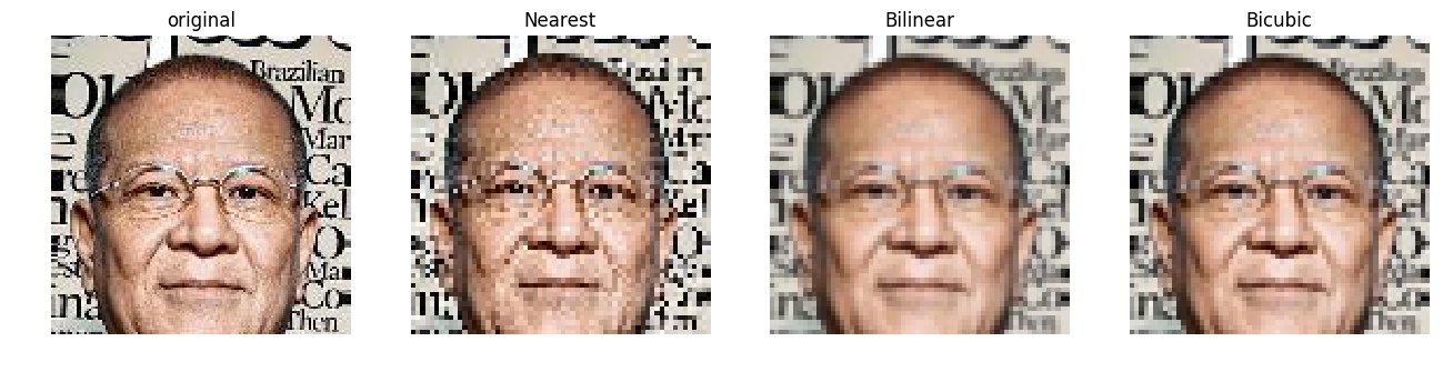
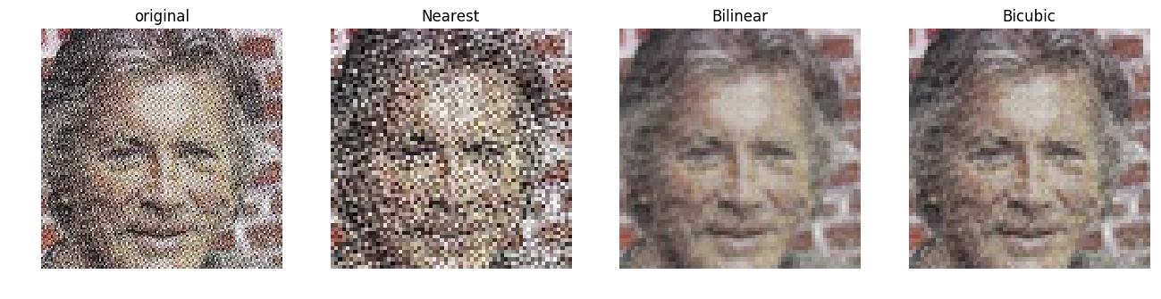
Figure 3: Effect of resizing mode on a few CelebA samples. Nearest Neighbours produces bad staircase effects; bilinear, that is the common choice, is particularly smooth, suiting well to VAEs; bicubic is sligtly sharper.

This probably also explains the anomalous behaviour of FID REC with respect to mean squared error. The Variational Autoencoder fails to reconstruct images with high frequency jaggies, while keep improving on smoother images. This can be experimentally confirmed by the fact that while the minimum mse keeps decreasing during training, the maximum, after a while, stabilizes. So, in spite of the fact that the average mse decreases, the overall distribution of reconstructed images may remain far from the distribution of real images, and possibly get even more more distant.

Table 4: CelebA: summary of results

model	epochs	REC	GEN-1	GEN-2
RAE-SN deterministic	70	$36.0\pm?$	$44.7\pm?$	$40.9\pm?$
2S-VAE, learned $\gamma$ TwoStage	120		$60.5\pm 0.6$	$44.4\pm 0.7$
2S-VAE, computed $\gamma$	70	${\bf 33.9}\pm 0.8$	${\bf 43.6}\pm 1.3$	$42.7\pm 1.0$
with latent space norm.				${\bf 38.6}\pm 1.0$

Resizing images with the traditional bilinear interpolation produces a substantial improvement, but not sufficient to obtain the expected generative scores.

Another essential component is again the balance between reconstruction error and KL-divergence. As observed above, in the case of CelebA the KL-divergence seems too weak, as clearly testified by the moments of latent variables expressed by the variance law. As a matter of fact, in the loss function of TwoStage , both mse and KL-divergence are computed as reduced sums, respectively over pixels and latent variables. Now, passing from CIFAR-10 to Celeba, we multiplied the number of pixels by four, passing from 32x32 to 64x64, but kept a constant number of latent variables. So, in order to keep the same balance we used for CIFAR-10, we should multiply the KL-divergence by a factor 4.

Finally, learning seems to proceed quite fast in the case of CelebA, that suggests to work with a lower initial learning rate: 0.00005. We also kept l2 regularization on downsampling and upsampling layers.

With these simple expedients, we were already able to improve on generative scores in TwoStage , (see Table 4), but not with respect to deterministic .

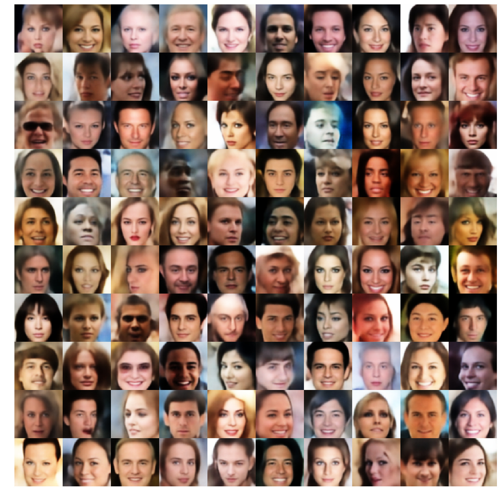
Figure 4: Examples of generated faces. The resulting images do not show the blurred appearance so typical of variational approaches, sensibly improving their perceptive quality.

Analyzing the moments of the distribution of latent variables generated during the second stage, we observed that the actual variance was sensibly below the expected unitary variance (around .85). The simplest solution consists in normalizing the generated latent variables, to meet the expected variance (this point is a bit outside the scope of this contribution, and will be better investigated in a forthcoming article).

This final precaution caused a sudden burst in the FID score for generated images, permitting to obtain, to the best of our knowledge, the best generative scores ever produced for CelebA with a variational approach.

In Figure 4 we provide examples of randomly generated faces. Note the particularly sharp quality of the images, so unusual for variational approaches.

5 Discussion

The reason why the balancing policy between reconstruction error and KL-regularization addressed in TwoStage and revisited in this article is so effective seems to rely on its laziness in the choice of the latent representation.

A Variational Autoencoder computes, for each latent variable $z$ and each sample $X$, an expected value $\mu_{z}(X)$ and a variance $\sigma^{2}_{z}(X)$ around it. During training, the variance $\sigma^{2}_{z}(X)$ usually drops very fast to values close to $0$, reflecting the fact that the network is highly confident in its choice of $\mu_{z}(X)$. The KL-component in the loss function can be understood as a mechanism aimed to reduce this confidence, by forcing a not negligible variance. By effect of the KL-regularization, some latent variables may be even neglected by the VAE, inducing sparsity in the resulting encoding sparsity . The “collapsed” variables have, for any $X$, a value of $\mu_{z}(X)$ close to $0$ and a mean variance $\sigma^{2}_{z}(X)$ close $1$. So, typically, at a relatively early stage of training, the mean variance $\operatorname{\mathbb{E}}_{X}\sigma^{2}_{z}(X)$ of each latent variable $z$ gets either close to $0$, if the variable is exploited, of close to $1$ if the variable is neglected (see Figure 5).

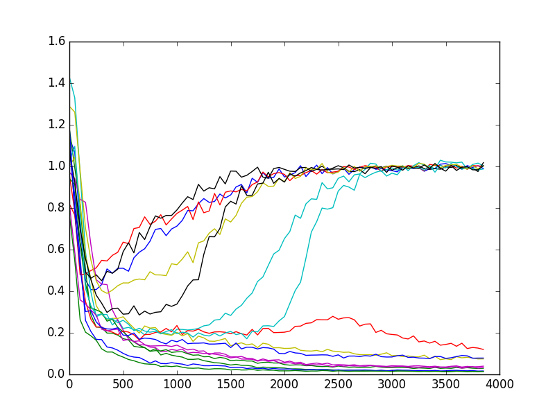
Figure 5: Typical evolution of the mean variance $\operatorname{\mathbb{E}}_{X}\sigma^{2}_{z}(X)$ of latent variables during training in a Variational Autoencoder. Relevant variables have a variance close to $0$, while inactive variables have a variance going to $1$. The picture was borrowed from sparsity and is relative to the first epoch of training for a dense VAE over the MNIST data set.

Traditional balancing policies addressed in the literature start with a low value for the KL-regularization, increasing it during training. The general idea is to start privileging the quality of reconstruction, and then try to induce a better coverage of the latent space. Unfortunately, this reshaping ex post of the latent space looks hard to achieve, in practice.

The balancing property discussed in this article does the opposite: it starts attributing a relatively high importance to KL-divergence, to balance the high initial reconstruction error, progressively reducing its relevance in a way proportional to the improvement of the reconstruction. In this way, the relative importance between the two components of the loss function remains constant during training.

The practical effect is that latent variables are kept for a long time in a sort of limbo from which, one at a time, they are retrieved and put to work by the autoencoder, as soon as it realizes how they can contribute to the reconstruction.

The previous behaviour is evident by looking at the evolution of the mean variance $\operatorname{\mathbb{E}}_{X}\sigma^{2}_{z}(X)$ of latent variables during training (not to be confused with the variance of the mean values $\mu_{z}(X)$, that according to the variance law should approximately be the complement to $1$ of the former).

In Figure 6

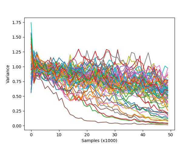
Figure 6: Evolution of the mean variance of the 64 latent variables during the first epoch of training on Cifar10. Due to the ”lazy” balancing technique, even after a full epoch, the destiny of most latent variables is still uncertain: they could collapse or be exploited for reconstruction.

we see the evolution of the variance of the 64 latent variables during the first epoch of training on the Cifar10 data set: even after a full epoch, the “status” of most latent variables is still uncertain.

During the next 50 epochs, in a very slow process, some of the “dormient” latent variables are woken up by the autoencoder, causing their mean variance to move towards 0: see Figure 7.

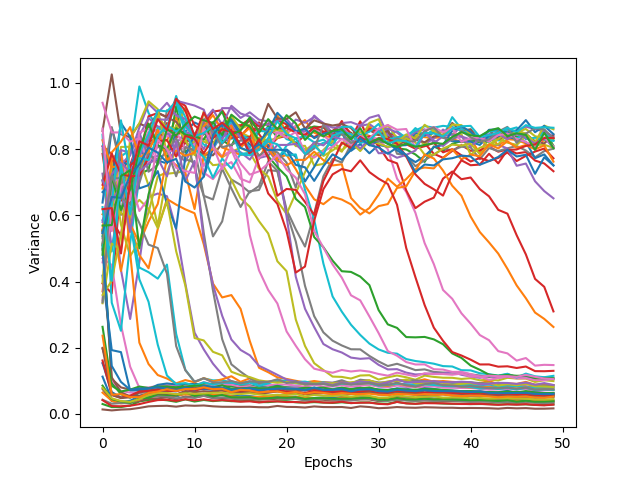
Figure 7: Evolution of the mean variance of the 64 latent variables First 50 epochs of training on Cifar10. One by one, latent variables are retrieved from the limbo (variance around 0.8) , and put to work by the autoencoder.

With the progress of training, less and less variables change their status, until the process finally stabilizes.

It would be nice to think, as hinted to in TwoStage , that the number of active latent variables at the end of training corresponds to the actual dimensionality of the data manifold. Unfortunately, this number still depends on too many external factors to justify such a claim. For instance, a mere modification of the learning rate is sensibly affecting the sparsity of the resulting latent space, as shown in Table 5 where we compare, for different initial learning rates (l.r.), the final number of inactive variables, FID scores, and mean square error.

Table 5: Effect of the learning rate on sparsity and different metrics. A high learning rate reduces sparsity and improves on reconstruction. However, this does not result in a better generative score. With a low rate, too many variables remains inactive.

l.r.	inact.	REC	GEN-1	GEN-2	mse
.00020	13	53.0	80.6	74.5	.0039
.00015	15	53.3	79.9	71.8	.0040
.00010	17	53.8	80.2	68.8	.0041
.00005	19	58.2	83.2	75.8	.0047

Specifically, a high learning rate appears to be in conflict with the lazy way we would like latent variables to be chosen for activation; this typically results in less sparsity, that is not always beneficial for generative purposes. The annoying point is that with respect to the dimensionality of the latent space with the best generative FID, activating more variables can result in a lower reconstruction error, that should not be the case if we correctly identified the datafold dimensionality.

So, while the balancing strategy discussed in this article (similarly to the one in TwoStage ) is eventually beneficial, still could take advantage of some tuning.

5.1 Conclusions

In this article, we stressed the importance of keeping a constant balance between reconstruction error and Kullback-Leibler divergence during training of Variational Autoencoders. We did so by normalizing the reconstruction error by an estimation of its current value, derived from minibatches. We developed the technique by an investigation of the loss function used in TwoStage , where the balancing parameter was instead learned during training. Our technique seems to outperform all previous Variational Approaches, permitting us to obtain unprecedented FID scores for traditional datasets such as CIFAR-10 and CelebA.

In spite of its relevance, the politics of keeping a constant balance does not seem to entirely solve the balancing issue, that still seems to depend from many additional factors, such as the network architecture, the complexity and resolution of the dataset, or from training parameters, such as the learning rate.

Also, the regularization effect of the KL-component must be better understood, since it frequently fails to induce the expected distribution of latent variables, possibly requiring and justifying ex-post adjustments.

Credits: All innovative ideas and results contained in this article are to be credited to the first author. The second author mostly contributed on the experimental side.

Conflict of Interest: The authors declare that they have no conflict of interest.

References

- [1] Alexander A. Alemi, Ben Poole, Ian Fischer, Joshua V. Dillon, Rif A. Saurous, and Kevin Murphy. Fixing a broken ELBO. In Proceedings of the 35th International Conference on Machine Learning, ICML 2018, Stockholmsmässan, Stockholm, Sweden, July 10-15, 2018, pages 159–168, 2018.
- [2] Andrea Asperti. About generative aspects of variational autoencoders. In Machine Learning, Optimization, and Data Science - 5th International Conference, LOD 2019, Siena, Italy, September 10-13, 2019, Proceedings, pages 71–82, 2019.
- [3] Andrea Asperti. Sparsity in variational autoencoders. In Proceedings of the First International Conference on Advances in Signal Processing and Artificial Intelligence, ASPAI, Barcelona, Spain, 20-22 March 2019, 2019.
- [4] Matthias Bauer and Andriy Mnih. Resampled priors for variational autoencoders. CoRR, abs/1810.11428, 2018.
- [5] Samuel R. Bowman, Luke Vilnis, Oriol Vinyals, Andrew M. Dai, Rafal Józefowicz, and Samy Bengio. Generating sentences from a continuous space. CoRR, abs/1511.06349, 2015.
- [6] Yuri Burda, Roger B. Grosse, and Ruslan Salakhutdinov. Importance weighted autoencoders. CoRR, abs/1509.00519, 2015.
- [7] Christopher P. Burgess, Irina Higgins, Arka Pal, Loic Matthey, Nick Watters, Guillaume Desjardins, and Alexander Lerchner. Understanding disentangling in beta-vae. 2018.
- [8] Bin Dai and David P. Wipf. Diagnosing and enhancing vae models. In Seventh International Conference on Learning Representations (ICLR 2019), May 6-9, New Orleans, 2019.
- [9] Carl Doersch. Tutorial on variational autoencoders. CoRR, abs/1606.05908, 2016.
- [10] Partha Ghosh, Mehdi S. M. Sajjadi, Antonio Vergari, Michael J. Black, and Bernhard Schölkopf. From variational to deterministic autoencoders. CoRR, abs/1903.12436, 2019.
- [11] I. J. Goodfellow, J. Pouget-Abadie, M. Mirza, B. Xu, D. Warde-Farley, S. Ozair, A. Courville, and Y. Bengio. Generative Adversarial Networks. ArXiv e-prints, June 2014.
- [12] Irina Higgins, Loic Matthey, Arka Pal, Christopher Burgess, Xavier Glorot, Matthew Botvinick, Shakir Mohamed, and Alexander Lerchner. beta-vae: Learning basic visual concepts with a constrained variational framework. 2017.
- [13] Matthew D. Hoffman and Matthew J. Johnson. Elbo surgery: yet another way to carve up the variational evidence lower bound. In Workshop in Advances in Approximate Bayesian Inference, NIPS, volume 1, 2016.
- [14] Diederik P. Kingma, Tim Salimans, Rafal Józefowicz, Xi Chen, Ilya Sutskever, and Max Welling. Improving variational autoencoders with inverse autoregressive flow. In Advances in Neural Information Processing Systems 29: Annual Conference on Neural Information Processing Systems 2016, December 5-10, 2016, Barcelona, Spain, pages 4736–4744, 2016.
- [15] Diederik P. Kingma, Tim Salimans, and Max Welling. Improving variational inference with inverse autoregressive flow. CoRR, abs/1606.04934, 2016.
- [16] Diederik P. Kingma and Max Welling. Auto-encoding variational bayes. CoRR, abs/1312.6114, 2013.
- [17] Diederik P. Kingma and Max Welling. Auto-encoding variational bayes. In 2nd International Conference on Learning Representations, ICLR 2014, Banff, AB, Canada, April 14-16, 2014, Conference Track Proceedings, 2014.
- [18] Alireza Makhzani, Jonathon Shlens, Navdeep Jaitly, and Ian J. Goodfellow. Adversarial autoencoders. CoRR, abs/1511.05644, 2015.
- [19] Danilo Jimenez Rezende, Shakir Mohamed, and Daan Wierstra. Stochastic backpropagation and approximate inference in deep generative models. In Proceedings of the 31th International Conference on Machine Learning, ICML 2014, Beijing, China, 21-26 June 2014, volume 32 of JMLR Workshop and Conference Proceedings, pages 1278–1286. JMLR.org, 2014.
- [20] Mihaela Rosca, Balaji Lakshminarayanan, and Shakir Mohamed. Distribution matching in variational inference, 2018.
- [21] Ilya O. Tolstikhin, Olivier Bousquet, Sylvain Gelly, and Bernhard Schölkopf. Wasserstein auto-encoders. CoRR, abs/1711.01558, 2017.
- [22] Jakub M. Tomczak and Max Welling. VAE with a vampprior. In International Conference on Artificial Intelligence and Statistics, AISTATS 2018, 9-11 April 2018, Playa Blanca, Lanzarote, Canary Islands, Spain, pages 1214–1223, 2018.
- [23] Serena Yeung, Anitha Kannan, Yann Dauphin, and Li Fei-Fei. Tackling over-pruning in variational autoencoders. CoRR, abs/1706.03643, 2017.