A Practical Phase Field Method for
an Elliptic Surface PDE

Abstract

We consider a diffuse interface approach for solving an elliptic PDE on a given closed hypersurface. The method is based on a (bulk) finite element scheme employing numerical quadrature for the phase field function and hence is very easy to implement compared to other approaches. We estimate the error in natural norms in terms of the spatial grid size, the interface width and the order of the underlying quadrature rule. Numerical test calculations are presented which confirm the form of the error bounds.

Key words. elliptic surface PDE, diffuse interface, finite element method, error analysis

AMS subject classifications. 35R01, 65M60, 65M15

1 Introduction

Let $\Gamma\subset\mathbb{R}^{n+1}\,(n=1,2)$ be a closed hypersurface. In this paper we are concerned with a phase field approach for the numerical solution of the PDE

$$-\Delta_{\Gamma}u+u =f\qquad\mbox{on }\Gamma$$ (1.1)

and more general elliptic PDEs on surfaces. Here, $\Delta_{\Gamma}$ denotes the Laplace–Beltrami operator and $f$ is a given function on $\Gamma$. Apart from being of interest in their own right, elliptic surface PDEs may arise as subproblems in the time discretization of parabolic surface PDEs as well as in systems involving a coupling to a bulk PDE (see e.g. [18]).
A major issue in the design and analysis of numerical methods for (1.1) lies in the fact that the simultaneous approximation of the PDE and of the surface $\Gamma$ is required. Let us briefly review the various computational approaches that have been suggested in the literature. Further references can be found in the nice review articles [15] and [3].
In his seminal paper [14], Dziuk proposes and analyzes a method that employs continuous, piecewise linear finite elements on a regular simplicial partitioning of $\Gamma_{h}$, a polyhedral approximation of $\Gamma$. This approach has been extended to higher order FEM spaces and higher order polynomial approximations of $\Gamma$ by Demlow in [11], while an adaptive version of the method can be found in [12]. However, the construction of a regular polynomial approximation may be difficult in practice, in particular if the surface is given implicitly in terms of a level set function. The trace finite element method, proposed by Olshanskii, Reusken and Grande in [25], is based on a background mesh which induces an unfitted approximation $\Gamma_{h}$ of $\Gamma$ and employs traces of bulk finite element functions. Even though $\Gamma_{h}$ is in general not regular, optimal error estimates for piecewise linear finite elements are obtained. Further developments and variants of this trace method (also called cut finite element method) can be found in [24], [9, Section 3], [28], [20], [13], [5] and [6].
In the case of a level set representation of $\Gamma$ there is a class of methods that is based on extending the PDE (1.1) to an open neighborhood of $\Gamma$. Using earlier ideas of [2], Burger considers in [4, Section 2] an extension with the property that (1.1) is satisfied simultaneously on all neighboring level surfaces. This approach gives rise to a weakly elliptic bulk PDE, which is degenerate in the direction normal to the level surfaces and which can be solved numerically with the help of standard bulk finite elements. Error estimates have been derived in [4, Theorem 6], while [8] considers the problem in a narrow band of width $h$ around $\Gamma$ and provides an $O(h)$ bound in $H^{1}(\Gamma)$. In both cases the corresponding error analysis is complicated by the degeneracy of the extended PDE; an extended PDE, which is uniformly elliptic, has been proposed in [7] and [26] and involves the mean curvature of $\Gamma$. A different method which leads to a uniformly elliptic bulk PDE, is obtained by considering the equation which is satisfied by a natural extension of the solution of the surface PDE. If $\Gamma$ is given implicitly in terms of the signed distance function this extension is the function which is constant in normal direction, and one is led to the closest point method, see [23] for the parabolic case. In the case of a general level set function the corresponding PDE has been derived in [9], where unfitted sharp and narrow band finite element methods have been proposed and analyzed.
Note that for schemes that are based on an implicit representation of the types described above the discrete surface or the boundary of a narrow band may cut arbitrarly through a bulk element. Locating these cuts and integrating over the discrete surface or partial elements is in general cumbersome. A way to circumvent these difficulties is offered by the use of a diffuse interface method. The starting point of this approach is again an extension of the surface PDE to a neighborhood of $\Gamma$, which is then localized to a thin layer of width proportional to $\varepsilon$ with the help of a phase field function. The resulting problem can be solved using finite elements, where the geometry is now resolved by evaluating the phase field function. This approach was suggested and analyzed in [4, Section 3] in the elliptic case, and in [27] for a linear diffusion equation for a phase field function with nonlocal support. In [16], [17] and [10] a phase field function with compact support was used in the approximation of an advection diffusion equation on a moving surface. In practice, numerical integration needs to be used which now becomes an issue as estimates for the resulting error require derivatives of the phase field function, which scale with $\varepsilon^{-1}$. Our main contribution in this paper is a new, fully practical phase field method to solve (1.1) together with a corresponding error analysis in natural norms. Furthermore we shall present test calculations for hypersurfaces in two and three dimensions which confirm the form of our error bounds.

2 Preliminaries

2.1 Notation and problem formulation

Let $\Gamma\subset\mathbb{R}^{n+1}\,(n=1,2)$ be a smooth, connected, compact and orientable hypersurface without boundary. In view of the Jordan-Brouwer separation theorem, $\Gamma$ divides $\mathbb{R}^{n+1}$ into an interior and an exterior domain and we denote by $d$ the signed distance function to $\Gamma$ oriented in such a way that $d<0$ in the interior, $d>0$ in the exterior of $\Gamma$. It is well–known (see [19], Section 14.6) that there exists an open neighbourhood $\Omega$ of $\Gamma$ such that $d$ is smooth in $\Omega$ with $|\nabla d(x)|=1,x\in\Omega$ as well as $\nabla d(x)=\nu(x),x\in\Gamma$, where $\nu(x)$ is the unit outer normal to $\Gamma$. Furthermore, the function $\widehat{p}(x):=x-d(x)\,\nabla d(x)$ assigns to every $x\in\Omega$ the closest point on $\Gamma$, so that

$$\widehat{p}(x)\in\Gamma,\qquad x-\widehat{p}(x)\perp T_{\widehat{p}(x)}\Gamma\qquad\forall\ x\in\Omega,$$ (2.1)

where $T_{p}\Gamma$ denotes the tangent space at $p\in\Gamma$. Note that $\nabla d(x)=\nabla d(\widehat{p}(x)),x\in\Omega$. For a differentiable function $\eta:\Gamma\rightarrow\mathbb{R}$ let $\nabla_{\Gamma}\eta(x)=(\underline{D}_{1}\eta(x),\ldots,\underline{D}_{n+1}\eta(x))\in T_{x}\Gamma$ be its tangential gradient. We have that

$$\nabla_{\Gamma}\eta(x)=\nabla\bar{\eta}(x)-(\nabla\bar{\eta}(x)\cdot\nu(x))\,\nu(x)\qquad\forall\ x\in\Gamma,$$ (2.2)

where $\bar{\eta}$ is an extension of $\eta$ to an open neighborhood of $\Gamma$.
Let us consider the following elliptic PDE in divergence form

$$-\sum_{i,j=1}^{n+1}\underline{D}_{i}\left(a_{ij}\,\underline{D}_{j}u\right)+a_{0}\,u=f\qquad\mbox{ on }\Gamma.$$ (2.3)

We assume that $a_{ij}\in C^{2}(\Gamma)$ and that $A(x)=(a_{ij}(x))_{i,j=1}^{n+1}$ defines a symmetric, uniformly positive definite linear map from $T_{x}\Gamma$ into itself, so that there exists $\alpha>0$ with

$$\sum_{i,j=1}^{n+1}a_{ij}(x)\,\xi_{i}\,\nu_{j}(x)=0\qquad \forall\ \xi\in T_{x}\Gamma,\ x\in\Gamma;$$ (2.4a)

$$\sum_{i,j=1}^{n+1}a_{ij}(x)\,\xi_{i}\,\xi_{j}\geq\alpha\,|\xi|^{2}\qquad \forall\ \xi\in T_{x}\Gamma,\ x\in\Gamma.$$ (2.4b)

Since $A(x)\,\nu(x)$ is not relevant for (2.3), we may assume that $A(x)\,\nu(x)=\nu(x)$, so that

$$\sum_{i,j=1}^{n+1}a_{ij}(x)\,\xi_{i}\,\xi_{j}\geq\min\{\alpha,1\}\,|\xi|^{2}\qquad\forall\ \xi\in\mathbb{R}^{n+1},\ x\in\Gamma.$$ (2.5)

Furthermore, we suppose that $a_{0}$ and $f$ belong to $W^{1,\infty}(\Gamma)$ and that there exists $\alpha_{0}>0$ such that

$$a_{0}(x)\geq\alpha_{0}\qquad\forall\ x\in\Gamma.$$ (2.6)

It follows from the Lax–Milgram lemma that for every $f\in L^{2}(\Gamma)$ the PDE (2.3) has a unique weak solution $u\in H^{1}(\Gamma)$ in the sense that

$$\sum_{i,j=1}^{n+1}\int_{\Gamma}a_{ij}\,\underline{D}_{j}u\,\underline{D}_{i}v\,{\rm d}S_{p}+\int_{\Gamma}a_{0}\,u\,v\,{\rm d}S_{p}=\int_{\Gamma}f\,v\,{\rm d}S_{p}\qquad\forall\ v\in H^{1}(\Gamma),$$ (2.7)

where $\,{\rm d}S_{p}$ is the surface element of $\Gamma$. Furthermore, standard regularity theory implies that $u\in H^{2}(\Gamma)$ and

$$\|u\|_{H^{2}(\Gamma)}\leq C\,\|f\|_{L^{2}(\Gamma)}.$$ (2.8)

In what follows we suppose that $\Gamma$ is represented in implicit form, i.e. there exists a smooth function $\phi:\bar{\Omega}\rightarrow\mathbb{R}$ such that

$$\Gamma=\left\{x\in\Omega:\phi(x)=0\right\}\qquad\mbox{and}\qquad\nabla\phi(x)\neq 0\quad\forall\ x\in\Gamma.$$ (2.9)

By choosing $\Omega$ smaller if necessary we may assume the existence of $c_{1}\geq c_{0}>0$ such that

$$c_{0}\leq|\nabla\phi(x)|\leq c_{1}\quad\forall\ x\in\overline{\Omega}.$$ (2.10)

2.2 Extension

As already mentioned in the introduction our numerical approach is based on extending surface quantities and the surface PDE to a neighborhood of $\Gamma$. In what follows we abbreviate

$$U_{r}:=\left\{x\in\Omega:|\phi(x)|<r\right\}.$$

A common way to extend a given function $g:\Gamma\rightarrow\mathbb{R}$ consists in setting $\widehat{g}(x):=g(\widehat{p}(x))$, often called the closest-point extension, and we shall use $\widehat{p}$ in order to extend the data $a_{ij},a_{0}$ and $f$ to a neighbourhood of $\Gamma$. However, in order to derive our scheme and in order to carry out the error analysis we require a further extension which is better adapted to the level set function $\phi$ and the diffusion matrix $A$, see in particular the relation (2.15) below. In what follows we generalize ideas from [9, Section 2.1]. Consider for $p\in\Gamma$ the parameter-dependent system of ODEs

$$\gamma_{p}^{\prime}(s)=\frac{A(p)\,\nabla\phi(\gamma_{p}(s))}{A(p)\,\nabla\phi(\gamma_{p}(s))\cdot\nabla\phi(\gamma_{p}(s))},\qquad\gamma_{p}(0)=p.$$ (2.11)

It is not difficult to see that there is $\delta>0$ such that the solution $\gamma_{p}$ of (2.11) exists uniquely on $(-\delta,\delta)$ for every $p\in\Gamma$, so that we may define the mapping $F:\Gamma\times(-\delta,\delta)\rightarrow\mathbb{R}^{n+1}$ by $F(p,s):=\gamma_{p}(s)$. Recalling that $a_{ij}\in C^{2}(\Gamma)$ we infer with the help of well–known results on the differentiability of solutions of ODEs with respect to parameters and initial conditions that $F\in C^{2}(\Gamma\times(-\delta,\delta);\mathbb{R}^{n+1})$. Furthermore, (2.11) implies that

$$\frac{\rm d}{{\rm d}s}\phi(\gamma_{p}(s))=\nabla\phi(\gamma_{p}(s))\cdot\gamma_{p}^{\prime}(s)=1,$$

which yields $\phi(\gamma_{p}(s))=s$ for $|s|<\delta,\ p\in\Gamma$, since $\phi(\gamma_{p}(0))=\phi(p)=0$. In particular, $F$ is a bijection from $\Gamma\times(-\delta,\delta)$ onto $U_{\delta}$ with inverse

$$F^{-1}(x) =(p(x),\phi(x))\qquad\forall\ x\in U_{\delta},$$ (2.12)

where $p\in C^{2}(U_{\delta};\mathbb{R}^{n+1})$ satisfies

$$p(x)\in\Gamma\mbox{ for }x\in U_{\delta}\quad\mbox{ and }\quad p(x)=x\mbox{ for }x\in\Gamma.$$ (2.13)

It is not difficult to verify that $p(x)=\widehat{p}(x)$ in the case $A=I$ and $\phi=d$.
Using $p$ we may define an alternative extension for a given $u:\Gamma\rightarrow\mathbb{R}$ to $U_{\delta}$ by setting

$$u^{e}(x):=u(p(x))\qquad\forall\ x\in U_{\delta}.$$ (2.14)

It is easily seen that $p(\gamma_{p}(s))=p$, $p\in\Gamma$, so that $s\mapsto u^{e}(\gamma_{p}(s))$ is constant on $(-\delta,\delta)$. Differentiation with respect to $s$, together with (2.11), then implies that

$$\nabla u^{e}(x)\cdot A(p(x))\,\nabla\phi(x)=0\qquad\forall\ x\in U_{\delta}.$$ (2.15)

Suppose in addition that $u$ is a solution of the surface PDE (2.3). It is shown in Lemma A.4 of the Appendix that $u^{e}$ then satisfies the uniformly elliptic PDE

$$-\frac{1}{|\nabla\phi|}\,\nabla\cdot\left(A^{e}\,\nabla u^{e}\,|\nabla\phi|\right)+a^{e}_{0}\,u^{e}=f^{e}+\phi\,R\qquad\mbox{in }U_{\delta},$$ (2.16)

with $A^{e}(x):=A(p(x)),\,a^{e}_{0}(x):=a_{0}(p(x)),\,f^{e}(x):=f(p(x))$ and

$$R(x)=\sum_{1\leq|\kappa|\leq 2}\bigl{(}b_{\kappa}(x)+\phi(x)c_{\kappa}(x)\bigr{)}D^{\kappa}_{\Gamma}u(p(x)),$$ (2.17)

where $b_{\kappa}\in C^{1}(U_{\delta}),c_{\kappa}\in C^{0}(U_{\delta})$.

2.3 Phase field approach and finite element approximation

Let us next derive a suitable localized weak formulation of (2.16), which we shall use later in order to formulate our numerical scheme. Let $\sigma\in C^{0}(\mathbb{R})$ be such that $\sigma(r)>0,|r|<\bar{r}$ and $\sigma(r)=0,|r|\geq\bar{r}$. A concrete choice of $\sigma$ will be made later. For $\varepsilon\in(0,\textstyle\frac{\delta}{\bar{r}})$ we define the phase field function

$$\varrho(x):=\sigma\left(\frac{\phi(x)}{\varepsilon}\right)\qquad\forall\ x\in\Omega.$$ (2.18)

The restriction on $\varepsilon$ ensures that supp$(\varrho)=\overline{U_{\varepsilon\bar{r}}}\subset U_{\delta}$. For a function $v\in L^{1}(\Omega)$ we obtain with the help of the coarea formula

$$\int_{\Omega}v(x)\,\varrho(x)\,|\nabla\phi(x)|\,{\rm d}x=\int_{-\varepsilon\bar{r}}^{\varepsilon\bar{r}}\sigma\left(\frac{t}{\varepsilon}\right)\int_{\{\phi=t\}}v(x)\,{\rm d}S\;{\rm d}t\approx\widehat{c}\,\,\varepsilon\int_{\{\phi=0\}}v(x)\,{\rm d}S_{p}$$ (2.19)

for small $\varepsilon>0$, where $\widehat{c}=\int_{-\bar{r}}^{\bar{r}}\sigma(s)\;{\rm d}s$. It is therefore reasonable to approximate the surface integral $\int_{\Gamma}v(x)\,{\rm d}S_{p}$ by the volume integral $(\widehat{c}\,\,\varepsilon)^{-1}\int_{\Omega}v(x)\,\varrho(x)\,|\nabla\phi(x)|\,{\rm d}x$. The latter expression explains the scaling factor $\varepsilon^{-1}$ and the weight $\varrho\,|\nabla\phi|$, which will frequently occur.
Let us now multiply (2.16) by $v\,\varrho\,|\nabla\phi|$ with $v\in H^{1}(U_{r})$ for some $0<r<\delta$ and integrate over $U_{r}$. For the leading term we obtain with the help of integration by parts

$$-\int_{U_{r}}\nabla\cdot\left(A^{e}\,\nabla u^{e}\,|\nabla\phi|\right)v\,\varrho\,{\rm d}x=\int_{U_{r}}A^{e}\,\nabla u^{e}\cdot\nabla v\,\varrho\,|\nabla\phi|\,{\rm d}x,$$

where we have used (2.15) to see that $A^{e}\,\nabla u^{e}\cdot\nabla\varrho=0$. For the same reason the boundary term vanishes as the unit outer normal to $\partial U_{r}$ is a multiple of $\nabla\phi$. Thus, we obtain that

$$\int_{U_{r}}[A^{e}\,\nabla u^{e}\cdot\nabla v+a^{e}_{0}\,u^{e}\,v]\,\varrho\,|\nabla\phi|\,{\rm d}x=\int_{U_{r}}[f^{e}+\phi\,R]\,v\,\varrho\,|\nabla\phi|\,{\rm d}x\quad\forall v\in H^{1}(U_{r}).$$ (2.20)

We now use this relation in order to introduce our numerical scheme. To do so, let us assume for simplicity that $\Omega$ is polyhedral and denote by $\mathcal{T}_{h}$ a regular partitioning of $\Omega$ into simplices $T$, i.e.

$$\overline{\Omega}=\bigcup_{T\in\mathcal{T}_{h}}T.$$ (2.21)

We set $h_{T}:={\rm diam}(T)$, $h:=\max_{T\in\mathcal{T}_{h}}h_{T}$ and let

$$V_{h}:=\left\{\phi_{h}\in C(\overline{\Omega}):\phi_{h}\mbox{ is affine on }T\mbox{ for all }T\in\mathcal{T}_{h}\right\}\subset H^{1}(\Omega).$$ (2.22)

We denote by $I_{h}:C(\overline{\Omega})\rightarrow V_{h}$ the Lagrange interpolation operator. Note for $q>\frac{n+1}{m}$, $m=1$ or $2$ and $\ell=0$ or $1$ that

$$|(I-I_{h})v|_{\ell,q,T} \leq C\,h_{T}^{m-\ell}\,|v|_{m,q,T}\qquad\forall\ v\in W^{m,q}(T),\qquad\forall\ T\in\mathcal{T}_{h}.$$ (2.23)

In particular we infer from (2.10) that there exists an $h_{0}>0$ such that for all $h\in(0,h_{0}]$

$$\frac{c_{0}}{2}\leq|\nabla I_{h}\phi(x)|\leq 2\,c_{1}\qquad\forall\ x\in\overline{\Omega}.$$ (2.24)

Next, let $\widehat{T}$ be the unit simplex in $\mathbb{R}^{n+1}$ and

$$\widehat{Q}(\widehat{g})=|\widehat{T}\,|\sum_{i=1}^{L}\omega_{i}\,\widehat{g}(\widehat{b_{i}}),\qquad\omega_{i}>0,\,\widehat{b}_{i}\in\widehat{T},\,i=1,\ldots,L$$

a quadrature rule which is exact for all polynomials of degree $\leq q$. This gives rise to a quadrature rule on $T$ via

$$Q_{T}(g)=|T|\,\sum_{i=1}^{L}\omega_{i}\,g(b_{i,T}),$$

where $b_{i,T}=\Phi_{T}(\widehat{b_{i}})\in T$ and $\Phi_{T}$ is the usual affine transformation from $\widehat{T}$ onto $T$. Using a standard application of the Bramble–Hilbert lemma we obtain for the quadrature error $E_{T}(g):=Q_{T}(g)-\int_{T}g(x)\,{\rm d}x$ that

$$|E_{T}(g)|\leq C\,|T|\,h_{T}^{q+1}|g|_{q+1,\infty,T},\qquad g\in W^{q+1,\infty}(T).$$ (2.25)

The degree of exactness of the quadrature formula now enters our choice of profile function $\sigma$, which we define as

$$\sigma(r):=\left\{\begin{array}[]{ll}\cos^{2(q+1)}(r)&|r|\leq\frac{\pi}{2},\\ 0&|r|>\frac{\pi}{2}.\end{array}\right.$$ (2.28)

A straightforward calculation shows that the corresponding phase field function $\varrho(x)=\sigma(\frac{\phi(x)}{\varepsilon})$ satisfies for $0<|\alpha|\leq q+1$ and $x\in\overline{U_{\varepsilon\frac{\pi}{2}}}$

$$|D^{\alpha}\varrho(x)|\leq C\sum_{k=1}^{|\alpha|}\varepsilon^{-k}|\sigma^{(k)}\bigl{(}\frac{\phi(x)}{\varepsilon}\bigr{)}|\leq C\sum_{k=1}^{|\alpha|}\varepsilon^{-k}\cos^{2(q+1)-k}\bigl{(}\frac{\phi(x)}{\varepsilon}\bigr{)}\leq C\varepsilon^{-|\alpha|}\varrho(x)^{\frac{2(q+1)-|\alpha|}{2(q+1)}}.$$ (2.29)

In order to set up our numerical scheme we define for $h<\varepsilon$

$$\widetilde{\mathcal{T}}_{h}:=\left\{T\in\mathcal{T}_{h}:|\phi(b_{i,T})|\leq\varepsilon\arccos\bigl{(}\frac{h}{\varepsilon}\bigr{)}\mbox{ for all }i=1,\ldots,L\right\},$$ (2.30)

giving rise to the computational domain

$$D_{h}:=\bigcup_{T\in\widetilde{\mathcal{T}}_{h}}T.$$

Lemma. 2.1.

Denote by $r_{0}\in(0,1)$ the unique zero of the function $r\mapsto\arccos(r)-c_{1}r$ and set $\widehat{\varepsilon}=\varepsilon\arccos(\frac{h}{\varepsilon})-c_{1}h,c_{2}=\frac{\pi}{2}+c_{1}$ ($c_{1}$ as in (2.10)). Suppose that $\varepsilon=\gamma h$ for some $\gamma>\frac{1}{r_{0}}$ and that $c_{2}\varepsilon<\delta$. Then we have $\widehat{\varepsilon}>0$ and

$$\Gamma\subset U_{\widehat{\varepsilon}}\subset D_{h}\subset U_{c_{2}\varepsilon}\subset U_{\delta}.$$ (2.31)

Furthermore,

$$\varrho(x)\leq C\bigl{(}\frac{h}{\varepsilon}\bigr{)}^{2(q+1)},\qquad x\in D_{h}\setminus U_{\widehat{\varepsilon}}.$$ (2.32)

Proof. Since $\frac{h}{\varepsilon}=\frac{1}{\gamma}<r_{0}$ and $r\mapsto\arccos(r)-c_{1}r$ is strictly decreasing we have

$$\widehat{\varepsilon}=\varepsilon\left(\arccos\bigl{(}\frac{h}{\varepsilon}\bigr{)}-c_{1}\frac{h}{\varepsilon}\right)>\varepsilon\left(\arccos(r_{0})-c_{1}r_{0}\right)=0.$$

In particular, $\Gamma=\{x\in\Omega\,:\,\phi(x)=0\}\subset U_{\widehat{\varepsilon}}$. Next, if $x\in U_{\widehat{\varepsilon}}\cap T$, then

$$|\phi(b_{i,T})|\leq|\phi(x)|+|\phi(b_{i,T})-\phi(x)|<\widehat{\varepsilon}+c_{1}h=\varepsilon\arccos\bigl{(}\frac{h}{\varepsilon}\bigr{)},\quad i=1,\ldots,L,$$

which implies that $x\in D_{h}$. Similarly, we see that $D_{h}\subset U_{\tilde{\varepsilon}}$, where $\tilde{\varepsilon}=\varepsilon\arccos\bigl{(}\frac{h}{\varepsilon}\bigr{)}+c_{1}h\leq c_{2}\varepsilon$. It remains to show (2.32) for $x\in D_{h}\setminus U_{\widehat{\varepsilon}}$. We may assume in addition that $x\in\overline{U_{\varepsilon\frac{\pi}{2}}}$ as otherwise $\varrho(x)=0$. Then we have

$$\cos\bigl{(}\frac{\phi(x)}{\varepsilon}\bigr{)}\leq\cos\bigl{(}\frac{\widehat{\varepsilon}}{\varepsilon}\bigr{)}=\cos\bigl{(}\arccos(\frac{h}{\varepsilon})-c_{1}\frac{h}{\varepsilon}\bigr{)}\leq C\frac{h}{\varepsilon},$$

which yields the desired estimate.      

Next, let us define the finite element space

$$\widetilde{V}_{h}:=\left\{\phi_{h}\in C(D_{h}):\phi_{h}\mbox{ is affine on }T\mbox{ for all }T\in\widetilde{\mathcal{T}}_{h}\right\}.$$ (2.33)

Motivated by (2.20), our fully practical scheme reads: Find $u_{h}\in\widetilde{V}_{h}$ such that

$$a_{h}(u_{h},v_{h})=l_{h}(v_{h})\qquad\forall\ v_{h}\in\widetilde{V}_{h},$$ (2.34)

where the forms $a_{h}$ and $l_{h}$ are given by

$$a_{h}(v_{1},v_{2}) :=\varepsilon^{-1}\sum_{T\in\widetilde{\mathcal{T}}_{h}}Q_{T}\left[\varrho\,I_{h}\widehat{A}\,\nabla v_{1}\cdot\nabla v_{2}+\varrho\,I_{h}\widehat{a}_{0}\,v_{1}\,v_{2}\right]\,|\nabla I_{h}\phi_{|T}|,$$ (2.35a)

$$l_{h}(v) :=\varepsilon^{-1}\sum_{T\in\widetilde{\mathcal{T}}_{h}}Q_{T}\left[\varrho\,I_{h}\widehat{f}\,v\right]\,|\nabla I_{h}\phi_{|T}|.$$ (2.35b)

Furthermore, we have abbreviated $\widehat{A}(x):=A(\widehat{p}(x)),\,\widehat{a}_{0}(x):=a_{0}(\widehat{p}(x)),\widehat{f}(x):=f(\widehat{p}(x))$ and remark that these are used in the scheme rather than $A^{e}$, $a_{0}^{e}$ and $f^{e}$, since in practice the evaluation of $\widehat{p}$ is easier compared to $p$.

Remark. 2.1.

In contrast to other methods, which require the determination of and integration over an approximate surface $\Gamma_{h}$ or a suitable narrow band, the implementation of (2.34) is rather straightforward. The underlying geometry is incorporated through the level set function $\phi$ and the projection $\widehat{p}$. Note that $\widehat{p}$ is only required at the grid points of $\widetilde{\mathcal{T}}_{h}$.

Let us introduce

$$\|v_{h}\|_{h}:=\left(\varepsilon^{-1}\sum_{T\in\widetilde{\mathcal{T}}_{h}}Q_{T}\left[\varrho\bigl{(}|v_{h}|^{2}+|\nabla v_{h}|^{2}\bigr{)}\right]\right)^{\frac{1}{2}},\quad v_{h}\in\widetilde{V}_{h}.$$ (2.36)

In view of (2.24), (2.5) and (2.6) there exists $c_{3}>0$, which is independent of $h$, such that

$$c_{3}\|v_{h}\|_{h}^{2}\leq a_{h}(v_{h},v_{h})\qquad\mbox{ for all }v_{h}\in\widetilde{V}_{h}.$$ (2.37)

In particular we have:

Lemma. 2.2.

The discrete problem (2.34) has a unique solution $u_{h}\in\widetilde{V}_{h}$ for all $0<h<\varepsilon$, $c_{2}\varepsilon<\delta$.

Proof. It is sufficient to verify that the homogeneous problem only has the trivial solution. Hence suppose that $a_{h}(u_{h},v_{h})=0$ for all $v_{h}\in\widetilde{V}_{h}$. Inserting $v_{h}=u_{h}$ and using (2.37) we infer

$$\sum_{T\in\widetilde{\mathcal{T}}_{h}}\sum_{i=1}^{L}\omega_{i}\,\varrho(b_{i,T})\bigl{(}|u_{h}(b_{i,T})|^{2}+|\nabla u_{h|T}|^{2}\bigr{)}\,|T|=0.$$

The definition of $\widetilde{\mathcal{T}}_{h}$ yields

$$\varrho(b_{i,T})=\cos^{2(q+1)}\bigl{(}\frac{\phi(b_{i,T})}{\varepsilon}\bigr{)}\geq\bigl{(}\frac{h}{\varepsilon}\bigr{)}^{2(q+1)}\quad\mbox{ for all }i=1,\ldots,L,\,T\in\widetilde{\mathcal{T}}_{h},$$ (2.38)

so that $\nabla u_{h|T}\equiv 0,u_{h}(b_{i,T})=0$ for all $i=1,\ldots,L$ and all $T\in\widetilde{\mathcal{T}}_{h}$. Hence $u_{h}\equiv 0$ in $D_{h}$.      

Let us formulate the main result of this paper.

Theorem. 2.1.

Let $u\in H^{2}(\Gamma)$ be the unique solution of (2.3) extended to $u^{e}$ via (2.14) and $u_{h}\in\widetilde{V}_{h}$ the unique solution of (2.34). Let $\varepsilon=\gamma h$ for $\gamma>\frac{1}{r_{0}}$. Then

$$\|I_{h}u^{e}-u_{h}\|_{h}\leq C\,\bigl{(}h+\gamma^{2}h^{2}+\gamma^{-(q+1)}\bigr{)}\bigl{(}\|u\|_{H^{2}(\Gamma)}+\|f\|_{W^{1,\infty}(\Gamma)}\bigr{)}.$$ (2.39)

If in addition there exists a constant $c_{4}>0$ which is independent of $h$ such that $c_{4}h\leq h_{T}$ for all $T\in\mathcal{T}_{h}$ with $|T\cap\Gamma|>0$, then

$$\|u-u_{h}\|_{H^{1}(\Gamma)}\leq C\,\bigl{(}\sqrt{\gamma}h+\gamma^{\frac{5}{2}}h^{2}+\gamma^{-(q+\frac{1}{2})}\bigr{)}\bigl{(}\|u\|_{H^{2}(\Gamma)}+\|f\|_{W^{1,\infty}(\Gamma)}\bigr{)}.$$ (2.40)

The proof of these results will be given in the next section.

Remark. 2.2.

The three terms on the right hand side of (2.39) are related to the different approximations that are used in the discretization. The first term is due to the use of piecewise linear finite elements in order to discretize the solution and the level set function, while the second term arises from working with the extended PDE in a narrow band of width $\varepsilon=\gamma h$. Here, the factor $\gamma>1$ roughly measures how many grid points are used across the narrow band, whereas $\gamma^{-(q+1)}$ reflects how well integrals involving the phase field function are approximated via the quadrature rule.

3 Error Analysis

Before we start with the actual error analysis, we first prove a useful auxiliary result.

Lemma. 3.1.

$$\varepsilon^{-1}\sum_{T\in\widetilde{\mathcal{T}}_{h}}|\varrho|_{0,\infty,T}\|v_{h}\|_{1,T}^{2}\leq C\|v_{h}\|_{h}^{2},\quad\forall\,v_{h}\in\widetilde{V}_{h}.$$ (3.1)

Proof. Let us fix $T\in\widetilde{\mathcal{T}}_{h}$. Using (2.29) and Young’s inequality we have for every $x\in T$

$$\varrho(x) \leq \varrho(b_{i,T})+|\nabla\varrho|_{0,\infty,T}\,|x-b_{i,T}|\leq\varrho(b_{i,T})+C\,\frac{h_{T}}{\varepsilon}\,|\varrho|_{0,\infty,T}^{\frac{2(q+1)-1}{2(q+1)}}$$

$$\leq \varrho(b_{i,T})+\frac{1}{2}|\varrho|_{0,\infty,T}+C\,\bigl{(}\frac{h}{\varepsilon}\bigr{)}^{2(q+1)}.$$

Taking the maximum with respect to $x$ and recalling (2.38) we infer that

$$|\varrho|_{0,\infty,T}\leq C\varrho(b_{i,T}),\qquad i=1,\ldots,L.$$ (3.2)

To proceed, we choose $x_{T}\in T$ such that $|v_{h}(x_{T})|=|v_{h}|_{0,\infty,T}$ and have, as $\nabla v_{h}$ is constant on $T$, that $|v_{h}(x_{T})|\leq|v_{h}(b_{i,T})|+h_{T}\,|\nabla v_{h|T}|$ for $i=1,\ldots,L$. Hence, we deduce

$$\|v_{h}\|_{1,T}^{2}\leq\bigl{(}|v_{h}(x_{T})|^{2}+|\nabla v_{h|T}|^{2}\bigr{)}\,|T|\leq C\bigl{(}|v_{h}(b_{i,T})|^{2}+|\nabla v_{h|T}|^{2}\bigr{)}\,|T|,\quad i=1,\ldots,L.$$

Combining this bound with (3.2) and observing that $\sum_{i=1}^{L}\omega_{i}=1$ we obtain

$$|\varrho|_{0,\infty,T}\,\|v_{h}\|_{1,T}^{2}\leq C\sum_{i=1}^{L}\omega_{i}\,\varrho(b_{i,T})\bigl{(}|v_{h}(b_{i,T})|^{2}+|\nabla v_{h|T}|^{2}\bigr{)}\,|T|=C\,Q_{T}\left[\varrho\bigl{(}|v_{h}|^{2}+|\nabla v_{h|T}|^{2}\bigr{)}\right],$$

which concludes the proof of the lemma after summation over $T\in\widetilde{\mathcal{T}}_{h}$.      

Let us now start the proof of the error bound. Define $e_{h}:=(I_{h}u^{e})_{|D_{h}}-u_{h}\in\widetilde{V}_{h}$. We infer from (2.37) and (2.34)

$$c_{3}\|e_{h}\|_{h}^{2}\leq a_{h}(e_{h},e_{h})=a_{h}(I_{h}u^{e},e_{h})-l_{h}(e_{h})=:S_{1}+S_{2}.$$ (3.3)

Recalling the definition of $a_{h}$ we may write

$$S_{1}=\varepsilon^{-1}\sum_{T\in\widetilde{\mathcal{T}}_{h}}\left\{Q_{T}\left[\varrho\,I_{h}\widehat{A}\,\nabla I_{h}u^{e}\cdot\nabla e_{h}+\varrho\,I_{h}\widehat{a}_{0}I_{h}u^{e}e_{h}\right]\right.$$

$$-\left.\int_{T}\left[\varrho\,I_{h}\widehat{A}\,\nabla I_{h}u^{e}\cdot\nabla e_{h}+\varrho\,I_{h}\widehat{a}_{0}I_{h}u^{e}e_{h}\right]\,{\rm d}x\right\}|\nabla I_{h}\phi_{|T}|$$

$$+\varepsilon^{-1}\int_{D_{h}}\bigl{(}\varrho I_{h}\widehat{A}\,\nabla(I_{h}u^{e}-u^{e})\cdot\nabla e_{h}+\varrho I_{h}\widehat{a}_{0}(I_{h}u^{e}-u^{e})\,e_{h}\bigr{)}|\nabla I_{h}\phi|\,{\rm d}x$$

$$+\varepsilon^{-1}\int_{D_{h}}\bigl{(}\varrho\,(I_{h}\widehat{A}-\widehat{A})\nabla u^{e}\cdot\nabla e_{h}+\varrho(I_{h}\widehat{a}_{0}-\widehat{a}_{0})u^{e}\,e_{h}\bigr{)}|\nabla I_{h}\phi|\,{\rm d}x$$

$$+\varepsilon^{-1}\int_{D_{h}}\varrho\,\left[\widehat{A}\,\nabla u^{e}\cdot\nabla e_{h}+\widehat{a}_{0}\,u^{e}\,e_{h}\right]\,\left[\,|\nabla I_{h}\phi|-|\nabla\phi|\,\right]\,{\rm d}x$$

$$+\varepsilon^{-1}\int_{D_{h}}\varrho\,\left[(\widehat{A}-A^{e})\,\nabla u^{e}\cdot\nabla e_{h}+(\widehat{a}_{0}-a_{0}^{e})\,u^{e}\,e_{h}\right]\,|\nabla\phi|\,{\rm d}x$$

$$+\varepsilon^{-1}\int_{D_{h}}\left[A^{e}\,\nabla u^{e}\cdot\nabla e_{h}+a_{0}^{e}\,u^{e}\,e_{h}\right]\,\varrho\,|\nabla\phi|\,{\rm d}x=:\sum_{i=1}^{6}S_{1,i}.$$

Using (2.25) and (2.24) we obtain

$$|S_{1,1}| \leq \varepsilon^{-1}\sum_{T\in\widetilde{\mathcal{T}}_{h}}\left\{|E_{T}(\varrho\,I_{h}\widehat{A})|\,|\nabla I_{h}u^{e}_{|T}|\,|\nabla e_{h|T}|+|E_{T}\bigl{(}\varrho\,I_{h}\widehat{a}_{0}I_{h}u^{e}\,e_{h}\bigr{)}|\right\}$$

$$\leq C\,\varepsilon^{-1}\sum_{T\in\widetilde{\mathcal{T}}_{h}}|T|h_{T}^{q+1}\left\{|\varrho\,I_{h}\widehat{A}|_{q+1,\infty,T}\,|\nabla I_{h}u^{e}_{|T}|\,|\nabla e_{h|T}|+|\varrho\,I_{h}\widehat{a}_{0}I_{h}u^{e}e_{h}|_{q+1,\infty,T}\right\}$$

$$\leq C\,\varepsilon^{-1}\sum_{T\in\widetilde{\mathcal{T}}_{h}}|T|h_{T}^{q+1}\|\varrho\|_{q+1,\infty,T}\bigl{(}\|I_{h}\widehat{A}\|_{1,\infty,T}+\|I_{h}\widehat{a}_{0}\|_{1,\infty,T}\bigr{)}\|I_{h}u^{e}\|_{1,\infty,T}\|e_{h}\|_{1,\infty,T}$$

$$\leq C\,\varepsilon^{-1}\sum_{T\in\widetilde{\mathcal{T}}_{h}}h_{T}^{q+1}\|\varrho\|_{q+1,\infty,T}\|I_{h}u^{e}\|_{1,T}\|e_{h}\|_{1,T}$$

where the last bound follows from an inverse estimate and the fact that $a_{ij},a_{0}$ are Lipschitz on $\Gamma$. Applying (2.29) and using (3.1), (2.23), (2.31) and (A.3) we deduce

$$|S_{1,1}| \leq C\varepsilon^{-1}\sum_{T\in\widetilde{\mathcal{T}}_{h}}h_{T}^{q+1}\varepsilon^{-(q+1)}|\varrho|_{0,\infty,T}^{\frac{1}{2}}\|I_{h}u^{e}\|_{1,T}\|e_{h}\|_{1,T}$$ (3.4)

$$\leq C\,\bigl{(}\frac{h}{\varepsilon}\bigr{)}^{q+1}\left(\varepsilon^{-1}\sum_{T\in\widetilde{\mathcal{T}}_{h}}\|I_{h}u^{e}\|_{1,T}^{2}\right)^{\frac{1}{2}}\,\left(\varepsilon^{-1}\sum_{T\in\widetilde{\mathcal{T}}_{h}}|\varrho|_{0,\infty,T}\|e_{h}\|_{1,T}^{2}\right)^{\frac{1}{2}}$$

$$\leq C\,\bigl{(}\frac{h}{\varepsilon}\bigr{)}^{q+1}\left(\varepsilon^{-1}\sum_{T\in\widetilde{\mathcal{T}}_{h}}\|u^{e}\|_{2,T}^{2}\right)^{\frac{1}{2}}\,\|e_{h}\|_{h}$$

$$\leq C\,\bigl{(}\frac{h}{\varepsilon}\bigr{)}^{q+1}\varepsilon^{-\frac{1}{2}}\|u^{e}\|_{H^{2}(U_{c_{2}\varepsilon})}\|e_{h}\|_{h}\leq C\,\bigl{(}\frac{h}{\varepsilon}\bigr{)}^{q+1}\|u\|_{H^{2}(\Gamma)}\|e_{h}\|_{h}.$$

Using similar arguments we deduce that

$$|S_{1,2}| \leq C\,\varepsilon^{-1}\sum_{T\in\widetilde{\mathcal{T}}_{h}}|\varrho|_{0,\infty,T}\|I_{h}u^{e}-u^{e}\|_{1,T}\|e_{h}\|_{1,T}$$ (3.5)

$$\leq Ch\left(\varepsilon^{-1}\,\sum_{T\in\widetilde{\mathcal{T}}_{h}}|u^{e}|_{2,T}^{2}\right)^{\frac{1}{2}}\,\left(\varepsilon^{-1}\sum_{T\in\widetilde{\mathcal{T}}_{h}}|\varrho|_{0,\infty,T}\|e_{h}\|_{1,T}^{2}\right)^{\frac{1}{2}}$$

$$\leq Ch\|u\|_{H^{2}(\Gamma)}\|e_{h}\|_{h}$$

as well as

$$|S_{1,3}|+|S_{1,4}| \leq C\,\varepsilon^{-1}\sum_{T\in\widetilde{\mathcal{T}}_{h}}|\varrho|_{0,\infty,T}h_{T}\bigl{(}|\widehat{A}|_{1,\infty,T}+|\widehat{a}_{0}|_{1,\infty,T}+|\phi|_{2,\infty,T}\bigr{)}\|u^{e}\|_{1,T}\|e_{h}\|_{1,T}$$ (3.6)

$$\leq Ch\left(\varepsilon^{-1}\,\sum_{T\in\widetilde{\mathcal{T}}_{h}}\|u^{e}\|_{1,T}^{2}\right)^{\frac{1}{2}}\,\left(\varepsilon^{-1}\sum_{T\in\widetilde{\mathcal{T}}_{h}}|\varrho|_{0,\infty,T}\|e_{h}\|_{1,T}^{2}\right)^{\frac{1}{2}}$$

$$\leq Ch\|u\|_{H^{1}(\Gamma)}\|e_{h}\|_{h}.$$

Since $A\in C^{1}(\Gamma)$, it follows from (A.12) and (2.31) that for $x\in D_{h}$

$$|\widehat{A}(x)-A^{e}(x)|=|A(\widehat{p}(x))-A(p(x))|\leq C\,|\widehat{p}(x)-p(x)|\leq C\,\phi(x)^{2}\leq C\,\varepsilon^{2}$$

and, similarly, $|\widehat{a}_{0}(x)-a_{0}^{e}(x)|\leq C\,\varepsilon^{2}$. This implies together with (3.1) and (A.3)

$$|S_{1,5}| \leq C\,\varepsilon\int_{D_{h}}\varrho\,\left[\,|\nabla u^{e}|+|u^{e}|\,\right]\,\left[\,|\nabla e_{h}|+|e_{h}|\,\right]\,{\rm d}x$$ (3.7)

$$\leq C\,\varepsilon^{2}\,\left(\varepsilon^{-1}\,\sum_{T\in\widetilde{\mathcal{T}}_{h}}\|u^{e}\|_{1,T}^{2}\right)^{\frac{1}{2}}\,\left(\varepsilon^{-1}\sum_{T\in\widetilde{\mathcal{T}}_{h}}|\varrho|_{0,\infty,T}\|e_{h}\|_{1,T}^{2}\right)^{\frac{1}{2}}$$

$$\leq C\,\varepsilon^{2}\,\varepsilon^{-\frac{1}{2}}\|u^{e}\|_{H^{1}(U_{c_{2}\varepsilon})}\,\|e_{h}\|_{h}\leq C\,\varepsilon^{2}\,\|u\|_{H^{1}(\Gamma)}\,\|e_{h}\|_{h}.$$

Combining (3.4)–(3.7) we infer that

$$S_{1}\leq C\left(h+\varepsilon^{2}+\bigl{(}\frac{h}{\varepsilon}\bigr{)}^{q+1}\right)\|u\|_{H^{2}(\Gamma)}\,\|e_{h}\|_{h}+\varepsilon^{-1}\int_{D_{h}}\left[A^{e}\,\nabla u^{e}\cdot\nabla e_{h}+a_{0}^{e}\,u^{e}\,e_{h}\right]\,\varrho\,|\nabla\phi|\,{\rm d}x.$$ (3.8)

Next, it follows from (2.35b) that

$$S_{2}=\varepsilon^{-1}\sum_{T\in\widetilde{\mathcal{T}}_{h}}\left\{\int_{T}\varrho\,I_{h}\widehat{f}\,e_{h}\,\,{\rm d}x-Q_{T}\bigl{(}\varrho\,I_{h}\widehat{f}\,e_{h}\bigr{)}\right\}|\nabla I_{h}\phi_{|T}|+\varepsilon^{-1}\int_{D_{h}}\varrho(\widehat{f}-I_{h}\widehat{f})e_{h}\,|\nabla I_{h}\phi|\,{\rm d}x$$

$$+\varepsilon^{-1}\int_{D_{h}}\varrho\,\widehat{f}\,e_{h}\left[|\nabla\phi|-|\nabla I_{h}\phi|\right]\,{\rm d}x+\varepsilon^{-1}\int_{D_{h}}\varrho[f^{e}-\widehat{f}]\,e_{h}\,|\nabla\phi|\,{\rm d}x-\varepsilon^{-1}\int_{D_{h}}f^{e}\,e_{h}\,\varrho\,|\nabla\phi|\,{\rm d}x.$$

Arguing in a similar way as for $S_{1,i}$, $i=1,3,4,5$, we obtain

$$S_{2}\leq C\left(h+\varepsilon^{2}+\bigl{(}\frac{h}{\varepsilon}\bigr{)}^{q+1}\right)\|f\|_{W^{1,\infty}(\Gamma)}\,\|e_{h}\|_{h}-\varepsilon^{-1}\int_{D_{h}}f^{e}\,e_{h}\,\varrho\,|\nabla\phi|\,{\rm d}x$$ (3.9)

and hence

$$S_{1}+S_{2}\leq C\left(h+\varepsilon^{2}+\bigl{(}\frac{h}{\varepsilon}\bigr{)}^{q+1}\right)\left[\|f\|_{W^{1,\infty}(\Gamma)}+\|u\|_{H^{2}(\Gamma)}\,\right]\|e_{h}\|_{h}+S_{3},$$ (3.10)

where

$$S_{3} := \varepsilon^{-1}\int_{D_{h}}\left[A^{e}\,\nabla u^{e}\cdot\nabla e_{h}+a_{0}^{e}\,u^{e}\,e_{h}-f^{e}\,e_{h}\right]\,\varrho\,|\nabla\phi|\,{\rm d}x$$

$$= \varepsilon^{-1}\Bigl{(}\int_{U_{\widehat{\varepsilon}}}+\int_{D_{h}\setminus U_{\widehat{\varepsilon}}}\Bigr{)}\left[A^{e}\,\nabla u^{e}\cdot\nabla e_{h}+a_{0}^{e}\,u^{e}\,e_{h}-f^{e}\,e_{h}\right]\,\varrho\,|\nabla\phi|\,{\rm d}x=I+II.$$

If we apply (2.20) with $r=\widehat{\varepsilon}$ and use the transformation $F$ introduced in Section 2.2 we obtain upon recalling that $\phi(F(p,s))=s$

$$I = \varepsilon^{-1}\int_{U_{\widehat{\varepsilon}}}\phi\,R\,e_{h}\,\varrho\,|\nabla\phi|\,{\rm d}x$$

$$= \varepsilon^{-1}\int_{-\widehat{\varepsilon}}^{\widehat{\varepsilon}}s\,\sigma\left(\frac{s}{\varepsilon}\right)\int_{\Gamma}R(F(p,s))\,e_{h}(F(p,s))\,|\nabla\phi(F(p,s))|\,\mu(p,s)\,{\rm d}S_{p}\;{\rm d}s.$$

Here, $\mu(p,s)$ is the Jacobian determinant of $F$, which satisfies

$$\left|\mu(p,s)-\frac{1}{|\nabla\phi(F(p,s))|}\right|\leq C\,|s|\qquad\mbox{for }p\in\Gamma,\;|s|<\widehat{\varepsilon}.$$ (3.13)

Since $\displaystyle\int_{-\widehat{\varepsilon}}^{\widehat{\varepsilon}}s\,\sigma\left(\frac{s}{\varepsilon}\right)\;{\rm d}s=0$, we deduce from (3) that

$$I =\varepsilon^{-1}\int_{-\widehat{\varepsilon}}^{\widehat{\varepsilon}}s\,\sigma\left(\frac{s}{\varepsilon}\right)\int_{\Gamma}\left[\,R(F(p,s))\,|\nabla\phi(F(p,s))|\,\mu(p,s)-R(p)\,\right]\,e_{h}(F(p,s))\,{\rm d}S_{p}\;{\rm d}s$$

$$\qquad+\varepsilon^{-1}\int_{-\widehat{\varepsilon}}^{\widehat{\varepsilon}}s\,\sigma\left(\frac{s}{\varepsilon}\right)\int_{\Gamma}\left[e_{h}(F(p,s))-e_{h}(p)\right]R(p)\,{\rm d}S_{p}\;{\rm d}s=:I_{1}+I_{2}.$$ (3.14)

Recalling the form of $R$, (2.17), as well as $p(F(p,s))=p$ for $p\in\Gamma$, we have

$$R(F(p,s))=\sum_{1\leq|\kappa|\leq 2}\bigl{(}b_{\kappa}(F(p,s))+s\,c_{\kappa}(F(p,s))\bigr{)}\,D_{\Gamma}^{\kappa}u(p),$$

so that since $F(p,0)=p$ and $b_{\kappa}\in C^{1}$, $c_{\kappa}\in C^{0}$

$$|R(F(p,s))-R(p)|\leq C\,|s|\,\sum_{1\leq|\kappa|\leq 2}|D_{\Gamma}^{\kappa}u(p)|\qquad\forall\,p\in\Gamma,\;|s|<\widehat{\varepsilon}.$$

Combining this bound with (3.13) we infer that

$$|I_{1}| \leq C\,\varepsilon^{-1}\int_{-\widehat{\varepsilon}}^{\widehat{\varepsilon}}s^{2}\,\sigma\left(\frac{s}{\varepsilon}\right)\int_{\Gamma}\left[\,|\nabla_{\Gamma}u(p)|+|D_{\Gamma}^{2}u(p)|\,\right]\,|e_{h}(F(p,s))|\,{\rm d}S_{p}\;{\rm d}s$$ (3.15)

$$\leq C\varepsilon^{2}\|u\|_{H^{2}(\Gamma)}\left(\varepsilon^{-1}\int_{-\widehat{\varepsilon}}^{\widehat{\varepsilon}}\sigma\left(\frac{s}{\varepsilon}\right)\int_{\Gamma}|e_{h}(F(p,s)|^{2}\,{\rm d}S_{p}\;{\rm d}s\right)^{\frac{1}{2}}.$$

Similarly, we have that

$$|I_{2}| \leq \varepsilon^{-1}\int_{-\widehat{\varepsilon}}^{\widehat{\varepsilon}}|s|\,\sigma\left(\frac{s}{\varepsilon}\right)\int_{\Gamma}|e_{h}(F(p,s))-e_{h}(p)|\,|R(p)|\,{\rm d}S_{p}\;{\rm d}s$$ (3.16)

$$\leq C\int_{-\widehat{\varepsilon}}^{\widehat{\varepsilon}}\sigma\left(\frac{s}{\varepsilon}\right)\int_{\Gamma}|R(p)|\,\left|\int_{0}^{s}|\nabla e_{h}(F(p,t))|\;{\rm d}t\right|\,{\rm d}S_{p}\;{\rm d}s$$

$$\leq C\,\varepsilon\int_{-\widehat{\varepsilon}}^{\widehat{\varepsilon}}\sigma\left(\frac{t}{\varepsilon}\right)\int_{\Gamma}|\nabla e_{h}(F(p,t))|\,|R(p)|\,{\rm d}S_{p}\;{\rm d}t$$

$$\leq C\,\varepsilon^{2}\|u\|_{H^{2}(\Gamma)}\left(\varepsilon^{-1}\int_{-\widehat{\varepsilon}}^{\widehat{\varepsilon}}\sigma\left(\frac{s}{\varepsilon}\right)\int_{\Gamma}|\nabla e_{h}(F(p,s)|^{2}\,{\rm d}S_{p}\;{\rm d}s\right)^{\frac{1}{2}},$$

where we have used again (2.17) as well as the fact that $\sigma\left(\frac{s}{\varepsilon}\right)\leq\sigma\left(\frac{t}{\varepsilon}\right)$ for $|t|\leq|s|\leq\widehat{\varepsilon}$. Combining (3.14)–(3.16) and applying once more the transformation rule together with (2.31) and (3.1) we obtain

$$|I|\leq C\,\varepsilon^{2}\|u\|_{H^{2}(\Gamma)}\left(\varepsilon^{-1}\int_{D_{h}}\varrho\bigl{(}|e_{h}|^{2}+|\nabla e_{h}|^{2}\bigr{)}\,{\rm d}x\right)^{\frac{1}{2}}\leq C\,\varepsilon^{2}\|u\|_{H^{2}(\Gamma)}\,\|e_{h}\|_{h}.$$ (3.17)

Since $\varrho(x)\leq C\bigl{(}\frac{h}{\varepsilon}\bigr{)}^{q+1}\,\sqrt{\varrho(x)},x\in D_{h}\setminus U_{\widehat{\varepsilon}}$ in view of (2.32) we have

$$|II| \leq C\bigl{(}\frac{h}{\varepsilon}\bigr{)}^{q+1}\varepsilon^{-1}\int_{D_{h}\setminus U_{\widehat{\varepsilon}}}\bigl{(}|\nabla u^{e}|+|u^{e}|+|f^{e}|\bigr{)}\,\sqrt{\varrho}\bigl{(}|\nabla e_{h}|+|e_{h}|\bigr{)}\,{\rm d}x$$

$$\leq C\bigl{(}\frac{h}{\varepsilon}\bigr{)}^{q+1}\left(\varepsilon^{-1}\int_{U_{c_{2}\varepsilon}}\bigl{(}|\nabla u^{e}|^{2}+|u^{e}|^{2}+|f^{e}|^{2}\bigr{)}\,\,{\rm d}x\right)^{\frac{1}{2}}\,\left(\varepsilon^{-1}\int_{D_{h}}\varrho\bigl{(}|\nabla e_{h}|^{2}+|e_{h}|^{2}\bigr{)}\,{\rm d}x\right)^{\frac{1}{2}}$$

$$\leq C\bigl{(}\frac{h}{\varepsilon}\bigr{)}^{q+1}\bigl{(}\|u\|_{H^{1}(\Gamma)}+\|f\|_{L^{2}(\Gamma)}\bigr{)}\,\|e_{h}\|_{h}.$$

Inserting the above bounds into (3) we derive

$$S_{3}\leq C\Bigl{(}\varepsilon^{2}+\bigl{(}\frac{h}{\varepsilon}\bigr{)}^{q+1}\Bigr{)}\bigl{(}\|u\|_{H^{2}(\Gamma)}+\|f\|_{L^{2}(\Gamma)}\bigr{)}\|e_{h}\|_{h},$$ (3.18)

so that (3.3) and (3.10) yield

$$\|e_{h}\|_{h}\leq C\Bigl{(}h+\varepsilon^{2}+\bigl{(}\frac{h}{\varepsilon}\bigr{)}^{q+1}\Bigr{)}\bigl{(}\|u\|_{H^{2}(\Gamma)}+\|f\|_{W^{1,\infty}(\Gamma)}\bigr{)},$$

proving (2.39). In order to show (2.40) we shall make use of the following trace–type inequality for $T\in\mathcal{T}_{h}$, which is a consequence of [21, Lemma 3] and [22, Lemma 3]:

$$\|v\|_{0,T\cap\Gamma}^{2}\leq C\bigl{(}h_{T}^{-1}\|v\|_{0,T}^{2}+h_{T}\|\nabla v\|_{0,T}^{2}\bigr{)}\quad\mbox{ for all }v\in H^{1}(T).$$ (3.19)

If we combine this estimate with (2.23), the fact that $|\varrho|_{0,\infty,T}=1$ if $T\cap\Gamma\neq\emptyset$ and (2.31) we infer that

$$\|u-u_{h}\|_{H^{1}(\Gamma)}^{2}=\sum_{|T\cap\Gamma|>0}\|u-u_{h}\|_{H^{1}(T\cap\Gamma)}^{2}=\sum_{|T\cap\Gamma|>0}\|u^{e}-u_{h}\|_{H^{1}(T\cap\Gamma)}^{2}$$

$$\leq C\sum_{|T\cap\Gamma|>0}\bigl{(}h_{T}^{-1}\|u^{e}-u_{h}\|_{1,T}^{2}+h_{T}|u^{e}|_{2,T}^{2}\bigr{)}\leq C\sum_{|T\cap\Gamma|>0}h_{T}^{-1}|\varrho|_{0,\infty,T}\|I_{h}u^{e}-u_{h}\|_{1,T}^{2}+Ch|u^{e}|_{2,U_{c_{2}\varepsilon}}^{2}.$$

Finally, using the assumption that $c_{4}h\leq h_{T}$ for all $T\in\mathcal{T}_{h}$ with $|T\cap\Gamma|>0$, (3.1) and (A.3) we deduce

$$\|u-u_{h}\|_{H^{1}(\Gamma)}^{2}\leq C\frac{\varepsilon}{h}\sum_{|T\cap\Gamma|>0}\varepsilon^{-1}|\varrho|_{0,\infty,T}\|I_{h}u^{e}-u_{h}\|_{1,T}^{2}+Ch\varepsilon\|u\|_{H^{2}(\Gamma)}^{2}\leq C\gamma\|I_{h}u^{e}-u_{h}\|_{h}^{2}+Ch\varepsilon\,\|u\|_{H^{2}(\Gamma)}^{2},$$

from which we infer (2.40) with the help of (2.39).

4 Numerical Experiments

We investigate the experimental order of convergence (eoc) for the following errors:

$$\mathcal{E}_{1}=\varepsilon^{-1}\sum_{T\in\widetilde{\mathcal{T}}_{h}}Q_{T}\left[\varrho\,|I_{h}u^{e}-u_{h}|^{2}\right]\,~{}~{}\mbox{and}~{}~{}\mathcal{E}_{2}=\varepsilon^{-1}\sum_{T\in\widetilde{\mathcal{T}}_{h}}Q_{T}\left[\varrho\,|\nabla(I_{h}u^{e}-u_{h})|^{2}\right].$$

The corresponding calculations will be done for a circle (Example 1) and a sphere (Example 2) of radius 1, described as the zero level set of the function $\phi(x):=|x|^{2}-1$. In this case one can verify without difficulty that the projection $p$ constructed in Section 2.2 coincides with the closest point projection $\widehat{p}$, so that we have $u^{e}(x)=u(\frac{x}{|x|})$ for $x\neq 0$. We use the finite element toolbox Alberta 2.0, [29], and implement a similar mesh refinement strategy to that in [1] with a fine mesh constructed in $D_{h}$ and a coarser mesh in $\Omega\backslash D_{h}$. The resulting linear systems were solved using CG together with diagonal preconditioning. In all the examples we consider we set $a_{ij}=\delta_{ij}$, $i,j=1,\ldots,n+1$ and $a_{0}=1$ in (2.3).

Example 1

Let $\Omega=(-1.2,1.2)^{2}$ and take $\Gamma=\{x\in\mathbb{R}^{2}\,|\,|x|=1\}$ to be a circle of radius 1, described as the zero level set of the function $\phi(x):=x_{1}^{2}+x_{2}^{2}-1$. In addition to $\mathcal{E}_{1},\mathcal{E}_{2}$ we shall also investigate the errors appearing in (2.40). To do so, we approximate $\|u-u_{h}\|_{L^{2}(\Gamma)}^{2}$ and $\|\nabla_{\Gamma}(u-u_{h})\|_{L^{2}(\Gamma)}^{2}$ by

$$\mathcal{E}_{3}=\sum_{l=0}^{L-1}\frac{2\pi}{L}|u(x_{l})-u_{h}(x_{l})|^{2}~{}~{}\mbox{and}~{}~{}\mathcal{E}_{4}=\sum_{l=0}^{L-1}\frac{2\pi}{L}|\nabla_{\Gamma}u(x_{l})-\nabla_{\Gamma}u_{h}(x_{l})|^{2}$$

respectively, where we have chosen the quadrature points

$$x_{l}:=\bigl{(}\cos(\frac{2\pi l}{L}),\sin(\frac{2\pi l}{L})\bigr{)}^{T},\quad l=0,\ldots,L-1.$$

In our computations $L=200$ turned out to be sufficient. We choose $f$ so that $u(x):=(x_{1}^{2}-x_{2}^{2})/|x|^{2}$ solves (2.3) and fixed $\varepsilon=5.333h$. In Table 1 we display the values of $\mathcal{E}_{i}$, $i=1,\ldots,4$, together with the eocs, for $q=2$, while in Table 2 we display $\mathcal{E}_{i}$, $i=1,\ldots,4$, together with the eocs, for $q=6$. For the smaller value $q=2$ we observe an eoc for $\mathcal{E}_{2}$ which is lower than two indicating that in this case the term $\gamma^{-(q+1)}$ in (2.39) dominates. This effect disappears for the choice $q=6$, where we see eocs close to two for $\mathcal{E}_{2}$ and $\mathcal{E}_{4}$. Furthermore, we observe eocs close to four for $\mathcal{E}_{1}$ and $\mathcal{E}_{3}$ suggesting that the error analysis can be improved for the $L^{2}$–errors.

$h$	$\varepsilon$	$\mathcal{E}_{1}$	$eoc_{1}$	$\mathcal{E}_{2}$	$eoc_{2}$	$\mathcal{E}_{3}$	$eoc_{3}$	$\mathcal{E}_{4}$	$eoc_{4}$
3.750e-02	$0.2$	2.150e-05	-	1.152e-03	-	3.867e-05	-	1.555e-02	-
1.875e-02	$0.1$	1.356e-06	3.99	2.110e-04	2.45	2.500e-06	3.95	3.797e-03	2.03
9.375e-03	$0.05$	7.591e-08	4.16	9.743e-05	1.11	1.390e-07	4.17	9.703e-04	1.97
4.687e-03	$0.025$	4.259e-09	4.16	9.435e-05	0.05	7.079e-09	4.30	2.400e-04	2.02
2.344e-03	$0.0125$	1.806e-10	4.56	6.677e-05	0.50	1.721e-10	5.36	6.007e-05	2.00

Table 1: Errors and experimental orders of convergence, $q=2$

$h$	$\varepsilon$	$\mathcal{E}_{1}$	$eoc_{1}$	$\mathcal{E}_{2}$	$eoc_{2}$	$\mathcal{E}_{3}$	$eoc_{3}$	$\mathcal{E}_{4}$	$eoc_{4}$
3.750e-02	$0.2$	4.132e-06	-	4.552e-04	-	1.068e-05	-	1.541e-02	-
1.875e-02	$0.1$	2.570e-07	4.01	9.600e-05	2.25	6.707e-07	3.99	3.739e-03	2.04
9.375e-03	$0.05$	1.603e-08	4.00	2.293e-05	2.07	4.194e-08	4.00	9.527e-04	1.97
4.687e-03	$0.025$	1.005e-09	4.00	5.701e-06	2.01	2.631e-09	3.99	2.357e-04	2.02
2.344e-03	$0.0125$	6.315e-11	3.99	1.455e-06	1.97	1.654e-10	3.99	5.896e-05	2.00

Table 2: Errors and experimental orders of convergence, $q=6$

Example 2

We set $\Omega=(-1.8,1.8)^{3}$ and take $\Gamma=\{x\in\mathbb{R}^{3}\,|\,|x|=1\}$ to be a sphere of radius 1, described as the zero level set of the function $\phi(x):=x_{1}^{2}+x_{2}^{2}+x_{3}^{2}-1$. As in Example 1, in addition to $\mathcal{E}_{1},\mathcal{E}_{2}$ we shall also investigate the errors appearing in (2.40) which we approximate by the quadrature rules

$$\mathcal{E}_{3}=\sum_{k=0}^{2L-1}\sum_{l=0}^{L-1}(\frac{\pi}{L})^{2}|u(x_{k,l})-u_{h}(x_{k,l})|^{2}\,\sin(\frac{l\pi}{L})$$

and

$$\qquad\quad\mathcal{E}_{4}=\sum_{k=0}^{2L-1}\sum_{l=0}^{L-1}(\frac{\pi}{L})^{2}|\nabla_{\Gamma}u(x_{k,l})-\nabla_{\Gamma}u_{h}(x_{k,l})|^{2}\,\sin(\frac{l\pi}{L}).$$

Here,

$$x_{k,l}=\bigl{(}\cos(\frac{k\pi}{L})\sin(\frac{l\pi}{L}),\sin(\frac{k\pi}{L})\sin(\frac{l\pi}{L}),\cos(\frac{l\pi}{L})\bigr{)}^{T},\quad k=0,\ldots,2L-1,\;l=0,\ldots,L-1$$

and $L=200$. We choose $f$ so that $u(x):=(x_{1}^{2}-x_{2}^{2})/|x|^{2}$ solves (2.3) and set $\varepsilon=5.333h$. Due to symmetry, we only solve for $u_{h}$ over $D_{h}$ in the positive octant. In Tables 3 and 4 we display the values of $\mathcal{E}_{i}$, $i=1,\ldots,4$, together with the eocs, for $q=1$ and $q=6$ respectively and observe a similar behaviour as in the two–dimensional test example.

Example 3

Here we consider an example similar to the example in Section 9.2 of [15]. We set $\Omega=(-2,2)^{3}$ and take $\Gamma$ to be the zero level surface of

$$\phi(x) = (x_{1}^{2}-1)^{2}+(x_{2}^{2}-1)^{2}+(x_{3}^{2}-1)^{2}+(x_{1}^{2}+x_{2}^{2}-3)^{2}$$

$$+(x_{1}^{2}+x_{3}^{2}-3)^{2}+(x_{2}^{2}+x_{3}^{2}-3)^{2}-10.$$

We set $f(x)=10000\sin(5(x_{1}+x_{2}+x_{3})+2.5)$ and take $h=2.2097$e-02, $\varepsilon=0.2$ as well as $q=1$. In Figure 1 we display the approximate solution $u_{h}$ plotted on the zero level surface of $I_{h}\phi$.

$h$	$\varepsilon$	$\mathcal{E}_{1}$	$eoc_{1}$	$\mathcal{E}_{2}$	$eoc_{2}$	$\mathcal{E}_{3}$	$eoc_{3}$	$\mathcal{E}_{4}$	$eoc_{4}$
7.500e-02	$0.4$	3.425e-05	-	5.504e-03	-	8.673e-07	-	1.978e-03	-
3.750e-02	$0.2$	6.020e-07	5.83	5.125e-04	3.43	1.230e-07	2.82	4.985e-04	1.99
1.875e-02	$0.1$	1.274e-08	5.56	8.141e-05	2.65	9.393e-09	3.71	9.393e-09	3.71
9.375e-03	$0.05$	3.729e-10	5.09	2.361e-05	1.79	5.447e-10	4.11	3.214e-05	2.03

Table 3: Errors and experimental orders of convergence, $q=1$

$h$	$\varepsilon$	$\mathcal{E}_{1}$	$eoc_{1}$	$\mathcal{E}_{2}$	$eoc_{2}$	$\mathcal{E}_{3}$	$eoc_{3}$	$\mathcal{E}_{4}$	$eoc_{4}$
7.500e-02	$0.4$	1.134e-06	-	8.248e-04	-	1.439e-06	-	2.079e-03	-
3.750e-02	$0.2$	3.627e-08	4.97	1.440e-04	2.52	9.382e-08	3.94	5.034e-04	2.05
1.875e-02	$0.1$	1.721e-09	4.40	3.212e-05	2.16	6.245e-09	3.91	1.308e-04	1.94
9.375e-03	$0.05$	9.899e-11	4.12	7.789e-06	2.04	3.820e-10	4.03	3.197e-05	2.03

Table 4: Errors and experimental orders of convergence, $q=6$

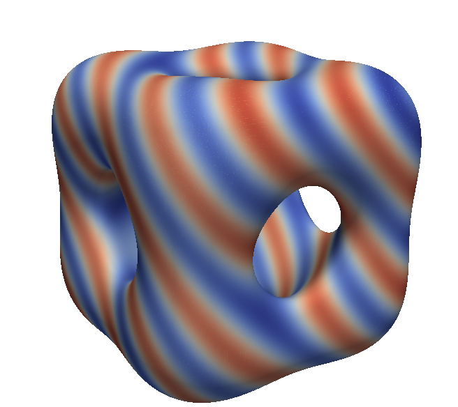
Figure 1: Computational results from Example 3: $u_{h}$ plotted on the zero level surface of $I_{h}\phi$. Colouring ranges from the minimum -86.45 to the maximum 99.57 of the solution.

4.1 Results using piecewise quadratic finite elements

Even though we have restricted our error analysis to the case of piecewise linear finite elements it is not difficult to apply our approach to quadratic elements. In order to do so, we use

$$\widetilde{V}_{h}:=\left\{v_{h}\in C(D_{h}):v_{h}\mbox{ is quadratic on }T\mbox{ for all }T\in\widetilde{\mathcal{T}}_{h}\right\}$$ (4.1)

instead of (2.33) and define the forms $a_{h}$ and $l_{h}$ (for the case $a_{ij}=\delta_{ij},a_{0}=1$) by

$$a_{h}(v_{1},v_{2}) := \varepsilon^{-1}\sum_{T\in\widetilde{\mathcal{T}}_{h}}Q_{T}\left[\varrho\,\nabla v_{1}\cdot\nabla v_{2}\,|\nabla I_{h}\phi|+\varrho\,v_{1}\,v_{2}\,|\nabla I_{h}\phi|\right]$$

$$l_{h}(v) := \varepsilon^{-1}\sum_{T\in\widetilde{\mathcal{T}}_{h}}Q_{T}\left[\varrho\,I_{h}\widehat{f}\,v\,|\nabla I_{h}\phi|\right],$$

where $I_{h}$ denotes the Lagrange interpolation operator for piecewise quadratic finite elements. The results in Table 5 correspond to the setting outlined in Example 1. Using a quadrature rule of order $q=6$ we see eocs close to order four for $\mathcal{E}_{2}$ and $\mathcal{E}_{4}$ in contrast to the eocs close to order two, that are displayed in Table 2, for the corresponding affine finite element approximation. The fact that the eocs for $\mathcal{E}_{1}$ and $\mathcal{E}_{3}$ are close to four (rather than six as expected for quadratic elements) is a consequence of the term $\varepsilon^{2}=\gamma^{2}h^{2}$ in (2.39) which now dominates.

$h$	$\varepsilon$	$\mathcal{E}_{1}$	$eoc_{1}$	$\mathcal{E}_{2}$	$eoc_{2}$	$\mathcal{E}_{3}$	$eoc_{3}$	$\mathcal{E}_{4}$	$eoc_{4}$
1.875e-02	$0.2$	2.378e-06	-	6.876e-05	-	7.063e-06	-	3.495e-08	-
9.375e-03	$0.1$	1.471e-07	4.01	4.265e-06	4.01	4.445e-07	3.99	1.913e-09	4.19
4.687e-03	$0.05$	9.169e-09	4.00	2.661e-07	4.00	2.783e-08	4.00	1.289e-10	3.89
2.344e-03	$0.025$	5.727e-10	4.00	1.663e-08	4.00	1.740e-09	4.00	7.712e-12	4.06
1.172e-03	$0.0125$	3.579e-11	4.00	1.043e-09	3.99	1.088e-10	4.00	4.825e-13	4.00

Table 5: Errors and experimental orders of convergence for Example 1, using $(\ref{Vrq})$ with $q=6$

Acknowledgements
VS would like to thank the Isaac Newton Institute for Mathematical Sciences for support and hospitality during the programme Geometry, compatibility and structure preservation in computational differential equations when work on this paper was undertaken. This work was supported by: EPSRC grant number EP/R014604/1.

Appendix A Appendix

The aim of this appendix is to derive certain properties of the projection $p$ and the extension $u^{e}(x)=u(p(x))$ which have been used in the analysis above. To begin, we infer from the definition of $u^{e}$ for $1\leq i,j\leq n+1$ that

$$u^{e}_{x_{i}}(x) = \sum_{k=1}^{n+1}\underline{D}_{k}u(p(x))\,p_{k,x_{i}}(x);$$ (A.1)

$$u^{e}_{x_{i}x_{j}}(x) = \sum_{k,l=1}^{n+1}\underline{D}_{l}\,\underline{D}_{k}u(p(x))\,p_{k,x_{i}}(x)\,p_{l,x_{j}}(x)+\sum_{k=1}^{n+1}\underline{D}_{k}u(p(x))\,p_{k,x_{i}x_{j}}(x).$$ (A.2)

Lemma. A.1.

Let $k\in\{0,1,2\}$ and $u\in H^{k}(\Gamma)$. Then

$$|u^{e}|_{H^{k}(U_{r})}\leq C\sqrt{r}\|u\|_{H^{k}(\Gamma)},\quad 0<r<\delta.$$ (A.3)

Proof. Using the transformation $F:\Gamma\times(-r,r)\rightarrow U_{r}$ with Jacobian determinant $\mu$, (A.1), (A.2) and the fact that $p\in C^{2}$ we obtain

$$|u^{e}|_{H^{k}(U_{r})}^{2}=\sum_{|\beta|=k}\int_{U_{r}}|D^{\beta}u^{e}(x)|^{2}\,{\rm d}x\leq C\,\sum_{|\kappa|=0}^{|\beta|}\int_{-r}^{r}\int_{\Gamma}|D^{\kappa}_{\Gamma}\,u(p)|^{2}\,\mu(p,s)\,{\rm d}S_{p}\;{\rm d}s\leq C\,r\,\|u\|_{H^{k}(\Gamma)}^{2}$$

and the result follows.      

In order to obtain more precise information about $p$ and its derivatives we essentially follow the argument in [9, Section 2.1], where the corresponding formulae were derived for the case $A=I$. For $x\in U_{\delta}$, we consider the function

$$\eta_{x}(\tau):=F(p(x),(1-\tau)\phi(x))=\gamma_{p(x)}((1-\tau)\phi(x)),\quad\tau\in[0,1],$$

where $\gamma_{p}$ was defined in (2.11). Since $p\in C^{2}$, it follows that $(x,\tau)\mapsto\eta_{x}(\tau)$ has continuous partial derivatives of second order with respect to $x$. Clearly, $\eta_{x}(1)=F(p(x),0)=p(x),\eta_{x}(0)=F(p(x),\phi(x))=x$. Furthermore, we infer from (2.11) that for $k=1,\ldots,n+1$

$$\eta_{x,k}^{\prime}(\tau)=-\phi(x)\,\gamma_{p(x),k}^{\prime}((1-\tau)\phi(x))=-\phi(x)\,\frac{1}{z_{x}(\tau)}\sum_{l=1}^{n+1}a_{kl}(p(x))\phi_{x_{l}}(\eta_{x}(\tau)),$$ (A.4)

where $z_{x}(\tau)=\sum_{r,s=1}^{n+1}a_{rs}(p(x))\phi_{x_{r}}(\eta_{x}(\tau))\phi_{x_{s}}(\eta_{x}(\tau))$. Let us abbreviate $w(x):=z_{x}(0)$. The following relations will help to simplify some of the subsequent calculations.

Lemma. A.2.

There exist $d^{A}_{k},d^{w}\in C^{2}$ such that

$$\sum_{l=1}^{n+1}a_{kl}(p(x))\phi_{x_{l}}(x) = \phi_{x_{k}}(x)+\phi(x)d^{A}_{k}(x),$$ (A.5)

$$w(x) = |\nabla\phi(x)|^{2}+\phi(x)d^{w}(x).$$ (A.6)

Furthermore, if $f:\Gamma\rightarrow\mathbb{R}$ is differentiable, then there are $d^{f}_{k}\in C^{2}$ such that

$$\sum_{k=1}^{n+1}\underline{D}_{k}f(p(x))\phi_{x_{k}}(x)=\phi(x)\,\sum_{k=1}^{n+1}\underline{D}_{k}f(p(x))d_{k}^{f}(x).$$ (A.7)

Proof. Recalling that $A(p)\nu(p)=\nu(p),\,p\in\Gamma$ as well as $\eta_{x}(0)=x,\eta_{x}(1)=p(x)$ we obtain with the help of (A.4)

$$\sum_{l=1}^{n+1}a_{kl}(p(x))\phi_{x_{l}}(x)=\phi_{x_{k}}(p(x))+\sum_{l=1}^{n+1}a_{kl}(p(x))\bigl{(}\phi_{x_{l}}(x)-\phi_{x_{l}}(p(x))\bigr{)}$$ (A.8)

$$= \phi_{x_{k}}(x)-\sum_{l=1}^{n+1}\bigl{(}a_{kl}(p(x))-\delta_{kl}\bigr{)}\bigl{(}\phi_{x_{l}}(\eta_{x}(1))-\phi_{x_{l}}(\eta_{x}(0))\bigr{)}$$

$$= \phi_{x_{k}}(x)+\phi(x)d^{A}_{k}(x).$$

Note that $d^{A}_{k}\in C^{2}$, since this is true for $x\mapsto\eta_{x}$ and $x\mapsto a_{kl}(p(x))$. The relation (A.6) immediately follows from (A.5). Next, observing that $\nabla_{\Gamma}f(p(x))\in T_{p(x)}\Gamma$ and $\nabla\phi(p(x))\perp T_{p(x)}\Gamma$ we infer that

$$\sum_{k=1}^{n+1}\underline{D}_{k}f(p(x))\,\phi_{x_{k}}(x)=\sum_{k=1}^{n+1}\underline{D}_{k}f(p(x))\bigl{(}\phi_{x_{k}}(x)-\phi_{x_{k}}(p(x))\bigr{)},$$

which implies (A.7) in a similar way as above.      

Inserting (A.5) and (A.6) into (A.4) we infer that there exist $d^{\eta,1}_{k}\in C^{2}$ such that

$$\eta_{x,k}^{\prime}(0)=-\frac{\phi(x)\phi_{x_{k}}(x)}{|\nabla\phi(x)|^{2}}+\phi(x)^{2}d^{\eta,1}_{k}(x),\quad 1\leq k\leq n+1.$$ (A.9)

If we differentiate (A.4) and use again (A.4) we obtain

$$\eta_{x,k}^{\prime\prime}(\tau)=-\frac{\phi(x)}{z_{x}(\tau)}\sum_{l,m=1}^{n+1}a_{kl}(p(x))\phi_{x_{l}x_{m}}(\eta_{x}(\tau))\eta_{x,m}^{\prime}(\tau)+\frac{\phi(x)}{z_{x}(\tau)^{2}}z_{x}^{\prime}(\tau)\sum_{l=1}^{n+1}a_{kl}(p(x))\phi_{x_{l}}(\eta_{x}(\tau))$$

$$= \frac{\phi(x)^{2}}{z_{x}(\tau)^{2}}\sum_{l,m,q=1}^{n+1}a_{kl}(p(x))a_{mq}(p(x))\phi_{x_{l}x_{m}}(\eta_{x}(\tau))\phi_{x_{q}}(\eta_{x}(\tau))$$

$$-2\frac{\phi(x)^{2}}{z_{x}(\tau)^{2}}\sum_{l,m,q,r,s=1}^{n+1}a_{kl}(p(x))a_{mq}(p(x))a_{rs}(p(x))\phi_{x_{r}x_{m}}(\eta_{x}(\tau))\phi_{x_{l}}(\eta_{x}(\tau))\phi_{x_{q}}(\eta_{x}(\tau))\phi_{x_{s}}(\eta_{x}(\tau)).$$

Taylor’s theorem together with (A.9) and (A) implies the existence of $d^{p,0}_{k}\in C^{2}$ with

$$p_{k}(x) = \eta_{x,k}(1)=\eta_{x,k}(0)+\eta_{x,k}^{\prime}(0)+\int_{0}^{1}(1-\tau)\eta_{x,k}^{\prime\prime}(\tau)d\tau$$ (A.11)

$$= x_{k}-\frac{\phi(x)\phi_{x_{k}}(x)}{|\nabla\phi(x)|^{2}}+\phi(x)^{2}d^{p,0}_{k}(x).$$

The relation (A.11) allows us to prove a bound between $p(x)$ and the closest-point projection $\widehat{p}(x)$, which is used in the error analysis.

Lemma. A.3.

There exists a constant $C$ such that

$$|p(x)-\widehat{p}(x)|\leq C\,\phi(x)^{2}\qquad\forall\ x\in U_{\delta}.$$ (A.12)

Proof. Let us fix $x\in U_{\delta}$. Using (A.11) and the fact that $p(x)\in\Gamma$ we have

$$|x-\widehat{p}(x)|\leq|x-p(x)|\leq C|\phi(x)|.$$

Furthermore, since $T_{\widehat{p}(x)}\Gamma=\mbox{span}\{\nabla\phi(\widehat{p}(x))\}^{\perp}$, (2.1) implies that there exists $\lambda\in\mathbb{R}$ such that $x-\widehat{p}(x)=\lambda\,\nabla\phi(\widehat{p}(x))$. Taylor expansion around $\widehat{p}(x)$ yields together with $\phi(\widehat{p}(x))=0$, that

$$\phi(x) = \nabla\phi(\widehat{p}(x))\cdot(x-\widehat{p}(x))+\frac{1}{2}(x-\widehat{p}(x))^{t}D^{2}\phi(\xi)(x-\widehat{p}(x))$$

$$= \lambda\,|\nabla\phi(\widehat{p}(x))|^{2}+\frac{1}{2}(x-\widehat{p}(x))^{t}D^{2}\phi(\xi)(x-\widehat{p}(x))$$

for some $\xi\in[\widehat{p}(x),x]$. Thus

$$\lambda=\frac{\phi(x)}{|\nabla\phi(\widehat{p}(x))|^{2}}+r,\quad\mbox{ where }|r|\leq C|x-\widehat{p}(x)|^{2}\leq C\phi(x)^{2}$$

and therefore

$$x-\widehat{p}(x)=\phi(x)\,\frac{\nabla\phi(\widehat{p}(x))}{|\nabla\phi(\widehat{p}(x))|^{2}}+r\,\nabla\phi(\widehat{p}(x)).$$ (A.13)

If we combine this relation with (A.11) we find that

$$p(x)-\widehat{p}(x)=\phi(x)\left[\frac{\nabla\phi(\widehat{p}(x))}{|\nabla\phi(\widehat{p}(x))|^{2}}-\frac{\nabla\phi(x)}{|\nabla\phi(x)|^{2}}\right]+r\nabla\phi(\widehat{p}(x))+\phi(x)^{2}\,d^{p,0}(x),$$

from which we deduce (A.12), since $|x-\widehat{p}(x)|\leq C\,|\phi(x)|$ and $|r|\leq C\phi(x)^{2}$.      

Our next aim is to improve on (A.11) by using a Taylor expansion of one degree higher. We deduce from (A), (A.5) and (A.6) that

$$\eta_{x,k}^{\prime\prime}(0) = \frac{\phi(x)^{2}}{w(x)^{2}}\sum_{l,m,q=1}^{n+1}a_{kl}(p(x))a_{mq}(p(x))\phi_{x_{l}x_{m}}(x)\phi_{x_{q}}(x)$$ (A.14)

$$-2\frac{\phi(x)^{2}}{w(x)^{2}}\sum_{l,m,q,r,s=1}^{n+1}a_{kl}(p(x))a_{mq}(p(x))a_{rs}(p(x))\phi_{x_{r}x_{m}}(x)\phi_{x_{l}}(x)\phi_{x_{q}}(x)\phi_{x_{s}}(x)$$

$$= \frac{\phi(x)^{2}}{|\nabla\phi(x)|^{4}}\sum_{l,m=1}^{n+1}a_{kl}(p(x))\phi_{x_{l}x_{m}}(x)\phi_{x_{m}}(x)$$

$$-2\frac{\phi(x)^{2}\phi_{x_{k}}(x)}{|\nabla\phi(x)|^{4}}\sum_{m,r=1}^{n+1}\phi_{x_{r}}(x)\phi_{x_{m}}(x)\phi_{x_{r}x_{m}}(x)+\phi(x)^{3}\,d^{\eta,2}_{k}(x),$$

where $d^{\eta,2}_{k}\in C^{2}$. Differentiating (A) and using (A.4) as well as (A.14) we obtain

$$p_{k}(x) = \eta_{x,k}(1)=\eta_{x,k}(0)+\eta_{x,k}^{\prime}(0)+\frac{1}{2}\,\eta_{x,k}^{\prime\prime}(0)+\frac{1}{2}\int_{0}^{1}(1-\tau)^{2}\eta_{x,k}^{\prime\prime\prime}(\tau)d\tau$$ (A.15)

$$= x_{k}-\frac{\phi(x)}{w(x)}\,\sum_{l=1}^{n+1}a_{kl}(p(x))\,\phi_{x_{l}}(x)+\frac{1}{2}\frac{\phi(x)^{2}}{|\nabla\phi(x)|^{4}}\sum_{l,m=1}^{m+1}a_{kl}(p(x))\phi_{x_{l}x_{m}}(x)\phi_{x_{m}}(x)$$

$$-\frac{\phi(x)^{2}\phi_{x_{k}}(x)}{|\nabla\phi(x)|^{4}}\sum_{m,r=1}^{n+1}\phi_{x_{r}}(x)\phi_{x_{m}}(x)\phi_{x_{r}x_{m}}(x)+\phi(x)^{3}\,\tilde{d}^{p,0}_{k}(x),$$

where $\tilde{d}^{p,0}_{k}\in C^{2}$.
Before we continue let us remark that we may deduce from (A.11)

$$p_{k,x_{i}}(x)=\delta_{ik}-\frac{\phi_{x_{i}}(x)\phi_{x_{k}}(x)}{|\nabla\phi(x)|^{2}}+\phi(x)d^{p,1}_{ik}(x),\quad 1\leq i,k\leq n+1,$$ (A.16)

where $d^{p,1}_{ik}\in C^{1}$. Combining this relation with (A.7) we obtain

$$\frac{\partial}{\partial x_{i}}[a_{kl}(p(x))]=\sum_{m=1}^{n+1}\underline{D}_{m}a_{kl}(p(x))p_{m,x_{i}}(x)$$ (A.17)

$$= \underline{D}_{i}a_{kl}(p(x))-\sum_{m=1}^{n+1}\underline{D}_{m}a_{kl}(p(x))\frac{\phi_{x_{i}}(x)\phi_{x_{m}}(x)}{|\nabla\phi(x)|^{2}}+\phi(x)\sum_{m=1}^{n+1}\underline{D}_{m}a_{kl}(p(x))d^{p,1}_{im}(x)$$

$$= \underline{D}_{i}a_{kl}(p(x))+\phi(x)d^{A,i}_{kl}(x),$$

where $d^{A,i}_{kl}\in C^{1}$. Differentiating (A.15) with respect to $x_{i}$ and using (A.17), (A.6) we deduce for $1\leq i,k\leq n+1$

$$p_{k,x_{i}}(x) = \delta_{ik}-\frac{\phi_{x_{i}}(x)}{w(x)}\sum_{l=1}^{n+1}a_{kl}(p(x))\phi_{x_{l}}(x)+\phi(x)\frac{\phi_{x_{k}}(x)w_{x_{i}}(x)}{|\nabla\phi(x)|^{4}}-\phi(x)\sum_{l=1}^{n+1}\frac{\underline{D}_{i}a_{kl}(p(x))\phi_{x_{l}}(x)}{|\nabla\phi(x)|^{2}}$$ (A.18)

$$-\phi(x)\sum_{l=1}^{n+1}\frac{a_{kl}(p(x))\phi_{x_{l}x_{i}}(x)}{|\nabla\phi(x)|^{2}}+\frac{\phi(x)\phi_{x_{i}}(x)}{|\nabla\phi(x)|^{4}}\sum_{l,m=1}^{m+1}a_{kl}(p(x))\phi_{x_{l}x_{m}}(x)\phi_{x_{m}}(x)$$

$$-2\frac{\phi(x)\phi_{x_{i}}(x)\phi_{x_{k}}(x)}{|\nabla\phi(x)|^{4}}\sum_{m,r=1}^{n+1}\phi_{x_{r}}(x)\phi_{x_{m}}(x)\phi_{x_{r}x_{m}}(x)+\phi(x)^{2}\tilde{d}^{p,1}_{ik}(x),$$

where $\tilde{d}^{p,1}_{ik}\in C^{1}$. If we differentiate this relation with respect to $x_{j}$ and use (A.5), (A.17) we infer for $1\leq i,j,k\leq n+1$

$$p_{k,x_{i}x_{j}}(x)=-\sum_{l=1}^{n+1}\left\{\frac{\underline{D}_{j}a_{kl}(p(x))\phi_{x_{i}}(x)\phi_{x_{l}}(x)}{|\nabla\phi(x)|^{2}}+\frac{\underline{D}_{i}a_{kl}(p(x))\phi_{x_{j}}(x)\phi_{x_{l}}(x)}{|\nabla\phi(x)|^{2}}\right\}$$ (A.19)

$$-\sum_{l=1}^{n+1}\left\{\frac{a_{kl}(p(x))\phi_{x_{i}}(x)\phi_{x_{l}x_{j}}(x)}{|\nabla\phi(x)|^{2}}+\frac{a_{kl}(p(x))\phi_{x_{j}}(x)\phi_{x_{l}x_{i}}(x)}{|\nabla\phi(x)|^{2}}\right\}$$

$$+\sum_{l,m=1}^{n+1}\frac{a_{kl}(p(x))\phi_{x_{i}}(x)\phi_{x_{j}}(x)\phi_{x_{m}}(x)\phi_{x_{l}x_{m}}(x)}{|\nabla\phi(x)|^{4}}$$

$$+\beta_{ijk}(x)\phi_{x_{k}}(x)+\phi(x)\,\tilde{d}^{p,2}_{ijk}(x)+\phi(x)^{2}\,\tilde{d}^{p,3}_{ijk}(x),$$

where $\beta_{ijk},\tilde{d}^{p,2}_{ij}\in C^{1},\tilde{d}^{p,3}_{ijk}\in C^{0}$. Using the above formulae we now obtain:

Lemma. A.4.

Suppose that $u:\Gamma\rightarrow\mathbb{R}$ is a solution of (2.3). Then, $u^{e}$ satisfies (2.16), (2.17).

Proof. Combining (A.1), (A.16) and (A.7) we deduce that

$$u^{e}_{x_{i}}(x)=\sum_{k=1}^{n+1}\underline{D}_{k}u(p(x))\,p_{k,x_{i}}(x)=\underline{D}_{i}u(p(x))+\phi(x)\sum_{k=1}^{n+1}\alpha^{i}_{k}(x)\underline{D}_{k}u(p(x)),$$ (A.20)

where $\alpha^{i}_{k}\in C^{1}$. Similarly, using (A.2), (A.16), (A.19) and (A.7) we obtain

$$u^{e}_{x_{i}x_{j}}(x) = \sum_{k,l=1}^{n+1}\underline{D}_{l}\underline{D}_{k}u(p(x))p_{k,x_{i}}(x)p_{l,x_{j}}(x)+\sum_{k=1}^{n+1}\underline{D}_{k}u(p(x))p_{k,x_{i}x_{j}}(x)$$ (A.21)

$$= \sum_{k=1}^{n+1}\underline{D}_{j}\underline{D}_{k}u(p(x))\bigl{(}\delta_{ik}-\frac{\phi_{x_{i}}(x)\phi_{x_{k}}(x)}{|\nabla\phi(x)|^{2}}\bigr{)}$$

$$-\sum_{k,l=1}^{n+1}\underline{D}_{k}u(p(x))\left\{\frac{\underline{D}_{j}a_{kl}(p(x))\phi_{x_{i}}(x)\phi_{x_{l}}(x)}{|\nabla\phi(x)|^{2}}+\frac{\underline{D}_{i}a_{kl}(p(x))\phi_{x_{j}}(x)\phi_{x_{l}}(x)}{|\nabla\phi(x)|^{2}}\right\}$$

$$-\sum_{k,l=1}^{n+1}\underline{D}_{k}u(p(x))\left\{\frac{a_{kl}(p(x))\phi_{x_{i}}(x)\phi_{x_{l}x_{j}}(x)}{|\nabla\phi(x)|^{2}}+\frac{a_{kl}(p(x))\phi_{x_{j}}(x)\phi_{x_{l}x_{i}}(x)}{|\nabla\phi(x)|^{2}}\right\}$$

$$+\sum_{k,l,m=1}^{n+1}\underline{D}_{k}u(p(x))\frac{a_{kl}(p(x))\phi_{x_{i}}(x)\phi_{x_{j}}(x)\phi_{x_{m}}(x)\phi_{x_{l}x_{m}}(x)}{|\nabla\phi(x)|^{4}}$$

$$+\sum_{1\leq|\kappa|\leq 2}\bigl{(}\phi(x)\alpha^{ij}_{\kappa}(x)+\phi(x)^{2}\tilde{\alpha}^{ij}_{\kappa}(x)\bigr{)}D_{\Gamma}^{\kappa}u(p(x)),$$

where $\alpha^{ij}_{\kappa}\in C^{1},\tilde{\alpha}^{ij}_{\kappa}\in C^{0}$. Recalling (A.5) and using (A.21) and the symmetry of the coefficients $a_{ij}$ we infer that

$$\sum_{i,j=1}^{n+1}a_{ij}^{e}(x)\,u^{e}_{x_{i}x_{j}}(x)=\sum_{i,j=1}^{n+1}a_{ij}(p(x))\,u^{e}_{x_{i}x_{j}}(x)$$ (A.22)

$$= \sum_{i,j=1}^{n+1}a_{ij}(p(x))\underline{D}_{j}\underline{D}_{i}u(p(x))-\sum_{j,k=1}^{n+1}\underline{D}_{j}\underline{D}_{k}u(p(x))\,\frac{\phi_{x_{j}}(x)\phi_{x_{k}}(x)}{|\nabla\phi(x)|^{2}}$$

$$-2\sum_{j,k,l=1}^{n+1}\underline{D}_{k}u(p(x))\underline{D}_{j}a_{kl}(p(x))\frac{\phi_{x_{j}}(x)\phi_{x_{l}}(x)}{|\nabla\phi(x)|^{2}}-\sum_{k,l,m=1}^{n+1}a_{kl}(p(x))\underline{D}_{k}u(p(x))\frac{\phi_{x_{m}}(x)\phi_{x_{l}x_{m}}(x)}{|\nabla\phi(x)|^{2}}$$

$$+\sum_{1\leq|\kappa|\leq 2}\bigl{(}\phi(x)\beta_{\kappa}(x)+\phi(x)^{2}\tilde{\beta}_{\kappa}(x)\bigr{)}D_{\Gamma}^{\kappa}u(p(x))$$

$$= \sum_{i,j=1}^{n+1}a_{ij}(p(x))\underline{D}_{j}\underline{D}_{i}u(p(x))-\sum_{k,l,m=1}^{n+1}a_{kl}(p(x))\underline{D}_{k}u(p(x))\frac{\phi_{x_{m}}(x)\phi_{x_{l}x_{m}}(x)}{|\nabla\phi(x)|^{2}}$$

$$+\sum_{1\leq|\kappa|\leq 2}\bigl{(}\phi(x)\gamma_{\kappa}(x)+\phi(x)^{2}\tilde{\gamma}_{\kappa}(x)\bigr{)}D_{\Gamma}^{\kappa}u(p(x)),$$

where the last identity follows from (A.7) and where $\gamma_{\kappa}\in C^{1},\tilde{\gamma}_{\kappa}\in C^{0}$. On the other hand, (A.17) and (A.20) yield

$$\sum_{i,j=1}^{n+1}a^{e}_{ij,x_{j}}(x)u^{e}_{x_{i}}(x)=\sum_{i,j=1}^{n+1}\underline{D}_{j}a_{ij}(p(x))\,\underline{D}_{i}u(p(x))+\phi(x)\sum_{k=1}^{n+1}\tilde{\beta}_{k}(x)\underline{D}_{k}u(p(x)),$$ (A.23)

where $\tilde{\beta}_{k}\in C^{1}$. Combining (A.22) and (A.23) we find that

$$\frac{1}{|\nabla\phi(x)|}\nabla\cdot\left(A^{e}(x)\nabla u^{e}(x)|\nabla\phi(x)|\right)$$

$$= \sum_{i,j=1}^{n+1}\bigl{(}a^{e}_{ij,x_{j}}(x)u^{e}_{x_{i}}(x)+a^{e}_{ij}(x)u^{e}_{x_{i}x_{j}}(x)\bigr{)}+\frac{1}{|\nabla\phi(x)|^{2}}\sum_{i,j,k=1}^{n+1}a^{e}_{ij}(x)u^{e}_{x_{i}}(x)\phi_{x_{k}}(x)\phi_{x_{k}x_{j}}(x)$$

$$= \sum_{i,j=1}^{n+1}\underline{D}_{j}\bigl{(}a_{ij}(p(x))\underline{D}_{i}u(p(x))\bigr{)}+\sum_{1\leq|\kappa|\leq 2}\bigl{(}\phi(x)b_{\kappa}(x)+\phi(x)^{2}c_{\kappa}(x)\bigr{)}D_{\Gamma}^{\kappa}u(p(x)),$$

where $b_{\kappa}\in C^{1},c_{\kappa}\in C^{0}$. Combining this relation with (2.3) implies (2.16) and (2.17).

References

• [1] Barrett, J.W and Nürnberg, R. and Styles, V.: Finite element approximation of a phase field model for void electromigration. SIAM J. Numer. Anal. 46, 738–772 (2004).
• [2] Bertalmio, M., Cheng, L.T., Osher, S., Sapiro, G.: Variational problems and partial differential equations on implicit surfaces: The framework and examples in image processing and pattern formation. J. Comput. Phys. 174, 759–780 (2001).
• [3] Bonito, A., Demlow, A., Nochetto, R.H.: Finite element methods for the Laplace-Beltrami operator. Handbook of Numerical Analysis, vol. XXI, Geometric Partial Differential Equations - Part 1 (2020).
• [4] Burger, M: Finite element approximation of elliptic partial differential equations on implicit surfaces. Comput. Vis. Sci. 12, 87–100 (2009).
• [5] Burman, E., Hansbo, P., Larson, M.G.: A stabilized cut finite element method for partial differential equations on surfaces: The Laplace–Beltrami operator. Comput. Methods Appl. Mech. Engrg. 285, 188-–207 (2015).
• [6] Burman, E., Hansbo, P., Larson, M.G., Massing, A., Zahedi, S.: Full gradient stabilized cut finite element methods for surface partial differential equations. Comput. Methods Appl. Mech. Engrg. 310, 278-–296 (2016).
• [7] Chernyshenko, A.Y, Olshanskii, M.A.: Non-degenerate Eulerian finite element method for solving PDEs on surfaces. Russian J. Numer. Anal. Math. Modelling 28, no. 2, 101-–124 (2013).
• [8] Deckelnick, K., Dziuk, G., Elliott, C.M., Heine, C.-J.: An h-narrow band finite-element method for elliptic equations on implicit surfaces. IMA J. Numer. Anal. 30, 351–376 (2010).
• [9] Deckelnick, K., Elliott, C.M., Ranner, T.: Unfitted finite element methods using bulk meshes fur surface partial differential equations. SIAM J. Numer. Anal. 52, 2137–2162 (2014).
• [10] Deckelnick, K., Styles, V.: Stability and error analysis for a diffuse interface approach to an advection-diffusion equation on a moving surface. Numer. Math. 139, 709–741 (2018).
• [11] Demlow, A.: Higher-order finite element methods and pointwise error estimates for elliptic problems on surfaces. SIAM J. Numer. Anal. 47, no. 2, 805-–827 (2009).
• [12] Demlow, A., Dziuk, G.: An adaptive finite element method for the Laplace–Beltrami operator on implicitly defined surfaces. SIAM J. Numer. Anal. 45, 421–442 (2007).
• [13] Demlow, A., Olshanskii, M.A.: An adaptive surface finite element method based on volume meshes. SIAM J. Numer. Anal. 50, no. 3, 1624–-1647 (2012).
• [14] Dziuk, G.: Finite elements for the Beltrami operator on arbitrary surfaces. In: Partial differential equations and calculus of variations, S. Hildebrandt and R. Leis, eds., vol. 1357 of Lecture Notes in Mathematics, Springer-Verlag, Berlin, 1988, pp. 142–155.
• [15] Dziuk, G., Elliott, C.M.: Finite element methods for surface PDEs. Acta Numer. 22, 289–396 (2013).
• [16] Elliott, C.M., Stinner, B.: Analysis of a diffuse interface approach to an advection diffusion equation on a moving surface. Math. Models Methods Appl. Sci. 19, 787–802 (2009).
• [17] Elliott, C.M., Stinner, B., Styles, V., Welford, R.: Numerical computation of advection and diffusion on evolving diffuse interfaces. IMA J. Numer. Anal. 31, 786–812 (2011).
• [18] Elliott, C.M., Ranner, T.: Finite element analysis for a coupled bulk–surface partial differential equation. IMA J. Numer. Anal. 33, 377–402 (2013).
• [19] Gilbarg, D., Trudinger, N.S.: Elliptic Partial Differential Equations of Second Order, Springer–Verlag, Berlin, 2nd ed., 1988.
• [20] Grande, J., Lehrenfeld, C., Reusken, A.: Analysis of a high-order trace finite element method for PDEs on level set surfaces. SIAM J. Numer. Anal. 56, 228–255 (2018).
• [21] Hansbo, A., Hansbo, P.: An unfitted finite element method, based on Nitsche’s method, for elliptic interface problems. Comput. Methods Appl. Mech. Engrg. 191, 5537–5552 (2002).
• [22] Hansbo, A., Hansbo, P.: A finite element method for the simulation of strong and weak discontinuities in solid mechanics. Comput. Methods Appl. Mech. Engrg. 193, 3523–3540 (2004).
• [23] Macdonald, C.B., Ruuth, S.J.: The Implicit Closest Point Method for the Numerical Solution of Partial Differential Equations on Surfaces. SIAM J. Sci. Comput. 31, 4330-–4350 (2009).
• [24] Olshanskii, M.A., Reusken, A.: A finite element method for surface PDEs: matrix properties. Numer. Math. 114, no. 3, 491–-520 (2010).
• [25] Olshanskii, M.A., Reusken, A., Grande, J.: A finite element method for elliptic equations on surfaces. SIAM J. Numer. Anal. 47, no. 5, 3339-–3358 (2009).
• [26] Olshanskii, M.A., Safin, D.: A narrow-band unfitted finite element method for elliptic PDEs posed on surfaces. Math. Comp. 85, no. 300, 1549–1570 (2016).
• [27] Rätz, A., Voigt, A.: PDE’s on surfaces - a diffuse interface approach. Comm. Math. Sci. 4, 575–590 (2006).
• [28] Reusken, A.: Analysis of trace finite element methods for surface partial differential equations. IMA J. Numer. Anal. 35, no. 4, 1568–-1590 (2015).
• [29] Schmidt, A. and Siebert, K.G.: Design of adaptive finite element software. The finite element toolbox ALBERTA. Lecture Notes in Computational Science and Engineering 42, Springer-Verlag, Berlin, (2005).