Radial Distributions of Coronal Electron Temperatures: specificities of the DYN model

1 Introduction and setting the stage for DYN model

S-Introduction

Measurements of White Light (WL) brightnesses and polarization (pB) during solar eclipses have often been used in the past to infer and calculate the electron density distribution ($\mathrm{n_{e}}$), the radial distribution of coronal electrons densities, or of the hypothetic Coronium atomic element.

According to Baumbach (1937) pioneering analysis of coronal WL brightnesses, $\mathrm{n_{e}(r)}$ can best be approximated by a sum of terms inversely proportional powers of the r, the radial distance from the solar center. This finding is at odds with the standard exponential decreases, generally postulated for density profiles in stellar and planetary atmospheres, at this epoch.

Using Baumbach’s empirical formula for fitting observed coronal densities distributions, and assuming cylindrical symmetry of the corona around the Sun’s axis of rotation, Saito (1970, hereafter S70) constructed a two-dimensional model for $\mathrm{n_{e}(r,\phi)}$ as a function of r, and heliospheric latitude, $\mathrm{\phi}$. Their empirical 2D-model is based on a series of available eclipse observations corresponding to epochs of minimum solar activity. Saito ’s empirical coronal electron density 2D-model became popular, and has been adopted in many studies of the solar corona as well as in the present one, although its range of application is restricted to r $<$ 4 $\mathrm{R_{S}}$ because of signal-to-noise (S/N) issues related to the WL coronal brightnesses beyond this distance.

In order to extend S70’s density distributions up to the Earth’s orbit and beyond, Lemaire and Stegen (2016) added an extra-term inversely proportional to the square of r. This additional power law term fits well the solar wind distribution, whose electron density and bulk velocity at 1 AU, will be input parameters designed hereafter by $\mathrm{n_{E}}$ and $\mathrm{u_{E}}$, respectively. Typical values of these input parameters for $\mathrm{n_{e}(r,\phi)}$, will be chosen within the ranges of SW observations reported by Ebert et al. (2009). The table 1 in Lemaire and Stegen (2016) contains the values of these inputs for a set of DYN models illustrated and discussed in the present paper, as well as in the previous one.

The analytical expression of S70’s extended density distributions (in electrons / $\mathrm{cm^{3}}$) employed to determine the temperature distributions for all DYN models is recalled here:

$$\ilabel{ne}\begin{aligned} n_{e}(r,\phi)=10^{8}\ [3.09\ r^{-16}\ (1-0.5\sin\phi)+1.58\ r^{-6}\ (1-0.95\sin\phi)+\\ 0.0251\ r^{-2.5}\ (1-\sqrt{\sin\phi})]+n_{E}\ (215/r)^{2},\end{aligned}$$ (1)

where 1 AU is assumed to be 215 $\mathrm{R_{S}}$ and r is in units of $\mathrm{R_{S}}$.

A few typical density distributions derived from this formula are shown in figure F-density. In order to expand the inner and middle regions of the corona, where the greatest SW acceleration takes place, the logarithm of h, the altitude above the photosphere - normalised by the solar radius $\mathrm{R_{S}}$ - can be recommended for the horizontal axis, and has been used in all of our graphs.

The analytical expression (ne) happens to be a very convenient approximation in many respects.

1. First of all, it is most convenient to determine the radial distributions of the coronal density gradients, and therefore that of H, the electron density scale height. This enables the easy calculation of the radial profile of the scale-height temperature, hereafter labelled SHM temperature, because it is determined by the well-known Scale-Height-Method (SHM).

2. Furthermore, equation (ne) can be used to derive an analytical expression for the SW bulk velocity, u(r), by integrating the continuity equation - the conservation of the particle flux - from the Earth’s radial distance ($\mathrm{r_{E}}$) down to the base of the corona ($\mathrm{r_{b}}$), where $\mathrm{r_{b}}$ is defined hereafter to be at 1.003 $\mathrm{R_{S}}$.

   In the following DYN models this integration is performed along flow tubes whose geometrical cross-section, A(r), is an empirical function of r. The analytical formulas 10, 11, and 12 of Kopp and Holzer (1976) are used for A(r) (for more details see section 7 and the appendix of Lemaire and Stegen, 2016).

   The downward integration of the hydrodynamical continuity equation leads to an analytical expression for u(r) defined by:

   $$\ilabel{E-u}u(r,\phi)=u_{E}\frac{A_{E}}{A(r)}\frac{n_{E}}{n_{e}(r,\phi)},$$ (2)

   where $\mathrm{A_{E}}$ is the cross-section of the flow tube at 1 AU.

   To minimise the length of this paper, the mathematical formula used for A(r) will not be repeated here; it can be found in Lemaire and Stegen (2016), equation 12. Furthermore, we will restrict our DYN model calculations to spherical expansions of the SW, i.e. $\mathrm{A_{E}/A(r)}$ = (215/r)².

   We have assumed, like most other modellers of the SW that flow tubes of the plasma coincide with interplanetary magnetic flux tubes. This common assumption might be relaxed in the future, however, by implementing ad-hoc distributions of curl-free E-fields into the medium.

3. The analytical expressions ne and E-u allow the straightforward calculation of the radial gradient of the bulk velocity, u(r), as well as the dimensionless function F(r), corresponding to the ratio of the inertial force and the gravitation force acting on the expanding SW plasma.

   $$\ilabel{E-Fx}F(r)=\frac{1}{g_{S}R_{S}}\ r^{2}\ u(r)\ \frac{d[u(r)]}{dr},$$ (3)

   where $\mathrm{g_{S}}$ is the gravitational acceleration at the solar surface (274 m s^-2).

It can already be emphasized that the analytical distribution of u(r,$\phi$) provided by equation E-u is a continuous function of r, and most importantly, that this function has no point of singularity (saddle point) at the altitude where the radial expansion of the SW becomes supersonic. This key property constitutes a major difference between DYN models and the steady state hydrodynamical SW models where u(r) is a singular solution of the hydrodynamical moment/transport equations introduced by Parker (1958, 1963). This issue will be discussed in greater details in Section 6.

2 Temperature calculation by the DYN model

S-DYN-temperature

To obtain the radial distribution of the DYN temperature Lemaire and Stegen (2016) integrated the simplest approximation of hydrodynamic momentum transport equation, from infinity (where they assumed that the plasma temperature is equal to zero), down to $\mathrm{r_{b}}$, the base of the corona :

$$\ilabel{E-Te}T_{e}(r)=-\frac{T^{*}}{n_{e}(r)}\int_{\infty}^{r}\frac{n_{e}(r)}{r^{2}}\left[1+F(r)\right]dr,$$ (4)

where $\mathrm{T^{*}}$ is a normalisation temperature defined by equation 9 of Lemaire and Stegen (2016) (see also Alfvén, 1941). The value of $\mathrm{T^{*}}$ is proportional to the mass of the Sun, and inversely proportional to the solar radius. It is equal to 17 MK in all of the following applications.

A non-zero additive constant temperature, $\mathrm{T_{\infty}}$, corresponding to the actual electron temperature at the outer edge of the heliosphere could have been added to the right-hand-side of equation E-Te. However, the addition of a constant temperature of the order of 2000-3000 K does not change considerably the DYN temperature profile close to the Sun, indeed $\mathrm{T_{e}(r)}$ is orders of magnitude larger for $\mathrm{r_{b}<r<10~{}R_{S}}$ than $\mathrm{T_{\infty}}$. Therefore, it is not far from reality to set $\mathrm{T_{\infty}=0}$ as assumed in equation E-Te. We verified that the DYN temperatures profiles with two widely different values for $\mathrm{T_{\infty}}$ converge to the same temperatures for r $<$ 1.1 $\mathrm{R_{S}}$. This remarkable convergence of the DYN temperatures distributions at the base of the Corona, holds not only at equatorial latitudes but also over the poles.

In a next generation of our computer code we will start the numerical integration of equation E-Te at $\mathrm{r_{E}}$, where the SW electron temperature at 1AU, $\mathrm{T_{E}}$, will then be an input parameter of the DYN model, like $\mathrm{n_{E}}$ and $\mathrm{u_{E}}$. Ebert et al. (2009) is again a good source of typical $\mathrm{T_{E}}$ values that can then be used as a free input parameter in DYN calculations.

Let us re-emphasized that in the DYN model the boundary conditions are set in a large solar distance (i.e. 1 AU or infinity), and that the continuity and momentum equations are integrated downwards. This way DYN solutions deviate from the singular hydrodynamical solutions whose boundary conditions are set at the bottom of the corona, and for which the numerical integration is made upwards.

In section S-expansion we complete the work initiated in Lemaire and Stegen (2016) by analysing and discussing the properties of the DYN models for other sets of the $\mathrm{u_{E}}$ and $\mathrm{n_{E}}$ input parameters. Nevertheless, it is preferable to first present and discuss a few characteristic fits of the $\mathrm{n_{e}(r)}$ distribution (section S-Density) and some properties of the DYN temperature profiles (section S-Distributions).

3 Corona Electron Density Distributions inferred from eclipse observations.

S-Density

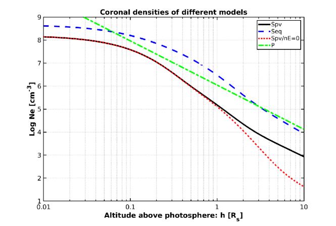
Figure 1.: Expanded coronal electron density distributions for the equatorial (blue-dashed curve, Seq), and polar regions described by Lemaire and Stegen (2016) (black curve, Spv), taken from S70 (red dotted curve, Spv/nE=0), and from Pottasch (1960) (green-dashed-dotted curve, P). Pottasch’s density distribution was also included in figure 6.5 of Parker (1963).F-density

The electron density distribution, $\mathrm{n_{e}(r)}$, implemented by different authors from eclipse observations is displayed in figure F-density. This graph is similar to the figure 1 of Lemaire and Stegen (2016) . It is included here for completion and easier access.

The black curve (Spv) corresponds to Saito’s polar density distribution which has been extended to large distances by adding the contribution of the Solar Wind density. The red-dotted curve (Spv/nE=0) is the same distribution but without the last term of equation (ne), i.e. without the contribution of the solar wind density. The DYN temperature determined for this (red) density distribution corresponds the HST temperature profile for which which u(r)= 0. Indeed, according to equation (E-u), u(r) is proportional to $\mathrm{n_{E}}$, thus u(r)=0 when $\mathrm{n_{E}}$=0. This (red) density profile can thus be viewed as a radial density distribution wherein the class of escaping SW particles would be missing in the exospheric coronal models of Lemaire and Scherer (1971, 1973).

In collisionless/kinetic models, it is exclusively the class of escaping electrons that contributes to the net outward flux of evaporating coronal electrons. The classes of ballistic and trapped particles don’t contribute to this net SW flux of particles. Indeed these latter electrons do not have sufficiently large energy to escape out Lemaire-Scherer’s electrostatic potential well. Nevertheless, they play a major role by contributing their electric charges to the total negative charge density of the coronal and SW plasma. Note also that these collisionless ballistic and trapped particles do not contribute either to the net outward flux of kinetic energy that is carried out of the corona into interplanetary space by the SW. Thus these low energy (sub-thermal and thermal) electrons contribute exclusively to the total negative charge density which must balance the positive charge density of the ions, in order to keep the plasma locally quasi-neutral. In contrast, in fluid or hydrodynamical representations of the coronal and SW plasma no such discrimination between sub-thermal and supra-thermal electrons, or between escaping, ballistic and trapped electrons is made explicitly. All classes of electrons are assumed to take part to the net outward fluxes of SW particles and of the SW kinetic energy. This constitutes a fundamental distinction between both types of plasma representations. These key differences are discussed in greater details in the review article by Echim, Lemaire, and Lie-Svendsen (2011).

The blue-dashed curve (Seq) corresponds to S70’s extended equatorial density model (i.e. for  $\mathrm{\phi}=0$). Note that the latter equatorial density (Seq) is significantly larger than the the polar density distribution (Spv) in the inner and middle corona.

The green curve (P) corresponds to a best fit of an equatorial electron density distribution during solar minimum determined by Pottasch (1960). It was derived from WL brightness and polarization measurements during the solar eclipse of 1952, under the assumption that the corona would be in hydrostatic equilibrium.

Although not stressed any further here, we noted that the density profiles associated with the critical solutions of the SW hydrodynamic momentum/ transport equations have significantly smaller density gradients (i.e. significantly larger density scale-heights) in the inner corona than the empirical models shown in the figure F-density, which were derived from of eclipse observations. To our knowledge this misfit has generally been overlooked, except in figure 1 of Scarf and Noble (1965).

4 Properties of the DYN temperature profiles

S-Distributions

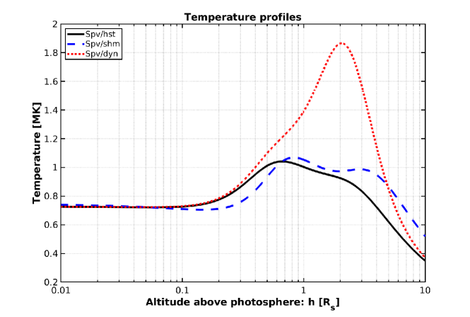
Figure 2.: The electron temperature profiles over the polar regions (Spv) calculated by using the three different methods: the scale height (SHM), the hydrostatic (HST), and the hydrodynamical (DYN). All three curves are calculated with the same polar electron density profile (Spv; the black-curve in figure 1) for which $\mathrm{n_{E}}$= 2.2 cm^-3 at 1 AU. The red dotted curve (Spv/DYN) is obtained by assuming that the SW velocity at 1 AU is equal to $\mathrm{u_{E}}$ = 329 km/s (which is an average value for slow SW flows), while the solid black-curve (Spv/HST) is obtained for $\mathrm{u_{E}}$ = 0; the DYN model coincides then with the hydrostatic HST model).F-temperature

The three electron temperatures profiles shown in figure F-temperature are obtained for the same polar density profile, Spv, by using the three different methods of calculation (SHM, HST, and DYN method) recalled above. This polar density profile is illustrated by the black curve in figure F-density. It corresponds to S70’s expended polar density distribution ( $\mathrm{\phi}=90\hbox{${}^{\circ}$}$) with $\mathrm{n_{E}}$ = 2.22 electrons/cc at 1 AU. A similar trio of temperature profiles were shown in figure 3 of Lemaire and Stegen (2016), obtained for the equatorial density distribution, Seq, corresponding to S70’s extended equatorial density distribution with $\mathrm{n_{E}}$ = 5.75 electrons/cm³ at 1 AU (i.e. the blue dashed curve in figure F-density).

In the DYN models shown in figure F-temperature and in all the following it is assumed that the temperature of the coronal protons is the same as that of the electrons ($\mathrm{T_{p}/T_{e}=\tau_{p}=1}$). Furthermore, it is assumed that the concentration of heavier ions is equal to zero ($\mathrm{n_{He^{++}}/n_{H^{+}}=\alpha=0}$). However, these questionable simplifications can easily be relaxed. In the current MATLAB® code developed by Lemaire and Stegen (2016), the value of $\alpha$ and $\mathrm{\tau_{p}}$ can be given different constant values which are independent of r. Results for such more evolved DYN models have been reported in Table 2 of Lemaire and Stegen (2016), and will not be repeated here.

Comparing both figures (figure F-temperature and figure 3 of Lemaire and Stegen, 2016) it can be seen that:

1. The maximum value of the SHM temperature distribution is always situated at a somewhat higher altitudes than the maximum value of the HST temperature. Indeed in the SHM method of calculation of $\mathrm{T_{e}(r)}$, the effect of the temperature gradient, $\mathrm{dT_{e}(r)/dr}$, is ignored (see Lemaire and Stegen, 2016), while it is properly taken into account in the HST method first developed by Alfvén (1941).

2. Both the SHM and the HST methods give maximum values, $\mathrm{T_{e,max}}$, that are nearly equal to each other (circa 1 MK, over the poles, and slight larger than 1.2 MK, over the equator).

3. the maximum of the DYN temperature is much larger than the maximum of the HST temperature over the poles (see figure F-temperature), while over the equatorial region, these two temperature maxima are almost identical (see figure 3 of Lemaire and Stegen (2016)); this is, of course, a consequence of the much larger coronal density over the equator.

4. The DYN and HST methods give almost identical temperatures profiles at low altitudes, for $\mathrm{h<0.1~{}R_{S}}$. This result is clearly foreseeable because at these lowest altitudes in the inner corona the coronal plasma is almost in hydrostatic equilibrium i.e. u(r) $\approx$ 0 both over the polar and equatorial regions.

5. In the inner corona the temperature gradients are positive : $\mathrm{dT_{e}(r)/dr}~{}>$ 0, but they tend to become smaller and smaller when r decreases to $\mathrm{r_{b}}$. This is a basic property satisfied both over the equator and the poles by all DYN solutions. This trend is, however, at odds with the temperature gradients predicted by the usual singular solutions of the hydrodynamical transport equations. Indeed in the latter critical hydrodynamical models the coronal temperature is in general a decreasing function of r, even at the base of the corona.

As a consequence of the much lower densities over the poles than over the equator, the radial distributions of the DYN and HST temperatures begin to depart from each other at much lower altitudes over the poles, than over the equatorial region. This occurs at h $\gtrapprox$ 0.2 $\mathrm{R_{S}}$ at high latitudes, while only at h $\gtrapprox$ 1 $\mathrm{R_{S}}$ (i.e. r $\gtrapprox$ 2 $\mathrm{R_{S}}$) over the lower equatorial latitudes.

any of the trends of the DYN temperatures outlined above and illustrated in figure F-temperature, as well as in figure 3 of Lemaire and Stegen (2016), are consistent with the observed properties of the solar corona temperatures reported in reviews, such as Echim, Lemaire, and Lie-Svendsen (2011).

The ongoing solar missions carry new kinds of instruments, such as the Wide-field Imager for Solar Probe (WISPR, Vourlidas et al., 2016) and Metis (Antonucci, Ester et al., 2019), capable of observing the $\mathrm{n_{e}(r)}$ distribution far more accurately and much more regularly than previously. The first results from WISPR are already published by Howard et al. (2019) and their figure 1 is in-line with S70’s density profiling. More results from those instruments are greatly anticipated by the authors as valuable input to the DYN models.

5 The effects of the input parameters $\mathrm{n_{E}}$ and $\mathrm{u_{E}}$ on the DYN temperature distribution

S-expansion

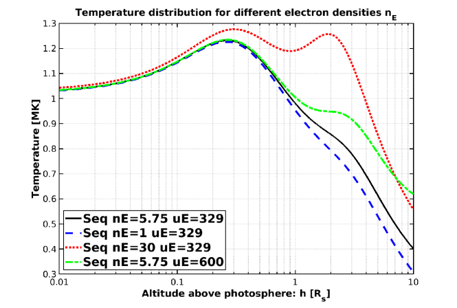
Figure 3.: Equatorial distributions of the DYN-temperature obtained for the following sets of the SW bulk velocity and electron density at 1 AU: $\mathrm{n_{E}}$= 1 $\mathrm{e^{-}/cm^{3}}$, $\mathrm{u_{E}}$ = 329 km/s (blue-dashed line); $\mathrm{n_{E}}$ =5.75 $\mathrm{e^{-}/cm^{3}}$, $\mathrm{u_{E}}$ = 329 km/s (black solid line); $\mathrm{n_{E}}$ = 30 $\mathrm{e^{-}/cm^{3}}$, $\mathrm{u_{E}}$ = 329 km/s (red dotted line); and $\mathrm{n_{E}}$ = 5.75 $\mathrm{e^{-}/cm^{3}}$, $\mathrm{u_{E}}$ = 600 km/s (dashed green line).F-nE

The figure 3 displays the DYN temperature profiles based on four different equatorial density profiles, $\mathrm{n_{e}(r,\phi)}$, corresponding to Saito’s extended density models for $\mathrm{\phi}=~{}90\hbox{${}^{\circ}$}$, $\mathrm{n_{E}}$ = 1.0; 5.75; 30.0 $\mathrm{e/cm^{3}}$, and $\mathrm{u_{E}}$ = 329; 600 km/s.

For the black curve in figure F-nE, $\mathrm{u_{E}}$ = 329 km/s and $\mathrm{n_{E}}$ = 5.75 $\mathrm{e/cm^{3}}$. These input parameters are respectively the SW bulk velocity and number density at 1 AU of the average slow SW flow (reported by Ebert et al., 2009). Two other curves (blue dashed and red dotted) show the DYN temperatures respectively for smaller and larger values of $\mathrm{n_{E}}$. It can be seen that when the solar wind density at 1 AU is reduced (from $\mathrm{n_{E}}$ = 5.75 to 1 $\mathrm{e/cm^{3}}$), the temperature profile is slightly reduced and tends to the HST temperature distribution. This can be see by comparing this curve to the Seq/HST curve in figure 3 of Lemaire and Stegen (2016); indeed, the latter was calculated by using the HST method introduced by Alfvén (1941). It comes as no surprise that the two are identical, since for a negligible amount of SW at 1 AU the DYN model becomes equivalent to the HST model.

However, when the SW density at 1AU is arbitrarily enhanced ($\mathrm{n_{E}}$ = 30 $\mathrm{e/cm^{3}}$ or more) it can be seen that a higher value of the maximum temperature is obtained in the mid-corona as expected to boost the coronal plasma to a bulk speed of $\mathrm{u_{E}}$ = 329 km/s or more, at 1 AU.

The green dotted curve in figure F-nE has a bump at h = 2 $\mathrm{R_{S}}$. This leads to the evidence that an enhanced maximum temperature, and thus an enhanced coronal heating rate, is required in the mid-corona in order to boost the SW speed at 1 AU up from 329 km/s (black curve corresponding to a slow SW flow) to 600 km/s (green curve; corresponding a fast wind speed).

The remarkable convergence at low altitudes of all four curves shown in figure F-nE tells us that the coronal temperature in the inner corona is almost unaffected by $\mathrm{n_{E}}$ and $\mathrm{u_{E}}$, the SW density and speed at 1 AU. It is basically the maximum DYN temperature within the mid-corona that determines the SW at 1 AU and in the distant interplanetary medium. In other words to enhance the SW expansion velocities or/and to enhance the plasma densities in the interplanetary medium, increased heating is not required at the base of the corona, but higher up in the corona at a radial distance of 3-4 $\mathrm{R_{S}}$. This is a most important new finding grounded on our DYN model calculations.

6 The differences between DYN models and Parker’s hydrodynamical models

S-boundary

The fundamental limitations of the hydrostatic coronal models are well understood. They were first pointed out in the papers by Parker (1958, 1963) The hydrodynamical plasma transport equations he introduced were integrated upwards from a low altitude reference level, $\mathrm{r_{0}}$, up to infinity. Very precisely chosen boundary condition, $\mathrm{u_{0}}$, had to be chosen at $\mathrm{r_{0}}$ to obtain a continuous solution for u(r) crossing a saddle point at the altitude where the SW expansion velocity becomes supersonic. Any other slightly different boundary conditions would produce diverging steady state solutions. In the 60’s this critical solution for the SW flow velocity had been compared to the similar hydrodynamical solution describing the supersonic flow velocity in a de Laval nozzle.

On the contrary, the DYN distributions of u(r) are continuous but non-singular solutions of the continuity and momentum equations describing the SW expansion. Indeed they are not characterized by a saddle point. In the DYN models these hydrodynamical transport equations are integrated downwards from 1 AU, where appropriate boundary conditions are taken as free input parameters. As indicated above this has the remarkable advantage to generate wide ranges of continuous solutions for the SW expansion velocity, and for the electron temperature distributions. Furthermore, all the latter DYN temperature profiles happen to converge at the base of the corona to HST temperature which corresponds to the hydrostatic model, whatever the values of $\mathrm{n_{E}}$ and $\mathrm{u_{E}}$, may have been assumed at 1 AU.

The singular solutions crossing a saddle point, lead to coronal temperatures that maximize at the base of the corona, having negative temperature gradients in the inner corona. But this is in contrast to the DYN temperature profiles which predict always that the values of $\mathrm{dT_{e}(r)/dr}$ are positive and small, both over the coronal poles (see figure F-temperature), and over the equator (see figure F-nE).

Note however, these nearly uniform values of $\mathrm{T_{e}(r)}$, in the inner corona, are larger in equatorial region (1.0-1.3 MK), than at high latitudes, over the poles and in coronal holes (0.7-0.8 MK). This remarkable difference of temperatures between the equatorial and polar in the inner corona, is well supported by SKYLAB and other EUV and X-ray observations.

Albeit in the inner corona ($\mathrm{h<0.1R_{S}}$) the nearly isothermal polar temperatures are much lower than the equatorial ones, the DYN models predict that the reverse is true at higher altitudes: i.e. in the mid-corona for h = 2-3 $\mathrm{R_{S}}$, when realistic values are adopted for $\mathrm{n_{E}}$ and $\mathrm{u_{E}}$.

From the results presented above, it can be seen that at such higher altitudes the maximum of the DYN temperatures is then much larger over the poles or in coronal holes ($\mathrm{T_{e,max}(r)}$ = 1.8-2.5 MK), than over the equatorial regions ($\mathrm{T_{e,max}(r)<1.3}$ MK). This result implies, thus, that much larger electron temperatures are indeed needed at mid-altitudes in coronal holes to accelerate SW streams to high speeds (600 km/s or more), than is needed over the equatorial regions from where the slower SW streams (330 km/s or so) are suspected to originate.

This conclusion is fully consistent with Parker’s expectation in the 60’s and Lemaire and Scherer (1971, 1973)’s one in the 70’s that larger coronal temperatures would necessarily be required in the corona, to boost the coronal plasma to larger speeds in interplanetary space. This leads us to infer that larger energy deposition rates are needed in the mid-corona, but not necessarily at lower altitudes inside the inner-corona.

Albeit in the present paper we do not address the pending issue of possible coronal heating mechanisms able to account for the DYN temperature profiles displayed in figures F-temperature and F-nE, we wish to insist that these profiles have their maximum in the mid-corona, not in the transition region at $\mathrm{h_{tr}\approx 0.003~{}R_{S}}$.

7 Conclusions

S-Conclusions

The calculated DYN temperature distributions have been compared with those determined by using older methods of calculation, especially, the SHM commonly used by assuming a corona in hydrostatic equilibrium and in isothermal equilibrium. It has been shown that the latter untenable assumptions are leading to coronal electron temperature distributions that are quite different from those obtained by the DYN method introduced by Lemaire and Stegen.

The DYN model is a straightforward extension of the hydrostatic model developed decades ago by Alfvén (1941). Indeed, it this more general model takes into account the radial expansion of the coronal plasma, without any transverse motion of plasma across magnetic field lines. Indeed, here it has been assumed that the coronal plasma is flowing up in open flow tubes that coincide with magnetic flux tubes whose geometry and cross-section, A(r), are the same as those adopted by Kopp and Holzer (1976). Here A(r) is an ad-hoc analytic input function associate to the DYN model.

The radial electron density distribution, $\mathrm{n_{e}(r)}$, is an additional input function required to create a DYN model. It can be derived from WL eclipse observations, or from an empirical model like that of Saito. Unfortunately, for A(r) there does not yet exist such a “steering oar” to guide our “educated guesses”.

After having pointed out the major differences between the temperature profiles obtained by the new DYN method in comparison to the SHM and HST models, we have shown that in all cases the calculated coronal temperatures have a maximum value in the mid-corona, and never at the base of the corona, as often implied in publications.

This important finding has lead us to the conjecture that the source of the coronal heating is not at the base of the corona, but higher up in the mid-corona, where the DYN temperatures distributions have a well defined maximum at all heliospheric latitudes. Note that even the HST temperature and SHM temperature profiles have temperature maxima well above the base of the corona.

These theoretical results put in question the common hypothesis that the corona is heated exclusively from below. Indeed, although widely spread, this believe is only a hypothesis based on the reasonable expectation that heating takes place where the energy density is at its highest. However, to the best of the authors knowledge, there are no evidence to rule out the possibility that a significant amount of heating takes place higher up.

Conversely, the DYN model cannot rule out the existence of the commonly-suggested heating mechanisms (such as those based on reconnection or magneto-hydrodynamical dumping). As it can be seen in figures F-temperature and F-nE and also in Lemaire and Stegen (2016), the temperature calculated at $\mathrm{r_{b}}$ is much higher than the observed chromospheric temperatures.

Obviously this cannot be considered as the end of the SW modelling venture but it is nevertheless a basic new step ahead. Much more elaborate and difficult work stays to model the kinetic pressure anisotropies of the electrons and ionic populations as well as their mutual collisional interactions, the most important and interesting challenge remaining, of course, the determination of the coronal heat deposition rate versus heliospheric distances and latitudes.

Acknowledgments

We acknowledge the logistic support of BELSPO, the Belgian Space Research Office, as well as the help of the IT teams of BIRA and ROB. JFL wishes also to thanks Viviane Pierrard (BIRA-IASB), Marius Echim (BIRA-IASB), Koen Stegen (ROB), and the early assistance of Clément Botquin, IT student hired during the Summer 2010. We acknowledge Serge Koutchmy for his interest in our work, and for pointing out in page 3664 of Lemaire and Stegen a mistake in the given numerical value of H (the density scale height at the base of the Corona when the temperature is assumed to be equal to 1 MK). ACK acknowledges funding from the Solar-Terrestrial Centre of Excellence (STCE), a collaborative framework funded by the Belgian Science Policy Office (BELSPO). Some work for this paper was also done in the framework of the SOL3CAM project (Contract: BR/154/PI/SOL3CAM), funded by BELSPO.

The authors are not aware of any conflicts of interest. The authors have no relevant financial or non-financial interests to disclose. All work done for this article was funded by the Royal Belgian Institute for Space Aeronomy (BIRA-IASB), and the Royal Observatory of Belgium (ROB). Both institutes are funded by the BELgian Science Policy Office (BELSPO).

References

- Alfvén (1941) Alfvén, H.: 1941, On the solar corona. Ark. Mat. Astron. Fys. 27, 1.
- Antonucci, Ester et al. (2019) Antonucci, Ester, Romoli, Marco, Andretta, Vincenzo, Fineschi, Silvano, Heinzel, Petr, Daniel Moses, J., et al.: 2019, Metis: the solar orbiter visible light and ultraviolet coronal imager. A&A. DOI. https://doi.org/10.1051/0004-6361/201935338.
- Baumbach (1937) Baumbach, S.: 1937, Strahlung, ergiebigkeit and electronendichte der sonnenkorona. Astron. Nachr. 263, 121.
- Ebert et al. (2009) Ebert, R.W., McComas, D.J., Elliott, H.A., Forsyth, R.J., Gosling, J.T.: 2009, Bulk properties of the slow and fast solar wind and interplanetary coronal mass ejections measured by Ulysses: Three polar orbits of observations. Journal of Geophysical Research (Space Physics) 114(A1), A01109. DOI. ADS.
- Echim, Lemaire, and Lie-Svendsen (2011) Echim, M.M., Lemaire, J., Lie-Svendsen, Ø.: 2011, A Review on Solar Wind Modeling: Kinetic and Fluid Aspects. Surveys in Geophysics 32(1), 1. DOI. ADS.
- Howard et al. (2019) Howard, R.A., Vourlidas, A., Bothmer, V., Colaninno, R.C., DeForest, C.E., Gallagher, B., Hall, J.R., Hess, P., Higginson, A.K., Korendyke, C.M., Kouloumvakos, A., Lamy, P.L., Liewer, P.C., Linker, J., Linton, M., Penteado, P., Plunkett, S.P., Poirier, N., Raouafi, N.E., Rich, N., Rochus, P., Rouillard, A.P., Socker, D.G., Stenborg, G., Thernisien, A.F., Viall, N.M.: 2019, Near-Sun observations of an F-corona decrease and K-corona fine structure. Nature 576, 232. DOI. ADS.
- Kopp and Holzer (1976) Kopp, R.A., Holzer, T.E.: 1976, Dynamics of coronal hole regions. I. Steady polytropic flows with multiple critical points. Sol. Phys. 49(1), 43. DOI. ADS.
- Lemaire and Scherer (1971) Lemaire, J., Scherer, M.: 1971, Kinetic models of the solar wind. J. Geophys. Res. 76(31), 7479. DOI. ADS.
- Lemaire and Scherer (1973) Lemaire, J., Scherer, M.: 1973, Kinetic models of the solar and polar winds. Reviews of Geophysics and Space Physics 11, 427. DOI. ADS.
- Lemaire and Stegen (2016) Lemaire, J.F., Stegen, K.: 2016, Improved Determination of the Location of the Temperature Maximum in the Corona. Sol. Phys. 291(12), 3659. DOI. ADS.
- Parker (1958) Parker, E.N.: 1958, Suprathermal Particles. III. Electrons. Physical Review 112(5), 1429. DOI. ADS.
- Parker (1963) Parker, E.N.: 1963, Interplanetary dynamical processes. ADS.
- Pottasch (1960) Pottasch, S.R.: 1960, Use of the Equation Hydrostatic Equilibrium in Determining the Temperature Distribution in the Outer Solar Atmosphere. ApJ 131, 68. DOI. ADS.
- Saito (1970) Saito, K.: 1970, A non-spherical axisymmetric model of the solar K corona of the minimum type. Annals of the Tokyo Astronomical Observatory 12(2), 53. ADS.
- Scarf and Noble (1965) Scarf, F.L., Noble, L.M.: 1965, Conductive Heating of the Solar Wind. II. The Inner Corona. ApJ 141, 1479. DOI. ADS.
- Vourlidas et al. (2016) Vourlidas, A., Howard, R.A., Plunkett, S.P., Korendyke, C.M., Thernisien, A.F.R., Wang, D., Rich, N., Carter, M.T., Chua, D.H., Socker, D.G., Linton, M.G., Morrill, J.S., Lynch, S., Thurn, A., Van Duyne, P., Hagood, R., Clifford, G., Grey, P.J., Velli, M., Liewer, P.C., Hall, J.R., DeJong, E.M., Mikic, Z., Rochus, P., Mazy, E., Bothmer, V., Rodmann, J.: 2016, The Wide-Field Imager for Solar Probe Plus (WISPR). Space Sci. Rev. 204(1-4), 83. DOI. ADS.