Modified Poisson-Nernst-Planck model with Coulomb and hard-sphere correlations

Abstract

We develop a modified Poisson-Nernst-Planck model which includes both the long-range Coulomb and short-range hard-sphere correlations in its free energy functional such that the model can accurately describe the ion transport in complex environment and under a nanoscale confinement. The Coulomb correlation including the dielectric polarization is treated by solving a generalized Debye-Hückel equation which is a Green’s function equation with the correlation energy of a test ion described by the self Green’s function. The hard-sphere correlation is modeled through the modified fundamental measure theory. The resulting model is available for problems beyond the mean-field theory such as problems with variable dielectric media, multivalent ions, and strong surface charge density. We solve the generalized Debye-Hückel equation by the Wentzel-Kramers-Brillouin approximation, and study the electrolytes between two parallel dielectric surfaces. In comparison to other modified models, the new model is shown more accurate in agreement with particle-based simulations and capturing the physical properties of ionic structures near interfaces.

1 Introduction

Ion transport in nanoscale systems is of essential importance in many physical phenomena and biological processes, and has attracting broad interest [1, 2]. The Poisson-Nernst-Planck (PNP) model is one of the most widely used models to describe the ion transport in fluids, where the dynamics of ions is composed of the diffusion and the convection, and the convection is due to the gradient of the electric potential governed by the Poisson’s equation. Analytical and numerical analysis based on the PNP model has been successfully applied to understand problems in areas such as nanofluidics, ion channels and semiconductor devices [3, 4, 5, 6].

The classical PNP model is a mean-field theory as the electrostatic energy in the Nernst-Planck (NP) equations is the mean potential energy. This model ignores ion-ion correlation, solvation energy due to variable dielectric permittivity, dielectric boundary effects and the excluded volume effects, and thus for many instances it cannot provide accurate description of particle interactions, significantly influencing the correct understanding of physical properties of electrolytes. For example, when divalent ions are present in the electrolyte, the ions cannot be treated as point charges without size effect, and with large surface charges the long-range Coulomb correlation cannot be ignored in order to capture many-body phenomena such as charge inversion and counterion condensation effects. Many efforts have been made on the improvement of the mean-field theory in literature [7, 8, 9, 10, 11, 12, 13] in order to make the model more physical. More recently, the contributions from different components such as ion-ion correlations and excluded volume effects are systematically studied in Ref. [14].

To take into account the long-range Coulomb correlation, Bazant et al. [15] proposed a phenomenological electrostatic free-energy functional treating ion-ion correlations by Landau-Ginzburg-type theory, and this work has been further developed in many studies [16, 17, 18, 19, 20]. Another promising approach to include the long-range correlation is to correct the mean potential by the self energy of ions under the idea of the Gaussian variational field theory [21, 22, 23] where the self energy of a test ion can be defined by the diagonal of a Green’s function described by the generalized Debye-Hückel (GDH) equation and the many-body physics due to the ionic correlation and dielectric image charges are both included [24, 25]. Beyond the point charge approximation, Wang [26] discussed the importance of the ionic self energy with finite size, developed a field-theoretical model with Gaussian charge distribution to represent the test ion, which can be simplified to the Born-energy augmented Poisson-Boltzmann theory by assuming the ionic radius being a small parameter for problems with variable dielectric permittivity. Liu et al. [27] assumes the test ion being a hard sphere with a point charge at the center and obtains the free energy functional by the Debye charging process using asymptotic expansion with the spherical radius as small parameter, which includes the Coulomb correlation of ions with finite size and the dielectric effect, such that the total self energy is described as the combination of the mean-field energy and correlation self energy where the Born solvation energy is the leading contribution for variable media. This type of modified PNP models satisfies the energy dissipation law and a proper weak formulation, and has been successfully applied in exploring important physical properties, such as like-charge attraction and double layer structure [28, 29]. As an alternative approach, the density functional theory has also been extensively studied in the past few decades where long-range Coulomb correlation by integral equation theory such as hypernetted-chain and mean spherical approximations [30, 31, 32, 33].

Another key factor for the ion transport is the steric effect of ions. Though the finite size is included in the model of Coulomb correlation, the short-range non-electrostatic correlation is not accounted for. For simple systems of hard-sphere (HS) fluids, short-range interactions are generally repulsive arising from the excluded volume effect of particles, more precisely, the Pauli exclusion that prevents two electrons from occupying the same quantum state. Among various models for implementing the HS interactions, the density functional theory has been widely utilized as a powerful approach by capturing the non-local contributions to the free energy functional, where the fundamental measure theory (FMT) proposed by Rosenfeld [34] has been shown to investigate the HS systems successfully. There are many subsequent work to make the improvements of the FMT from different aspects. It is widely accepted now that the steric interaction for the HS model can be accurately calculated by the modified fundamental measure theory (MFMT) [35, 36] for the excess free energy functional. In the FMT, the excess Helmholtz energy functional can be expressed as a weighted density approximation which can provide a more accurate description of properties of inhomogeneous HS fluids and becomes the same as that from the scaled particle theory [37] or the Percus-Yevick theory [38] in the limit of homogeneous hard spheres. The original FMT overestimates the contact value of density distribution and shows evident deviations under strong confinements in comparison to Monte Carlo simulations. Yu and Wu [36] and Roth et al. [35] proposed the MFMT by using a more accurate Helmholtz energy density from the Boublik-Mansoori-Carnahan-Starling-Leland equation of state for the HS correlation. Further, Jiang et al. [39] generalized it to transport problems and obtained the time-dependent density functional theory using the framework of the NP equations. Separately, there are also many other theories describing the excess free energy of steric effects such as those based on the Lennard-Jones kernel[40, 41, 10], entropic effect of solvent molecules [42, 43, 44, 45, 11], and Carnahan Starling local density[46].

Besides contributions to the continuum theory, there have been plenty of results based on particle-based simulations for primitive electrolytes and they are in general thought as benchmarks to different theoretical models due to proper treatments of Coulombic correlations and steric effects. For instance, the planar system without dielectric mismatches is well discussed by a recent systematic Monte Carlo (MC) study [47] and references therein. For problems with dielectric interfaces that is related to current work, we refer to MC studies [48, 49, 50, 51, 52] and recent molecular dynamic (MD) simulations [53].

In this work, we propose a new modified PNP model for the ion transport, which contains both the long-range Coulomb and the short-range HS correlations. In the model, the total energy of an ion in the system consists of three contributions, the mean-field electrostatic energy by the Poisson’s equation, the Coulomb self energy by the GDH equation and the excess Helmholtz energy from the MFMT. The Wentzel-Kramers-Brillouin (WKB) approach is proposed for problems with two parallel dielectric interfaces and the contribution of the Stern layer is accounted for in this approach, which is essential to the accuracy of the approximation. By the WKB approximation, the modified PNP model can be efficiently solved by finite-difference numerical methods. Comparisons among classical mean-field PNP, and different versions of modified PNP equations are made, together with particle-based simulations. Our numerical simulations demonstrate that the new model can accurately predict the oscillation of the ionic density as well as depletion zone near highly charged dielectric interfaces. Furthermore, the combined effects of dielectric boundary and ionic size in current model are well presented and discussed through simulations with various parameter groups.

The rest of the paper is organized as follows. In Sec. 2, we formulate the modified PNP model with including long- and short-range correlations through an energetic approach. In Sec. 3, a two-plate model together with its dimensionless form is described and the method for solving the modified PNP system is proposed. In Sec. 4, numerical calculations are performed to show the attractive feature of the model. The conclusion remarks are finally made in Sec. 5.

2 Modified Poisson-Nernst-Planck model

We consider the ionic dynamics in electrolytes composed of $K$ ionic species. Let $c_{i}(\bm{r};t)$ be the ionic density of the $i$-th species at time $t$ and $z_{i}$ be its valence. The evolution of the ionic densities obeys the general conservation law,

$$\frac{\partial c_{i}}{\partial t}=-\nabla\cdot\bm{J}_{i},$$ (1)

where the ionic flux can be described by the constitutive relation with the electrochemical potential $\bar{\mu}_{i}$,

$$\bm{J}_{i}=-b_{i}c_{i}\nabla\bar{\mu}_{i},$$ (2)

with $b_{i}$ being the ionic mobility of the $i$-th species. With the ionic density given, the distribution of electric potential $\phi$ over the space is governed by the Poisson’s equation,

$$-\nabla\cdot\varepsilon\nabla\phi=\rho_{f}+\sum_{i=1}^{K}z_{i}ec_{i},$$ (3)

where $\varepsilon$ is the dielectric permittivity of the medium, $\rho_{f}$ is the fixed charge density in space, and $e$ is the elementary charge. The dielectric permittivity is a physical quantity that could depend on position, electric field or ionic concentrations [54, 55, 56, 57, 58, 59, 60], and this work assumes a space-dependent function $\varepsilon(\bm{r})$.

To connect the electrochemical potential with the electric potential and ionic densities, we consider an energetic approach by a variation of the total free energy $F$ with respect to the ionic density, that leads to $\bar{\mu}_{i}=\delta F/\delta c_{i}$. We assume that the charged system in domain $\Omega$ is composed of ions represented by charged hard-spheres. In this work, the total free energy is decomposed into three contributions, expressed by the following formula,

$$F=F^{\textup{mf}}+F^{\textup{co}}+F^{\textup{hs}},$$ (4)

where $F^{\textup{mf}}$ is the electrostatic free energy of mean-field approximation, $F^{\textup{co}}$ is the Coulomb correlation energy, and $F^{\textup{hs}}$ describes the excess free energy due to HS repulsive interactions.

The free energy is a functional of the ionic density vector $\bm{c}=(c_{1},\cdots,c_{K})$. The mean-field electrostatic free energy has been widely studied and is given by,

$$\begin{split}F^{\textup{mf}}[\bm{c}]=\int_{\Omega}\left[\frac{\varepsilon(\bm{r})}{2}|\nabla\phi(\bm{r})|^{2}+k_{B}T\sum_{i=1}^{K}c_{i}\left(\ln\Lambda^{3}c_{i}-1\right)\right]d\bm{r},\end{split}$$ (5)

where the potential is the solution of the Poisson’s equation together with some boundary conditions, $k_{B}$ is the Boltzmann constant, $T$ is the absolute temperature and $\Lambda$ is the thermal de Broglie wavelength. The chemical potential due to this functional is,

$$\mu_{i}^{\textup{mf}}=\frac{\delta F^{\textup{mf}}}{\delta c_{i}}=z_{i}e\phi+k_{B}T\ln c_{i}.$$ (6)

When $\bar{\mu}_{i}$ is replaced by this chemical potential, one obtains the classical NP equations from Eq. (1), and thus the PNP equations coupled with the Poisson’s equation (3). At equilibrium, the density minimizes the free energy, that gives straightforwardly a constant chemical potential. This results in the classical Boltzmann distribution to represent the ionic density as function of $\phi$, and leads to the mean-field Poisson-Boltzmann equation,

$$-\nabla\cdot\varepsilon\nabla\phi=\rho_{f}+\sum_{i=1}^{K}z_{i}ec_{i}^{\textup{b}}\exp{\left(-\beta z_{i}e\phi\right)},$$ (7)

where $\beta=1/(k_{B}T)$ and $c_{i}^{\textup{b}}$ is the bulk-state ion density.

As discussed in the Introduction, the PNP and Poisson-Boltzmann models are mean-field theories and cannot capture many-body effects, and to go beyond correlations should be taken into account. The excess free energies due to long-range Coulomb and short-range HS correlations, $F^{\textup{co}}$ and $F^{\textup{hs}}$ as functionals of the ionic densities will be discussed separately below, which result in the corresponding components for chemical potentials, $\mu_{i}^{\textup{co}}=\delta F^{\textup{co}}/\delta c_{i}$ and $\mu_{i}^{\textup{hs}}=\delta F^{\textup{hs}}/\delta c_{i}$. The total electrochemical potential is $\bar{\mu}_{i}=\mu_{i}^{\textup{mf}}+\mu_{i}^{\textup{co}}+\mu_{i}^{\textup{hs}}$. Finally, by Eqs. (1) and (2), one obtains the modified NP equations,

$$\frac{\partial c_{i}}{\partial t}=\nabla\cdot\left[D_{i}\nabla c_{i}+b_{i}c_{i}\nabla\left(z_{i}e\phi+\mu_{i}^{\textup{co}}+\mu_{i}^{\textup{hs}}\right)\right],\quad i=1,...,K,$$ (8)

where $D_{i}$ is the ion diffusivity connecting the ionic mobility by the Einstein relation $D_{i}=k_{B}Tb_{i}$. Alternatively, one can denote by $U_{i}=z_{i}e\phi+\mu_{i}^{\textup{co}}+\mu_{i}^{\textup{hs}}$ the potential of mean force that means the energy cost to move a single ion from bulk to the current position. Together with the Poisson’s equation (3), the coupled system is named as the modified PNP equations and is self-consistent because $\mu_{i}^{\textup{co}}$ and $\mu_{i}^{\textup{hs}}$ are functions depending on ion densities only, as shown in Sec. 2.1 and 2.2.

2.1 Coulomb correlation

The long-range Coulomb correlation is the long-range electrostatic correlation, including both the ion-ion correlation beyond mean field and the dielectric self energy of ions [27]. By the Debye charging process, the Coulomb correlation can be written as,

$$F^{\textup{co}}=\int d\bm{r}\int_{0}^{1}d\lambda^{2}\sum_{i=1}^{K}c_{i}(\bm{r})\left[U^{\textup{Born}}_{i}(\bm{r})+U_{i}^{\lambda}(\bm{r})\right],$$ (9)

where $\lambda\in[0,1]$ is increased from 0 to 1, that represents the charging process, and $U^{\textup{Born}}_{i}(\bm{r})$ is the Born solvation energy [61] which is space-dependent for an inhomogeneous dielectric medium. The second term in the bracket of Eq. (9) is the $\lambda$-dependent part due to the Coulomb correlation, which by the point charge approximation is given by,

$$U_{i}^{\lambda}(\bm{r})=\frac{1}{2}\sum_{j=1}^{K}\int_{\Omega}c_{j}(\bm{r}^{\prime})h_{ij}^{\lambda}(\bm{r},\bm{r}^{\prime})v_{ij}(\bm{r},\bm{r}^{\prime})d\bm{r}^{\prime},$$ (10)

where

$$v_{ij}(\bm{r},\bm{r}^{\prime})=z_{i}z_{j}e^{2}G_{0}(\bm{r},\bm{r}^{\prime}),$$ (11)

is the pairwise potential contribution arising from the electrostatic interaction, with the Green’s function $G_{0}$ satisfying

$$-\nabla\cdot\varepsilon(\bm{r})\nabla G_{0}(\bm{r},\bm{r}^{\prime})=\delta(\bm{r}-\bm{r}^{\prime}),$$ (12)

and $h_{ij}^{\lambda}(\bm{r},\bm{r}^{\prime})$ is the $\lambda$-dependent pair correlation function.

The remaining step is to obtain the pair correlation function $h^{\lambda}_{ij}$ that can be determined by the Ornstein-Zernike equation [62],

$$h^{\lambda}_{ij}(\bm{r},\bm{r}^{\prime})=c^{\lambda}_{ij}(\bm{r},\bm{r}^{\prime})+\int\sum_{k=1}^{K}c_{k}(\bm{r}^{\prime\prime})h^{\lambda}_{jk}(\bm{r}^{\prime},\bm{r}^{\prime\prime})c^{\lambda}_{ik}(\bm{r},\bm{r}^{\prime\prime})d\bm{r}^{\prime\prime}.$$ (13)

In order to close the system, one applies the random phase approximation for the direct correlation function $c^{\lambda}_{ij}$, i.e., $c^{\lambda}_{ij}=-\beta\lambda^{2}v_{ij}$ [63]. Similarly to the expression of Eq. (11), one can write

$$h^{\lambda}_{ij}(\bm{r},\bm{r}^{\prime})=-\beta z_{i}z_{j}e^{2}h_{\lambda}(\bm{r},\bm{r}^{\prime}).$$ (14)

Together with Eq. (11), one substitutes the expressions of $h^{\lambda}_{ij}$ and $c^{\lambda}_{ij}$ into the Ornstein-Zernike equation, and obtains,

$$-h_{\lambda}(\bm{r},\bm{r}^{\prime})=\lambda^{2}\int G_{0}(\bm{r},\bm{r}^{\prime\prime})\left[2I(\bm{r}^{\prime\prime})h_{\lambda}(\bm{r}^{\prime},\bm{r}^{\prime\prime})-\delta\left(\bm{r}^{\prime}-\bm{r}^{\prime\prime}\right)\right]d\bm{r}^{\prime\prime},$$ (15)

with the ionic strength expressed by

$$I(\bm{r})=\frac{1}{2}\beta e^{2}\sum_{i=1}^{K}z_{i}^{2}c_{i}(\bm{r}).$$

Thus, one can write the $\lambda$-dependent part of the correlation energy as

$$U_{i}^{\lambda}(\bm{r}) =-z_{i}^{2}e^{2}\int G_{0}(\bm{r},\bm{r}^{\prime})I(\bm{r}^{\prime})h_{\lambda}(\bm{r},\bm{r}^{\prime})d\bm{r}^{\prime}$$ (16)

$$=\frac{1}{2}z_{i}^{2}e^{2}\lim_{\bm{r}^{\prime}\rightarrow\bm{r}}\left[\frac{h_{\lambda}(\bm{r},\bm{r}^{\prime})}{\lambda^{2}}-G_{0}(\bm{r},\bm{r}^{\prime})\right]$$

$$=\frac{1}{2}z_{i}^{2}e^{2}\lim_{\bm{r}^{\prime}\rightarrow\bm{r}}\left[G_{\lambda}(\bm{r},\bm{r}^{\prime})-G_{0}(\bm{r},\bm{r}^{\prime})\right]$$

where one has denoted by the $\lambda$-dependent Green’s function $G_{\lambda}=h_{\lambda}/\lambda^{2}$ that can be determined by the differential equation transformed from Eq. (15), i.e., the generalized Debye-Hückel equation,

$$-\nabla\cdot\varepsilon(\bm{r})\nabla G_{\lambda}(\bm{r},\bm{r}^{\prime})+2\lambda^{2}I(\bm{r})G_{\lambda}(\bm{r},\bm{r}^{\prime})=\delta(\bm{r}-\bm{r}^{\prime}).$$ (17)

The excess chemical potential coming from the Coulomb correlation is now derived as

$$\mu_{i}^{\textup{co}}(\bm{r})=\frac{\delta F^{\textup{co}}}{\delta c_{i}}=U_{i}^{\textup{Born}}(\bm{r})+\frac{\delta}{\delta c_{i}}\int d\bm{r}\int_{0}^{1}d\lambda^{2}\sum_{j=1}^{K}c_{j}(\bm{r})U_{j}^{\lambda}(\bm{r}).$$ (18)

The integration with respect to $\lambda$ can be performed analytically. For the purpose, we use Eqs. (15) and (16) to expand $U_{j}^{\lambda}(\bm{r})$ as,

$$U_{j}^{\lambda}(\bm{r})=\frac{z_{j}^{2}e^{2}}{2}\sum_{k=1}^{\infty}(-1)^{k}\lambda^{2k}\beta_{k}(\bm{r}),$$ (19)

with $\beta_{k}$ the integral of form

$$\beta_{k}(\bm{r})=\int d\bm{r}_{1}\cdots\int d\bm{r}_{k}\left[G_{0}(\bm{r},\bm{r}_{1})2I(\bm{r}_{1})\cdots G_{0}(\bm{r}_{k-1},\bm{r}_{k})2I(\bm{r}_{k})G_{0}(\bm{r}_{k},\bm{r})\right].$$

Thus, with Eq. (19) plugged in, the last term in Eq. (18) can be reformulated into

$$\frac{1}{\beta}\int_{0}^{1}d\lambda\frac{\delta}{\delta c_{i}}\int d\bm{r}\left[2I(\bm{r})\sum_{k=1}^{\infty}(-1)^{k}\lambda^{2k+1}\beta_{k}(\bm{r})\right]$$

$$= \frac{z_{i}^{2}e^{2}}{2}\int_{0}^{1}d\lambda\sum_{k=1}^{\infty}2(k+1)(-1)^{k}\lambda^{2k+1}\beta_{k}(\bm{r})$$

$$= \int_{0}^{1}d\lambda\frac{d\left(\lambda^{2}U_{i}^{\lambda}(\bm{r})\right)}{d\lambda}$$

$$= U_{i}^{\lambda=1}(\bm{r}),$$ (20)

where we have utilized the property,

$$\frac{\delta}{\delta c_{i}}\left(\int 2I(\bm{r})\beta_{k}(\bm{r})d\bm{r}\right)=\beta z_{i}^{2}e^{2}(k+1)\beta_{k}(\bm{r}).$$

Clearly, we have that the free energy contribution is exactly the correlation energy at the full charging.

For the ease of asymptotic analysis, the chemical potential is further rearranged as

$$\mu_{i}^{\textup{co}}(\bm{r})= U_{i}^{\textup{Born}}(\bm{r})+U_{i}^{\lambda=1}(\bm{r})$$

$$= \left[U_{i}^{\textup{Born}}(\bm{r})+\frac{1}{2}z_{i}^{2}e^{2}\lim_{\bm{r}^{\prime}\rightarrow\bm{r}}\left(\frac{1}{4\pi\varepsilon(\bm{r})|\bm{r}-\bm{r}^{\prime}|}-G_{0}(\bm{r},\bm{r}^{\prime})\right)\right]$$

$$\quad\quad+\frac{1}{2}z_{i}^{2}e^{2}\lim_{\bm{r}^{\prime}\rightarrow\bm{r}}\left[G_{\lambda=1}(\bm{r},\bm{r}^{\prime})-\frac{1}{4\pi\varepsilon(\bm{r})|\bm{r}-\bm{r}^{\prime}|}\right].$$ (21)

We now apply the strategies of asymptotic expansions from Ref. [27] (Sec. 2.3.2) to the part within the first bracket in Eq. (21) and have its leading order term, i.e., the $O(1/a_{i})$ term, as the following Born solvation energy,

$$\frac{z_{i}^{2}e^{2}}{8\pi a_{i}}\left(\frac{1}{\varepsilon(\bm{r})}-\frac{1}{\varepsilon_{0}}\right),$$ (22)

with $a_{i}$ the radius of the $i$th ion. It should be noted that using ion radius in (22) is an approximation and could lead to a poor prediction sometimes as compared to experiments because the ion and Born radii differ and produce very different Born energies for real electrolytes. The point charge assumption involved in Eq. (10) has generated the decoupling of the size effect embodied in Born energy (22) and the ion-ion interactions related to $G_{\lambda}$ as described by Eq. (17). For more general cases of size-dependent $G_{\lambda}$ and higher-order correction to the Born energy, we refer systematical analysis to the asymptotic work in Ref. [27].

It is noted that there is another way used to obtain the chemical potential, called the Güntelberg charging process [64] where only the central charge of the test ion is increased from zero to the full charging and other ions remain full charges during the process. It was shown [27] that the Debye and Güntelberg charging processes are equivalent in the case of the point charge approximation. It is then straightforward to have the following expression for the Coulomb correlation component of the chemical potential,

$$\mu^{\textup{co}}_{i}=\frac{z_{i}^{2}e^{2}}{2}\left[\frac{1}{4\pi a_{i}}\left(\frac{1}{\varepsilon(\bm{r})}-\frac{1}{\varepsilon_{0}}\right)+\lim_{\bm{r}^{\prime}\rightarrow\bm{r}}\left(G(\bm{r},\bm{r}^{\prime})-\frac{1}{4\pi\varepsilon(\bm{r})|\bm{r}-\bm{r}^{\prime}|}\right)\right],$$ (23)

where $G(\bm{r},\bm{r}^{\prime})=G_{\lambda=1}(\bm{r},\bm{r}^{\prime})$ is the Green’s function satisfying the GDH equation with full charging,

$$-\nabla\cdot\varepsilon(\bm{r})\nabla G(\bm{r},\bm{r}^{\prime})+2I(\bm{r})G(\bm{r},\bm{r}^{\prime})=\delta(\bm{r}-\bm{r}^{\prime}).$$ (24)

It is mentioned that from now on we have omitted $t$ in notations for time-dependent ionic densities and related variables, for instance, $c_{i}(\bm{r})=c_{i}(\bm{r};t)$ and $G(\bm{r},\bm{r}^{\prime})=G(\bm{r},\bm{r}^{\prime};t)$. In order to involve the boundary effects, one needs to define the ionic strength profile in general as

$$I(\bm{r}) =\left\{\begin{array}[]{ll}\frac{1}{2}\beta e^{2}\sum_{i=1}^{K}z_{i}^{2}c_{i}(\bm{r}),~{}~{}\bm{r}\in\Omega,\\ 0,~{}~{}~{}~{}~{}~{}~{}~{}~{}~{}~{}~{}~{}~{}~{}~{}~{}~{}~{}~{}~{}~{}~{}~{}\bm{r}\notin\Omega,\end{array}\right.$$ (27)

and consider the inhomogeneous dielectric permittivity profile. Noteworthily, the GDH equation (24) has been applied to the exterior of the electrolyte besides taking into account the ion-ion interactions within the electrolyte, that means the dielectric property and absence of ions in the boundary domain, or equivalently, the dielectric boundary effects are effectively implemented in our model.

2.2 Hard-sphere correlation

In addition to long-range Coulomb correlations, there are also non-electrostatic HS interactions that are generally repulsive and short-ranged. Various models have been developed for the HS interactions such as FMT [34] and its modifications [35, 36]. This work uses the MFMT which accurately approximates the excess Helmholtz energy density and has been shown promising to provide an efficient implementation of HS interactions [35, 36, 65, 66]. Since the MFMT has been discussed in many literatures, here we present the basic idea of the theory.

In the MFMT, the excess Helmholtz free energy due to HS interactions can be expressed by a weighted density approximation,

$$F^{\textup{hs}}[\bm{c}]=k_{B}T\int f^{\textup{hs}}[\bm{c}(\bm{r})]d\bm{r},$$ (28)

where the excess Helmholtz energy density $f^{\textup{hs}}$ is written as a function of six weighted densities which are functionals of the ionic densities, including four scalar densities $n_{\alpha}(\bm{r}),(\alpha=0,\cdots,3),$ and two vector densities $\bm{n}_{a}(\bm{r})$ and $\bm{n}_{b}(\bm{r})$, precisely,

$$f^{\textup{hs}}[\bm{c}(\bm{r})]= -n_{0}\ln(1-n_{3})+\frac{n_{1}n_{2}-\bm{n}_{a}\bm{n}_{b}}{1-n_{3}}$$

$$+\frac{(1-n_{3})^{2}\ln(1-n_{3})+n_{3}}{36\pi n_{3}^{2}(1-n_{3})^{2}}\left(n_{2}^{3}-3n_{2}\bm{n}_{b}\cdot\bm{n}_{b}\right).$$ (29)

The weighted densities are defined by the weighted averages of ionic densities,

$$n_{\alpha}(\bm{r})=\sum_{i=1}^{K}n^{(\alpha)}_{i}(\bm{r})=\sum_{i=1}^{K}\int c_{i}(\bm{r}^{\prime})\omega_{i}^{(\alpha)}(\bm{r}-\bm{r}^{\prime})d\bm{r}^{\prime},$$ (30)

where the relevant six weight functions are classified into four scalar weights,

$$\omega_{i}^{(0)}(\bm{r}) =\frac{\omega_{i}^{(1)}(\bm{r})}{a_{i}}=\frac{\omega_{i}^{(2)}(\bm{r})}{4\pi a_{i}^{2}}=\frac{\delta(a_{i}-r)}{4\pi a_{i}^{2}},\quad\omega_{i}^{(3)}(\bm{r})=\theta(a_{i}-r),$$ (31)

and the two vector-type weights,

$$\bm{\omega}_{i}^{a}(\bm{r})=\frac{\bm{\omega}_{i}^{b}(\bm{r})}{4\pi a_{i}}=\frac{\bm{r}}{r}\frac{\delta(a_{i}-r)}{4\pi a_{i}}.$$ (32)

Here $r=|\bm{r}|$, $\delta(\cdot)$ and $\theta(\cdot)$ are the Dirac delta and the Heaviside step functions, respectively. It can be seen that $\omega_{i}^{(1)}$ and $\omega_{i}^{(2)}$ are proportional to $\omega_{i}^{(0)}$, $\bm{\omega}_{i}^{b}$ is proportional to $\bm{\omega}_{i}^{a}$, and thus there are actually only two scalar weights and one vector weight. Eventually, $F^{\textup{hs}}$ turns out to be a functional of ion densities only. As a consequence, the variational derivative of excess free energy with respect to the ionic density leads to the corresponding HS excess chemical potential, where the derivatives of energy density to weighted densities can be obtained from Eq. (29) straightforwardly.

3 Two-plate problem

In this section, one considers the solution of a two-plate problem with an electrolyte placed in between two parallel electrodes by solving the modified PNP model. This problem is often used in the understanding of the ionic structure near interfaces, and is of importance in many electrochemical devices such as charge storages and water purification.

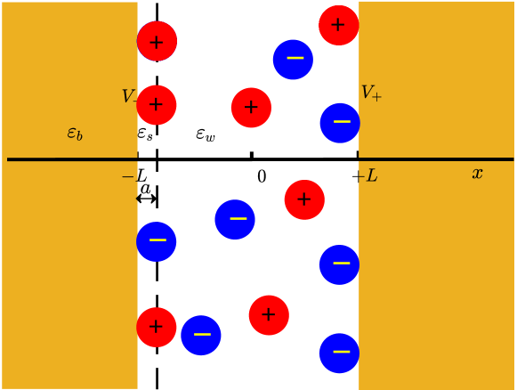
Fig. 1: Schematic representation of a two-plate problem. Ions are inaccessible to the Stern layers of thickness $a$. Separation of two interfaces is $2L$ and dielectric coefficient is piecewise-constant with $\varepsilon_{s}$ in the Stern layers, different from the ion-accessible region and the electrode region.

3.1 Dimensionless equations

We assume that two interfaces are located at $x=\pm L$ with voltages $V_{\pm}$ (as shown in Fig. 1). The electrolyte region near each electrode surface is divided into an ion-impenetrable Stern layer with thickness $a=\min_{i}{a_{i}}$ and a diffuse layer of mobile ions. Note that the dielectric profile within the electrolyte could be generally inhomogeneous, for instance, space-dependent near surfaces, concentration- or electric field-dependent. However, to simplify the model setup, the inhomogeneous dielectric profile of the entire domain is assumed to be homogeneous along $yz$ directions, and is described by the piecewise function $\varepsilon(x)$ which is $\varepsilon_{s}$ in the Stern layers $L-a\leq|x|\leq L$, $\varepsilon_{w}$ in the ion-accessible region $|x|<L-a$, and $\varepsilon_{b}$ in the electrode region $|x|>L$. The modified PNP equations for the ion-accessible region are given by,

$$-\varepsilon_{w}\frac{\partial^{2}\phi}{\partial x^{2}}=\sum_{i}z_{i}ec_{i},$$ (33)

$$\frac{\partial c_{i}}{\partial t}=\frac{\partial}{\partial x}\left[D_{i}\frac{\partial}{\partial x}c_{i}+b_{i}c_{i}\frac{\partial}{\partial x}\left(z_{i}e\phi+\mu^{\textup{co}}_{i}+\mu^{\textup{hs}}_{i}\right)\right].$$ (34)

The weighted densities associated with the HS correlation are simplified as one dimensional integrals,

$$n_{i}^{(0)}(x)=\frac{1}{2a_{i}}\int_{x-a_{i}}^{x+a_{i}}c_{i}(x^{\prime})dx^{\prime},$$ (35)

$$n_{i}^{(3)}(x)=\pi\int_{x-a_{i}}^{x+a_{i}}c_{i}(x^{\prime})[a_{i}^{2}-(x^{\prime}-x)^{2}]dx^{\prime},$$ (36)

$${\bm{n}}_{i}^{a}(x)=\frac{\bm{e}_{x}}{2a_{i}}\int_{x-a_{i}}^{x+a_{i}}c_{i}(x^{\prime})(x^{\prime}-x)dx^{\prime},$$ (37)

and $n_{i}^{(1)},n_{i}^{(2)}$ and $\bm{n}_{i}^{b}$ are defined consequently.

Simultaneously, the GDH equation associated with $\mu^{\textup{co}}_{i}$ is reduced to

$$-\nabla\cdot\varepsilon(x)\nabla G+2I(x)G=\delta(\bm{r}-\bm{r}^{\prime}).$$ (38)

Note that the Green’s function is three-dimensional with the geometrical symmetry although the dielectric and ionic strength profiles are simply one-dimensional, i.e., $G=G(x,x^{\prime},\rho)$ with $\rho=\sqrt{(y-y^{\prime})^{2}+(z-z^{\prime})^{2}}$. Below we focus on the asymptotic treatment of its approximation for the solution of the GDH equation.

At interfaces between the Stern and diffuse layers $x=\pm(L-a)$, proper boundary conditions have to be applied to solve modified PNP. Precisely, the Laplace equation for $\phi$ within the Stern layer gives the Robin boundary conditions,

$$\phi\pm a\frac{\varepsilon_{w}}{\varepsilon_{s}}\frac{\partial\phi}{\partial x}=V_{\pm}.$$ (39)

Additionally, we consider the no surface-reactions assumption that leads to the no-flux boundary conditions,

$$\bm{J}_{i}\cdot\bm{n}=D_{i}\left(\frac{\partial c_{i}}{\partial x}+\beta c_{i}\frac{\partial U_{i}}{\partial x}\right)=0.$$ (40)

Finally, the far-field boundary condition for Green’s function reads $\lim_{\bm{r}\rightarrow\infty}G(\bm{r},\bm{r}^{\prime})=0.$ These boundary conditions together with the initial data of the ionic concentrations uniquely determine the solution of the modified PNP system.

As a further step, the quantities in the system are nondimensionalized by using $\varepsilon_{w}$ for dielectric permittivity, the bulk density $c_{0}$ for ion densities, $1/(\beta e)$ for potentials, $L$ for length, the uniform $D_{0}(=D_{i})$ for diffusivities, $L\ell_{0}/D_{0}$ for time with the length scale defined by $\ell_{0}=1/\sqrt{8\pi\ell_{\textup{B}}c_{0}}$ which is the Debye length for a 1:1 electrolyte and the Bjerrum length $\ell_{\textup{B}}=\beta e^{2}/(4\pi\varepsilon_{w})$.

For electrostatic-related variables, $G$ and $\mu_{i}^{\textup{co}}$ are rescaled by $1/(\beta e^{2})$ and $1/\beta$, respectively, that gives the dimensionless chemical potential,

$$\mu_{i}^{\textup{co}}=\frac{1}{2}z_{i}^{2}\left[\frac{q}{a_{i}}\left(\frac{1}{\eta(x)}-\frac{1}{\eta_{0}}\right)+\lim_{\bm{r}^{\prime}\rightarrow\bm{r}}\left(G(\bm{r},\bm{r}^{\prime})-\frac{q}{\eta(x)|\bm{r}-\bm{r}^{\prime}|}\right)\right],$$ (41)

where $\eta$ is the rescaled dielectric profile, the dimensionless parameter is $q=\ell_{\textup{B}}/L$, and $G$ satisfies the dimensionless GDH equation,

$$-\nabla\cdot\eta(x)\nabla G+\frac{I(x)}{\epsilon^{2}}G=4\pi q\delta(\bm{r}-\bm{r}^{\prime}).$$ (42)

Here comes the second dimensionless parameter $\epsilon=\ell_{0}/L$, and the spatial dependent dielectric and ionic strength profiles are

$$\eta(x)=\left\{\begin{array}[]{ll}1,\quad|x|<1-a,\\ \eta_{s},\quad 1-a\leq|x|\leq 1,\\ \eta_{b},\quad|x|>1.\end{array}\right.\quad I(x)=\left\{\begin{array}[]{ll}\sum_{i}z_{i}^{2}c_{i}(x)/2,\quad|x|<1-a,\\ 0,\quad\quad\quad\quad\quad\quad|x|\geq 1-a.\end{array}\right.$$ (43)

At the HS side, $\mu_{i}^{\textup{hs}}$ is rescaled by $1/\beta$ and the weighted densities $n_{\alpha}$ are rescaled by $\nu=c_{0}L^{3}=1/(8\pi q\epsilon^{2})$. Consequently, the dimensionless integrals transformed from the variation of Eq. (28) can be evaluated directly though detailed formulae are omitted here.

Finally, we obtain the dimensionless form of the modified PNP,

$$-2\epsilon^{2}\frac{\partial^{2}}{\partial x^{2}}\phi=\sum_{i=1}^{K}z_{i}c_{i},\quad|x|\leq 1-a,$$ (44)

$$\frac{\partial c_{i}}{\partial t}=\epsilon\frac{\partial}{\partial x}\left[\frac{\partial}{\partial x}c_{i}+c_{i}\frac{\partial}{\partial x}\left(z_{i}\phi+\mu^{\textup{co}}_{i}+\mu^{\textup{hs}}_{i}\right)\right],\quad|x|\leq 1-a,$$ (45)

with boundary conditions

$$\phi\pm a\frac{1}{\eta_{s}}\frac{\partial\phi}{\partial x}=V_{\pm},\quad x=\pm(1-a),$$ (46)

$$\frac{\partial c_{i}}{\partial x}+c_{i}\frac{\partial}{\partial x}(z_{i}\phi+\mu^{\textup{co}}_{i}+\mu^{\textup{hs}}_{i})=0,\quad x=\pm(1-a).$$ (47)

As an important quantity in investigating electric double layers, the total diffuse charge near one electrode is also considered. The dimensionless value of that, without loss of generality, near the negative-charged electrode is

$$Q(t)=\int_{-1+a}^{0}\sum_{i=1}^{K}z_{i}c_{i}(x,t)dx.$$ (48)

3.2 WKB approximation

The Green’s function involved in the GDH equation is generally six-dimensional and dependent on both $\bm{r}$ and $\bm{r}^{\prime}$. Due to the symmetry in the geometry, the system can be simplified by Fourier transform and reduced to a two-dimensional equation that can be solved efficiently by selected inversion method [67]. Nevertheless, in this paper we extend the WKB asymptotic approach to propose an approximate model that can be solved analytically to give the final solution. The dimensionless parameter that represents the dielectric mismatch is clearly visualized in the form of the asymptotic solution and shall provide more intuitive insights for physical understandings.

The WKB approximation for the GDH equation was first introduced by Buff and Stillinger [68] for one-plate problem. The WKB method solves the Green’s function problem for a salt-free system by the image-charge theory, and then approximates the salty system by using screened Coulomb potential to replace each Coulomb potential where the inverse screening parameter is given by the average between $x$ and $x^{\prime}$, i.e.,

$$\kappa^{\prime}(x,x^{\prime})=\frac{1}{x-x^{\prime}}\int_{x^{\prime}}^{x}\kappa(s)ds.$$

This method was later extended to solve two-plate problem [24]. For the system we are studying, the three-layer structure in each electrode results in a difficulty for an image theory. To derive the WKB approximation, one starts from the following original Debye-Hückel equation of constant coefficient,

$$-\nabla^{2}\widetilde{G}+{\kappa}^{2}\widetilde{G}=4\pi q\delta(\bm{r}-\bm{r}^{\prime}),$$ (49)

for $|x|<1-a$, and $-\nabla^{2}\widetilde{G}=0$ otherwise, where $\kappa$ is the inverse Debye length which is a constant approximating $\sqrt{I}/\epsilon$.

Though our treatment is believed to be useful for a more general dielectric profile, we focus on the effect of $\eta_{b}$ and consider a uniform dielectric permittivity in the electrolyte, i.e., one sets $\eta_{s}=1$ to avoid tedious derivation. Thus, the Born energy in Eq. (41) is constant and can be normalized, and one can write the general solution of $\widetilde{G}$ with far-field boundary conditions in terms of the following integrals,

$$\frac{\widetilde{G}}{q}=\begin{cases}\begin{array}[]{l}\int_{0}^{\infty}{C_{l}(\omega,x^{\prime})e^{\omega x}}J_{0}(\rho\omega)d\omega,\quad x<-1,\\ \int_{0}^{\infty}{\left[D_{l}(\omega,x^{\prime})e^{\omega x}+E_{l}(\omega,x^{\prime})e^{-\omega x}\right]}J_{0}(\rho\omega)d\omega,\quad-1<x<-1+a,\\ \int_{0}^{\infty}\frac{e^{-\tau(\omega)|x-x^{\prime}|}+A(\omega,x^{\prime})e^{\tau(\omega)x}+B(\omega,x^{\prime})e^{-\tau(\omega)x}}{\tau(\omega)}J_{0}(\rho\omega)\omega d\omega,\quad|x|<1-a,\\ \int_{0}^{\infty}{\left[D_{r}(\omega,x^{\prime})e^{\omega x}+E_{r}(\omega,x^{\prime})e^{-\omega x}\right]}J_{0}(\rho\omega)d\omega,\quad 1-a<x<1,\\ \int_{0}^{\infty}{C_{r}(\omega,x^{\prime})e^{-\omega x}}J_{0}(\rho\omega)d\omega,\quad x>1,\end{array}\end{cases}$$ (50)

where $J_{0}$ is the Bessel function, $\tau(\omega)=\sqrt{\omega^{2}+{\kappa}^{2}}$ and $\rho=\sqrt{(y-y^{\prime})^{2}+(z-z^{\prime})^{2}}$. The coefficients $A$, $B$, $C_{l}$, $C_{r}$, $D_{l}$, $D_{r}$, $E_{l}$ and $E_{r}$ are solved with continuities of electric potentials and displacements on $x=\pm(1-a)$ and $x=\pm 1$. Specifically, for the domain of interest, i.e., $|x|<1-a$, we have

$$A(\omega,x^{\prime}) =\frac{-e^{\tau x^{\prime}}+f_{1}(\omega)e^{-\tau(x^{\prime}+2-2a)}}{e^{2\tau(1-a)}/f_{1}(\omega)-f_{1}(\omega)e^{-2\tau(1-a)}},$$ (51)

$$B(\omega,x^{\prime}) =\frac{-e^{-\tau x^{\prime}}+f_{1}(\omega)e^{\tau(x^{\prime}-2+2a)}}{e^{2\tau(1-a)}/f_{1}(\omega)-f_{1}(\omega)e^{-2\tau(1-a)}},$$ (52)

where the dielectric boundary effect has been embedded into $f_{1}$ through the dimensionless parameter $\gamma=(1-\eta_{b})/(1+\eta_{b})$, i.e.,

$$f_{1}(\omega)=\frac{\omega-\tau{\left(e^{2\omega a}+\gamma\right)}/{\left(e^{2\omega a}-\gamma\right)}}{\omega+\tau{\left(e^{2\omega a}+\gamma\right)}/{\left(e^{2\omega a}-\gamma\right)}}.$$

Consistently, the referenced free-space Green’s function is rewritten into the integral form,

$$\frac{1}{|\bm{r}-\bm{r}^{\prime}|}=\int_{0}^{\infty}e^{-\omega|x-x^{\prime}|}J_{0}(\rho\omega)d\omega,$$ (53)

and then we obtain the difference in the limit that is further defined as the rescaled electrostatic correlation energy $u_{\textup{el}}$, i.e.,

$$u_{\textup{el}}= \lim_{\bm{r}^{\prime}\rightarrow\bm{r}}\left({\widetilde{G}}/{q}-{1}/{|\bm{r}-\bm{r}^{\prime}|}\right)$$

$$= \lim_{\rho\rightarrow 0,\ x^{\prime}\rightarrow x}\left[\widetilde{G}(x,x^{\prime},\rho)-\int_{0}^{\infty}e^{-\omega|x-x^{\prime}|}J_{0}(\rho\omega)d\omega\right]$$

$$= \lim_{x^{\prime}\rightarrow x}\int_{0}^{\infty}\left(\frac{\omega e^{-\tau|x-x^{\prime}|}}{\tau}-e^{-\omega|x-x^{\prime}|}\right)d\omega+\int_{0}^{\infty}\frac{2f_{1}e^{-2\tau(1-a)}-e^{2\tau x}-e^{-2\tau x}}{e^{2\tau(1-a)}/f_{1}-f_{1}e^{-2\tau(1-a)}}\frac{\omega}{\tau}d\omega$$

$$= -\kappa\left[1-\int_{1}^{\infty}\frac{2f_{2}e^{-2\kappa(1-a)t}-e^{2\kappa xt}-e^{-2\kappa xt}}{e^{2\kappa(1-a)t}/f_{2}-f_{2}e^{-2\kappa(1-a)t}}dt\right],$$ (54)

where $f_{2}(t)=f_{1}\left(\kappa\sqrt{t^{2}-1}\right)$.

The WKB approximation for a variable screening is simply to replace the constant $\kappa$ in Eq. (54) by function $\kappa(x)$. This treatment is asymptotically correct at both low and high screening limits. Obviously, the WKB approximation has considered the effects of the local ionic strength, the Stern layer and the dielectric boundary that are dominating unless the variation of ionic strength is quite significant. Thus, the WKB can generally produce well accuracy in solving the GDH, as demonstrated in Fig. 3 in Sec. 4. It is remarked that Ref. [24] studied the WKB approximation for two-plate problems where the Stern layer effect is not taken into account, and the new WKB is supposed to provide a better approximation.

3.3 Numerical method for the modified PNP system

Though many asymptotic works have been done for the PNP or modified systems [69, 70, 9, 71], the HS interactions in current model cause great challenges in any asymptotic analysis. Instead, we introduce full numerical methods for the nonlinear coupled equation system. As stated above, the excess chemical potentials $\mu^{\textup{co}}_{i}$ and $\mu^{\textup{hs}}_{i}$ are functions of $c_{i}$ only thus can be evaluated by independent numerical scheme at each time step. The main PNP system is then solved by proper schemes and serves to produce updated ion densities $c_{i}$ and electrostatic potential $\phi$.

For simplicity, we consider the binary electrolyte with symmetric size in this work, i.e, $a_{1}=a_{2}=a$ though our numerical schemes can be extended for general asymmetrical electrolytes. On the similar basis, we consider the boundary potentials as $V_{+}=-V_{-}=V$. The main PNP equations are solved numerically on the domain $|x|<1-a$. We introduce uniform half grid points $x_{n+1/2}=(-1+a)+nh$, $n=0,\cdots,N$, with spatial grid size $h=2(1-a)/N$ such that $x_{N+1/2}=1-a.$ Also, we define the integer grid points $x_{n}$ as the average of two neighboring half grid points with two additional ghost points $x_{0}=x_{1}-h$ and $x_{N+1}=x_{N}+h$. The uniform time steps are defined by, $t_{m}=(m-1)k,\ m=1,2,...$, with $k$ the uniform time step size.

For given ionic densities $c_{i}^{n,m}$ at time $t=t_{m}$ and position $x_{n}$, the electric potential is solved approximately by the discretization of the Poisson’s equation through a second-order central difference scheme,

$$-2\epsilon^{2}\frac{\phi^{n+1,m}-2\phi^{n,m}+\phi^{n-1,m}}{h^{2}}=\sum_{i}z_{i}c_{i}^{n,m},$$ (55)

with Robin boundary conditions on $x=\pm(1-a)$ approximated by,

$$\left(\frac{1}{2}+\frac{a}{h}\right)\phi^{0,m}+\left(\frac{1}{2}-\frac{a}{h}\right)\phi^{1,m} =V_{-},$$ (56)

$$\left(\frac{1}{2}-\frac{a}{h}\right)\phi^{N,m}+\left(\frac{1}{2}+\frac{a}{h}\right)\phi^{N+1,m} =V_{+}.$$ (57)

At next time step $t=t_{m+1}$, the ionic density is updated by the discretization of the modified NP equation

$$\partial_{t}c_{i}=\epsilon\partial_{x}\left(e^{-U_{i}}\partial_{x}g_{i}\right),$$ (58)

where the generalized Slotboom variables $g_{i}=c_{i}e^{U_{i}}$ is utilized with recalling that $U_{i}=z_{i}\phi+\mu^{\textup{co}}_{i}+\mu^{\textup{hs}}_{i}$. Following the strategies in [27, 72], we discretize the modified NP equation as follows,

$$\frac{c_{i}^{n,m+1}-c_{i}^{n,m}}{k}= \frac{\epsilon}{h}\left(e^{-U_{i}^{n+1/2,m+1/2}}\frac{g^{n+1,m+1/2}_{i}-g^{n,m+1/2}_{i}}{h}\right.$$

$$\left.-e^{-U_{i}^{n-1/2,m+1/2}}\frac{g^{n,m+1/2}_{i}-g^{n-1,m+1/2}_{i}}{h}\right),$$ (59)

with $g^{n,m+1/2}_{i}=c^{n,m+1/2}_{i}e^{-U^{n,m+1/2}_{i}},$ where proper approximations of averaging are given by

$$c^{n,m+1/2}_{i} =\frac{c_{i}^{n,m+1}+c_{i}^{n,m}}{2},$$ (60)

$$U^{n,m+1/2}_{i} =\frac{3U_{i}^{n,m}-U_{i}^{n,m-1}}{2},$$ (61)

$$U^{n+1/2,m}_{i} =\frac{U_{i}^{n+1,m}+U_{i}^{n,m}}{2}.$$ (62)

The no-flux boundary conditions lead to

$$\frac{g^{1,m+1/2}_{i}-g^{0,m+1/2}_{i}}{h}=\frac{g^{N+1,m+1/2}_{i}-g^{N,m+1/2}_{i}}{h}=0.$$ (63)

Note that the averages in Eqs. (61) and (62) have made all nonlinear terms including $\mu^{\textup{co}}_{i}$ and $\mu^{\textup{hs}}_{i}$ evaluated explicitly, and the implicit scheme from Eq. (60) leads to a final linear system that can be solved directly. This scheme has second order of accuracy and is stable under the condition $k={O}(h)$. Simultaneously, it is not difficult to prove that the mass conservation is satisfied automatically with time evolution.

4 Numerical results and discussion

In this section, we first validate the numerical schemes and then demonstrate the correctness of our theoretical model by comparing to particle-based simulation results. To validate the accuracy in computing HS interactions, uniform ionic densities $c_{i}(x)\equiv 1$ are used for the evaluation of excess HS chemical potentials with different $N$. Remaining parameters take $(\epsilon,q,a)=(0.2,0.3,0.15)$. The results are displayed in Fig. 2. We observe the convergence with the increase of $N$ in panel (a), and that the second order of accuracy is shown in panel (b) as expected for the linear interpolation utilized in the evaluation of integrals. Note that in panel (b) the errors are differences between numerical results and analytical solutions of $\mu^{\textup{hs}}(x=0)$.

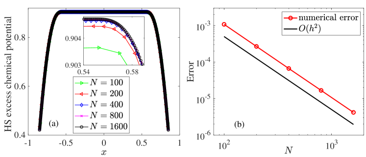
Fig. 2: Numerical convergence of computing the HS interactions: (a) chemical potential for different $N$; (b) Errors vs. $N$. Uniform ion density profiles $c_{i}(x)\equiv 1$ are assumed.

To show the accuracy of the proposed WKB approximation, the comparison of solutions of the modified PNP equations is presented in Fig. 3 where both the direct finite difference method (FDM) [67, 24] and the WKB are used in solving the GDH. The dimensionless dielectric constant of the plates is set to be $\eta_{b}=0.05$ where the repulsive effect on ion densities is expected. Other parameters chosen for this example are $(\epsilon,q,a,V)=(0.1,0.15,0.075,1)$, $z_{1}=-z_{2}=1$, $N=800$ and $k/h=1/2$. The density profiles are generally in good agreements except a slight deviation in a longer time simulation ($t=5$ in panel (b)) and both methods can capture the repulsive effect near the surface.

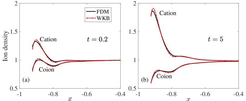
Fig. 3: Ionic density profiles from the solution of the modified PNP equations with a comparison between FDM and WKB for solving the GDH equation.

We next calculate the ion densities from the modified PNP model in comparison to the particle-based MC or MD simulations. We also calculate results from three different models for comparison, including the classical mean-field PNP, the modified PNP with only short-range HS correlation, the modified PNP with long-range Coulomb correlation, and the modified PNP proposed in current work with both long- and short-range correlations. For short, they are called MF, SC, LC and LS, respectively. As only equilibrium state is needed here, we take the Boltzmann distribution for ion densities expressed as $c_{i}=\exp(z_{i}\phi+\mu_{i}^{\textup{co}}+\mu_{i}^{\textup{hs}})$ and the resulting modified PB equation system is discretized by the FDM and solved iteratively [67, 25]. We start from the cases without dielectric mismatch on surfaces, i.e., $\gamma=0$, and the results are presented in Fig. 4 (a) where the MC simulation results are adopted from recent work [47]. For uncharged surfaces, the LS, LC and MC results predict the slight repulsion of ions near the surface due to the ionic depletion effect beyond the MF theory. Additionally, the agreement of MC and theoretical results (LS, LC) for the case with weakly charged surfaces ($0.02\ C/m^{2}$) is observed. Due to the weak HS correlation effect here, there is a very slight difference between the LS and LC models and the weak attraction near the uncharged surfaces is observed from SC model, which are similar to those in panels (b) and (c). In Fig. 4 (b), the cases of one single dielectric surface with high and low dielectric constants are studied. Our theoretical predictions from the LS and LC match the MC results [48, 49] well except a slight deviation approaching the dielectric-repulsive surface. In Fig. 4 (c), we calculate the system with two uncharged but dielectric surfaces. For both dielectric-repulsive and attractive surfaces, the LS and LC results agree well with MD simulations from the recent work[53]. We further study the case with significant HS correlation effects in panel (d) with uncharged surfaces, where the dimensionless parameters are $(\epsilon,q,a,\gamma)=(0.2,0.3,0.15,0.95)$ and the MD simulation is performed with the method in Ref. [53]. Large deviations from results of the four different models are depicted. The SC model predicts strong adsorption of ions near the surface due to the HS correlation, namely, particle repulsion in the interior region is stronger than those near the surface. In contrast, the LC model only predicts a rapid decline of ion density caused by the dielectric repulsion. As both long and short effects are competitive, the LS model produces the peak of density near the surface, which agrees well with the MD simulation. Note that there is an increased deviation approaching to the surface. This is due to the Lennard-Jones treatment in MD, instead of the hard spheres in the LS model. The detailed information for all corresponding dimensional parameters can be found in figure caption.

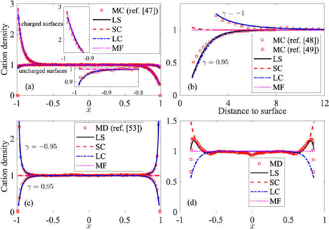
Fig. 4: Cation density profiles for $1:1$ electrolyte. (a) Two parallel surfaces without dielectric mismatch. MC results are from the free database of [47]. The dimensional parameters are $c_{0}=100$ mM, $a_{\pm}=0.15$ nm, $L=11.825$ nm. For the charged case, the surface charge densities are $\mp 0.02\ C/m^{2}$ on the left and right surfaces. The insets show profiles more clearly near the surfaces. (b) One single uncharged dielectric surface with the distance to the surface in the unit of the ion radius $a_{\pm}=0.15$ nm. MC results of the $\gamma=-1$ case are from [49] (solid squares in their figure 3) with $c_{0}=50$ mM, and those of the $\gamma=0.95$ case are from [48] (in their figure 4 (c)) with $c_{0}=500$ mM. (c) Two dielectric surfaces. MD results are from [53] (in their figure 5 left) where $c_{0}=90$ mM, $L=5$ nm and $a_{\pm}=0.1$ nm. (d) Two dielectric surfaces with parameters $\gamma=0.95$, $c_{0}=424$ mM, $L=2.33$ nm and $a_{\pm}=0.35$ nm and simulation results are obtained by MD [53]. The Bjerrum length $\ell_{\textup{B}}$ is $0.714$ nm in (ab) and $0.7$ nm in (cd).

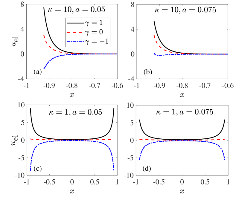
Fig. 5: The rescaled electrostatic correlation energy (defined in Eq. (54)) with different dielectric ratios and a homogeneous ionic strength.

In the rest of the paper, three cases of parameter $\gamma=1,0,-1$ are considered. Our WKB results show that the dielectric effect is enhanced with the decrease of $\kappa a$ which corresponds to a more dilute electrolyte and/or smaller ionic size (thinner Stern layer thickness). As a simple case to validate the model, we assume the artificial environment with homogeneous ionic strength, $\kappa(x)\equiv\kappa$, and test the rescaled electrostatic correlation energy $u_{\textup{el}}$ (54) with $\kappa=10,1$ and $a=0.05,0.075$, where effects of dielectric boundaries are well visualized in Fig. 5.

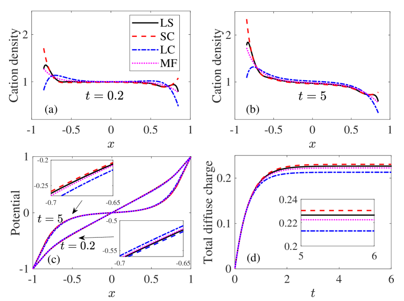
Fig. 6: Cation density, potential and total diffuse charge profiles for four different models.

We next simulate the modified PNP system by studying the 1:1 binary electrolyte with fixing $V=1$ and varying the dimensionless parameters $(\epsilon,q,a,\gamma)$. Fig. 6 shows the results with parameters $(\epsilon,q,a,\gamma)=(0.2,0.3,0.15,1)$. The cation densities are shown in panels (a) and (b) at time $t=0.2$ and $t=5$, where the overlapping of electric double layers on both interfaces has been observed due to the relatively large value of $\epsilon$. Compared with MF, the SC model enhances the density profile obviously while the LC model causes the repulsive effect because of the high dielectric ratio $\gamma=1$ which means the low dielectric permittivity of the boundary materials. The density profile from the LS model is close to that from the SC model away from the surface, but the deviation is increased as approaching the Stern layer due to the repulsive effect. Both the depletion and the layering effects are observed in the LS model in agreement with the physical intuition of the double-layer structure, demonstrating the importance of including both the long-range and short-range correlations in the modified PNP theory.

Fig. 6 (c, d) displays potential and total diffuse charge profiles from the four different models. The total diffuse charges present a clear discrepancy in the four models when the system tends to the steady state at long time. This is due to the opposite effects between the Coulomb correlation and HS correlation, where the former decreases the diffuse charge and the latter improves it. Therefore, the model with only the long-range correlation underestimates the total diffuse charge, and that with only the HS correlation overestimates it.

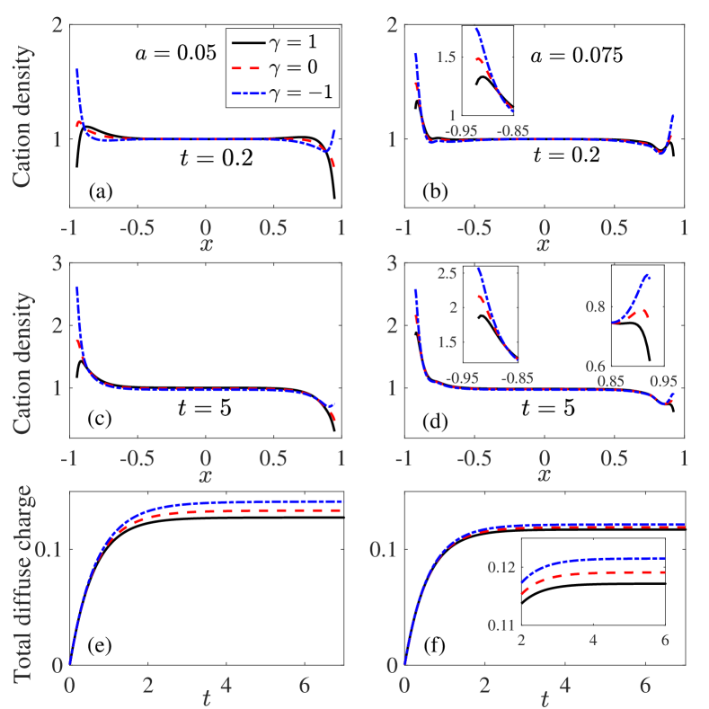
Fig. 7: Cation density, potential and diffuse charge profiles with different dielectric ratios for ionic size (ace) $a=0.05$ and (bdf) $a=0.075$.

To have a closer look at mutual effects of dielectric boundaries and HS interactions, we study the solutions of the LS model by varying $\gamma$ and $a$ with fixed $(\epsilon,q,V)$. In Fig. 7, we present the cation density and diffuse charge for $a=0.05$ and $0.075$ and different $\gamma$ values. The deviations for different $\gamma$ are larger for a smaller size $a$ (a, c) because of the reduced effect of HS interactions in comparison to the dielectric effect and the thinner Stern layer thickness enhancing the dielectric boundary effect. When $a$ increases (b, d), the density oscillating behavior starts to occur and the deviations in density profiles with different $\gamma$ are reduced. From panels (e, f), the attractive effect in the case of high electrode permittivity ($\gamma=-1$) enhances the total diffuse charge. Similarly, the deviations in diffuse charges decrease for larger $a$ due to the reduced dielectric effect.

5 Conclusion

By taking into account both long-range Coulomb and short-range HS correlations through an energetic approach, we have made proper improvements to the classical PNP model and developed a self-consistent modified PNP model including both correlations. The Coulomb correlation energy is obtained by solving the GDH equation, and the HS interaction is captured accurately by the MFMT. We have demonstrated the significant improvements of our modified PNP by comparing it with mean-field or other partially modified models through the two-plate problem with a piecewise-constant dielectric profile. An accurate and efficient hybrid numerical method, which incorporates the WKB approximation for GDH into a stable and mass-conservative scheme for the main PNP, has been developed to solve the entire two-plate modified PNP model. By calculating the results for systems with different values of $\gamma$ and $a$, we have explored the competitive effects from the dielectric ratio and ionic size, which is essentially the main motivation of the current work.

The present modified PNP model serves as a powerful approach beyond the mean-field treatment considering that both long- and short-range correlations play the same important role in many practical systems at the micro/nano scale. As one of the possible applications, the phenomena of the like-charge attraction or charge inversion is worth to be explored by the current model. The competition between the surface charge and the dielectric repulsive effect has been considered to lead to like-charge attraction or charge inversion [73]. Recently, a general theory is developed to consider the effects of strong ion-ion correlations and short-range hydration interactions on surface forces [19]. A systematic study with surface charge, long-range electrostatic correlation (including dielectric boundary effect) and short-range HS interaction on these many-body phenomena will be of much interest and will be the goal of future work.

References

- [1] R. B. Schoch, J. Han, and P. Renaud, Transport phenomena in nanofluidics, Rev. Mod. Phys., 80 (2008), pp. 839–883.
- [2] R. H. French, V. A. Parsegian, R. Podgornik, R. F. Rajter, A. Jagota, J. Luo, D. Asthagiri, M. K. Chaudhury, Y.-m. Chiang, S. Granick, S. Kalinin, M. Kardar, R. Kjellander, D. C. Langreth, J. Lewis, S. Lustig, D. Wesolowski, J. S. Wettlaufer, W.-Y. Ching, M. Finnis, F. Houlihan, O. A. von Lilienfeld, C. J. van Oss, and T. Zemb, Long range interactions in nanoscale science, Rev. Mod. Phys., 82 (2010), pp. 1887–1944.
- [3] M. Z. Bazant, K. Thornton, and A. Ajdari, Diffuse-charge dynamics in electrochemical systems, Phys. Rev. E, 70 (2004), p. 021506.
- [4] P. Markowich, C. Ringhofer, and C. Schimeiser, Semiconductor, Springer, New York, 1990.
- [5] B. Eisenberg, Crowded charges in ion channels, Adv. Chem. Phys., 148 (2012), pp. 77–223.
- [6] B. Eisenberg and W. Liu, Poisson-Nernst-Planck systems for ion channels with permanent charges, SIAM J. Math. Anal., 38 (2007), pp. 1932–1966.
- [7] A. B. Mamonov, R. D. Coalson, A. Nitzan, and M. G. Kurnikova, The role of the dielectric barrier in narrow biological channels: A novel composite approach to modeling single-channel currents, Biophys. J., 84 (2003), pp. 3346–3661.
- [8] B. Corry, S. Kuyucak, and S.-H. Chung, Dielectric self-energy in Poisson-Boltzmann and Poisson-Nernst-Planck models of ion channels, Biophys. J., 84 (2003), pp. 3594–3606.
- [9] M. S. Kilic, M. Z. Bazant, and A. Ajdari, Steric effects in the dynamics of electrolytes at large applied voltages. II. Modified Poisson–Nernst–Planck equations, Phys. Rev. E, 75 (2007), p. 021503.
- [10] B. Eisenberg, Y. Hyou, and C. Liu, Energy variational analysis of ions in water and channels: Field theory for primitive models of complex ionic fluids, J. Chem. Phys., 133 (2010), p. 104104.
- [11] B. Lu and Y. C. Zhou, Poisson-Nernst-Planck equations for simulating biomolecular diffusion-reaction processes II: Size effects on ionic distributions and diffusion-reaction rates, Biophys. J., 100 (2011), pp. 2475–2485.
- [12] S. Ji and W. Liu, Poisson-Nernst-Planck systems for ion flow with density functional theory for hard-sphere potential: I-V relations and critical potentials. Part I: Analysis, J. Dyn. Diff. Equ., 24 (2012), pp. 955–983.
- [13] D. Frydel, Mean-field electrostatics beyond the point-charge description, Adv. Chem. Phys., 160 (2016), pp. 209–260.
- [14] A. Voukadinova and D. Gillespie, Energetics of counterion adsorption in the electrical double layer, J. Chem. Phys., 150 (2019), p. 154706.
- [15] M. Z. Bazant, B. D. Storey, and A. A. Kornyshev, Double layer in ionic liquids: Overscreening versus crowding, Phys. Rev. Lett., 106 (2011), p. 046102.
- [16] B. D. Storey and M. Z. Bazant, Effects of electrostatic correlations on electrokinetic phenomena, Phys. Rev. E, 86 (2012), p. 056303.
- [17] J.-L. Liu and B. Eisenberg, Correlated ions in a calcium channel model: A Poisson-Fermi theory, J. Phys. Chem. B, 117 (2013), pp. 12051–12058.
- [18] B. Ciotti and B. Li, Legendre transforms of electrostatic free-energy functionals, SIAM J. Appl. Math, 78 (2018), pp. 2973–2995.
- [19] R. P. Misra, J. P. de Souza, D. Blankschtein, and M. Z. Bazant, Theory of surface forces in multivalent electrolytes, Langmuir, 35 (2019), pp. 11550–11565.
- [20] J. P. de Souza and M. Z. Bazant, Continuum theory of electrostatic correlations at charged surfaces, J. Phys. Chem. C, 124 (2020), pp. 11414–11421.
- [21] R. Podgornik, Electrostatic correlation forces between surfaces with surface specific ionic interactions, J. Chem. Phys., 91 (1989), pp. 5840–5849.
- [22] R. R. Netz and H. Orland, Beyond Poisson-Boltzmann: Fluctuation effects and correlation functions, Eur. Phys. J. E, 1 (2000), pp. 203–214.
- [23] R. R. Netz and H. Orland, Variational charge renormalization in charged systems, Eur. Phys. J. E, 11 (2003), pp. 301–311.
- [24] Z. Xu, M. Ma, and P. Liu, Self-energy-modified Poisson-Nernst-Planck equations: WKB approximation and finite-difference approaches, Phys. Rev. E, 90 (2014), p. 013307.
- [25] M. Ma and Z. Xu, Self-consistent field model for strong electrostatic correlations and inhomogeneous dielectric media, J. Chem. Phys., 141 (2014), p. 244903.
- [26] Z.-G. Wang, Fluctuation in electrolyte solutions: The self energy, Phys. Rev. E, 81 (2010), p. 021501.
- [27] P. Liu, X. Ji, and Z. Xu, Modified Poisson-Nernst-Planck model with accurate Coulomb correlation in variable media, SIAM J. Appl. Math., 78 (2018), pp. 226–245.
- [28] P. Liu, M. Ma, and Z. Xu, Understanding depletion induced like-charge attraction from self-consistent field model, Comm. Comp. Phys., 22 (2017), pp. 95–111.
- [29] L. Ji, P. Liu, Z. Xu, and S. Zhou, Asymptotic analysis on dielectric boundary effects of modified Poisson-Nernst-Planck equations, SIAM J. Appl. Math., 78 (2018), pp. 1802–1822.
- [30] E. Kierlik and M. Rosinberg, Density-functional theory for inhomogeneous fluids: adsorption of binary mixtures, Phys. Rev. A, 44 (1991), p. 5025.
- [31] Y. Rosenfeld, Free energy model for inhomogeneous fluid mixtures: Yukawa-charged hard spheres, general interactions, and plasmas, J. Chem. Phys., 98 (1993), pp. 8126–8148.
- [32] D. Gillespie, W. Nonner, and R. S. Eisenberg, Density functional theory of charged, hard-sphere fluids, Phys. Rev. E, 68 (2003), p. 031503.
- [33] R. Roth and D. Gillespie, Shells of charge: a density functional theory for charged hard spheres, J. Phys.: Condens. Matter, 28 (2016), p. 244006.
- [34] Y. Rosenfeld, Free energy model for the inhomogeneous hard-sphere fluid mixture and density-functional theory of freezing, Phys. Rev. Lett., 63 (1989), p. 011301.
- [35] R. Roth, R. Evans, A. Lang, and G. Kahl, Fundamental measure theory for hard-sphere mixtures revisited: the white bear version, J. Phys.: Condens. Matter, 14 (2002), p. 12063.
- [36] Y.-X. Yu and J. Wu, Structures of hard-sphere fluids from a modified fundamental-measure theory, J. Chem. Phys., 117 (2002), pp. 10156–10164.
- [37] H. Riess, H. L. Frisch, and J. L. Lebowitz, Statistical mechanics of rigid spheres, J. Chem. Phys., 31 (1959), pp. 369–380.
- [38] J. L. Lebowitz and J. S. Rowlison, Thermodynamic properties of mixtures of hard sphere, J. Chem. Phys., 41 (1964).
- [39] J. Jiang, D. Cao, D.-e. Jiang, and J. Wu, Time-dependent density functional theory for ion diffusion in electrochemical systems, J. Phys.: Condens. Matter, 26 (2014), p. 284102.
- [40] F.-H. Lin, C. Liu, and P. Zhang, On hydrodynamics of viscoelastic fluids, Commun. Pure Appl. Math., 58 (2005), pp. 1437–1471.
- [41] P. Sheng, J. Zhang, and C. Liu, Onsager principle and electrorheological fluid dynamics, Prog. Theor. Phys. Suppl., 175 (2008), pp. 131–143.
- [42] I. Borukhov, D. Andelman, and H. Orland, Steric effects in electrolytes: A modified Poisson-Boltzmann equation, Phys. Rev. Lett., 79 (1997), pp. 435–438.
- [43] B. Li, Continuum electrostatics for ionic solutions with non-uniform ionic sizes, Nonlinearity, 22 (2009), pp. 811–833.
- [44] B. Li, Minimization of electrostatic free energy and the Poisson-Boltzmann equation for molecular solvation with implicit solvent, SIAM J. Math. Anal., 40 (2009), pp. 2536–2566.
- [45] B. Li, P. Liu, Z. Xu, and S. Zhou, Ionic size effects: Generalized Boltzmann distributions, counterion stratification, and modified Debye length, Nonlinearity, 26 (2013), pp. 2899–2922.
- [46] B. Giera, N. Henson, E. M. Kober, T. M. Squires, and M. S. Shell, Model-free test of local-density mean-field behavior in electric double layers, Phys. Rev. E, 88 (2013), p. 011301.
- [47] M. Valiskó, T. Kristóf, D. Gillespie, and D. Boda, A systematic Monte Carlo simulation study of the primitive model planar electrical double layer over an extended range of concentrations, electrode charges, cation diameters and valences, AIP Advances, 8 (2018), p. 025320.
- [48] D. Boda, D. Gillespie, W. Nonner, D. Henderson, and B. Eisenberg, Computing induced charges in inhomogeneous dielectric media: application in a Monte Carlo simulation of complex ionic systems, Phys. Rev. E, 69 (2004), p. 046702.
- [49] D. Henderson, D. Gillespie, T. Nagy, and D. Boda, Monte Carlo simulation of the electric double layer: dielectric boundaries and the effects of induced charge, Mol. Phys., 103 (2005), pp. 2851–2861.
- [50] T. Nagy, D. Henderson, and D. Boda, Simulation of an electrical double layer model with a low dielectric layer between the electrode and the electrolyte, J. Phys. Chem. B, 115 (2011), pp. 11409–11419.
- [51] A. P. dos Santos and Y. Levin, Electrolytes between dielectric charged surfaces: Simulations and theory, J. Chem. Phys., 142 (2015), p. 194104.
- [52] Z.-y. Wang and Y.-q. Ma, A molecular simulation study on the role of ion sizes and dielectric images in near-surface ion distribution far from the strong coupling limit, J. Chem. Phys., 136 (2012), p. 234701.
- [53] J. Liang, J. Yuan, E. Luijten, and Z. Xu, Harmonic surface mapping algorithm for molecular dynamics simulations of particle systems with planar dielectric interfaces, J. Chem. Phys., 152 (2020), p. 134109.
- [54] F. Booth, The dielectric constant of water and the saturation effect, J. Chem. Phys., 19 (1951), pp. 391–394.
- [55] F. Booth, Dielectric constant of polar liquids at high field strengths, J. Chem. Phys., 23 (1955), pp. 453–457.
- [56] R. Podgornik, G. Cevc, and B. Žekš, Solvent structure effects in the macroscopic theory of van der Waals forces, J. Chem. Phys., 87 (1987), pp. 5957–5967.
- [57] O. Teschke, G. Ceotto, and E. De Souza, Interfacial water dielectric-permittivity-profile measurements using atomic force microscopy, Phys. Rev. E, 64 (2001), p. 011605.
- [58] D. J. Bonthuis, S. Gekle, and R. R. Netz, Dielectric profile of interfacial water and its effect on double-layer capacitance, Phys. Rev. Lett., 107 (2011), p. 166102.
- [59] D. Ben-Yaakov, D. Andelman, and R. Podgornik, Dielectric decrement as a source of ion-specific effects, J. Chem. Phys., 134 (2011), p. 074705.
- [60] B. Li, J. Wen, and S. Zhou, Mean-field theory and computation of electrostatics with ionic concentration dependent dielectrics, Commun. Math. Sci., 14(1) (2016), pp. 249–271.
- [61] M. Born, Volumes and heats of hydration of ions, Z. Phys., 1 (1920), pp. 45–48.
- [62] J. P. Hansen and I. R. McDonald, Theory of simple liquids, Academic Press, Amsterdam, 2006.
- [63] D. Frydel and M. Ma, Density functional formulation of the random-phase approximation for inhomogeneous fluids: Application to the Gaussian core and Coulomb particles, Phys. Rev. E, 93 (2016), p. 062112.
- [64] E. Güntelberg, Interaction of ions, Z. Phys. Chem., 123 (1926), pp. 199–247.
- [65] R. Roth, Fundamental measure theory for hard-sphere mixtures: a review, J. Phys.: Condens. Matter, 22 (2010), p. 063102.
- [66] S. Zhao, Y. Liu, X. Chen, Y. Lu, H. Liu, and Y. Hu, Unified framework of multiscale density functional theories and its recent applications, in Adv. Chem. Eng., vol. 47, Elsevier, 2015, pp. 1–83.
- [67] Z. Xu and A. Maggs, Solving fluctuation-enhanced Poisson-Boltzmann equations, J. Comput. Phys., 275 (2014), pp. 310–322.
- [68] F. P. Buff and F. H. Stillinger, Statistical mechanical theory of double-layer structure and properties, J. Chem. Phys., 39 (1963), pp. 1911–1923.
- [69] D. P. Chen, J. W. Jerome, R. S. Eisenberg, and V. Barcilon, Qualitative properties of steady-state Poisson–Nernst–Planck systems: Perturbation and simulation study, SIAM J. Appl. Math., 57 (1997), pp. 631–648.
- [70] M. Z. Bazant, K. T. Chu, and B. J. Bayly, Current-voltage relations for electrochemical thin films, SIAM J. Appl. Math., 65 (2005), pp. 1463–1484.
- [71] W. Liu, X. Tu, and M. Zhang, Poisson-Nernst-Planck systems for ion flow with density functional theory for hard-sphere potential: I-V relations and critical potentials. Part II: Numerics, J. Dyn. Diff. Equ., 24 (2012), pp. 985–1004.
- [72] J. Ding, Z. Wang, and S. Zhou, Positivity preserving finite difference methods for Poisson–Nernst–Planck equations with steric interactions: Application to slit-shaped nanopore conductance, J. Comp. Phys., 397 (2019), p. 108864.
- [73] R. Wang and Z.-G. Wang, Effects of image charges on double layer structure and forces, J. Chem. Phys., 139 (2013), p. 124702.