On the Slowing Down of Spin Glass Correlation Length Growth:
simulations meet experiments

Abstract

The growth of the spin-glass correlation length has been measured as a function of the waiting time $t_{\mathrm{w}}$ on a single crystal of CuMn (6 at.%), reaching values $\xi\sim 150$ nm, larger than any other glassy correlation-length measured to date. We find an aging rate $\mathrm{d}\ln\,t_{\mathrm{w}}/\mathrm{d}\ln\,\xi$ larger than found in previous measurements, which evinces a dynamic slowing-down as $\xi$ grows. Our measured aging rate is compared with simulation results by the Janus collaboration. After critical effects are taken into account, we find excellent agreement with the Janus data.

I Introduction.

The accuracy provided by SQUIDs in measurements of the response to an externally applied magnetic field put spin-glasses in a privileged status among glassy systems Cavagna (2009) in at least two respects. First, we know that their sluggish dynamics originates in a bona fide phase transition at a critical temperature $T_{\mathrm{c}}$, separating the paramagnetic phase from the low-temperature glassy phase Gunnarsson et al. (1991). Second, the suspected mechanism for the dynamic slow-down, namely the increasing size of the cooperative regions Adam and Gibbs (1965), has been confirmed experimentally Joh et al. (1999). The size of these cooperative regions, the so called spin-glass correlation length $\xi$, was found to be as large as $\xi\approx 80$ nm (much larger than found to date in other glassy systems, glycerol for instance Albert et al. (2016)).

In the typical set-up, the spin glass is rapidly cooled from high temperatures to a working temperature $T<T_{\mathrm{c}}$, where it relaxes for a waiting time $t_{\mathrm{w}}$. In principle, the growth of the correlation length $\xi(t_{\mathrm{w}})$ is unbounded in the spin-glass phase (however, finite crystallite sizes play a role, see below). Much attention has been paid to the (renormalized) aging-rate

$$z_{\mathrm{c}}(T,\xi)=\frac{T}{T_{\mathrm{c}}}\frac{\mathrm{d}\,\ln\,t_{\mathrm{w}}}{\mathrm{d}\,\ln\,\xi}\,.$$ (1)

The renormalizing factor $T/T_{\mathrm{c}}$ makes $z_{\mathrm{c}}(T,\xi)\approx z_{\mathrm{c}}(\xi)$ . Hence, Eq. (1) can be rephrased as $t_{w}^{\text{eff}}\approx\tau_{0}\exp[(\Delta(\xi)-E_{z}(H))/k_{B}T]$ where $\tau_{0}=\hbar/(k_{\mathrm{B}}T_{\mathrm{c}})$ is the exchange time, $E_{z}$ is the Zeeman energy and $\Delta(\xi)$ is a free-energy barrier.

In fact, values of $z_{\mathrm{c}}$ have been found to vary from system to system. For a bulk, polycrystalline sample, of CuMn 6 at.%; Joh et al. Joh et al. (1999) found at a reduced temperature $T/T_{\mathrm{c}}=0.89$, $z_{\mathrm{c}}=5.917$. For a polycrystalline bulk thiospinel, Joh et al. found at a reduced temperature of $T/T_{\mathrm{c}}=0.72$, $z_{\mathrm{c}}=7.576$. There is no way of knowing the crystallite size in these “bulk" measurements, but they were certainly larger than the thin film thicknesses of Zhai et al. Zhai et al. (2017). Zhai et al. found, for CuMn 11.7 at.% thin films at reduced temperatures of $T/T_{\mathrm{c}}=0.43,~{}0.59,~{}0.78$, $z_{\mathrm{c}}=9.62$. Working at $T/T_{\mathrm{c}}=0.95$, Kenning et al. Kenning et al. (2018) obtained $z_{\mathrm{c}}=6.80$ in a bulk polycrystalline CuMn 5 at.% sample.

Some hints to classify these apparently conflicting results can be found in a recent large-scale numerical simulation by the Janus collaboration Baity-Jesi et al. (2018) (using the custom built computer Janus II Baity-Jesi et al. (2014a)). They computed $\xi$ in a time range $10^{-12}$ s $\leq t_{\mathrm{w}}\leq 0.1$ s for temperatures $0.5\leq T/T_{\mathrm{c}}\leq 1$. In fact, $\xi$ varied by a larger factor in the simulation than in experiments: close to $T_{\mathrm{c}}$, from $\xi\sim a_{0}$ to $\xi\sim 17\,a_{0}$ ($a_{0}$ is the typical distance between magnetic moments). Yet, the maximum $\xi/a_{0}$ reached in the simulations was smaller than experiment by a factor of approximately 10.

The Janus simulation evinced different behaviors at $T_{\mathrm{c}}$ and at $T<T_{\mathrm{c}}$ Baity-Jesi et al. (2018), according to the value of the crossover variable:

$$x(t_{\mathrm{w}},T)=\ell_{\text{J}}(T)/\xi(t_{\mathrm{w}},T)\,,$$ (2)

where $\ell_{\text{J}}(T)$ is the Josephson length Josephson (1966). For $x\ll 1$ we have $T<T_{\mathrm{c}}$ behavior, while for $x\gg 1$ we find critical scaling. Because $\ell_{\text{J}}(T)$ diverges at $T_{\mathrm{c}}$ as $\ell_{\text{J}}(T)\propto 1/(T_{\mathrm{c}}-T)^{\nu}$ , $\nu=2.56(4)$ Baity-Jesi et al. (2013), the $\xi(t_{\mathrm{w}})$ needed to demonstrate low-temperature behavior, i.e. $x\ll 1$, grows enormously upon approaching $T_{\mathrm{c}}$. For $x\ll 1$, $z_{\mathrm{c}}$ grows with $\xi$, but it is $T$-independent Baity-Jesi et al. (2018). Furthermore, a mild extrapolation from $z_{\mathrm{c}}(\xi=12\,a_{0})$ to $z_{\mathrm{c}}(\xi=38\,a_{0})$  Baity-Jesi et al. (2018) is compatible with the thin-film value $z_{\mathrm{c}}=9.62$ Zhai et al. (2017) (the film width was $\sim 38\,a_{0}$). For $x\gg 1$, the $\xi$-independent $z_{\mathrm{c}}(T=T_{\mathrm{c}})=6.69\pm 0.06$ Baity-Jesi et al. (2018) agrees with the CuMn result at $T=0.95T_{\mathrm{c}}$, $z_{\mathrm{c}}=6.80$ Kenning et al. (2018).

However, in spite of the just quoted agreement between experimental results and the Janus simulations, the reader might worry because CuMn is a Heisenberg spin-glass, while the Janus collaboration simulates the Ising-Edwards-Anderson model. In fact, there is theoretical ground for the success of the Ising spin-glass simulations: small anisotropies such as Dzyaloshinsky-Moriya interactions Bray and Moore (1982) are present in any spin-glass sample. These interactions, though tiny, extend over dozens of lattice spacings, which magnifies their effect. In fact, we know that Ising is the ruling universality class in the presence of coupling anisotropies Baity-Jesi et al. (2014b) (the effect of anisotropies, even if negligible at small $\xi$, is strongly enhanced when $\xi$ grows Amit and Martín-Mayor (2005)), which probably explains why high-quality measurements on GeMn are excellently fit with Ising scaling laws Guchhait and Orbach (2017).

Here, we report measurements of $\xi(t_{\mathrm{w}})$ on a single crystal of CuMn (6 at.%), at $T=0.886\,T_{\mathrm{c}}$ and for times $2\times 10^{3}$ s $\leq t_{\mathrm{w}}\leq 8\times 10^{4}$ s. In the absence of crystallites limiting $\xi$ to the crystallite size ($\sim 80$ nm, typically), we reach $\xi\sim 150$ nm, a world record in a glassy phase (and, certainly, in the low-temperature regime $x\ll 1$). Our measured aging rate $z_{c}=12.37\pm 1.07$ is the largest ever measured in a spin-glass, in a dramatic demonstration of the dynamic slowing-down with growth of $\xi$ Baity-Jesi et al. (2018). We are also able to reproduce our experimental results by means of a simple extrapolation of the Janus simulations Baity-Jesi et al. (2018).

The layout of the remaining part of this paper is as follows. In Sect. II we provide details about our single-crystal sample. Our experimental protocol is explained in Sect. III. Our extrapolation from the Janus simulations is confronted with the experimental results in Sect. IV. We present our conclusions in Sect. V. The manuscript ends with a number of appendices were more technical details are given.

II Sample preparation.

The Cu₉₄Mn₆ sample was prepared using the Bridgman method. The Cu and Mn were arc melted several times in an Argon environment and cast in a copper mold. The ingot was then processed in a Bridgman furnace. Both XRF (X-ray fluorescence) and optical observation showed that the beginning of the growth is a single phase. More details can be found in Appendix A.

III Experimental protocol.

We follow the method introduced by Joh et al. Joh et al. (1999) for the extraction of $\xi(t_{\mathrm{w}})$, standard in experimental work (see e.g. Wandersman et al. (2008); Nair and Nigam (2007)) and studied theoretically Baity-Jesi et al. (2017).

Specifically, the CuMn sample was quenched from 70 K to 28 K in zero magnetic field ($T_{g}=31.5$ K as determined from the temperature at which the remanence disappeared). This measurement temperature was determined by two factors. To have measured at a higher temperature would have increased the Josephson length, increasing $x(t_{w},T)$ according to Eq. (2). It was important to keep $x(t_{w},T)$ as small as possible in order to have $T<T_{c}$ behavior. In addition, the signal to noise diminishes as the measuring temperature $T$ increases. The lower $T$, the slower the dynamics. The working temperature $T=28$ K was chosen so as to keep the measurements within laboratory time scales.

The system was aged for a time $t_{w}$ after the temperature has been stabilized, then a magnetic field $H$ was applied, and 24 s after the field stabilized, the zero-field magnetization, $M_{\text{ZFC}}(t,T)$, was recorded ($t$ is the time elapsed since the magnetic field was switched on). In this set of experiments, $t_{w}$ was set as 2 000, 2 750, 3 420, 5 848, 10 000, 20 000, 40 000, and 80 000 seconds, with magnetic fields of 20, 32, 47, and 59 Oe. The latter are used for the magnetic field dependence of the effective waiting time, $t_{w}^{\text{eff}}$ as determined from the time for the relaxation function to reach its maximum as a function of $\ln\,t$,

$$S(t)={\frac{{\mathrm{d}}\,M_{\text{ZFC}(t)}}{\mathrm{d}\,\ln\,t}}\,.$$ (3)

Note that the effective waiting time $t_{w}^{\text{eff}}$ where $S(t)$ attains its maximum depends on the applied magnetic field, because the Zeeman effect lowers the free energy barrier heights. This results in a shift of the peak in $S(t)$ (its maximum $t_{w}^{\text{eff}}$):

$$\Delta_{\text{max}}-N_{c}\,\chi\,H^{2}=k_{B}T\,\ln\,t_{w}^{\text{eff}}-k_{B}T\,\ln\,\tau_{0}~{}~{},$$ (4)

where $N_{c}$ is the number of spin glass correlated spins, $\chi$ is the spin glass field-cooled susceptibility per spin [$M_{\text{FC}}/(NH)$, with $N$ the total number of Mn spins in the sample], and $\tau_{0}$ is an effective exchange time $\tau_{0}\sim\hbar/(k_{\text{B}}T_{g})$. The beauty of this expression is that $N_{c}$ can be determined from Eq. (3) from measurement of the peak position of $S(t)$ as a function of $H^{2}$, and from other known values of the parameters. A representative set of data is exhibited in Fig. 1. Our $t_{w}^{\text{eff}}$ are in Table 1.

Figure 1: A representative set of data. The three figures are for a waiting time $t_{w}$ = 10 ks. (a) A plot of the measured zero field susceptibility, $M_{ZFC}/H$, as a function of time. (b) The response function, $S(t)=d\,(M_{ZFC}/H)/d\,(\ell n\,t)$ as a function of time for varying values of the applied magnetic field $H$, the peak of which defines $t_{w}^{\text{eff}}$. (c) A plot of $\ell n\,t_{w}^{\text{eff}}$ vs $H^{2}$.

Table 1: Effective waiting time $t_{w}^{\text{eff}}$ extracted in ZFC (zero field cooled ) magnetization aging experiments.

$t_{w}(s)$	H = 22 Oe	H = 32 Oe	H = 47 Oe	H = 59 Oe
2 000	1 463	1 161	727	593
2 750	1 924	1 599	1 009	696
3 420	2 395	1 832	1 069	726
5 848	3 860	2 865	1 615	1 058
10 000	6 038	4 390	2 689	1 395
20 000	11 978	8 073	4 047	2 104
40 000	21 710	14 601	6 838	3 451
80 000	41 748	26 215	11 467	5 266

Knowing $N_{c}$, the correlation length $\xi$ can be generated from the relationship ,

$$N_{c}\approx\bigg{(}{\frac{\xi}{a_{0}}}\bigg{)}^{d_{\text{f}}}\,,$$ (5)

where $d_{\text{f}}$ is the fractal dimension equal to $d_{\text{f}}=d-\theta/2$ ($d=3$ is the space dimension, while $\theta$ is the so-called replicon exponent Baity-Jesi et al. (2017)). Because at the correlation lengths of interest $\theta\approx 0.3$, the approximation $d_{\text{f}}\approx d$ made in previous work (Ref. Joh et al. (1999), for instance) does not introduce a significant error.

Figure 2: $\xi(t_{w},T)$ as a function of waiting time, $t_{w}$ at a measuring temperature $T=28$ K (the transition temperature is $T_{\mathrm{c}}\approx 31.5$ K). The straight line is a fit to $\ln\,t_{\mathrm{w}}=(z_{\mathrm{c}}T_{\mathrm{c}}/T)\ln\,\xi+constant$, recall Eq. (1), yielding $z_{c}=12.37\pm 1.07$.

In fact, the exponent $\theta$ has a small dependency on $\xi$ . We have solved this problem by taking the exponent $\theta(\xi)$ from Ref. Baity-Jesi et al. (2018) and then solved for $\xi$ in Eq. 5 self-consistently (see Appendix C). The appropriate value of $\theta$ turns out to be $\theta\approx 0.34$. The outcome of this analysis is shown in Fig. 2. The estimated Josephseon length at our working temperature is $\ell_{\text{J}}=21.82\,a_{0}$ ($a_{0}=0.64$ nm in our sample), see Ref. Baity-Jesi et al. (2018) and Appendix B. Hence, the crossover variable in our experiment is in the range $0.091\leq x\leq 0.12$, so that we can be reasonably sure to be free from critical effects. The resulting aging-rate is $z_{c}=12.37\pm 1.07$. Comparing with previous values of $z_{c}$, obtained in experiments reaching a smaller $\xi(t_{w},T)$ Joh et al. (1999); Zhai et al. (2017); Kenning et al. (2018), this is the largest aging rate ever measured in a spin glasses, which shows that the growth of $\xi$ is indeed slowing down with increasing $\xi$.

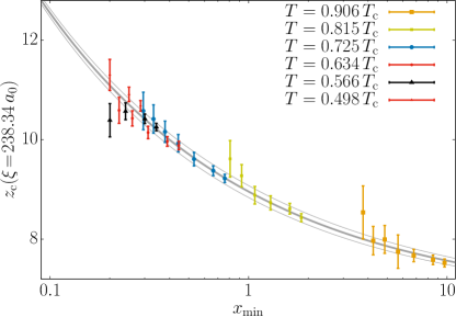
Figure 3: The estimates from different temperatures and minimal correlation lengths for the aging rate at $\xi_{\text{target}}=238.34~{}a_{0}$ (our largest) are a simple function of the crossover variable $x_{\text{min}}=\ell_{\text{J}}(T)/\xi_{\text{min}}$, see Eq. (7). The central black line is a fit to Eq. (7) with figure of merit $\chi^{2}/{\text{dof}}=24.5/30$ [dof = degrees of freedom. The fit generates the exponent $\beta(\xi_{\text{target}}=238.34~{}a_{0})=0.41$, the dependency on $\xi_{\text{target}}$ of exponent $\beta$ turns out to be small]. The upper (lower) black line is a fit to the data plus (minus) the error bar. The estimates of $z_{\mathrm{c}}$ for the different $(T,\xi_{\text{min}})$ were obtained by applying Eq. (6) to the data in Table III of the SM for Ref. Baity-Jesi et al. (2018) (see Appendix D for details).

IV Extrapolations from simulations.

The main problem to overcome is the crossover between critical scaling and the $T<T_{\mathrm{c}}$ Physics. Indeed, the largest correlation length reached in the simulations is $\xi=17.3\,a_{0}$ at $T=0.905T_{\mathrm{c}}$ Baity-Jesi et al. (2018), which results in a very large cross-over variable $x=1.96$. Much smaller values of $x$ were reached in the simulations, but at lower $T$ Baity-Jesi et al. (2018). Therefore, we need to consider the full data-set for $T<T_{\mathrm{c}}$ in Table III of the SM for Ref. Baity-Jesi et al. (2018). We shall only outline our analysis here and refer the reader to Appendix D for full details. To ease comparison with Baity-Jesi et al. (2018) , we give $\xi$ in units of $a_{0}$ from now on (recall that $a_{0}=0.64$ nm for our sample).

We should mention that two possibilities were considered in Ref. Baity-Jesi et al. (2018) for extrapolating the simulation’s $z_{\mathrm{c}}$ to larger values of $\xi$. One was Saclay’s ansatz for the crossover to activated dynamics Bouchaud et al. (2001); Berthier and Bouchaud (2002) which, however, yields too-high a $z_{\mathrm{c}}$ Baity-Jesi et al. (2018) when applied to the thin-film experiments Zhai et al. (2017). Therefore, we focus on the convergent ansatz for extrapolating $z_{\mathrm{c}}$ to correlation length $\xi_{\text{target}}$ by taking into account only data with $\xi\geq\xi_{\text{min}}$ ($\hat{\omega}=0.35$) Baity-Jesi et al. (2018)

$$z_{\mathrm{c}}(T,\xi_{\text{target}},\xi_{\text{min}})=\frac{T}{T_{\mathrm{c}}}\Big{[}z_{\infty}(T,\xi_{\text{min}})+\frac{A(T,\xi_{\text{min}})}{\xi_{\text{target}}^{\hat{\omega}}}\Big{]}\,.$$ (6)

Now, when applying Eq.(6) to any $\xi_{\text{target}}$, we end-up with as many predicted aging-rates as pairs of $(T,\xi_{\text{min}})$ were considered in the simulations. Fortunately, these many predictions, see Fig. 3, can be nicely organized as a function of the crossover variable $x_{\text{min}}=\ell_{\text{J}}(T)/\xi_{\text{min}}$ :

$$z_{\mathrm{c}}(T,\xi_{\text{target}},\xi_{\text{min}})=6.69+\frac{\alpha(\xi_{\text{target}})}{x_{\text{min}}^{\beta(\xi_{\text{target}})}}\,\,.$$ (7)

Thus, our final extrapolation at $T=28$ K is

$$z_{\mathrm{c}}(\xi_{\text{target}})=6.69+\frac{\alpha(\xi_{\text{target}})}{x_{\text{target}}^{\beta(\xi_{\text{target}})}}\,,\ x_{\text{target}}=\frac{\ell_{\text{J}}(28\text{K})}{\xi_{\text{target}}}\,,$$ (8)

[$\alpha(\xi_{\text{target}})$ and $\beta(\xi_{\text{target}})$ come from the fit to Eq. (7), recall Fig. 3]. We obtain in this way

$$z_{\mathrm{c}}(180.26\,a_{0})=11.94\pm 0.08\,,\ z_{\mathrm{c}}(238.34\,a_{0})=12.76\pm 0.08\,.$$ (9)

Both extrapolations are in excellent agreement with the experimental result $z_{c}=12.37\pm 1.07$ from Fig. 2 (roughly speaking, $z_{c}=12.37\pm 1.07$ is an average of $z_{\mathrm{c}}(\xi)$ in the range $180.26\,a_{0}\leq\xi\leq 238.34\,a_{0}$).

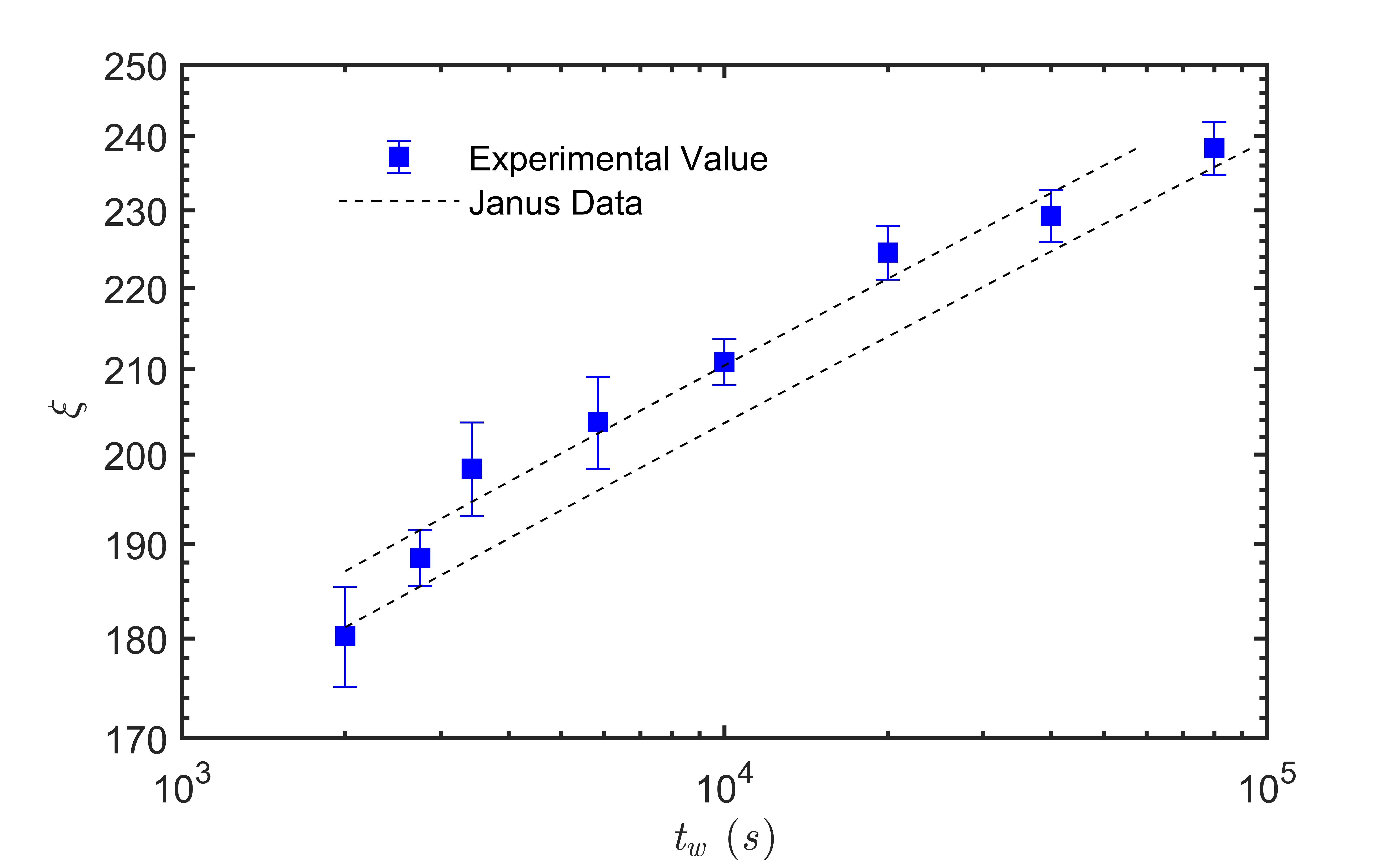
Figure 4: The experimental correlation length from Fig. 2, as measured in units of the average distance between magnetic moments $a_{0}=0.64$ nm, is shown as a function of the waiting time. The two continuous lines are obtained from our extrapolations from the simulations by the Janus collaboration Baity-Jesi et al. (2018), recall Eqs. (8,10). The two lines are the two extremal curves compatible with the initial condition taken from our experiment, $\xi^{*}(t_{\mathrm{w}}^{*}=2750\,\text{s})=(188.5\pm 3)\,a_{0}$.

We stress that the extrapolations (9) took no input from the experiment other than the values of $\xi_{\text{target}}$. However, by recalling [see Eq. (1)]

$$\ln\,t_{\mathrm{w}}-\ln\,t_{\mathrm{w}}^{*}=\int_{\ln\xi^{*}}^{\ln\xi}\,\mathrm{d}(\ln\xi^{\prime})\,\frac{T_{\mathrm{c}}}{T}z_{\mathrm{c}}(\xi^{\prime})\,,$$ (10)

and borrowing the initial condition $\xi^{*}(t_{\mathrm{w}}^{*}=2750\,\text{s})$ from the experiment, we obtain a fairly satisfactory comparison between our experiment and our extrapolations from the Janus simulations in Fig. 4. We note as well that the initial condition $\xi^{*}(t_{\mathrm{w}}=2000\,\text{s})$ from the experiment, afflicted by larger errors and short-time systematic effects, produces similar extrapolated curves.

V Conclusions.

We have reported an experimental measurement of the spin-glass correlation length in a single-crystal sample of CuMn (6 at.%). Our experiment is free from two systematic effects encountered in previous work: (i) the growth of the correlation length is not hampered by the sample geometry (neither crystallites Joh et al. (1999) or the film-thickness Zhai et al. (2017)) and (ii) our results are representative of the low-temperature phase (i.e. they are not contaminated by critical scaling), as shown by the small value of the cross-over variable we reach [recall Eq. (2)]. We report the largest spin-glass correlation length ever measured in a glassy phase. Our aging rate is also the largest to date (at least as measured in a spin-glass). We thus confirm the slowing down as $\xi$ grows that was suggested by the simulations of the Janus collaboration Baity-Jesi et al. (2018). Furthermore, we have been able to reproduce our experimental results by means of a simple extrapolation of the Janus results. We believe this relation between simulations and experiment opens new opportunities in condensed matter physics. The complementary contributions allow exploration of phenomena, especially in complex systems, with the particular insights of each partner fueling the interpretation and development of the other. This paper is the beginning of this new research relationship.

Appendix A Sample Preparation

Crystal growth and sample preparation was carried out by the Materials Preparation Center (MPC) of the Ames Laboratory, USDOE. Cu from Luvata Special Products (99.99 wt % with respect to specified elements) and distilled Mn from the MPC (99.93 wt% with respect to all elements) was arc melted several times under Ar and then drop cast in a water chilled copper mold. The resulting ingot was placed in a Bridgman style alumina crucible and heated under vacuum in a resistance Bridgman furnace to 1050⁰C, just above the melting point. The chamber was then backfilled to a pressure of 60 psi with high purity argon to minimize the vaporization of the Mn during the growth. The ingot was then further heated to 1300⁰C and held for one hour to ensure complete melting and time for the heat zone to reach a stable state. The ingot was withdrawn from the heat zone at a rate of 3mm/hr. About 1/3 of the crucible stuck to the alloy. The ingot was finally freed after alternating between hitting with a small punch and hammer and submerging in liquid nitrogen.

Cross-sections 1-2mm thick were taken from near the start of the crystal growth and from the end for characterization. One side of each was polished and looked at optically and with x-ray fluorescence (XRF). From the XRF measurements, the sample was found to be single phase and the end of the growth to be Mn rich. The samples were then etched in a 25% by volume solution of nitric acid in water. Optically, the start of the growth is a single phase, single crystal while the end of the growth has large grains with 2nd phase along the grain boundaries. Small pits were seen both optically and by XRF. The pits could be minimized by varying polishing techniques, but not gotten rid of. Fig. 5 displays the as-grown crystal.

Only the body portion of the crystal growth were used for the experiments. The ends of the growth were looked at as part of the characterization, but were not used because the end of the growth contained multiple grains and a second phase. An additional examination of the body waws done to ensure that enough of the bodyt had been cut away as to remove those unwanted elements. The small shallow grains that remained on one end of the body were avoided when cutting the sample to be measured. As mentioned above, the XRF showed the body of the crystal growthy to be single phase. The composition gradient is gradual and smooth, and there was no evidence of a Mn inhomogeneity seen in either the XRF or optical characterization.

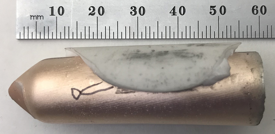
Figure 5: The as-grown crystal with part of the alumina crucible still attached. A small secondary grain is outlined with a marker. Later, acid etching of the ingot reduced the size and number of the secondary grains indicating that they are shallow.

Further investigation was done by polishing the cut ends of the ingot body followed by etching. No evidence of 2nd phase was seen and only occasional small, shallow secondary grains were found. In the Bridgman method, it is not unusual for the very end of the growth to be different because of accumulation of rejected elements and impurities ahead of the growth front. This would account for the change in growth habit (increased number of grains), presence of 2nd phase and overall Mn-rich composition seen at the end of the growth but not in the body. Laue x-ray diffraction along the length of the body, Fig. 6, confirms that the majority of the body is one single grain.

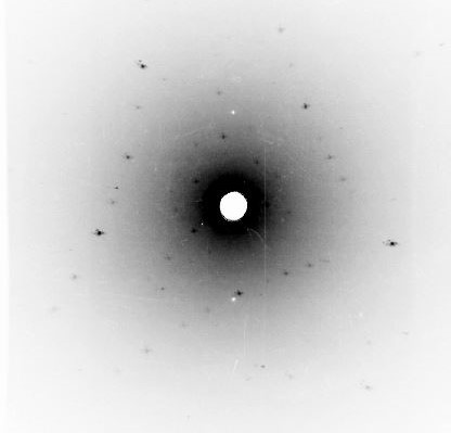
Figure 6: Laue x-ray diffraction pattern of the sample confirms it is a single crystal, the $\text{Cu}_{94}\text{Mn}_{6}$ cube sample was etched in 15% nitric acid. The 6 at.% Mn concentration was estimated from scaling using the observed temperature ($T_{g}=31.5$ K) at which the remanence disappeared.

Appendix B The parameters for computing the Josephson length

We follow here Ref. Baity-Jesi et al. (2018). The first step is converting the temperature to Janus units

$$T^{(J)}=\frac{T}{T_{\mathrm{c}}}T_{\mathrm{c}}^{(J)}\,\ T_{\mathrm{c}}^{(J)}=1.102\,.$$ (11)

Therefore, our working temperature $T=28K$ translates to $T^{(J)}=0.98$.

Next, we need to recall that the only thing we know for sure about this length scale is how it scales:

$$\ell_{\text{J}}(T^{(J)})=\frac{b_{0}+b_{1}(T_{\mathrm{c}}^{(J)}-T^{(J)})^{\nu}+b_{2}(T_{\mathrm{c}}^{(J)}-T^{(J)})^{\omega\nu}}{(T_{\mathrm{c}}^{(J)}-T^{(J)})^{-\nu}}$$ (12)

where we include analytic ($b_{1}$) and confluent ($b_{2})$ scaling corrections with $\omega=1.12(10)$, $\nu=2.56(4)$ and $T_{\mathrm{c}}^{(J)}=1.102(3)$ Baity-Jesi et al. (2013). Now, although there is no unique way of fixing the overall scale $b_{0}$ (only the quotients $b_{1}/b_{0}$ and $b_{2}/b_{0}$ can be fixed in an unique way), we shall adhere to the normalization of Ref. Baity-Jesi et al. (2018), so that we can compare to their data in a direct way:

$$b_{0} = 0.101507196509469\,,$$ (13)

$$b_{1} = 0.372545152960033\,,$$ (14)

$$b_{2} = 0.199692833647175\,.$$ (15)

With this convention for $b_{0}$, at the working temperature $T=0.98$ we have $\ell_{\text{J}}(0.98)=21.82\,a_{0}$.

Appendix C The replicon exponent and the self-consistent computation of $\xi$

Let us recall from the main text, the relation linking the number of correlated spins $N_{c}$ with the correlation length $\xi$:

$$N_{c}\approx\bigg{(}{\frac{\xi}{a_{0}}}\bigg{)}^{d_{f}}\,,$$ (16)

where $d_{f}$ is the fractal dimension equal to $d_{f}=d-\theta/2$ ($d=3$ is the space dimension, while $\theta$ is the so-called replicon exponent Baity-Jesi et al. (2017)). The quantity directly measured in the experiment is $Nc$, and our goal is to convert it into a length by using the fractal dimension.

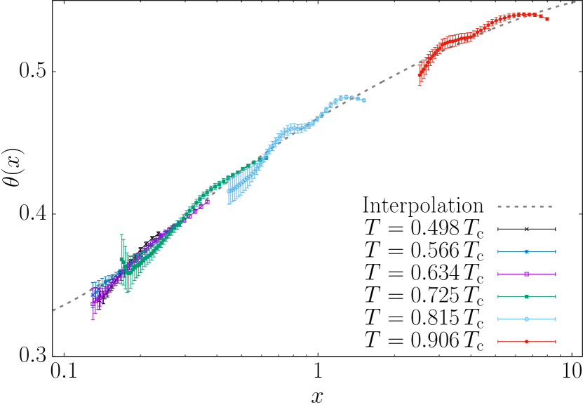
Figure 7: Data for the replicon exponent, taken from Fig. 5 in the Supplemental Material for Ref. Baity-Jesi et al. (2018), as a function of the crossover variable $x$ defined in Eq. (17). The black line is the RSB-inspired interpolation in Eq. (18). The wiggles are due to the extreme data-correlation (see, e.g, the discussion of Fig. 1 in Ref. Belletti et al. (2008)).

Now, the problem with Eq. (16) is that the replicon exponent, and hence $d_{f}$, depends on both the temperature and $\xi$ through the crossover variable (for the reader’s convenience, we repeat here thee definitions given in the main text):

$$x=\frac{\ell_{\text{J}}(T)}{\xi(t_{\mathrm{w}},T)}\,.$$ (17)

The data for $\theta(x(\xi,T))$, as well as a discussion of the asymptotic behavior for small $x$, are given in Sect. C of the Supplemental Material (SM) for Baity-Jesi et al. (2018). Here, we only observe that the numerical data for $\theta(x(\xi,T))$ are well interpolated as (see Fig. 7)

$$\theta(x)=\theta_{0}+d_{1}\Big{(}\frac{x}{1+e_{1}x}\Big{)}^{2-\theta_{0}}+d_{2}\Big{(}\frac{x}{1+e_{2}x}\Big{)}^{3-\theta_{0}}\,,$$ (18)

with numerical coefficients

$$\theta_{0}\ = 0.303980\,,$$ (19)

$$e_{1} = 1.38179\,,$$ (20)

$$d_{1} = 2.72489\,,$$ (21)

$$e_{2} = 2.12634\,,$$ (22)

$$d_{2} = -9.98359\,.$$ (23)

Let us emphasize that the interpolation 18 is consistent with the Replica Symmetry Breaking (RSB) asymptotic analysis (for small $x$) presented in the SM for Baity-Jesi et al. (2018). Yet, Eq. (18) can be applied as well for larger $x$ if needed.

Now, a droplets model supporter will object that $\theta_{0}$ should be zero (according to their theory). However, the RSB/droplets controversy is immaterial here: data can be fitted as well to the droplet model (see Baity-Jesi et al. (2018)), but the droplets fit start to depart significantly from the RSB interpolation in Eq. (18) only for $x<0.065$. Because we aim to use the interpolation in the range $x\geq 0.0915$, we do not need to care about the RSB/droplets controversy.

Figure 8: Self consistent computation of the replicon exponent $\theta$. By varying $\xi$, we obtain a parametric plot of $\theta=\theta(x=\ell_{\text{J}}(T=28K)/\xi)$, Eq. (18), as a function of the measured number of correlated spins $N_{c}$, see Eq. (24). The dots are the appropriate values of $\theta$ for our measured $N_{c}$. Note that $\theta$ is essentially constant in the experimentally relevant range of $Nc$.

After these preliminaries, the self-consistent computation is straightforward. In order to obtain $\theta$ as a function of the measured number of correlated spins $N_{c}$, see Fig. 8, we just need to vary $\xi$ parametrically and compute both $\theta(x=\ell_{\text{J}}(T=28K)/\xi)$ from Eq. (18) and $N_{c}$ from

$$N_{c}=(\xi/a_{0})^{d_{f}(x=\ell_{\text{J}}(28K)/\xi)}\,,d_{f}(x)=3-\frac{\theta{(x)}}{2}\,.$$ (24)

Appendix D Details on the extrapolation of the aging rate

Our basic quantity will be the (bare) aging-rate

$$z(T,\xi)=\frac{\mathrm{d}\,\ln\,t_{\mathrm{w}}}{\mathrm{d}\,\ln\,\xi}\,$$ (25)

(the renormalized aging-rate considered in the main text is just $z_{\text{c}}=zT/T_{\mathrm{c}}$).

Our starting point will be Table III in the Supplemental Material for Ref. Baity-Jesi et al. (2018). In this table, we find the extrapolated bare aging-rates for $\xi_{\text{target}}=38\,a_{0},76\,a_{0}$ and $\infty$, as computed from the convergent ansatz:

$$z(T,\xi_{\text{target}},\xi_{\text{min}})=z_{\infty}(T,\xi_{\text{min}})+\frac{A(T,\xi_{\text{min}})}{\xi_{\text{target}}^{\hat{\omega}}}\,.$$ (26)

In the above expression, $\hat{\omega}=0.35$ and $\xi_{\mathrm{min}}$ is the minimal correlation-length considered in their fit. It varies from varies from $\xi_{\mathrm{min}}=3.5\,a_{0}$ to $\xi_{\mathrm{min}}=9\,a_{0}$ (or less than $9\,a_{0}$ at the lowest temperatures).

Our first step was getting the slopes $A(T,\xi_{\text{min}})$ from the tabulated values for $\xi_{\text{target}}=38\,a_{0}$ and $76\,a_{0}$ (instead, $z_{\infty}(T,\xi_{\text{min}})$ is directly tabulated). With this information in our hands, we may compute $z(T,\xi_{\text{target}},\xi_{\text{min}})$ for any value of $\xi_{\text{target}}$ we wish. As for the error estimate, it is only slightly more complicated:

$$\Delta^{2}z(T,\xi_{\text{target}},\xi_{\text{min}}) = E_{11}^{(T,\xi_{\text{min}})}+E_{22}^{(T,\xi_{\text{min}})}\frac{1}{\xi_{\text{target}}^{2\hat{\omega}}}$$ (27)

$$+ E_{12}^{(T,\xi_{\text{min}})}\frac{1}{\xi_{\text{target}}^{\hat{\omega}}}\,.$$

Now, for every $T$ and $\xi_{\text{min}}$, we find error estimates for $\xi_{\text{target}}=\infty$, $76\,a_{0}$ and $38\,a_{0}$ in the table by the Janus Collaboration, which allows us to obtain the constants $E_{11}^{(T,\xi_{\text{min}})}$, $E_{22}^{(T,\xi_{\text{min}})}$. Once we have in our hands the coefficients $E_{22}^{(T,\xi_{\text{min}})}$, $E_{11}^{(T,\xi_{\text{min}})}$ and $E_{12}^{(T,\xi,\xi_{\text{min}})}$ we may compute errors for whatever value of $\xi_{\text{target}}$ we need by using Eq (27).

Our next step was obtaining $z(T,\xi_{\text{target}},\xi_{\text{min}})$ for a grid of values $180.26\,a_{0}\leq\xi_{\text{target}}\leq 238.34\,a_{0}$. We computed $z(T,\xi_{\text{target}},\xi_{\text{min}})$ for all the values of $(T,\xi_{\text{min}})$ in their Table III. We only neglected the few entries where the error for $z(T,\xi_{\text{target}}=\infty,\xi_{\text{min}})$ was well above $10\%$. Then, the estimates for the different $(T,\xi_{\text{min}})$ but the same $\xi_{\text{target}}$ were combined as explained, in the main text (recall that the renormalized aging rate is $z_{\mathrm{c}}=Tz/T_{\mathrm{c}}$) by means to a fit to:

$$z_{\mathrm{c}}(T,\xi_{\text{target}},\xi_{\text{min}})=6.69+\frac{\alpha(\xi_{\text{target}})}{x_{\text{min}}^{\beta(\xi_{\text{target}})}}\,\,,$$ (28)

where $x_{\text{min}}=\ell_{\text{J}}(T)/\xi_{\text{min}}$. Our final extrapolation was

$$z_{\mathrm{c}}(\xi_{\text{target}})=6.69+\frac{\alpha(\xi_{\text{target}})}{x_{\text{target}}^{\beta(\xi_{\text{target}})}}\,,\ x_{\text{target}}=\frac{\ell_{\text{J}}(28\text{K})}{\xi_{\text{target}}}\,.$$ (29)

The only tricky point needing further discussion regards the computation of errors in $z_{\mathrm{c}}(\xi_{\text{target}})$. It is clear that the different data in the fit are extremely correlated (at least those at the same temperature: in Table III of the SM for Ref. Baity-Jesi et al. (2018) the Janus collaboration was simply using the same set of $\xi(t_{\mathrm{w}},T)$ and discarding those with $\xi(t_{\mathrm{w}},T)<\xi_{\text{min}}$). Under such conditions, the fit’s standard errors are not reliable. Hence, in order to estimate errors, we simply repeated the fit for $z_{\mathrm{c}}(T,\xi_{\text{target}},\xi_{\text{min}})$ plus (or minus) the error. In other words, we assumed coherent fluctuations for all the data set. The errors quoted in the main text are the halved difference between the fit with data plus error and data minus error. A second, far more conservative error estimate, would be just taking the error from the data point at the lowest value of $x_{\text{min}}$ included in the fit to Eq. (28). The conservative error estimate is larger than the error from the halved-difference by a factor 3.75.

References

- Cavagna (2009) A. Cavagna, Physics Reports 476, 51 (2009) .
- Gunnarsson et al. (1991) K. Gunnarsson, P. Svedlindh, P. Nordblad, L. Lundgren, H. Aruga, and A. Ito, Phys. Rev. B 43, 8199 (1991).
- Adam and Gibbs (1965) G. Adam and J. H. Gibbs, The Journal of Chemical Physics 43, 139 (1965).
- Joh et al. (1999) Y. G. Joh, R. Orbach, G. G. Wood, J. Hammann, and E. Vincent, Phys. Rev. Lett. 82, 438 (1999).
- Albert et al. (2016) S. Albert, T. Bauer, M. Michl, G. Biroli, J.-P. Bouchaud, A. Loidl, P. Lunkenheimer, R. Tourbot, C. Wiertel-Gasquet, and F. Ladieu, Science 352, 1308 (2016) .
- Note (1) General theoretical arguments suggest that is also -independent at exactly Zinn-Justin (2005). Only if is -independent we have a power-law scaling . If grows with , as we find here, we encounter a dynamics slower than a power-law (for instance, an activated dynamics with free-energy barriers for some ).
- Zhai et al. (2017) Q. Zhai, D. C. Harrison, D. Tennant, E. D. Dalhberg, G. G. Kenning, and R. L. Orbach, Phys. Rev. B 95, 054304 (2017).
- Kenning et al. (2018) G. G. Kenning, D. M. Tennant, C. M. Rost, F. G. da Silva, B. J. Walters, Q. Zhai, D. C. Harrison, E. D. Dahlberg, and R. L. Orbach, Phys. Rev. B 98, 104436 (2018).
- Baity-Jesi et al. (2018) M. Baity-Jesi, E. Calore, A. Cruz, L. A. Fernandez, J. M. Gil-Narvion, A. Gordillo-Guerrero, D. Iñiguez, A. Maiorano, E. Marinari, V. Martin-Mayor, J. Moreno-Gordo, A. Muñoz Sudupe, D. Navarro, G. Parisi, S. Perez-Gaviro, F. Ricci-Tersenghi, J. J. Ruiz-Lorenzo, S. F. Schifano, B. Seoane, A. Tarancon, R. Tripiccione, and D. Yllanes (Janus Collaboration), Phys. Rev. Lett. 120, 267203 (2018).
- Baity-Jesi et al. (2014a) M. Baity-Jesi, R. A. Baños, A. Cruz, L. A. Fernandez, J. M. Gil-Narvion, A. Gordillo-Guerrero, D. Iniguez, A. Maiorano, F. Mantovani, E. Marinari, V. Martín-Mayor, J. Monforte-Garcia, A. Muñoz Sudupe, D. Navarro, G. Parisi, S. Perez-Gaviro, M. Pivanti, F. Ricci-Tersenghi, J. J. Ruiz-Lorenzo, S. F. Schifano, B. Seoane, A. Tarancon, R. Tripiccione, and D. Yllanes (Janus Collaboration), Comp. Phys. Comm 185, 550 (2014a) .
- Josephson (1966) B. D. Josephson, Phys. Lett. 21, 608 (1966).
- Baity-Jesi et al. (2013) M. Baity-Jesi, R. A. Baños, A. Cruz, L. A. Fernandez, J. M. Gil-Narvion, A. Gordillo-Guerrero, D. Iniguez, A. Maiorano, F. Mantovani, E. Marinari, V. Martín-Mayor, J. Monforte-Garcia, A. Muñoz Sudupe, D. Navarro, G. Parisi, S. Perez-Gaviro, M. Pivanti, F. Ricci-Tersenghi, J. J. Ruiz-Lorenzo, S. F. Schifano, B. Seoane, A. Tarancon, R. Tripiccione, and D. Yllanes (Janus Collaboration), Phys. Rev. B 88, 224416 (2013) .
- Bray and Moore (1982) A. J. Bray and M. A. Moore, J. Phys. C: Solid St. Phys. 15, 3897 (1982).
- Baity-Jesi et al. (2014b) M. Baity-Jesi, L. A. Fernandez, V. Martín-Mayor, and J. M. Sanz, Phys. Rev. 89, 014202 (2014b) .
- Amit and Martín-Mayor (2005) D. J. Amit and V. Martín-Mayor, Field Theory, the Renormalization Group and Critical Phenomena, 3rd ed. (World Scientific, Singapore, 2005).
- Guchhait and Orbach (2017) S. Guchhait and R. L. Orbach, Phys. Rev. Lett. 118, 157203 (2017).
- Wandersman et al. (2008) E. Wandersman, V. Dupuis, E. Dubois, R. Perzynski, S. Nakamae, and E. Vincent, EPL (Europhysics Letters) 84, 37011 (2008).
- Nair and Nigam (2007) S. Nair and A. K. Nigam, Phys. Rev. B 75, 214415 (2007).
- Baity-Jesi et al. (2017) M. Baity-Jesi, E. Calore, A. Cruz, L. A. Fernandez, J. M. Gil-Narvion, A. Gordillo-Guerrero, D. Iñiguez, A. Maiorano, E. Marinari, V. Martin-Mayor, J. Monforte-Garcia, A. Muñoz Sudupe, D. Navarro, G. Parisi, S. Perez-Gaviro, F. Ricci-Tersenghi, J. J. Ruiz-Lorenzo, S. F. Schifano, B. Seoane, A. Tarancon, R. Tripiccione, and D. Yllanes (Janus Collaboration), Phys. Rev. Lett. 118, 157202 (2017).
- Note (2) The reader will note that the right-hand side of Eq. (5) could be modified by a prefactor of order 1.This is why we are using an approximate sign in the equation, rather than an equal sign. However, the comparison with the simulations turns out to be satisfactory by assuming that the prefactor is exactly one. It is well possible that carrying out our program from future experiments of increased accuracy will require a more precise determination of this prefactor.
- Note (3) Amusingly, although the droplets model McMillan (1983); Bray and Moore (1987); Fisher and Huse (1986) and the Replica Symmetry Breaking (RSB) theory Marinari et al. (2000) differ in their expectation for (the droplets prediction is and , while RSB expects and ), the two theories quantitatively agree in their predicted behavior for in our range of Baity-Jesi et al. (2018).
- Bouchaud et al. (2001) J.-P. Bouchaud, V. Dupuis, J. Hammann, and E. Vincent, Phys. Rev. B 65, 024439 (2001).
- Berthier and Bouchaud (2002) L. Berthier and J.-P. Bouchaud, Phys. Rev. B 66, 054404 (2002).
- Note (4) Note that Eq. (7\@@italiccorr) correctly predicts , because at , for all .
- Belletti et al. (2008) F. Belletti, M. Cotallo, A. Cruz, L. A. Fernandez, A. Gordillo-Guerrero, M. Guidetti, A. Maiorano, F. Mantovani, E. Marinari, V. Martín-Mayor, A. M. Sudupe, D. Navarro, G. Parisi, S. Perez-Gaviro, J. J. Ruiz-Lorenzo, S. F. Schifano, D. Sciretti, A. Tarancon, R. Tripiccione, J. L. Velasco, and D. Yllanes (Janus Collaboration), Phys. Rev. Lett. 101, 157201 (2008) .
- Zinn-Justin (2005) J. Zinn-Justin, Quantum Field Theory and Critical Phenomena, 4th ed. (Clarendon Press, Oxford, 2005).
- McMillan (1983) W. L. McMillan, Phys. Rev. B 28, 5216 (1983).
- Bray and Moore (1987) A. J. Bray and M. A. Moore, in Heidelberg Colloquium on Glassy Dynamics, Lecture Notes in Physics No. 275, edited by J. L. van Hemmen and I. Morgenstern (Springer, Berlin, 1987).
- Fisher and Huse (1986) D. S. Fisher and D. A. Huse, Phys. Rev. Lett. 56, 1601 (1986).
- Marinari et al. (2000) E. Marinari, G. Parisi, F. Ricci-Tersenghi, J. J. Ruiz-Lorenzo, and F. Zuliani, J. Stat. Phys. 98, 973 (2000) .