Model based fractional order controller design for process plants satisfying desired robustness criteria

Abstract

This paper contributes to the design of a fractional order (FO) internal model controller (IMC) for a first order plus time delay (FOPTD) process model to satisfy a given set of desired robustness specifications in terms of gain margin $(A_{m})$ and phase margin $(\phi_{m})$. The highlight of the design is the choice of a fractional order (FO) filter in the IMC structure which has two parameters ($\lambda$ and $\beta$) to tune as compared to only one tuning parameter ($\lambda$) for traditionally used integer order (IO) filter. These parameters are evaluated for the controller, so that $A_{m}$ and $\phi_{m}$ can be chosen independently. A new methodology is proposed to find a complete solution for controller parameters, the methodology also gives the system gain cross-over frequency ($\omega_{g}$) and phase cross-over frequency ($\omega_{p}$). Moreover, the solution is found without any approximation of the delay term appearing in the controller.

Keywords Internal Model Control, fractional order control, gain margin, phase margin, first order plus time delay process model.

1 Introduction

The IMC control strategy was proposed by M.Morari et al. in 1982 [1, 2]. The IMC control structure as shown in Fig.1(a) constitutes the inverse of the minimum phase part of the process model $\hat{G}_{m}(s)$ which is augmented with a filter $\Theta(s)$ and is given as $Q(s)=\hat{G}_{m}(s)/\Theta(s)$ [3], such that $\mathop{\lim}\limits_{\omega\to 0}\Theta(j\omega)=1$. Usually the filter is considered as $\Theta(s)=1/(\lambda s+1)^{r}$ where $r$ is so chosen that $Q(s)$ becomes bi-proper. The parameter $\lambda$ is used to tune the controller to get the desired closed loop response of the system [3]. This is the standard IO filter design problem for the IMC, where any value of $\lambda$ in the filter provides some $A_{m}$ and $\phi_{m}$ to the closed loop system, or in other words, for desired $A_{m}$ and $\phi_{m}$, parameter $\lambda$ is evaluated.

To the best of author’s knowledge, only two major contributions [4, 5] are present in literature which design IMC controller to satisfy $A_{m}$ and $\phi_{m}$ specifications simultaneously, whereas [6] implemented the work in [5] in adaptive control setting. All three of them are IO-IMC for FOPTD processes.

The major limitation of these controllers is the presence of only one tuning parameter $\lambda$ which limits the domain of selection of desired $A_{m}$ and $\phi_{m}$. The achievable $A_{m}$ and $\phi_{m}$ are related through a mathematical expression which represents a curve (say, $A_{m}-\phi_{m}$ curve) in a 2-D space and desired $A_{m}$ and $\phi_{m}$ can be selected from that curve only. Also, the possible $\phi_{m}$ is restricted to $(0,\pi/2)$.

To overcome these issues an FO filter $\Theta(s)=1/(\lambda s^{\beta}+1)$ is considered in this work which introduces an additional parameter $\beta$ into the controller. With two tuning parameters $(\lambda,\beta)$ instead of only $\lambda$ as in IO filter, the range of selection of desired $A_{m}$ and $\phi_{m}$ becomes a 2-D surface and hence it becomes possible to select $A_{m}$ and $\phi_{m}$ independently..

In this paper, a new solution method is developed to simultaneously satisfy $A_{m}\geq 2$ and $\phi_{m}\in(0,\pi)$ for $\theta/\tau>0$, where $\theta$ is the delay and $\tau$ is the time constant of the plant, for FOPTD processes. The methodology also provides the solution of the system $\omega_{g}$ and $\omega_{p}$ considering them as the transitional variable. It is also the first time that, the solution is attempted without any approximation of the delay term in the controller.

The contents of this manuscript are as follows: Section-II contains complete controller design methodology, derivations, proofs and controller design steps. Section-III, analysis on disturbance rejection with the proposed controller is given. The proposed methodology is verified with an example in Section-IV and Section-V is dedicated to discussion and conclusions.

2 Internal Model Controller

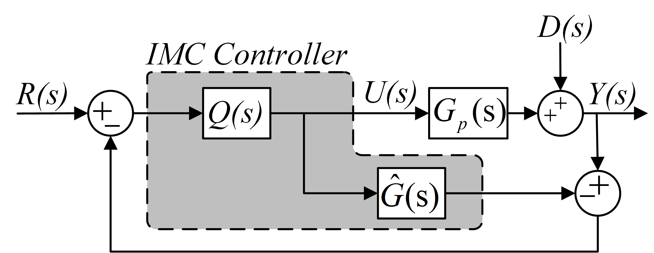
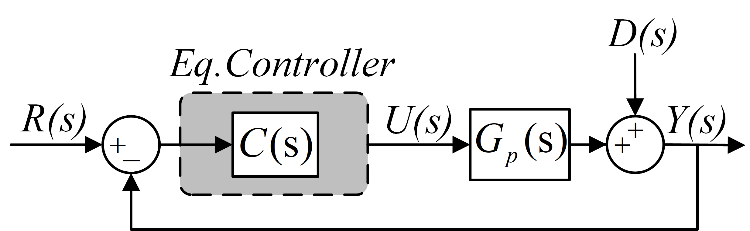
Figure 1: (a) IMC control and (b) Equivalent classical control

In Fig.1(a), $Q(s)$ is the IMC controller, ${G_{p}}(s)$ is the process and $\hat{G}(s)$ is the model of the process used in the control loop. In Fig.1(b), $C(s)$ is the equivalent classical controller obtained by block diagram reduction in the structure of Fig.1(a) and is given as $C(s)=Q(s)/(1-Q(s)\hat{G}(s))$. Assuming plant behavior as FOPTD and exact modeling as per [3], $\hat{G}(s)$ can be written as

$$\hat{G}(s)=G_{p}(s)=\frac{k}{\tau s+1}e^{-\theta s}$$ (1)

Segregating the minimum phase (MP) and non-minimum phase (NMP) part of the process and the model, we have $G_{p}(s)=G_{pm}(s)G_{pa}(s)$ and $\hat{G}(s)=\hat{G}_{m}(s)\hat{G}_{a}(s)$, where subscript ${}^{\prime}a^{\prime}$ represents NMP or all-pass part and subscript ${}^{\prime}m^{\prime}$ represents MP part of the transfer function. Since $\hat{G}(s)=G_{p}(s)$ therefore,

$$\hat{G}_{m}(s)=G_{pm}(s)=\frac{k}{\tau s+1};\qquad\hat{G}_{a}(s)=G_{pa}(s)=e^{-\theta s}$$ (2)

The IMC controller $Q(s)$ is given as [3]

$$Q(s)=\frac{\Theta(s)}{{\hat{G}_{m}}(s)}$$ (3)

where $\Theta(s)$ is an FO filter chosen in such a way that $Q(s)$ is realizable and $\mathop{\lim}\limits_{s\to 0}{\Theta}(s)=1$ [3]. The FO filter considered in this paper is

$$\Theta(s)=\frac{1}{{\lambda{s^{\beta}}+1}};\quad\beta\in(0,2),\,\lambda>0$$ (4)

where $\beta$ denoting the fractional order is an additional parameter along with the filter constant $\lambda$.

2.1 $A_{m}$ and $\phi_{m}$ specifications:

Substituting $\hat{G}_{m}(s)$ from (2) and $\Theta(s)$ from (4) in (3), we get

$$Q(s)=\frac{\tau s+1}{k(\lambda s^{\beta}+1)}$$ (5)

The equivalent controller in Fig.1(b) can be obtained by substituting $Q(s)$ from (5) and $\hat{G}(s)$ from (1) in $C(s)=Q(s)/(1-Q(s)\hat{G}(s))$, and we get

$$C(s)=\frac{1}{{\lambda{s^{\beta}}+1-{e^{-\theta s}}}}\cdot\frac{1}{{{{\hat{G}}_{m}}(s)}}$$ (6)

The open loop transfer function based on Fig.1(b) is $L(s)=C(s)G_{p}(s)$ considering $D(s)=0$, since $D(s)$ has no influence on the $A_{m}$ and $\phi_{m}$ specifications. Substituting $C(s)$ from (6) and $G_{p}(s)$ from (1), the open loop transfer function (OLTF) becomes

$$L(s)=\frac{{{e^{-\theta s}}}}{{\lambda{s^{\beta}}+1-{e^{-\theta s}}}}$$ (7)

For an OLTF $L(s)$, the $A_{m}$ and $\phi_{m}$ specifications are given as

$${\left.{L(j\omega)}\right|_{\omega={\omega_{g}}}}=-{e^{j{\phi_{m}}}}$$ (8)

$$\qquad{\left.{L(j\omega)}\right|_{\omega={\omega_{p}}}}=\frac{{-1}}{{{A_{m}}}}$$ (9)

where $\omega_{g}$ is gain cross-over frequency and $\omega_{p}$ is phase cross-over frequency of the closed loop system. To have desired $A_{m}$ and $\phi_{m}$, we need to find $\lambda$ and $\beta$ which satisfy (8) and (9) simultaneously. Substituting $s=j\omega$ in (7), we get

$$L(j\omega)=\frac{{{e^{-j\theta\omega}}}}{\begin{array}[]{c}\left({1+\lambda{\omega^{\beta}}\cos\left({\frac{{\beta\pi}}{2}}\right)-\cos\left({\theta\omega}\right)}\right)+j\left({\lambda{\omega^{\beta}}\sin\left({\frac{{\beta\pi}}{2}}\right)+\sin\left({\theta\omega}\right)}\right)\end{array}}$$ (11)

Form (11) and (8), we have

$$\begin{array}[]{*{20}{c}}\begin{array}[]{c}\Rightarrow\left({1+\lambda\omega_{g}^{\beta}\cos\left({\frac{{\beta\pi}}{2}}\right)-\cos\left({\theta{\omega_{g}}}\right)}\right)+j\left({\lambda\omega_{g}^{\beta}\sin\left({\frac{{\beta\pi}}{2}}\right)+\sin\left({\theta{\omega_{g}}}\right)}\right)\end{array}&{=-{e^{-j\left({{\phi_{m}}+\theta{\omega_{g}}}\right)}}}\end{array}$$

$$\begin{array}[]{c}\Rightarrow\left({1+\lambda\omega_{g}^{\beta}\cos\left({\frac{{\beta\pi}}{2}}\right)-\cos\left({\theta{\omega_{g}}}\right)}\right)+j\left({\lambda\omega_{g}^{\beta}\sin\left({\frac{{\beta\pi}}{2}}\right)+\sin\left({\theta{\omega_{g}}}\right)}\right)=-\cos\left({{\phi_{m}}+\theta{\omega_{g}}}\right)+j\sin\left({{\phi_{m}}+\theta{\omega_{g}}}\right)\end{array}$$ (13)

Equating real and imaginary part in (13), we get

$${1+\lambda\omega_{g}^{\beta}\cos\left({\frac{{\beta\pi}}{2}}\right)-\cos\left({\theta{\omega_{g}}}\right)}=-\cos\left({{\phi_{m}}+\theta{\omega_{g}}}\right)$$ (14)

$$\text{and}\qquad\lambda\omega_{g}^{\beta}\sin\left({\frac{{\beta\pi}}{2}}\right)+\sin\left({\theta{\omega_{g}}}\right)=\sin\left({{\phi_{m}}+\theta{\omega_{g}}}\right)$$ (15)

Similarly, from (11) and (9) we get

$$\begin{array}[]{*{20}{c}}\left({1+\lambda\omega_{p}^{\beta}\cos\left({\frac{{\beta\pi}}{2}}\right)-\cos\left({\theta{\omega_{p}}}\right)}\right)+j\left({\lambda\omega_{p}^{\beta}\sin\left({\frac{{\beta\pi}}{2}}\right)+\sin\left({\theta{\omega_{p}}}\right)}\right)=-{A_{m}}{e^{-j\theta{\omega_{p}}}}\end{array}$$

$$\Rightarrow\left({1+\lambda\omega_{p}^{\beta}\cos\left({\frac{{\beta\pi}}{2}}\right)-\cos\left({\theta{\omega_{p}}}\right)}\right)+j\left({\lambda\omega_{p}^{\beta}\sin\left({\frac{{\beta\pi}}{2}}\right)+\sin\left({\theta{\omega_{p}}}\right)}\right)=-{A_{m}}\cos\left({\theta{\omega_{p}}}\right)+j{A_{m}}\sin\left({\theta{\omega_{p}}}\right)$$ (16)

Equating real and imaginary part in (16), we get

$$1+\lambda\omega_{p}^{\beta}\cos\left({\frac{{\beta\pi}}{2}}\right)-\cos\left({\theta{\omega_{p}}}\right)=-{A_{m}}\cos\left({\theta{\omega_{p}}}\right)$$ (17)

$$\text{and}\qquad{\lambda\omega_{p}^{\beta}\sin\left({\frac{{\beta\pi}}{2}}\right)+\sin\left({\theta{\omega_{p}}}\right)}={A_{m}}\sin\left({\theta{\omega_{p}}}\right)$$ (18)

The problem has four non-linear transcendental equations (14), (15), (17), and (18) with four unknowns $\lambda$, $\beta$, $\omega_{g}$ & $\omega_{p}$, where $\lambda$ and $\beta$ are to be evaluated such that the desired $\phi_{m}$ and $A_{m}$ are satisfied simultaneously, $\omega_{g}$ and $\omega_{p}$ begin transitional variables. The solution of equations (14) and (15) shall give $\lambda$ and $\beta$ such that it satisfies (8) or in other words it satisfies $\phi_{m}$ and $\omega_{g}$ simultaneously. Similarly, solution of equations (17) and (18) shall give the values of $\lambda$ and $\beta$ such that it satisfies (9) or equivalently, it satisfies $A_{m}$ and $\omega_{p}$ simultaneously.

2.2 Design Philosophy:

Let us denote $\lambda=\lambda_{a}$ in (13). Then $\lambda$ in (14) and (15) becomes $\lambda_{a}$ as they come from the same equation (13). Similarly, denoting $\lambda=\lambda_{b}$ in (16), $\lambda$ in (17) and (18) becomes $\lambda_{b}$.

Then the solution of (14) and (15) would give a set $\Delta_{a}$, containing $\{\lambda_{a},\beta_{\omega_{g}}\}$ corresponding to a set $\Xi_{a}$ which contains those $\{\phi_{m},\omega_{g}\}$ which satisfy (13). Similarly, the solution of (17) and (18) will give a set $\Delta_{b}$, containing $\{\lambda_{b},\beta_{\omega_{p}}\}$ corresponding to a set $\Xi_{b}$ which contains those $\{A_{m},\omega_{p}\}$ which satisfy (16). Then the intersection set $\Delta_{c}=\Delta_{a}\cap\Delta_{b}$ shall contain $\{\lambda_{c}^{\star},\beta_{c}^{\star}\}$ which satisfy both (13) and (16), for a given $\{A_{m}^{\star},\phi_{m}^{\star}\}$, where $A_{m}^{\star}$ and $\phi_{m}^{\star}$ are elements from the set $\Xi_{c}=\Xi_{a}\cap\Xi_{b}$ associated with some corresponding $\omega_{p}^{*}$ and $\omega_{g}^{*}$.

To obtain the solution, first we assume $\beta_{\omega_{g}}=\beta\in(0,2)$ and find corresponding $\omega_{g}$ in terms of $\beta_{{\omega_{g}}}$ from (14) and (15) by eliminating $\lambda_{a}$. Substituting this $\{\omega_{g},\beta_{{\omega_{g}}}\}$ in (14) or (15), we get corresponding $\lambda_{a}$ values. Similarly we consider $\beta_{\omega_{p}}=\beta\in(0,2)$ and find $\omega_{p}$ in terms of $\beta_{{\omega_{p}}}$ from (17) and (18) by eliminating $\lambda_{b}$. Substituting this $\{\omega_{p},\beta_{{\omega_{p}}}\}$ in (17) or (18), we get corresponding $\lambda_{b}$. Therefore, $\{\lambda_{a},\beta_{\omega_{g}}\}$ lead to a set $\Xi_{a}$ which contains all $\{\phi_{m},\omega_{g}\}$ which $\{\lambda_{a},\beta_{\omega_{g}}\}$ can satisfy. Similarly, $\{\lambda_{b},\beta_{{\omega_{p}}}\}$ lead to a set $\Xi_{b}$ which contains all $\{A_{m},\omega_{p}\}$ which $\{\lambda_{b},\beta_{\omega_{p}}\}$ can satisfy. Then $\beta_{\omega_{g}}vs.\lambda_{a}$ and $\beta_{\omega_{p}}vs.\lambda_{b}$ are plotted together to find the intersection of the curve which gives $\lambda^{\star}$ and $\beta^{\star}$ which satisfies $\phi_{m}^{\star}$ at some $\omega_{g}^{\star}$ and $A_{m}^{\star}$ at some $\omega_{p}^{\star}$.

2.3 Finding $\omega_{g}\in\Xi_{a}$:

Eliminating $\lambda$ from (14) and (15), we get

$$\tan\left({\frac{{\beta\pi}}{2}}\right)=\frac{{\sin\left({{\phi_{m}}+\theta{\omega_{g}}}\right)-\sin\left({\theta{\omega_{g}}}\right)}}{{\cos\left({\theta{\omega_{g}}}\right)-\cos\left({{\phi_{m}}+\theta{\omega_{g}}}\right)-1}}$$ (19)

In (19), $\beta$ and $\omega_{g}$ are unknown, whereas $\phi_{m}$ is given as the desired phase margin and $\theta$ is given from the system model. However, since the range of $\beta$ is fixed, therefore, $\omega_{g}$ can be found in terms of $\beta$.

Cross multiplying with numerator and denominator terms in LHS and RHS of the equation in (19), we get

$$\begin{array}[]{c}\tan\left({\frac{{\beta\pi}}{2}}\right)\cos\left({\theta{\omega_{g}}}\right)-\tan\left({\frac{{\beta\pi}}{2}}\right)\cos\left({{\phi_{m}}+\theta{\omega_{g}}}\right)-\tan\left({\frac{{\beta\pi}}{2}}\right)=\sin\left({{\phi_{m}}+\theta{\omega_{g}}}\right)-\sin\left({\theta{\omega_{g}}}\right)\end{array}$$ (21)

Using trigonometric identities and simplifying, we can write (21) as

$$a_{1}\cos\left({\theta{\omega_{g}}}\right)+b_{1}\sin\left({\theta{\omega_{g}}}\right)=c_{1}$$ (22)

where

$$\begin{array}[]{*{20}{c}}{{a_{1}}=\tan\left({\frac{{\beta\pi}}{2}}\right)\left({1-\cos\left({{\phi_{m}}}\right)}\right)-\sin\left({{\phi_{m}}}\right)};\,{{b_{1}}=\tan\left({\frac{{\beta\pi}}{2}}\right)\sin\left({{\phi_{m}}}\right)+\left({1-\cos\left({{\phi_{m}}}\right)}\right)};\,{{c_{1}}=\tan\left({\frac{{\beta\pi}}{2}}\right)}\end{array}$$ (24)

In (22), let $a_{1}=r_{1}\cos(\alpha_{1})$ & $b_{1}=r_{1}\sin(\alpha_{1})$ where $\alpha_{1}\in\Re$ and $\alpha_{1}$ is in radians. Then, $r_{1}=\sqrt{a_{1}^{2}+b_{1}^{2}}$ and $\alpha_{1}=\tan^{-1}\left(\frac{b_{1}}{a_{1}}\right)$. This transforms (22) as

$$\cos\left({\alpha_{1}-\theta{\omega_{g}}}\right)=\frac{c_{1}}{r_{1}}$$ (25)

Note that $\alpha_{1}$, $c_{1}$ and $r_{1}$ ultimately depend only on $\beta$.

Lemma 2.3.1 (Simplification for $c_{1}/r_{1}$)

If $a_{1}$, $b_{1}$ and $c_{1}$ are as given in (24), then

$$\frac{c_{1}}{r_{1}}=\frac{{\sin\left({\frac{{\beta\pi}}{2}}\right)}}{{2\sin\left({\frac{{{\phi_{m}}}}{2}}\right)}};\quad\beta\in\left({0,2}\right)$$ (26)

Proof 2.3.1

Substituting $a_{1}$ and $b_{1}$ from (24), and further simplification of the trigonometric terms, we get

$${a_{1}^{2}}+{b_{1}^{2}}={\left({\frac{{2\sin\left({\frac{{{\phi_{m}}}}{2}}\right)}}{{\cos\left({\frac{{\beta\pi}}{2}}\right)}}}\right)^{2}}$$ (27)

Hence $r_{1}=\sqrt{a_{1}^{2}+b_{1}^{2}}=\frac{{2\sin\left({\frac{{{\phi_{m}}}}{2}}\right)}}{{\cos\left({\frac{{\beta\pi}}{2}}\right)}}$. Then $\frac{c_{1}}{r_{1}}=\frac{{\sin\left({\frac{{\beta\pi}}{2}}\right)}}{{2\sin\left({\frac{{{\phi_{m}}}}{2}}\right)}}$.

From (26), it is clear that $\phi_{m}=0$ is not possible as at $\phi_{m}=0$, $c_{1}/r_{1}\to\infty$ and for such case the solution of $\omega_{g}$ from (25) does not exist.

Lemma 2.3.2 (Simplification for $\alpha_{1}$)

If $a_{1}$ and $b_{1}$ are as given in (24), then

$$\alpha_{1}=\left\{{\begin{array}[]{*{20}{c}}{-\left({\frac{{\beta\pi}}{2}+\frac{{{\phi_{m}}}}{2}}\right)}&{\color[rgb]{0,0,0}{\frac{{\beta\pi}}{2}+\frac{{{\phi_{m}}}}{2}\in\left({0,\frac{\pi}{2}}\right)}}\\ {\pi-\left({\frac{{\beta\pi}}{2}+\frac{{{\phi_{m}}}}{2}}\right)}&{\frac{{\beta\pi}}{2}+\frac{{{\phi_{m}}}}{2}\in\left({\frac{\pi}{2},\frac{{3\pi}}{2}}\right)}\end{array}}\right.$$ (28)

Proof 2.3.2

Since $\alpha_{1}=\tan^{-1}{b_{1}}/{a_{1}}$, substituting $a_{1}$ and $b_{1}$ from (24), and using trigonometric identities for simplification, we get

$$\alpha_{1}={\tan^{-1}}\left({\frac{{\tan\left({\frac{{\beta\pi}}{2}}\right)+\tan\left({\frac{{{\phi_{m}}}}{2}}\right)}}{{\tan\left({\frac{{\beta\pi}}{2}}\right)\tan\left({\frac{{{\phi_{m}}}}{2}}\right)-1}}}\right)$$

Therefore,

$$\alpha_{1}={\tan^{-1}}\left({-\tan\left({\frac{{\beta\pi}}{2}+\frac{{{\phi_{m}}}}{2}}\right)}\right)=-{\tan^{-1}}\left({\tan\left({\frac{{\beta\pi}}{2}+\frac{{{\phi_{m}}}}{2}}\right)}\right)$$ (29)

From fundamentals of inverse trigonometry, ${\tan^{-1}}\left({\tan\left(x\right)}\right)=x$, only if $x\in(-\pi/2,\pi/2)$. If $x$ lies outside this range, the origin needs to be shifted to the desired domain of the argument $x$ to get the correct result. Therefore, we obtain

$$\alpha_{1}=\left\{{\begin{array}[]{*{20}{c}}{-\left({\frac{{\beta\pi}}{2}+\frac{{{\phi_{m}}}}{2}}\right)}&{\frac{{\beta\pi}}{2}+\frac{{{\phi_{m}}}}{2}\in\left({0,\frac{\pi}{2}}\right)}\\ {\pi-\left({\frac{{\beta\pi}}{2}+\frac{{{\phi_{m}}}}{2}}\right)}&{\frac{{\beta\pi}}{2}+\frac{{{\phi_{m}}}}{2}\in\left({\frac{\pi}{2},\frac{{3\pi}}{2}}\right)}\end{array}}\right.$$

Theorem 2.3.1 (Solution of $\omega_{g}$)

The gain cross-over frequency $\omega_{g}$ which satisfies (8) can be found as

$${\omega_{g}}=\left\{{\begin{array}[]{*{20}{c}}{\frac{1}{\theta}\left({-{{\cos}^{-1}}\left({\frac{{\sin\left({\frac{{\beta\pi}}{2}}\right)}}{{2\sin\left({\frac{{{\phi_{m}}}}{2}}\right)}}}\right)-\left({\frac{{\beta\pi}}{2}+\frac{{{\phi_{m}}}}{2}}\right)}\right)}\\ {\color[rgb]{0,0,0}{;\;\beta\in\left({0,{\beta_{x1}}}\right)}}\\ {\frac{1}{\theta}\left({-{{\cos}^{-1}}\left({\frac{{\sin\left({\frac{{\beta\pi}}{2}}\right)}}{{2\sin\left({\frac{{{\phi_{m}}}}{2}}\right)}}}\right)+\pi-\left({\frac{{\beta\pi}}{2}+\frac{{{\phi_{m}}}}{2}}\right)}\right)}\\ {;\;\beta\in\left({{\beta_{x1}},{\beta_{x3}}}\right)}\end{array}}\right.$$ (30)

where ${{\beta_{x1}}}=(\pi-\phi_{m})/\pi$ and ${{\beta_{x3}}}=(3\pi-\phi_{m})/\pi$.

Proof 2.3.3

From (25), $\omega_{g}$ becomes

$${\omega_{g}}=\frac{1}{\theta}\left\{{-{{\cos}^{-1}}\left({\frac{{{c_{1}}}}{{{r_{1}}}}}\right)+{\alpha_{1}}}\right\}$$ (31)

Substituting $\cos^{-1}(c_{1}/r_{1})$ from (26) and $\alpha_{1}$ from (28) in (31), $\omega_{g}$ is given as

$${\omega_{g}}=\left\{{\begin{array}[]{*{20}{c}}{\frac{1}{\theta}\left({-{{\cos}^{-1}}\left({\frac{{\sin\left({\frac{{\beta\pi}}{2}}\right)}}{{2\sin\left({\frac{{{\phi_{m}}}}{2}}\right)}}}\right)-\left({\frac{{\beta\pi}}{2}+\frac{{{\phi_{m}}}}{2}}\right)}\right)}\\ {\color[rgb]{0,0,0}{;\;\frac{{\beta\pi}}{2}+\frac{{{\phi_{m}}}}{2}\in\left({0,\frac{\pi}{2}}\right)}}\\ {\frac{1}{\theta}\left({-{{\cos}^{-1}}\left({\frac{{\sin\left({\frac{{\beta\pi}}{2}}\right)}}{{2\sin\left({\frac{{{\phi_{m}}}}{2}}\right)}}}\right)+\pi-\left({\frac{{\beta\pi}}{2}+\frac{{{\phi_{m}}}}{2}}\right)}\right)}\\ {;\;\frac{{\beta\pi}}{2}+\frac{{{\phi_{m}}}}{2}\in\left({\frac{\pi}{2},\frac{{3\pi}}{2}}\right)}\end{array}}\right.$$ (32)

Simplifying the domain in (32) for $\beta$, we get $\beta\in{\color[rgb]{0,0,0}(-\phi_{m}/\pi,(\pi-\phi_{m})/\pi)}$ for the first case and $\beta\in((\pi-\phi_{m})/\pi,(3\pi-\phi_{m})/\pi)$ for the second case. However, $\beta\in(0,2)$ therefore, the lower bound for the first case will become zero. Therefore, the first domain will become $\beta\in{\color[rgb]{0,0,0}(0,\beta_{x1})}$ and the second domain remains as it is, i.e., $\beta\in(\beta_{x1},\beta_{x3})$.

2.4 Finding $\beta_{\omega_{g}}$ from set $\Xi_{a}$:

In practice, control systems always have real and positive gain cross-over frequency. Let ${\rm B}_{\omega_{g}}$ be the set of $\beta$ which gives some desired $\omega_{g}$ which is real and positive, i.e, ${{\rm B}_{\omega_{g}}}=\left\{{\beta:{\omega_{g}}\in{\Re^{+}}}\right\}$.

From (32), the solution of $\omega_{g}$ depends on $\beta$ and $\phi_{m}$. However, $\phi_{m}$ is given by design specification, therefore, $\beta$ can be found in terms of $\phi_{m}$ such that $\omega_{g}\in\Re^{+}$. This can be done in two steps. First, $\beta$ is obtained so that $\omega_{g}\in\Re$, i.e., set ${{\rm B}_{\omega g\Re}}=\left\{{\beta:{\omega_{g}}\in\Re}\right\}$ is evaluated. Thereafter, set ${{\rm B}_{\omega g+}}=\left\{{\beta:{\omega_{g}}>0}\right\}$ is obtained. Finally, ${{\rm B}_{\omega g}}={{\rm B}_{\omega g\Re}}\cap{{\rm B}_{\omega g+}}$.

Theorem 2.4.1 ( Finding $\rm B_{\omega_{g}\Re}$)

If $c_{1}/r_{1}$ is as given in (26), then the solution of $\beta$ such that $\omega_{g}\in\Re$ is given by:
(a) ${{\rm B}_{{\omega_{g}}\Re}}=\left\{{\beta:\beta\in(0,{\beta_{{\omega_{g}}\Re 1}})\cup({\beta_{{\omega_{g}}\Re 2}},2)}\right\}$ when $\phi_{m}\in(0,\pi/3)$ and
(b) ${{\rm B}_{{\omega_{g}}\Re}}=\left\{{\beta:\beta\in(0,2)}\right\}$ when $\phi_{m}\in[\pi/3,\pi)$, where

$${\beta_{{\omega_{g}}\Re 1}}=\frac{2}{\pi}{\sin^{-1}}\left({2\sin\left({\frac{{{\phi_{m}}}}{2}}\right)}\right)$$ (33)

$$and\qquad{{\beta_{{\omega_{g}}\Re 2}}=\frac{2}{\pi}\left({\pi-{{\sin}^{-1}}\left({2\sin\left({\frac{{{\phi_{m}}}}{2}}\right)}\right)}\right)}$$ (34)

Proof 2.4.1

From (31), $\omega_{g}\in\Re$ if $\left|c_{1}/r_{1}\right|\leq 1$, where $c_{1}/r_{1}$ is given in (26). Thus,

$$\left|{\frac{{\sin\left({\frac{{\beta\pi}}{2}}\right)}}{{2\sin\left({\frac{{{\phi_{m}}}}{2}}\right)}}}\right|\leq 1$$ (35)

Since $c_{1}/r_{1}>0\,\forall\,\beta\in(0,2)$ and $\phi_{m}\in(0,\pi)$, therefore, modulus sign can be removed from (35), and we get

$$\sin\left({\frac{{\beta\pi}}{2}}\right)\leq 2\sin\left({\frac{{{\phi_{m}}}}{2}}\right)$$ (36)

We need to find $\beta$ such that (36) holds.

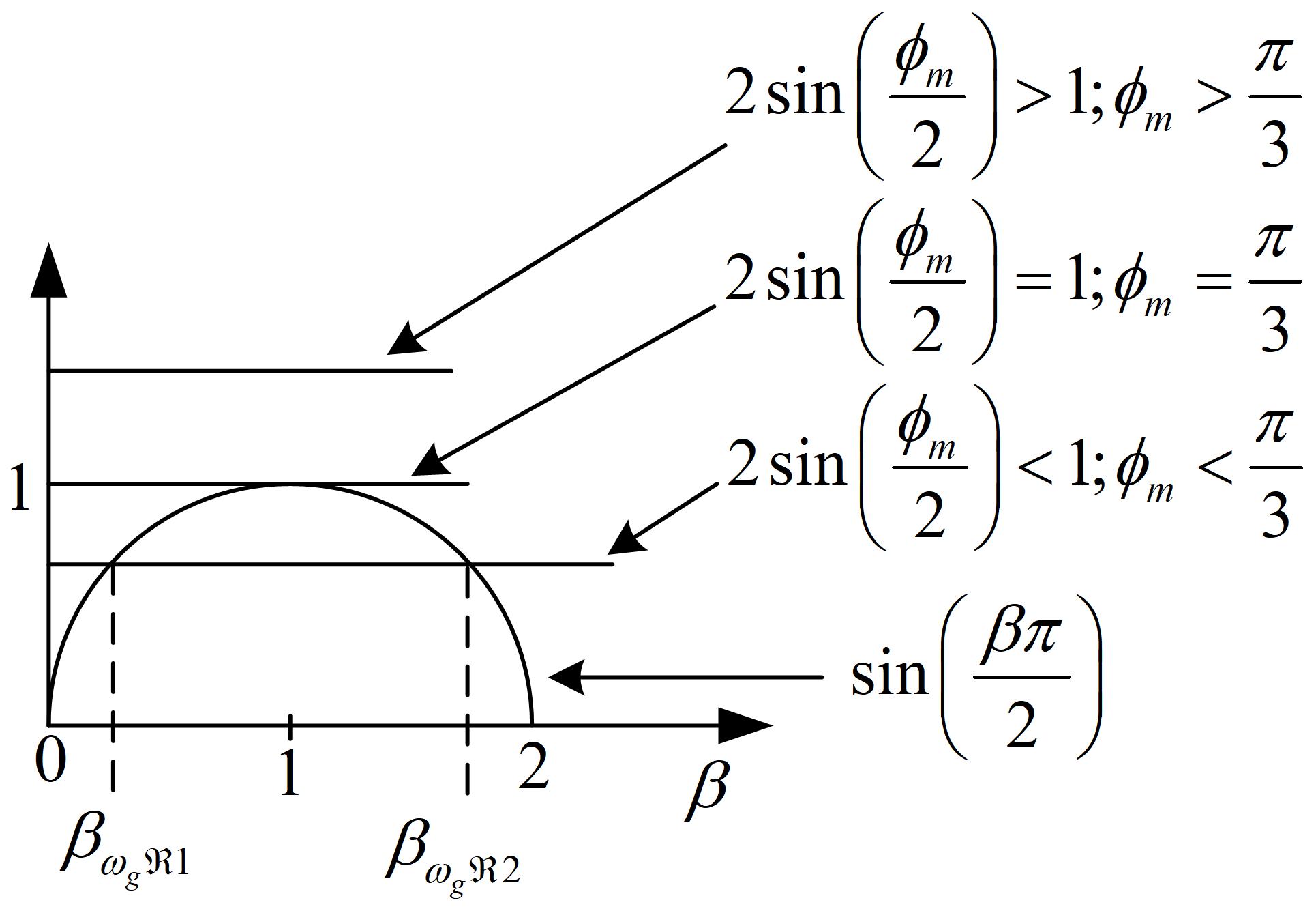
Figure 2: Graphical representation of (36)

In (36), $\beta$ can be considered as a variable and $\phi_{m}$ as an arbitrary constant given by design specification. Plotting LHS and RHS of (36) in Fig.2, two cutoff points of $\beta$ arise, namely $\beta_{{\omega_{g}}\Re 1}$ and $\beta_{{\omega_{g}}\Re 2}$ when $\phi_{m}\in(0,\pi/3)$. At $\phi_{m}=\pi/3$, ${\beta_{{\omega_{g}}\Re 1}}={\beta_{{\omega_{g}}\Re 2}}=1$ and for $\phi_{m}\in[\pi/3,\pi)$, we have $\beta\in(0,2)$. Therefore, if $\phi_{m}\in(0,\pi/3)$, $\beta\in(0,{\beta_{{\omega_{g}}\Re 1}})\cup({\beta_{{\omega_{g}}\Re 2}},2)$ . The boundary values ${\beta_{{\omega_{g}}\Re 1}}$ and ${\beta_{{\omega_{g}}\Re 2}}$ can be found by equating LHS and RHS in (36). i.e

$$\sin\left({\frac{{\beta\pi}}{2}}\right)=2\sin\left({\frac{{{\phi_{m}}}}{2}}\right)$$ (37)

The function $\arcsin$ is defined for the fundamental period $[-\pi/2,\pi/2]$, i.e, if $y\,\in\,[-1,1]$ then $x={\arcsin}\left(y\right)$ implies $x\in[-\pi/2,\pi/2]$. In the present context, in (37), if the argument is in LHS, for $\beta\in(0,1]$ we have $\beta\pi/2\in(0,\pi/2]$ which lies in the fundamental period. Therefore taking inverse will give the correct solution. Hence, if $\beta\in(0,1]$, (37) can be evaluated by directly taking $\arcsin$, and we get

$${\beta_{{\omega_{g}}\Re 1}}=\frac{2}{\pi}{\sin^{-1}}\left({2\sin\left({\frac{{{\phi_{m}}}}{2}}\right)}\right)$$ (38)

However, in (37), for $\beta\in(1,2)$, we have $\beta\pi/2\in(\pi/2,\pi)$, which lies outside of the fundamental period. Therefore, taking $\arcsin$ directly the solution will lie in $[-\pi/2,\pi/2]$, which is incorrect. In such cases, the solution can be corrected by shifting the origin of inverse function in the appropriate domain of the argument. Therefore, for $\beta\in(1,2)$, the origin of the $\arcsin$ need to be shifted as below

$$\frac{{\beta\pi}}{2}-\pi=-\arcsin\left({2\sin\left({\frac{{{\phi_{m}}}}{2}}\right)}\right)$$ (39)

which gives

$${\beta_{{\omega_{g}}\Re 2}}=\frac{2}{\pi}\left({\pi-{{\sin}^{-1}}\left({2\sin\left({\frac{{{\phi_{m}}}}{2}}\right)}\right)}\right)$$ (40)

Next we find $\beta$ so that $\omega_{g}>0$. The expression for $\omega_{g}$ is given in (31). For better understanding, let us denote $\Omega=\cos^{-1}\left({\frac{c_{1}}{r_{1}}}\right)$. Then using (26), we have

$$\Omega=\cos^{-1}\left({\frac{c_{1}}{r_{1}}}\right)=\cos^{-1}\left({\frac{{\sin\left({\frac{{\beta\pi}}{2}}\right)}}{{2\sin\left({\frac{{{\phi_{m}}}}{2}}\right)}}}\right)$$ (41)

Also denoting $\beta\pi/2+\phi_{m}/2=\eta$ in (28), we can write

$$\alpha_{1}=\left\{{\begin{array}[]{*{20}{c}}{-\eta}&{\eta\in{\color[rgb]{0,0,0}\left({0,\frac{\pi}{2}}\right)}}\\ {\pi-\eta}&{\eta\in\left({\frac{\pi}{2},\frac{{3\pi}}{2}}\right)}\end{array}}\right.$$ (42)

With the new notations, the expression of $\omega_{g}$ in (31) becomes,

$${\omega_{g}}=\frac{1}{\theta}\left({-\Omega+{\alpha_{1}}}\right)$$ (43)

In accordance with the controller design, $\phi_{m}\in(0,\pi)$ and $\beta\in(0,2)$. From (26), with arbitrary $\phi_{m}\in(0,\pi)$, we have $c_{1}/r_{1}\in(0,1/\left({2\sin\left({{\phi_{m}}/2}\right)}\right)]$ for both $\beta\in(0,1]$ and $\beta\in(1,2)$. Hence, it can be noted that $c_{1}/r_{1}>0\,\forall\,\beta\in(0,2)$. On the other hand, to have real solution for $\omega_{g}$, we need $\left|c_{1}/r_{1}\right|\leq 1$. Therefore the common admissible range of $c_{1}/r_{1}$ is $(0,1]$. Therefore, $\Omega\in(0,\pi/2]$ from (41).

From (43), for $\omega_{g}>0$ we need $\Omega<\alpha_{1}$. However, it is already shown in previous paragraph that $\Omega\in(0,\pi/2]$. Whereas from (42), $\eta\in(0,3\pi/2)$.

To find ${{\rm B}_{{\omega_{g}}+}}=\left\{{\beta:{\omega_{g}}>0}\right\}$, following three cases need to be considered:

1. $\Omega\in(0,\pi/2]$ and $\eta\in{\color[rgb]{0,0,0}(0,\pi/2)}$ $\Rightarrow{\alpha_{1}}\in\left({-\pi/2,0}\right)$

2. $\Omega\in(0,\pi/2]$ and $\eta\in(\pi/2,\pi]$ $\Rightarrow{\alpha_{1}}\in\left[{0,\pi/2}\right)$

3. $\Omega\in(0,\pi/2]$ and $\eta\in(\pi,3\pi/2)$ $\Rightarrow{\alpha_{1}}\in\left({-\pi/2,0}\right)$

It is clear that cases $(i)$ and $(iii)$ will lead to negative $\omega_{g}$ as $\Omega>\alpha_{1}$ in the entire range of $\Omega$ and $\alpha_{1}$. Hence they are not considered in further analysis.

Lemma 2.4.1 (Existence of solution in $case-ii$)

The solution set $\beta_{{\omega_{g}}+}$ exists only when $\Omega\in(0,\pi/2]$ and $\eta\in(\pi/2,\pi]$.

Proof 2.4.2

From (42), for $\eta\in(\pi/2,\pi]$, we get $\alpha_{1}\in[0,\pi/2)$. Therefore, for $\omega_{g}>0$,

$${\cos^{-1}}\left({\frac{{\sin\left({\frac{{\beta\pi}}{2}}\right)}}{{2\sin\left({\frac{{{\phi_{m}}}}{2}}\right)}}}\right)<\pi-\eta$$ (44)

Above equation can be solved by taking $\cos$ in both side while considering LHS and RHS as arguments. In (44), LHS and RHS both are in $(0,\pi/2)$ and in this range $\cos$ is decreasing function. So taking $\cos$ both side, the inequality is reversed and we get

$$\frac{{\sin\left({\frac{{\beta\pi}}{2}}\right)}}{{2\sin\left({\frac{{{\phi_{m}}}}{2}}\right)}}>\cos\left({\pi-\eta}\right)$$ (45)

Since, $\cos(\pi-x)=-\cos(x)\,;\,x\in(\pi/2,\pi)$, therefore, simplifying (45) and replacing $\eta={\frac{{\beta\pi}}{2}+\frac{{{\phi_{m}}}}{2}}$, we get

$$\frac{{\sin\left({\frac{{\beta\pi}}{2}}\right)}}{{2\sin\left({\frac{{{\phi_{m}}}}{2}}\right)}}>-\cos\left({\frac{{\beta\pi}}{2}+\frac{{{\phi_{m}}}}{2}}\right)$$ (46)

Expanding the RHS and multiplying both side of the inequality by ${2\sin\left({\frac{{{\phi_{m}}}}{2}}\right)}$, we have

$$\sin\left({\frac{{\beta\pi}}{2}}\right)>-\sin\left({{\phi_{m}}}\right)\cos\left({\frac{{\beta\pi}}{2}}\right)+2{\sin^{2}}\left({\frac{{{\phi_{m}}}}{2}}\right)\sin\left({\frac{{\beta\pi}}{2}}\right)$$ (47)

Further, (47) can be simplified by dividing by $\cos(\beta\pi/2)$. However, for $\beta\in(0,1]$, $\cos(\beta\pi/2)\geq 0$. Therefore the inequality sign will not be affected. However, for $\beta\in(1,2)$, $\cos(\beta\pi/2)<0$, and the inequality sign will be reversed. So further classification can be done based on the range of $\beta$.

Case-ii(a): $\beta\in(0,1]$ :
Dividing both side of (47) by $\cos(\beta\pi/2)$ and simplifying, we get

$$\tan\left({\frac{{\beta\pi}}{2}}\right)\left({1-2{{\sin}^{2}}\left({\frac{{{\phi_{m}}}}{2}}\right)}\right)>-\sin\left({{\phi_{m}}}\right)$$ (48)

The plot for $1-2{\sin^{2}}\left({{\phi_{m}}/2}\right)$ is given in Fig.3(a), which is positive when $\phi_{m}\in(0,\pi/2]$ and negative when $\phi_{m}\in(\pi/2,\pi)$. Therefore, $case-ii(a)$ can be further divided as follows.

$Case-ii(a_{1})$, ($\beta\in(0,1]$ and $\phi_{m}\in(0,\pi/2]$): In this case, $1-2{\sin^{2}}\left({{\phi_{m}}/2}\right)$ is positive. Dividing both side of (48) by $1-2{\sin^{2}}\left({{\phi_{m}}/2}\right)$, the inequality sign will remain same. Therefore, we have

$$\tan\left({\frac{{\beta\pi}}{2}}\right)>\frac{{-\sin\left({{\phi_{m}}}\right)}}{{1-2{{\sin}^{2}}\left({\frac{{{\phi_{m}}}}{2}}\right)}}$$ (49)

In (49), LHS and RHS are both functions with range ($-\infty$,$\infty$). From fundamentals of inverse trigonometry we know that when $y=\arctan(x);x\in(-\infty,\infty)$ then $y\in[-\pi/2,\pi/2]$. Since $\arctan$ is increasing function in the fundamental period, therefore, the inequality sign in (49) will remain same on taking $\arctan$ on both side. Therefore, taking $\arctan$ in (49) and evaluating for $\beta$, we get

$$\beta>\frac{2}{\pi}\left({{{\tan}^{-1}}\left({\frac{{-\sin\left({{\phi_{m}}}\right)}}{{1-2{{\sin}^{2}}\left({\frac{{{\phi_{m}}}}{2}}\right)}}}\right)}\right)={\beta_{y1}}(say)$$ (50)

Then, we get the solution set ${{\rm{B}}_{y11}}=\left\{{\beta\in\left({0,1}\right]:\beta>{\beta_{y1}},{\phi_{m}}\in\left({0,\pi/2}\right],{\omega_{g}}>0}\right\}$.

Case-ii$(a_{2})$, ($\beta\in(0,1)$ and $\phi_{m}\in(\pi/2,\pi)$): In this case $1-2{\sin^{2}}\left({{\phi_{m}}/2}\right)$ is negative. Therefore, dividing both side by $1-2{\sin^{2}}\left({{\phi_{m}}/2}\right)$ in (48), the inequality sign will get reverse and we have,

$$\tan\left({\frac{{\beta\pi}}{2}}\right)<\frac{{-\sin\left({{\phi_{m}}}\right)}}{{1-2{{\sin}^{2}}\left({\frac{{{\phi_{m}}}}{2}}\right)}}$$ (51)

In the similar fashion as in $case-ii(a_{1})$, LHS and RHS in (51) are functions with range in $(-\infty,\infty)$. Taking $\arctan$ on both side does not affect the inequality sign in this case. Evaluating for $\beta$, we have

$$\beta<\frac{2}{\pi}\left({{{\tan}^{-1}}\left({\frac{{-\sin\left({{\phi_{m}}}\right)}}{{1-2{{\sin}^{2}}\left({\frac{{{\phi_{m}}}}{2}}\right)}}}\right)}\right)={\beta_{y1}}$$ (52)

Therefore, we get the solution set ${\color[rgb]{0,0,0}{{\rm{B}}_{y12}}=\left\{{\beta\in\left({0,1}\right]:\beta<{\beta_{y1}},{\phi_{m}}\in\left({\pi/2,\pi}\right),{\omega_{g}}>0}\right\}}$.

Case-ii(b): $\beta\in(1,2)$ :
In (47), dividing both side by $\cos(\beta\pi/2)$, we get

$$\tan\left({\frac{{\beta\pi}}{2}}\right)<-\sin\left({{\phi_{m}}}\right)+2\tan\left({\frac{{\beta\pi}}{2}}\right){\sin^{2}}\left({\frac{{{\phi_{m}}}}{2}}\right)$$ (53)

Simplifying (53), we get

$$\tan\left({\frac{{\beta\pi}}{2}}\right)\left({1-2{{\sin}^{2}}\left({\frac{{{\phi_{m}}}}{2}}\right)}\right)<-\sin\left({{\phi_{m}}}\right)$$ (54)

Again, from Fig.3(a), $1-2{\sin^{2}}\left({{\phi_{m}}/2}\right)$ is negative for $\phi_{m}\in(0,\pi/2]$ and positive for $\phi_{m}\in(\pi/2,\pi)$. Therefore, $case-ii(b)$ can be further divided into two sub cases according to the range of $\phi_{m}$.

case-ii$(b_{1})$, ($\beta$$\in$(1,2) and $\phi_{m}\in(0,\pi/2]$): In this case, $1-2{\sin^{2}}\left({{\phi_{m}}/2}\right)$ is positive, therefore, dividing both side in (54) by $1-2{\sin^{2}}\left({{\phi_{m}}/2}\right)$, the inequality sign will not be affected. Therefore, we get

$$\tan\left({\frac{{\beta\pi}}{2}}\right)<\frac{{-\sin\left({{\phi_{m}}}\right)}}{{1-2{{\sin}^{2}}\left({\frac{{{\phi_{m}}}}{2}}\right)}}$$ (55)

To evaluate $\beta$ from (55), we need to take $\arctan$ on both side. From fundamental of trigonometry, ${\tan^{-1}}\left({\tan\left(x\right)}\right)=x|x\in(-\pi/2,\pi/2)$. Notice that the argument $\beta\pi/2$ lies in $(\pi/2,\pi)$ for $\beta\in(1,2)$, which is outside the range of fundamental period. In this case the origin needs to be shifted as $\tan\left({\frac{{\beta\pi}}{2}}\right)=\tan\left({\frac{{\beta\pi}}{2}-\pi}\right)$. Therefore, to get correct solution from (55), we need to solve

$$\tan\left({\frac{{\beta\pi}}{2}-\pi}\right)<\frac{{-\sin\left({{\phi_{m}}}\right)}}{{1-2{{\sin}^{2}}\left({\frac{{{\phi_{m}}}}{2}}\right)}}$$ (56)

In (56), for $\beta\in(1,2)$, $\tan(\beta\pi/2-\pi)\in(-\infty,0)$ and $\arctan(-\infty,0)\in(0,\pi/2)$. However, in $(0,\pi/2)$, $\arctan$ is increasing function. Therefore, the inequality sign will remain same on taking $\arctan$ on both side.

Therefore, taking $\arctan$ on both side of (56), we get

$$\frac{{\beta\pi}}{2}-\pi<{\tan^{-1}}\left({\frac{{-\sin\left({{\phi_{m}}}\right)}}{{1-2{{\sin}^{2}}\left({\frac{{{\phi_{m}}}}{2}}\right)}}}\right)$$

Evaluating for $\beta$, we get

$$\beta<\frac{2}{\pi}\left({\pi+{{\tan}^{-1}}\left({\frac{{-\sin\left({{\phi_{m}}}\right)}}{{1-2{{\sin}^{2}}\left({\frac{{{\phi_{m}}}}{2}}\right)}}}\right)}\right)=\beta_{y2}(say)$$ (57)

Then we have the solution set as ${\color[rgb]{0,0,0}{{\rm{B}}_{y21}}=\left\{{\beta\in\left({1,2}\right):\beta<{\beta_{y2}},{\phi_{m}}\in\left({0,\pi/2}\right],{\omega_{g}}>0}\right\}}$.

case-ii$(b_{2})$, ($\beta\in(1,2)$ and $\phi_{m}\in(\pi/2,\pi)$): In this case, $1-2{\sin^{2}}\left({{\phi_{m}}/2}\right)$ is negative. Therefore, dividing both side in (54) by $1-2{\sin^{2}}\left({{\phi_{m}}/2}\right)$ the sign of inequality will get reversed. Hence, we have

$$\tan\left({\frac{{\beta\pi}}{2}}\right)>\frac{{-\sin\left({{\phi_{m}}}\right)}}{{1-2{{\sin}^{2}}\left({\frac{{{\phi_{m}}}}{2}}\right)}}$$ (58)

Again, for $\beta\in(1,2)$, $\beta\pi/2\in(\pi/2,\pi)$ which is outside the range of fundamental period of $\tan(x)$. Therefore, we shift the origin and get

$$\tan\left({\frac{{\beta\pi}}{2}-\pi}\right)>\frac{{-\sin\left({{\phi_{m}}}\right)}}{{1-2{{\sin}^{2}}\left({\frac{{{\phi_{m}}}}{2}}\right)}}$$ (59)

In this range $\arctan$ is increasing function. Thus, we get,

$$\beta>\frac{2}{\pi}\left({\pi+{{\tan}^{-1}}\left({\frac{{-\sin\left({{\phi_{m}}}\right)}}{{1-2{{\sin}^{2}}\left({\frac{{{\phi_{m}}}}{2}}\right)}}}\right)}\right)=\beta_{y2}$$ (60)

Therefore, the solution set is ${\color[rgb]{0,0,0}{{\rm{B}}_{y22}}=\left\{{\beta\in\left({1,2}\right):\beta>{\beta_{y2}},{\phi_{m}}\in\left({\pi/2,\pi}\right),{\omega_{g}}>0}\right\}}$.

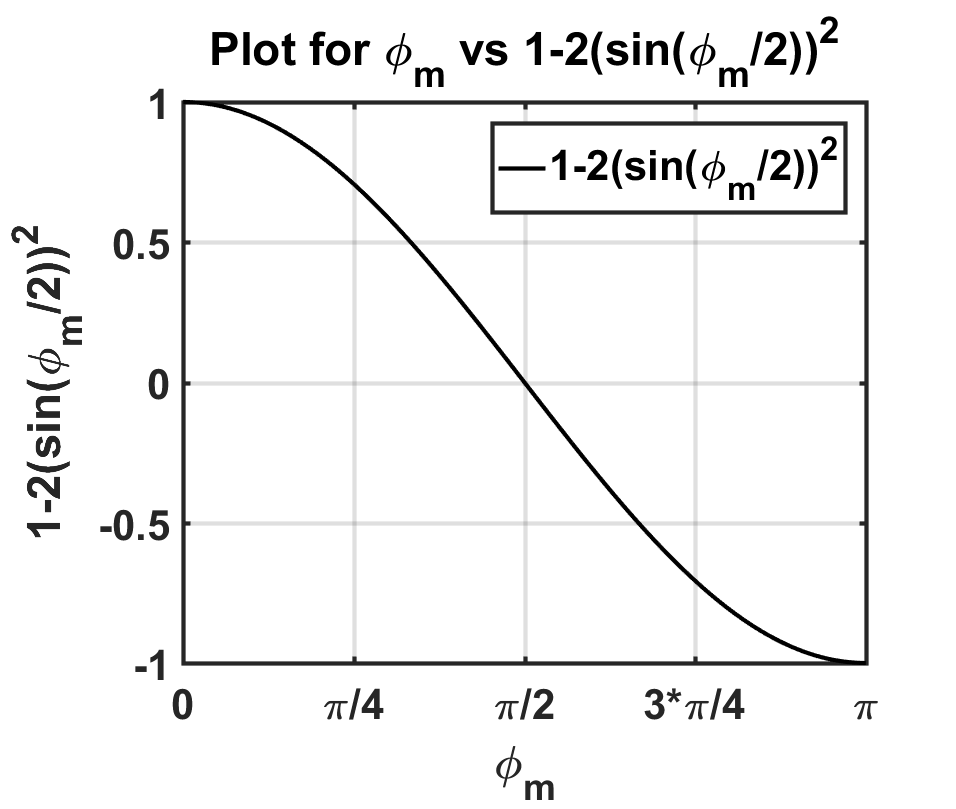
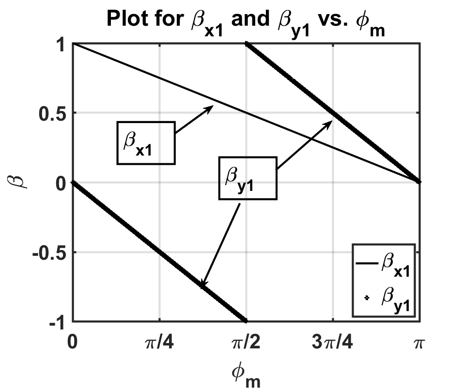
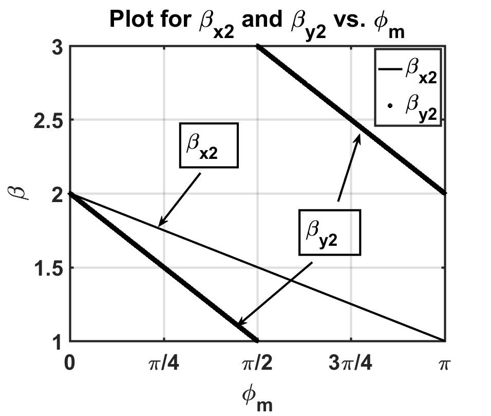
Figure 3: Graphical representation of (a) $\phi_{m}$ vs. $1-2{\sin^{2}}\left({{\phi_{m}}/2}\right)$, (b) $\phi_{m}$ vs. $\beta_{x1}$ and $\phi_{m}$ vs. $\beta_{y1}$, (c) $\phi_{m}$ vs. $\beta_{x2}$ and $\phi_{m}$ vs. $\beta_{y2}$.

The above four cases are summarized in Table-1. From Fig.3(c), we can see that no $\beta\in(1,2)$ for $\phi_{m}\in(\pi/2,\pi)$ exists such that $\beta>\beta_{y2}$. Hence, there is no solution for $case-ii(b_{2})$. From the same figure, it is evident that the other three cases can have solution for $\beta$.

Table 1: Existence of solution such that $\omega_{g}>0$

	${{\phi_{m}}\in\left({0,\pi/2}\right]}$	${{\phi_{m}}\in\left({\pi/2,\pi}\right)}$
${\beta\in\left({0,1}\right]}$	$case-ii(a_{1})$, ${\rm B}_{y11}={\beta>{\beta_{y1}}}$	$case-ii(a_{2})$, ${\rm B}_{y12}={\beta<{\beta_{y1}}}$
${\beta\in\left({1,2}\right)}$	$case-ii(b_{1})$, ${\rm B}_{y21}={\beta<{\beta_{y2}}}$	$case-ii(b_{2})$, ${\rm B}_{y22}={\beta>{\beta_{y2}}}$

Lemma-3 gives the possible solution for ${\rm B}_{{\omega_{g}}+}$ when $\eta\in(\pi/2,\pi]$. Since, $\eta=(\beta\pi/2+\phi_{m}/2)$, this implies $\beta\in((\pi-\phi_{m})/\pi,(2\pi-\phi_{m})/\pi]$. Let a set ${{\rm B}_{x}}=\left\{{\beta:\beta\in\left({{\beta_{{x1}}},{\beta_{x2}}}\right]}\right\}$, where ${\beta_{{x1}}}=((\pi-\phi_{m})/\pi)$ and ${\beta_{{x2}}}=(2\pi-\phi_{m})/\pi$. Therefore, ${\rm B}_{{\omega_{g}}+}$ can be found from intersection of solution set in Lemma-3 and the set ${{\rm B}_{x}}$. Therefore, the task that remains is to find ${\rm B}_{{\omega_{g}}+}$ for each of the valid three cases.
Note: For $\phi_{m}\in(0,\pi)$, $\beta_{x1}\in(0,1)$ and $\beta_{x2}\in(1,2)$.

Theorem 2.4.2 (Finding ${\rm B}_{{\omega_{g}}+}$)

The set ${\rm B}_{{\omega_{g}}+}$ containing solution $\beta$ when $\omega_{g}>0$ is given as ${\color[rgb]{0,0,0}{{\rm B}_{{\omega_{g}}+}}=\left\{{\beta:\beta\in({\beta_{x1}},{\beta_{y2}})}\right\}}$ when $\phi_{m}\in(0,\pi/2]$ and ${\color[rgb]{0,0,0}{{\rm B}_{{\omega_{g}}+}}=\left\{{\beta:\beta\in({\beta_{x1}},{\beta_{y1}})}\right\}}$
when $\phi_{m}\in(\pi/2,\pi)$, where
$\beta_{x_{1}}=(\pi-\phi_{m})/\pi$, ${\beta_{y1}}=\frac{2}{\pi}\left({{{\tan}^{-1}}\left({\frac{{-\sin\left({{\phi_{m}}}\right)}}{{1-2{{\sin}^{2}}\left({\frac{{{\phi_{m}}}}{2}}\right)}}}\right)}\right)$ and $\beta_{y2}=\frac{2}{\pi}\left({\pi+{{\tan}^{-1}}\left({\frac{{-\sin\left({{\phi_{m}}}\right)}}{{1-2{{\sin}^{2}}\left({\frac{{{\phi_{m}}}}{2}}\right)}}}\right)}\right)$ are given in (30), (50) and (57) respectively.

Proof 2.4.3

$Case-ii(a_{1})$, ($\beta\in(0,1]$, $\phi_{m}\in(0,\pi/2]$): ${\rm B}_{{\omega_{g}}+}={\rm B}_{x}\cap{\rm B}_{y11}$ where, ${{\text{B}}_{x}}=\left\{{\beta:\beta\in\left({{\beta_{x1}},{\beta_{x2}}}\right]}\right\}$ and ${{\text{B}}_{y11}}=\left\{{\beta:\beta>{\beta_{y1}}}\right\}$. From Fig.3(a), $\beta_{y1}\in(-1,0)$, whereas $\beta_{x1}\in(0,1)$ and $\beta_{x2}\in(1,2)$. Therefore, in this scenario we have ${\color[rgb]{0,0,0}{{\rm B}_{x}}=\left\{{\beta:\beta\in({\beta_{x1}},1]}\right\}}$ and ${{\rm B}_{y11}}=\left\{{\beta:\beta\in(0,1]}\right\}$. Hence, the intersection of ${\rm B}_{x}$ and ${\rm B}_{y11}$ will be the solution set ${\color[rgb]{0,0,0}{{\rm B}_{{\omega_{g}}+}}=\left\{{\beta:\beta\in({\beta_{x1}},1]:{\phi_{m}}\in(0,\pi/2]}\right\}}$.

$Case-ii(b_{1})$, ($\beta\in(1,2),\phi_{m}\in(0,\pi/2]$): ${\rm B}_{{\omega_{g}}+}={\rm B}_{x}\cap{\rm B}_{y21}$, where, ${{\rm B}_{y21}}=\left\{{\beta:\beta<{\beta_{y2}}}\right\}$. From Fig.3(b), for $\phi_{m}\in(0,\pi/2)$, $\beta_{y2}\in(1,2)$, whereas $\beta_{x2}\in(1,2)$. Therefore, in this scenario we have ${{\rm B}_{x}}=\left\{{\beta:\beta\in(1,{\beta_{x2}})}\right\}$ and ${{\rm B}_{y21}}=\left\{{\beta:\beta\in(1,{\beta_{y2}})}\right\}$. Therefore, ${{\rm B}_{{\omega_{g}}+}}={\rm B}_{x}\cap{\rm B}_{y21}=\left\{{\beta:\beta\in\left({1,\min\left({{\beta_{x2}},{\beta_{y2}}}\right)}\right)}\right\}$. From, Fig.3(b), for $\phi_{m}\in(0,\pi/2)$, $\beta_{y2}<\beta_{x2}$. Therefore, ${{\rm B}_{{\omega_{g}}+}}=\left\{{\beta:\beta\in\left({1,{\beta_{y2}}}\right)}\right\}$.

Combining $Case-ii(a_{1})$ and $Case-ii(b_{1})$, for $\phi_{m}\in(0,\pi/2]$, ${{\rm B}_{{\omega_{g}}+}}=\left\{{\beta:\beta\in\left({{\beta_{x1}},1}\right]\cup\left({1,{\beta_{y2}}}\right)}\right\}=\{\beta:\beta\in\left({{\beta_{x1}},{\beta_{y2}}}\right)\}$.

$Case-ii(a_{2})$, ($\beta\in(0,1),\phi_{m}\in(\pi/2,\pi)$): ${\rm B}_{{\omega_{g}}+}={\rm B}_{x}\cap{\rm B}_{y12}$, where, ${{\rm B}_{y12}}=\left\{{\beta:\beta<{\beta_{y1}}}\right\}$. From Fig.3(a), for $\phi_{m}\in(0,\pi/2)$, $\beta_{y1}\in(0,1)$, whereas $\beta_{x1}\in(0,1)$ and $\beta_{x2}\in(1,2)$. Therefore, in this scenario we have ${{\rm B}_{x}}=\left\{{\beta:\beta\in({\beta_{x1}},1]}\right\}$ and ${{\text{B}}_{y12}}=\left\{{\beta:\beta\in\left({0,{\beta_{y1}}}\right)}\right\}$. For existence of solution, we must have $\beta_{x1}<\beta_{y1}$. From Fig.3(a), for $\phi_{m}\in(\pi/2,\pi)$, $\beta_{x1}<\beta_{y1}$. Therefore, ${{\rm B}_{{\omega_{g}}+}}=\left\{{\beta:\beta\in\left({{\beta_{x1}},{\beta_{y1}}}\right)}\right\}$ for $\phi_{m}\in(\pi/2,\pi)$.

Now $\beta_{{\omega_{g}}}$ can be found by combining Theorem-2 and 3.

Theorem 2.4.3 (Finding ${\rm B}_{{\omega_{g}}}$)

The set ${\rm B}_{{\omega_{g}}}$ such that $\omega_{g}\in\Re^{+}$ is given as:
(a) ${{\rm B}_{{\omega_{g}}}}=\left\{{\beta:\beta\in\left({{\beta_{{\omega_{g}}\Re 2}},{\beta_{y2}}}\right)}\right\}$ when $\phi_{m}\in(0,0.9273]$,
(b) ${{\rm B}_{{\omega_{g}}}}=\left\{{\beta:\beta\in\left({{\beta_{x1}},{\beta_{{\omega_{g}}\Re 1}}}\right)\cup\left({{\beta_{{\omega_{g}}\Re 2}},{\beta_{y2}}}\right)}\right\}$ when $\phi_{m}\in(0.9273,\pi/3)$,
(c) ${{\rm B}_{{\omega_{g}}}}=\left\{{\beta:\beta\in\left({{\beta_{x1}},{\beta_{y2}}}\right)}\right\}$ when $\phi_{m}\in[\pi/3,\pi/2]$, and
(d) ${{\rm B}_{{\omega_{g}}}}=\left\{{\beta:\beta\in\left({{\beta_{x1}},{\beta_{y1}}}\right)}\right\}$ when $\phi_{m}\in(\pi/2,\pi)$.

Proof 2.4.4

From Theorem-2, ${{\rm{B}}_{{\omega_{g}}\Re}}=\{\beta:\beta\in(0,{\beta_{{\omega_{g}}\Re 1}})\cup({\beta_{{\omega_{g}}\Re 2}},2)\}$ for $\phi_{m}\in(0,\pi/3)$, whereas, ${{\rm{B}}_{{\omega_{g}}\Re}}=\{\beta:\beta\in(0,2)\}$ for $\phi_{m}\in[\pi/3,\pi)$. However, from Theorem-3, ${{\rm{B}}_{{\omega_{g}}+}}=\{\beta:\beta\in({\beta_{x1}},{\beta_{y2}})\}$ if $\phi_{m}\in(0,\pi/2]$, whereas ${{\rm{B}}_{{\omega_{g}}+}}=\{\beta:\beta\in({\beta_{x1}},{\beta_{y1}})\}$ if $\phi_{m}\in(\pi/2,\pi)$. Therefore, combining Theorem 2 and 3, following three cases are possible.

Case-I, $\phi_{m}\in(0,\pi/3)$: In this case, ${{\rm{B}}_{{\omega_{g}}\Re}}=\{\beta:\beta\in(0,{\beta_{{\omega_{g}}\Re 1}})\cup({\beta_{{\omega_{g}}\Re 2}},2)\}$ and ${{\rm{B}}_{{\omega_{g}}+}}=\{\beta:\beta\in({\beta_{x1}},{\beta_{y1}})\}$. For existence of solution in $\beta\in(0,1)$, we must have $\beta_{x1}<\beta_{{\omega_{g}}\Re 1}$ and for existence of solution in $\beta(1,2)$, $\beta_{{\omega_{g}}\Re 2}<\beta_{y2}$ is needed.

In Fig.4(a), $\beta_{x1}-\beta_{{\omega_{g}}\Re 1}$ plot and in Fig.4(b), $\beta_{y2}-\beta_{{\omega_{g}}\Re 2}$ plot with respect to $\phi_{m}\in(0,\pi/3)$ is given. It can be seen that $\beta_{x1}<\beta_{{\omega_{g}}\Re 1}$ is satisfied for $\phi_{m}\in(0.9273,\pi/3)$, and if $\phi_{m}\in(0,0.9273]$, there is no $\beta\in(0,1)$ such that $\omega_{g}>0$. However, from Fig.4(b), $\beta_{{\omega_{g}}\Re 2}<\beta_{y2}\forall\phi_{m}\in(0,\pi/3)$. Therefore, ${{\rm{B}}_{{\omega_{g}}}}=\{\beta:\beta\in({\beta_{{\omega_{g}}\Re 2}},{\beta_{y2}})\}$ in this case.

This concludes that if $\phi_{m}\in(0,0.9273]$, then ${{\rm B}_{{\omega_{g}}}}=\left\{{\beta:\beta\in\left({{\beta_{{\omega_{g}}\Re 2}},{\beta_{y2}}}\right)}\right\}$ and if $\phi_{m}\in(0.9273,\pi/3)$, then ${{\rm B}_{{\omega_{g}}}}=\left\{{\beta:\beta\in\left({{\beta_{x1}},{\beta_{{\omega_{g}}\Re 1}}}\right)\cup\left({{\beta_{{\omega_{g}}\Re 2}},{\beta_{y2}}}\right)}\right\}$.

Part (a) and (b) of the theorem is hence proved.

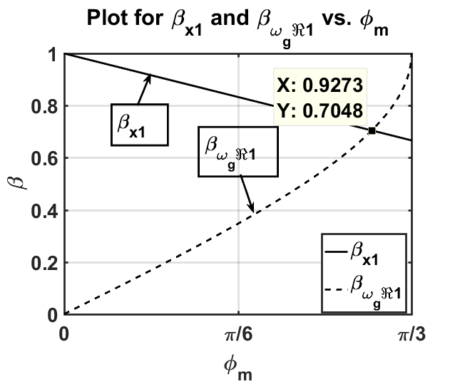
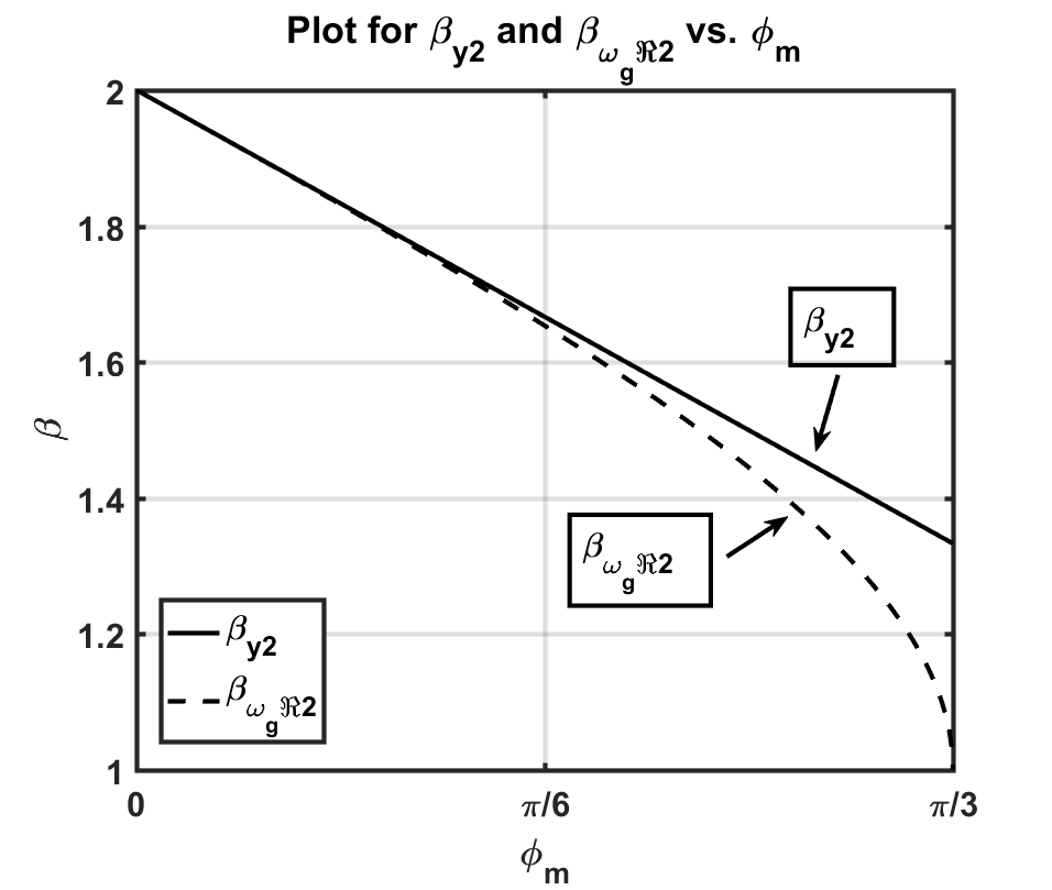
Figure 4: Graphical representation of (a) $\phi_{m}$ vs. $\beta_{x1}$ and $\phi_{m}$ vs. $\beta_{{\omega_{g}}\Re 1}$ (b) $\phi_{m}$ vs. $\beta_{y2}$ and $\phi_{m}$ vs. $\beta_{{\omega_{g}}\Re 2}$

Case-II, $\phi_{m}\in[\pi/3,\pi/2]$: In this case, ${{\rm B}_{{\omega_{g}}\Re}}=\left\{{\beta:\beta\in\left({0,2}\right)}\right\}$ and ${\beta_{{\omega_{g}}+}}=\left\{{\beta:\beta\in({\beta_{x1}},{\beta_{y2}})}\right\}$. Since, ${{\rm B}_{{\omega_{g}}}}={{\rm B}_{{\omega_{g}}\Re}}\cap{{\rm B}_{{\omega_{g}}+}}$, therefore, ${{\rm{B}}_{{\omega_{g}}}}={{\rm{B}}_{{\omega_{g}}+}}=\left\{{\beta:\beta\in\left({{\beta_{x1}},{\beta_{y2}}}\right)}\right\}$. This proves part (c) of the theorem.

Case-III, $\phi_{m}\in(\pi/2,\pi)$: In this case, ${{\rm B}_{{\omega_{g}}\Re}}=\left\{{\beta:\beta\in\left({0,2}\right)}\right\}$ and ${{\rm{B}}_{{\omega_{g+}}}}=\left\{{\beta:\beta\in\left({{\beta_{x1}},{\beta_{y1}}}\right)}\right\}$. Therefore, ${{\rm{B}}_{{\omega_{g}}}}={{\rm{B}}_{{\omega_{g}}+}}=\left\{{\beta:\beta\in\left({{\beta_{x1}},{\beta_{y1}}}\right)}\right\}$. This proves part (d) of the theorem.

2.5 Finding $\omega_{p}\in\Xi_{b}$:

Eliminating $\lambda$ in (17) and (18), we get

$$\tan\left({\frac{{\beta\pi}}{2}}\right)=\frac{{{A_{m}}\sin\left({\theta{\omega_{p}}}\right)-\sin\left({\theta{\omega_{p}}}\right)}}{{\cos\left({\theta{\omega_{p}}}\right)-{A_{m}}\cos\left({\theta{\omega_{p}}}\right)-1}}$$ (61)

In (61), there are four variables $\omega_{g}$, $\beta,\theta$ and $A_{m}$. Here $\theta$ is the delay of the process and known, $A_{m}$ is the desired gain margin specification and $\beta$ and $\omega_{p}$ are unknown variables that need to be evaluated. Simplifying (61), we have

$$\begin{array}[]{c}\tan\left({\frac{{\beta\pi}}{2}}\right)\left({1-A_{m}}\right)\cos\left({\theta{\omega_{p}}}\right)-\left({A_{m}-1}\right)\sin\left({\theta{\omega_{p}}}\right)=\tan\left({\frac{{\beta\pi}}{2}}\right)\end{array}$$

$$\text{or,}\qquad\tan\left({\frac{{\beta\pi}}{2}}\right)\cos\left({\theta{\omega_{p}}}\right)+\sin\left({\theta{\omega_{p}}}\right)=\frac{{\tan\left({\frac{{\beta\pi}}{2}}\right)}}{{1-{A_{m}}}}$$ (62)

which can be further simplified as

$${a_{2}}\cos\left({\theta{\omega_{p}}}\right)+{b_{2}}\sin\left({\theta{\omega_{p}}}\right)={c_{2}}$$ (63)

$$\text{where}\qquad\begin{array}[]{c}a_{2}=\tan\left({\frac{{\beta\pi}}{2}}\right);\,b_{2}=1;\,c_{2}=\frac{{\tan\left({\frac{{\beta\pi}}{2}}\right)}}{{1-{A_{m}}}}\end{array}$$ (65)

Now, let $a_{2}=r_{2}\cos\left(\alpha_{2}\right)$ and $b_{2}=r_{2}\sin\left(\alpha_{2}\right)$, where ${r_{2}}=\sqrt{a_{2}^{2}+b_{2}^{2}}$ and ${\alpha_{2}}={\tan^{-1}}\left({\frac{{{b_{2}}}}{{{a_{2}}}}}\right)$. Using trigonometric identity, $\cos(x)\cos(y)+\sin(x)\sin(y)=\cos(x-y)$. Assuming $\theta\omega_{p}=x$ and $\alpha_{2}=y$, (63) becomes

$$\qquad\cos\left({\theta{\omega_{p}}-{\alpha_{2}}}\right)=\frac{c_{2}}{r_{2}}$$ (66)

Lemma 2.5.1 (Simplification for $c_{2}/r_{2}$)

If $a_{2}$, $b_{2}$ and $c_{2}$ are as given in (65), then $c_{2}/r_{2}$ can be given as

$$\frac{{{c_{2}}}}{{{r_{2}}}}=-\frac{{\sin\left({\frac{{\beta\pi}}{2}}\right)}}{{{A_{m}}-1}}$$ (67)

Proof 2.5.1

With $a_{2}$ and $b_{2}$ from (65), we get ${r_{2}}=\sec\left({\frac{{\beta\pi}}{2}}\right)$. Therefore, we have

$$\frac{{{c_{2}}}}{{{r_{2}}}}=-\frac{{\sin\left({\frac{{\beta\pi}}{2}}\right)}}{{{A_{m}}-1}}$$ (68)

Note that $c_{2}/r_{2}$ in (67), is a negative quantity because $\beta\in(0,2)$ and $A_{m}>1$.

Lemma 2.5.2 (Simplification of $\alpha_{2}$)

$\alpha_{2}$ in (66) can be simplified as

$${\alpha_{2}}=\frac{\pi}{2}-\frac{{\beta\pi}}{2}$$ (69)

where ${\alpha_{2}}={\tan^{-1}}\left({\frac{{{b_{2}}}}{{{a_{2}}}}}\right)$.

Proof 2.5.2

We have $\alpha_{2}=\tan^{-1}(b_{2}/a_{2})$. Substituting $a_{2}$ and $b_{2}$ from (65), we get

$${\alpha_{2}}={\tan^{-1}}\left({\frac{1}{{\tan\frac{{\beta\pi}}{2}}}}\right)={\tan^{-1}}\left({\cot\frac{{\beta\pi}}{2}}\right)$$ (70)

Using trigonometric identity, $\cot(x)=\tan(\pi/2-x)\forall x\in\Re$, we get

$${\alpha_{2}}={\tan^{-1}}\left({\tan\left({\frac{\pi}{2}-\frac{{\beta\pi}}{2}}\right)}\right)$$

In (70), for $\beta\in(0,2)$, the argument lies in $(-\pi/2,\pi/2)$. Now, $\tan^{-1}(\tan(x))=x$ when $x\in[-\pi/2,\pi/2]$. Therefore,

$${\alpha_{2}}=\frac{\pi}{2}-\frac{{\beta\pi}}{2}$$ (71)

Theorem 2.5.1 (Solution of $\omega_{p}$)

If $\beta\in(0,2)$ and $A_{m}>1$, then

$${\omega_{p}}=\frac{1}{\theta}\left({\pi-{{\cos}^{-1}}\left({\frac{{\sin\left({\frac{{\beta\pi}}{2}}\right)}}{{{A_{m}}-1}}}\right)+\frac{\pi}{2}-\frac{{\beta\pi}}{2}}\right)$$ (72)

Proof 2.5.3

The expression of $\omega_{p}$ can be found from (66) as

$${\omega_{p}}=\frac{1}{\theta}\left({{{\cos}^{-1}}\left({\frac{{{c_{2}}}}{r_{2}}}\right)+{\alpha_{2}}}\right)$$ (73)

Let us assume ${\cos^{-1}}(c_{2}/r_{2})=\zeta$ and from (67), $c_{2}/r_{2}<0$. Therefore, using inverse trigonometric property, $\cos^{-1}(-x)=\pi-\cos^{-1}(x);\,x>0$, we have

$$\zeta=\pi-{\cos^{-1}}\left({\frac{{\sin\left({\frac{{\beta\pi}}{2}}\right)}}{{{A_{m}}-1}}}\right)$$ (74)

From (73), (74) and (69) we have

$${\omega_{p}}=\frac{1}{\theta}\left({\zeta+\alpha_{2}}\right)$$ (75)

Substituting $\zeta$ from (74) and $\alpha_{2}$ from (69), we get

$${\omega_{p}}=\frac{1}{\theta}\left({\pi-{{\cos}^{-1}}\left({\frac{{\sin\left({\frac{{\beta\pi}}{2}}\right)}}{{{A_{m}}-1}}}\right)+\frac{\pi}{2}-\frac{{\beta\pi}}{2}}\right)$$ (76)

Remark 1

For $A_{m}=1$, $c_{2}/r_{2}\to\infty$ . Therefore, $A_{m}=1$ cannot be chosen as controller design specification. Whereas, $A_{m}<1$ signifies an unstable closed loop system, thus irrelevant from control point of view.

2.6 Finding $\beta_{\omega_{p}}$ from set $\Xi_{b}$:

For any practical control system, we have $\omega_{p}\in\Re^{+}$. Let ${\rm B}_{{\omega_{p}}}$ is the set of those $\beta$ which satisfies some given $\omega_{p}$. Therefore, it is justified to write ${{\rm B}_{{\omega_{p}}}}=\left\{{\beta:{\omega_{p}}\in{\Re^{+}}}\right\}$.

In (72), $\omega_{p}$ is function of $\theta$, $\beta$ and $A_{m}$, where $\theta$ is the process delay, $A_{m}$ is the desired gain margin and $\beta\in(0,2)$. The solution can be found in two steps. First, find ${{\rm B}_{{\omega_{p}}\Re}}=\left\{{\beta:{\omega_{p}}\in\Re}\right\}$ and second, find ${{\rm B}_{{\omega_{p}}+}}=\left\{{\beta:{\omega_{p}}>0}\right\}$. Then, ${{\rm B}_{{\omega_{p}}}}={{\rm B}_{{\omega_{p}}\Re}}\cap{{\rm B}_{{\omega_{p}}+}}$.

Theorem 2.6.1 (Condition for $\omega_{p}\in\Re$)

If $\omega_{p}\in\Re$ is as given in (73), where $c_{2}/r_{2}$ is as given in (67), then for $\beta\in(0,2)$ and $A_{m}\geq 2$, ${{\rm B}_{{\omega_{p}}+}}=\left\{{\beta\in(0,2):{\omega_{p}}>0}\right\}$.

Proof 2.6.1

For $\omega_{p}\in\Re$, $\left|c_{2}/r_{2}\right|\leq 1$. Hence, (67) can be written as

$$\left|\frac{\sin\left(\frac{\beta\pi}{2}\right)}{A_{m}-1}\right|\leq 1$$ (77)

For $\beta\in(0,2)$, $\sin\left(\beta\pi/2\right)>0$ and also for $A_{m}\geq 2$, $A_{m}-1>0$. Therefore, the modulus sign can be eliminated in in left hand side in (77), thus, we have

$$\sin\left({\frac{{\beta\pi}}{2}}\right)\leq{{A_{m}}-1}$$ (78)

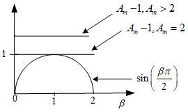
Figure 5: Graphical representation of (78)

In Fig.5, LHS and RHS of (78) is plotted for $\beta\in(0,2)$ and $A_{m}\geq 2$ respectively. From the figure, it is clear that the condition in (78), i.e., for $A_{m}\geq 2$, $\omega_{p}\in\Re\,\forall\,\beta\in(0,2)$.

Theorem 2.6.2 (Condition for $\omega_{p}>0$ )

If $\beta\in(0,2)$ and $A_{m}\geq 1$, then ${{\rm B}_{{\omega_{p}}+}}=\left\{{\beta\in(0,2):{\omega_{p}}>0}\right\}$.

Proof 2.6.2

Referring to (75), for $\omega_{p}>0$, we need

$$\zeta>-\alpha_{2}$$ (79)

where $\zeta$ is given in (74) and $\alpha_{2}$ is given in (71). Substituting $\zeta$ and $\alpha_{2}$, (79) can be written as

$$\pi-{\cos^{-1}}\left({\frac{{\sin\left({\frac{{\beta\pi}}{2}}\right)}}{{{A_{m}}-1}}}\right)>-\frac{\pi}{2}+\frac{{\beta\pi}}{2}$$ (80)

In (80), let us denote, $\gamma_{1}=\pi-{\cos^{-1}}\left({\frac{{\sin\left({\frac{{\beta\pi}}{2}}\right)}}{{{A_{m}}-1}}}\right)$ and $\gamma_{2}=-\frac{\pi}{2}+\frac{{\beta\pi}}{2}$. Therefore, we need to prove that $\gamma_{1}>\gamma_{2}$ for $A_{m}\geq 2$ and $\beta\in(0,2)$.

For $\beta\in(0,1]$, $\frac{{\sin\left({\beta\pi/2}\right)}}{{{A_{m}}-1}}\in\left({0,\frac{1}{{{A_{m}}-1}}}\right]$ and for $\beta(1,2)$, $\frac{{\sin\left({\beta\pi/2}\right)}}{{{A_{m}}-1}}\in\left({0,\frac{1}{{{A_{m}}-1}}}\right)$. However, ${\frac{1}{{{A_{m}}-1}}}\in(0,1]$ for $A_{m}\geq 2$. Therefore, $\left({\frac{{\sin\left({{{\beta\pi}}/{2}}\right)}}{{{A_{m}}-1}}}\right)\in(0,1]$ for all $\beta\in(0,2)$ and $A_{m}\geq 2$. Hence, $\cos^{-1}\left({\frac{{\sin\left({{{\beta\pi}}/{2}}\right)}}{{{A_{m}}-1}}}\right)\in[0,\pi/2)$ for $\beta\in(0,2)$ and $A_{m}\geq 2$, which results $\gamma_{1}\in(\pi/2,\pi]$.

Similarly, for $\beta\in(0,2)$, $\gamma_{2}\in(-\pi/2,\pi/2)$. Therefore, $\gamma_{1}>\gamma_{2}$ for all $\beta\in(0,2)$ and $A_{m}\geq 2$. Hence, it concludes that $\omega_{p}>0\,\forall\,\{\beta\in(0,2),\,A_{m}\geq 2\}$.

From Theorem 6 and 7, we have ${{\rm B}_{{\omega_{p}}\Re}}=\left\{{\beta\in\left({0,2}\right):{\omega_{p}}\in\Re}\right\}$ and
${{\rm B}_{{\omega_{p}}+}}=\left\{{\beta\in\left({0,2}\right):{\omega_{p}}>0}\right\}$ respectively. Since ${{\rm B}_{{\omega_{p}}}}={{\rm B}_{{\omega_{p}}\Re}}\cap{{\rm B}_{{\omega_{p}}+}}$, therefore, ${{\rm B}_{{\omega_{p}}}}=\left\{{\beta\in\left({0,2}\right):{\omega_{p}}\in{\Re^{+}}}\right\}$.

From Theorem 4 and 7, it is evident that ${\rm B}_{{\omega_{g}}}\subset{\rm B}_{{\omega_{p}}}$. Hence, while finding the solution, there is no need to find $\omega_{p}$ for all the values of $\beta\in(0,2)$.

Remark 2

From (14) and (15), as $\phi_{m}$ increases, $\lambda_{a}=\lambda_{1}=\lambda_{2}$ increases and from (17) and (18), as $A_{m}$ increases, $\lambda_{b}=\lambda_{3}=\lambda_{4}$ also increases. This relation would be helpful to select desired $A_{m}$ and $\phi_{m}$, in the situation when $\lambda_{a}$ and $\lambda_{b}$ plots do not intersect. Suppose, $\lambda_{a}>\lambda_{b}\,\forall\,{\rm B}_{{\omega_{g}}}$ and no intersection happens, then reducing $\phi_{m}$ and/or increasing $A_{m}$ may result in intersection of $\lambda_{a}$ and $\lambda_{b}$ and the solution can be obtained.

Remark 3

A similar relationship can be found between $\beta$ vs. $\phi_{m}$ and $\beta$ vs. $A_{m}$. Plotting the relationship as in (19), $\beta$ could be seen to decrease with increase in $\phi_{m}$ and plotting (61), $\beta$ could be seen to decrease with increase in $A_{m}$. Hence, $\beta$ is inversely related to $A_{m}$ as well as $\phi_{m}$.

2.7 Disturbance rejection analysis

It is easy to prove that the proposed FO controller control can reject disturbances. The theoretical analysis can be done by finding output $Y(s)$ in terms of input $R(s)$ and disturbance $D(s)$ [3]. From Fig.1, $Y(s)=\eta(s)R(s)+\epsilon(s))D(s)$ where $\eta(s)=C(s)G_{p}(s)/(1+C(s)G_{p}(s))=L(s)/(1+L(s))$ and $\epsilon(s)=1/(1+C(s)G_{p}(s))=1/(1+L(s))$. For disturbance rejection, it is sufficient to show $\mathop{\lim}\limits_{s\to 0}\epsilon(s)=0$. Using (7), we have $C(s)G_{p}(s)=L(s)=\frac{{{e^{-\theta s}}}}{{\lambda{s^{\beta}}+1-{e^{-\theta s}}}}$. Since, $\mathop{\lim}\limits_{s\to 0}L(s)=\infty$, we get, $\mathop{\lim}\limits_{s\to 0}\epsilon(s)=0$ which guarantees disturbance rejection.

2.8 Algorithm for determining FO-IMC controller parameters

Here we present the procedure to find solution of $\beta$ and $\lambda$ as per the discussed theory in a step-by-step manner.

1. Select a desired $A_{m}$ and $\phi_{m}$.

2. Find range of $\beta_{\omega_{g}}$ such that $\omega_{g}\in\Re^{+}$ using Theorem 4. Define a $(n\times 1)$ array of $\beta_{\omega_{g}}$, where ${}^{\prime}n^{\prime}$ is large enough so that $\beta_{{\omega_{g}}}$ is almost continuous.

3. Find array $\omega_{g}$ corresponding to each value of $\beta_{\omega_{g}}$ using (30). So $\omega_{g}$ is also a array of size $(n\times 1)$.

4. Consider $\beta_{\omega_{p}}=\beta_{{\omega_{g}}}$.

5. Find array $\omega_{p}$ corresponding to each value of $\beta_{\omega_{p}}$ using (72). So $\omega_{p}$ will also be an array of size $(n\times 1)$.

6. Find $\lambda_{a}$ either from (14) or (15) for each $\beta_{{\omega_{g}}}(k)$ and $\omega_{g}(k)$. $\lambda_{a}$ has size $(n\times 1)$. Here $k$ is the sample number.

7. Find $\lambda_{b}$ either from (17) or (18) for each $\beta_{\omega_{p}}(k)$ and $\omega_{p}(k)$. $\lambda_{b}$ will be an array of $(n\times 1)$.

8. Plot for $\beta_{\omega_{g}}$ vs. $\lambda_{a}$ and $\beta_{\omega_{g}}$ vs. $\lambda_{b}$ in the same figure. The intersection point of two curves will satisfy the given $\phi_{m}$ and $A_{m}$ specifications simultaneously. Let us say the intersection point is $\beta^{\star}$ and $\lambda^{\star}$ and occurs at sample point $k^{\star}$.

9. The system will have $\omega_{g}^{\star}=\omega_{g}(k^{\star})$ and $\omega_{p}^{\star}=\omega_{p}(k^{\star})$. This can easily be found by referring to the $k^{\star th}$ position of vector $\omega_{g}(k)$ and $\omega_{p}(k)$.

10. If intersection doesn’t occur then change desired $\phi_{m}$ and $A_{m}$ as per guidelines given in Remark 2.

3 Examples

Two different FOPTD process models are considered to show the scope of the proposed controller. First is a lag dominant model $(\tau>>\theta)$ taken from [5] and second is a delay dominant model ($\tau<<\theta$) taken from [8]. The results are compared with the two available methods in [4] and [5] which satisfies $\phi_{m}$ and $A_{m}$ simultaneously. These are IMC-PID and IMC-PI control technique respectively. These are to be implemented in classical control structure as shown in Fig. 1(b). The proposed FO-IMC controller is designed without any approximation of the delay term, therefore, this should be implemented in IMC structure as in Fig.1(a).

The desired specifications of $A_{m}=3\,(=9.54dB)$ and $\phi_{m}=65\deg(=1.1345rad)$ are considered. The possible $\phi_{m}$ according to [5] would be $74.31\deg(=1.2970rad)$ whereas according to [4] it will be $60\deg(=1.0472rad)$ for the selected $A_{m}$.

3.1 Example-I

A lag dominant process model is taken from [5], which is

$${G_{p}}\left(s\right)=\frac{{0.43}}{{148s+1}}{e^{-40s}}$$ (81)

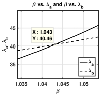
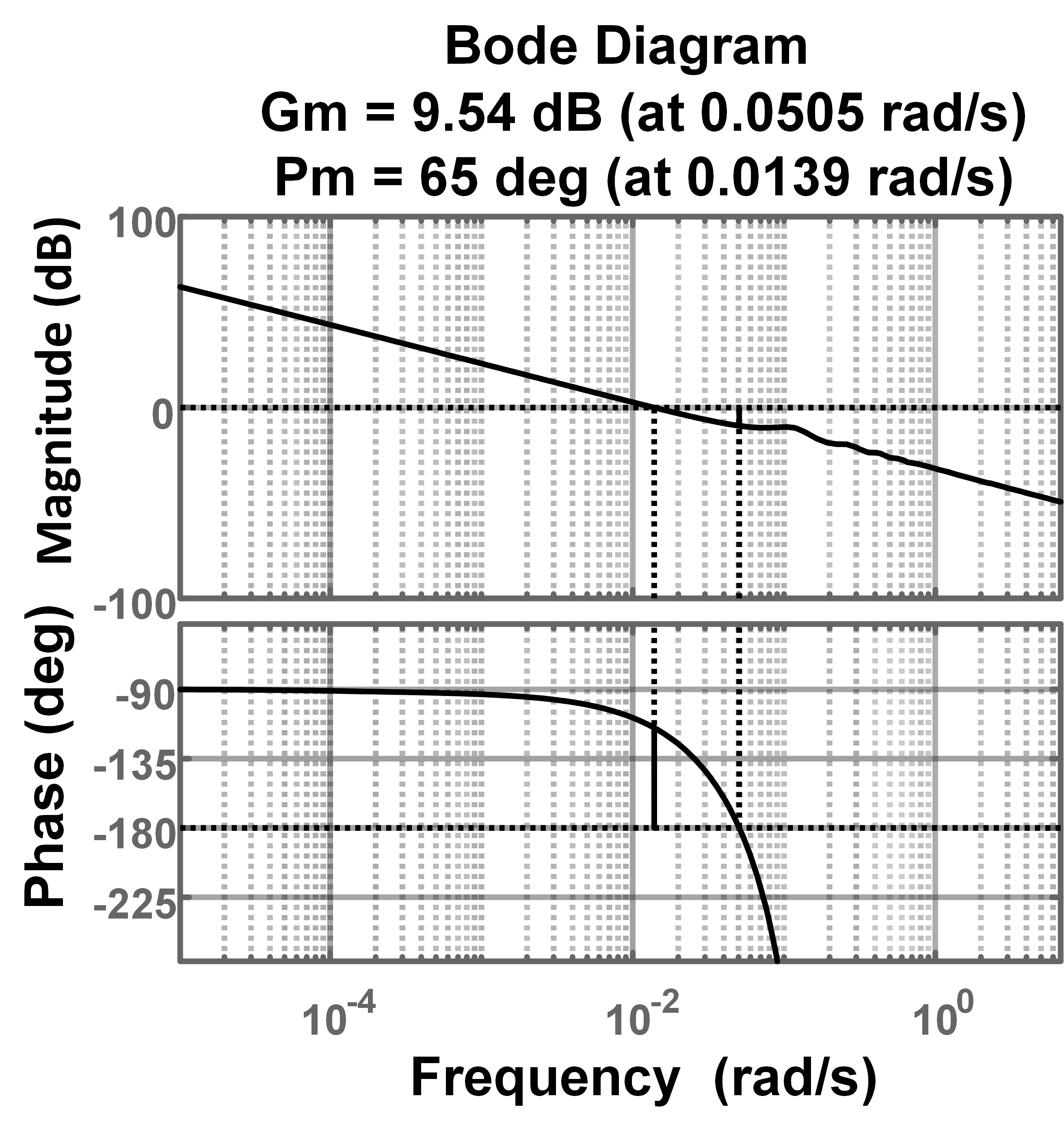
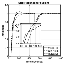
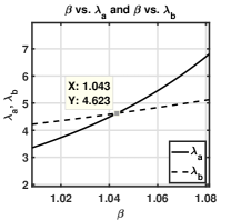
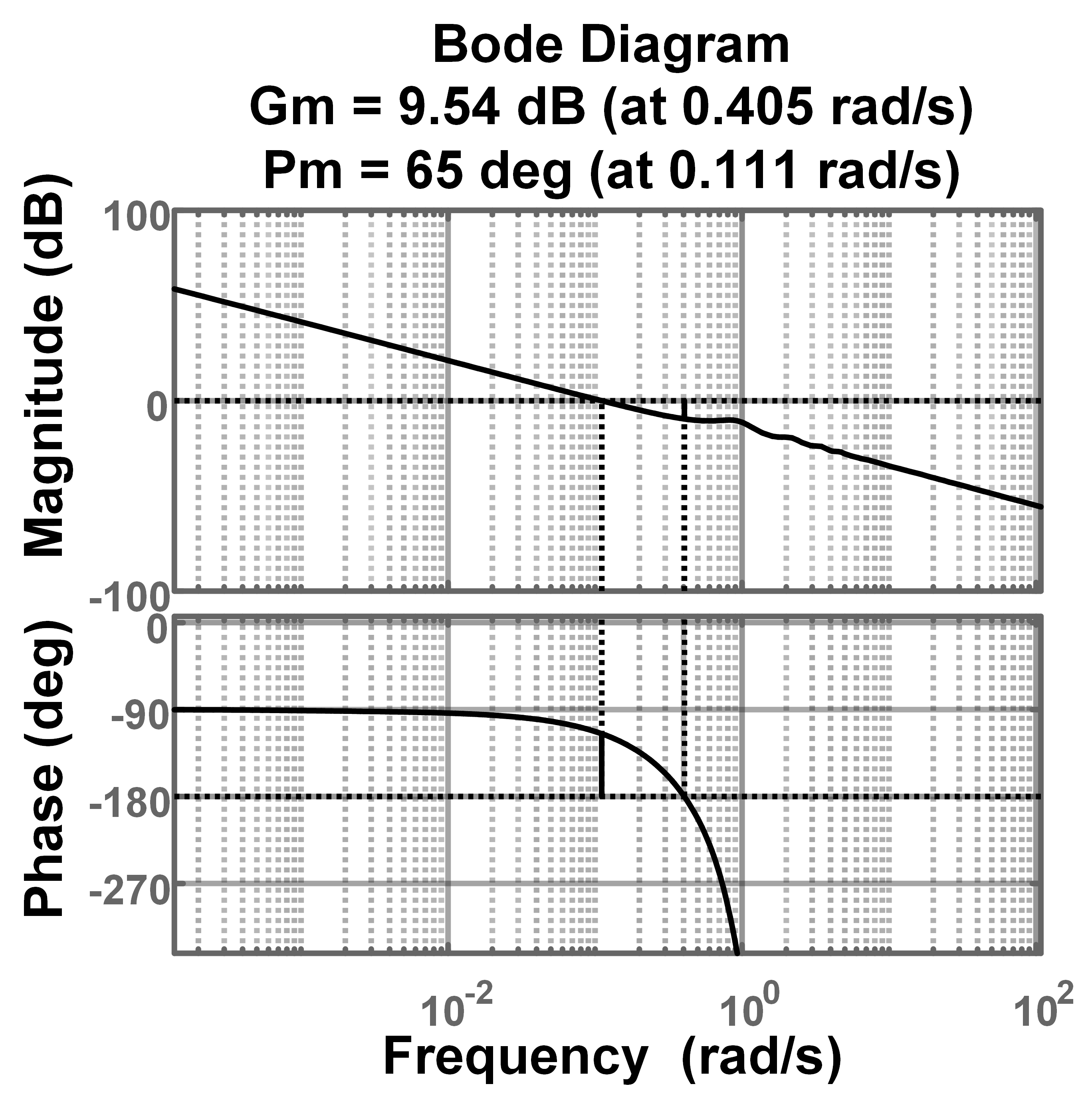
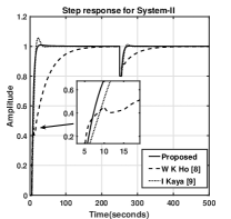
Figure 6: Figure ($a_{1}$) and ($b_{1}$), $\beta\,vs.\,\lambda_{a}$ and $\beta\,vs.\,\lambda_{b}$. ($a_{2}$) and ($b_{2}$), Bode plot with proposed controller and ($a_{3}$) and ($b_{3}$), step response to compare different methods for system-I and II respectively. In $(b_{1})$ and $b_{2}$, Gm is $A_{m}$ and Pm is $\phi_{m}$.

Desired $A_{m}=3$ and desired $\phi_{m}=65\deg(=1.1345rad)$. Using controller design steps in Section-2.8, $\beta_{x1}=0.6389$ and $\beta_{y2}=1.2778$ are evaluated. Therefore, $\beta_{{\omega_{g}}}\in(0.6389,1.2778)$. The controller parameters are obtained as $\beta^{\star}=1.043$ and $\lambda^{\star}=40.46$ (see Fig.6)($a_{1}$). Corresponding to $\beta=1.043$, we get $\omega_{g}^{\star}=0.01391$ and $\omega_{p}^{\star}=0.05066$. The bode plot in Fig.6($b_{1}$) shown that the simulation results are obtained as per theoretical calculations.

For $A_{m}=3$, [5] will provide $\phi_{m}=74.31\deg(=1.2970rad)$ whereas [4] will provide $\phi_{m}=60\deg(=1.0472rad)$. In case of [5], the obtained parameter are $\beta=1$ and $\lambda=57.35$, which results in $PID=5.05+0.03/s+88.9945s$. Whereas, for [4], $\beta=1$ and $\lambda=36.39$, resulting in $PI=4.5056+148/s$. The step response is shown in Fig.6($c_{1}$). It is clear from the plot that the proposed method works best among the three.

3.2 Example-II

A delay dominant process model is considered from [8], which is

$${G_{p}}\left(s\right)=\frac{{1}}{{0.5s+1}}{e^{-5s}}$$ (82)

The controller is designed for $A_{m}=3$ and $\phi_{m}=65\deg(=1.1345rad)$. Following steps in Section-2.8, $\beta_{x1}=0.6389$ and $\beta_{y2}=1.2778$ are evaluated. Therefore, $\beta_{{\omega_{g}}}\in(0.6389,1.2778)$. The controller parameters obtained are $\beta^{\star}=1.043$ and $\lambda^{\star}=4.623$ (see Fig.6($a_{2}$)). Corresponding to $\beta=1.043$, we get $\omega_{g}^{\star}=0.111$ and $\omega_{p}^{\star}=0.405$. The bode plot in Fig.6($b_{2}$) shows that the simulation results are obtained as per the theoretical calculations.

Corresponding to $A_{m}=3$, according to [5] the only possible $\phi_{m}$ is $=74.31\deg(=1.2970rad)$ and according to [4] it is $60\deg(=1.0472rad)$. For [5], $\beta=1$ and $\lambda=7.1691$, giving $PID=0.3103+0.1034/s+0.1293s$ and for [4], $\beta=1$ and $\lambda=4.5433$, giving $PI=0.0524+0.5/s$. The step response is shown in Fig.6($c_{2}$). It is clear from the plot that the proposed method works best among the three.

4 Discussion and Conclusion

An FO-IMC based controller is designed for desired gain margin and phase margin for a FOPTD process model. FO filter is used instead of IO filter in the IMC structure as it provides an additional parameter to tune as compared to a single parameter in IO filter. With only one tuning parameter in IO filter, the range of selection of desired $\phi_{m}$ and $A_{m}$ is limited to a 1-D curve. With two tuning parameters in FO filter, the range of selection of desired $\phi_{m}$ and $A_{m}$ becomes a 2-D surface. Therefore, they can be chosen independently. The controller is designed without any approximation of the delay term appearing in the model of plant. To the best of authors’ knowledge, this is the first attempt made in IMC literature where the controller is designed without any approximation of the delay term in the process model.

The proposed control strategy should be implemented in original IMC structure Fig.1(a). The controller is able to satisfy $\phi_{m}\in(0,\pi)$, $A_{m}>1$ for any $\theta/\tau>0$ which highly enhances the scope of the proposed control strategy.

References

- [1] C. E. Garcia and M. Morari, “Internal model control. a unifying review and some new results,” Industrial & Engineering Chemistry Process Design and Development, vol. 21, no. 2, pp. 308–323, 1982.
- [2] D. Rivera, M. Morari, and S. Skogestad, “Internal model control. 4. pid controller design.” Industrial & Engineering Chemistry, Process Design and Development, vol. 25, no. 1, pp. 252–265, 1 1986.
- [3] M. Morari and E. Zatrioiu, Robust Process Control. Prentice Hall, 1989.
- [4] I. Kaya, “Tuning pi controllers for stable processes with specifications on gain and phase margins,” ISA Transactions, vol. 43, no. 2, pp. 297 – 304, 2004.
- [5] W. K. Ho, T. H. Lee, H. P. Han, and Y. Hong, “Self-tuning imc-pid control with interval gain and phase margins assignment,” IEEE Transactions on Control Systems Technology, vol. 9, no. 3, pp. 535–541, May 2001.
- [6] C.-W. Chu, B. E. Ydstie, and N. V. Sahinidis, “Optimization of imc-pid tuning parameters for adaptive control: Part 1,” in 21st European Symposium on Computer Aided Process Engineering, ser. Computer Aided Chemical Engineering, E. Pistikopoulos, M. Georgiadis, and A. Kokossis, Eds. Elsevier, 2011, vol. 29, pp. 758 – 762.
- [7] W. K. Ho, C. C. Hang, and J. H. Zhou, “Performance and gain and phase margins of well-known pi tuning formulas,” IEEE Transactions on Control Systems Technology, vol. 3, no. 2, pp. 245–248, June 1995.
- [8] Y.-C. Tian and F. Gao, “Compensation of dominant and variable delay in process systems,” Industrial & Engineering Chemistry Research, vol. 37, no. 3, pp. 982–986, 1998.