Extending Transition Path Theory:
Periodically-Driven and Finite-Time Dynamics

Abstract

Given two distinct subsets $A,B$ in the state space of some dynamical system, Transition Path Theory (TPT) was successfully used to describe the statistical behavior of transitions from $A$ to $B$ in the ergodic limit of the stationary system. We derive generalizations of TPT that remove the requirements of stationarity and of the ergodic limit, and provide this powerful tool for the analysis of other dynamical scenarios: periodically forced dynamics and time-dependent finite-time systems. This is partially motivated by studying applications such as climate, ocean, and social dynamics. On simple model examples we show how the new tools are able to deliver quantitative understanding about the statistical behavior of such systems. We also point out explicit cases where the more general dynamical regimes show different behaviors to their stationary counterparts, linking these tools directly to bifurcations in non-deterministic systems.

Keywords Transition Path Theory, Markov chains, time-inhomogeneous process, periodic driving, finite-time dynamics

1 Introduction

The understanding of when and how dynamical transitions, such as tipping processes, happen is important for many systems from physics, biology [noe2009constructing], ecology [scheffer2001catastrophic, hastings2018transient], the climate [lenton2008tipping, lenton2013environmental] and the social sciences [nyborg2016social, otto2020social].

If the system dynamics can be modelled by a stationary Markov process running for infinite time, Transition Path Theory (TPT) provides a rigorous approach for studying the transitions from one subset $A$ to another subset $B$ of the state space. The main tool of Transition Path Theory [weinan2006towards, metzner2009transition] are the forward and backward committor probabilities telling us the probability of the Markov process to next commit to (i.e., hit) $B$ relative to $A$, either forward or backward in time. Given these committor probabilities, one can derive important statistics of the ensemble of reactive trajectories (i.e., of the collection of all possible paths of the Markov process that start in $A$ and end in $B$), such as

• the density of reactive trajectories telling us about the bottlenecks during transitions,

• the current of reactive trajectories indicating the most likely transition channels,

• the rate of reactive trajectories leaving $A$ or entering $B$, and

• the mean duration of reactive trajectories.

Other approaches that characterize the ensemble of transition paths, on the one hand, place the focus elsewhere: For instance, in Transition Path Sampling [BolhuisChandlerDellago2002] one is interested in directly sampling trajectories of the reactive ensemble. On the other hand, these approaches consider different objects, such as the steepest descent path [ulitsky1990new, czerminski1990self, olender1997yet], the most probable path [olender1996calculation, elber2000temperature, pinski2010transition, Faccioli2010dominant, Beccara2012dominant] (also in temporal networks [ser2015most]), or the first passage path ensemble [von2018statistical] (see also Remark LABEL:rem:non-ergodic_processes).

For many physical, especially molecular, systems that are equilibrated and where transitions happen on a smaller time scale than the observation window, the assumption of a stationary, infinite-time Markov process is reasonable and common practice [noe2009constructing]. For illustration we consider the overdamped Langevin dynamics

$$dX_{t}=-\nabla V(X_{t})dt+\sigma dW_{t}$$

in the triple well landscape $V(x,y)$ (as in Figure 1), and we are interested in the transitions between the deep well $A$ and the other deep well $B$. If the noise intensity $\sigma$ is sufficiently small, then the system tends to spend long times near local minima of deep wells (this behavior is called metastability) and transitions predominantly happen across regions of possibly low values of the potential $V$ (e.g., saddle points). If the system from Figure 1 is stationary and has infinite time for transitioning, the transition channel via the metastable well centered at $(0,1.5)$ is preferred since the barriers are lower and it does not matter that transitions take a very long time due to being stuck in the metastable set.

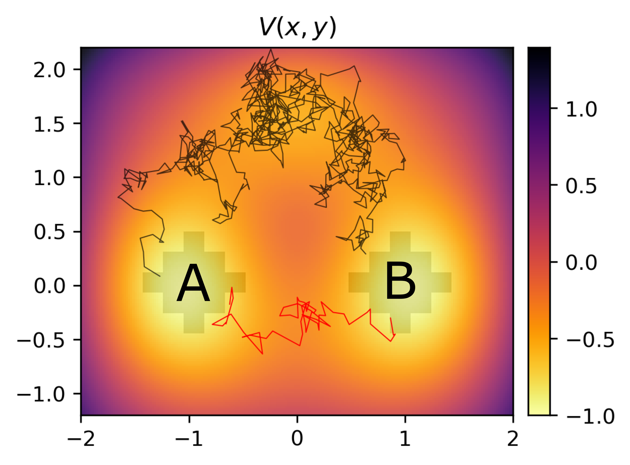
(a)

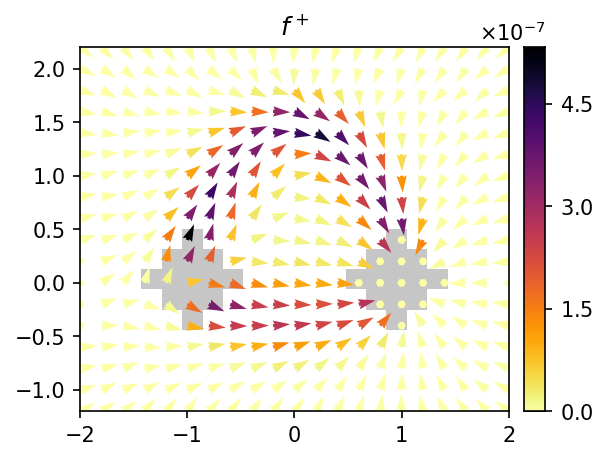
(b)

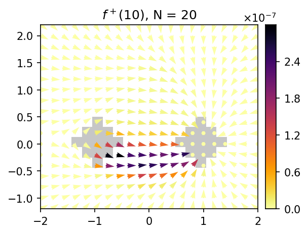
(c)

Figure 1: (a) Triple well potential landscape with two possible reactive trajectories, i.e., transitions from $A$ to $B$, highlighted in black and red. (b) The effective current of reactive trajectories from $A$ to $B$ in infinite time; the channel via the well at $(0,1.5)$ is dominantly taken. (c) The effective current of reactive trajectories restricted to a small time window; the transition channel via the direct barrier between $A$ and $B$ is more likely. More details on the numerical example can be found in Section LABEL:sec:triplewell_ex, but here we chose a smaller noise intensity $\sigma=0.26$.

However, in order to study transitions and tipping paths in different dynamical contexts (e.g., social systems or climate models) which are often characterized by time-dependent (e.g., seasonal) dynamics as well as transitions of interest within a finite time window, the current theory of transition paths has to be extended.

In these applications one might, for instance, ask: What are the possible transition channels from the current state to a desirable and sustainable state of our social or climate system within the next 30 years [steffen2018trajectories, otto2020social]? By requiring the transitions to depart from $A$ and arrive in $B$ within a finite time interval, the affinity of the system taking the different transition channels is altered. This is visualized in the triple well dynamics, Figure 1(c), where now only the lower transition channel passing the high barrier is possible. Whenever the trajectory takes the channel through the upper metastable set (cf. black trajectory in Subfigure (a)), it is stuck there for a long time, and will not reach $B$ anymore within the finite time horizon.

Moreover, systems containing human agents are usually time-inhomogeneous and not equilibrated while climate systems are often affected by seasonal forcing, raising questions such as: What are the likely spreading paths of a contagion in a time-evolving network [pan2011path, brockmann2013hidden, valdano2018epidemic]? What are bottlenecks in the transient dynamics towards the equilibrium state [schonmann1992pattern, hollander2000metastability]? How does tipping occur under the joint effect of noise and parameter changes [ashwin2012tipping, giorgini2019predicting] or periodic forcing [herrmann2005exit]?

In this paper we generalize TPT to a broader class of dynamical scenarios. In particular, we focus on two generalizations which we consider as natural but not exclusive building blocks for these more general cases: (a) periodically forced infinite-time system and (b) arbitrary time-inhomogeneous finite-time system.

We start in Section 2 by formulating the general setting of TPT for Markov chains $(X_{n})_{n\in\mathbb{T}}$ on a finite state space by introducing time-dependent forward committor functions $q^{+}_{i}(n)$, giving the probability within the time horizon $\mathbb{T}$ to next commit to $B$ and not $A$ conditional on being in $X_{n}=i$, as well as time-dependent backward committor functions $q^{-}_{i}(n)$, both of which are needed for computing the desired statistics of the transitions from $A$ to $B$.

We then in more detail work out the following main cases.

• Under the assumption of stationary, infinite-time dynamics, it is known [weinan2006towards, metzner2009transition] that the committor functions are time-independent $q^{+}(n)=q^{+}$ by stationarity and solve the following linear system

  $$\left\{\begin{array}[]{rcll}q_{i}^{+}&=&\sum\limits_{j\in\mathbb{S}}\,P_{ij}\,q_{j}^{+}&i\in(A\cup B)^{c}\\ q_{i}^{+}&=&0&i\in A\\ q_{i}^{+}&=&1&i\in B\\ \end{array}\right.$$ (1)

  where $P=(P_{ij})_{i,j\in\mathbb{S}}$ is the transition matrix. Similarly all the transition statistics are time-independent and by ergodicity the statistics can also be found by averaging along one infinitely long equilibrium trajectory [weinan2006towards, metzner2009transition]. In Section 3 we recall the theory [weinan2006towards, metzner2009transition] from a different point of view. Instead of defining all quantities in terms of trajectory-wise time-averages, we prove by using the Markov property that they can be written in terms of the committors and the stationary distribution. Further, we extend the theory by Lemma 3.5 decomposing the committors into path probabilities.

• In Section LABEL:sec:tpt_periodic we derive the committors and transition statistics for periodically varying dynamics with a period of length $M$ that are equilibrated (i.e., the law of the chain is also periodic). It follows that the committors are periodically varying $q^{+}(n)=q^{+}_{m}$ whenever $n=m$ modulo $M$, and we show that the committors solve the following linear system with periodic boundary conditions in time $q^{+}_{0}=q^{+}_{M}$

  $$\left\{\begin{array}[]{rcll}q_{m,i}^{+}&=&\sum\limits_{j\in\mathbb{S}}\,P_{m,ij}\,q_{m+1,j}^{+}&i\in(A\cup B)^{c}\\ q_{m,i}^{+}&=&0&i\in A\\ q_{m,i}^{+}&=&1&i\in B\\ \end{array}\right.$$ (2)

  where $P_{m}=(P_{m,ij})_{i,j\in\mathbb{S}}$ is the transition matrix at time $n=m$ modulo $M$. This is consistent with the previous case when choosing a period of length $M=1$.

• In Section LABEL:sec:tpt_finite we derive the committor equations and transition statistics for general time-inhomogeneous Markov chains $(X_{n})_{n\in\mathbb{T}}$ on a finite-time interval $\mathbb{T}=\{0,\dots,N-1\}$ defined by the transition probabilities $P(n)=(P_{ij}(n))_{i,j\in\mathbb{S}}$ and an initial density $\lambda(0)$. The forward committor $q^{+}(n)$ for a finite-time Markov chain satisfies the following iterative system of equations:

  $$\left\{\begin{array}[]{rcll}q_{i}^{+}(n)&=&\sum\limits_{j\in\mathbb{S}}\,P_{ij}(n)\,q_{j}^{+}(n+1)&i\in(A\cup B)^{c}\\ q_{i}^{+}(n)&=&0&i\in A\\ q_{i}^{+}(n)&=&1&i\in B\end{array}\right.$$ (3)

  with final condition $q^{+}_{i}(N-1)=\mathbbm{1}_{B}(i)$. The transition statistics depend on the current time point in the time interval and can be related to an average over the ensemble of reactive trajectories. We also show consistency, i.e., that given a stationary process on a finite time interval, the committors and statistics converge to their classical counterparts (i) in the infinite time limit.

We note that in the stationary regime, committor functions have been used for finding basins of attraction of stochastic dynamics [Kol11, KoVo14, lindner2019stochastic], as reaction coordinates [lu2014exact], as basis functions in the core-set approach  [schutte2011markov, sarich2011projected, schutte2013metastability] and for studying modules and flows in networks [djurdjevac2011random, cameron2014flows]. We expect our results to enable similar uses for the time-dependent regime.

The theoretical results from this paper are accompanied by numerical studies on two toy examples, a network of $5$ nodes with time-varying transition probabilities, and a discrete model of the overdamped Langevin dynamics in a triple well potential with time-dependent forcing (as in Figure 1). In these examples we will particularly show to what extent time-dependent dynamics or finite-time restrictions affect the transition statistics in contrast to those in stationary, infinite time dynamics. The TPT-related objects derived here allow for a quantitative assessment of the dominant statistical behavior in complicated dynamical regimes:

• By adding a periodic forcing to the stationary dynamics, the reaction channels are perturbed and new transition paths, that were not possible before, can appear (see Example 2 and 7).

• By restricting the stationary dynamics with matrix $P$ to a finite-time window (cf. Example 3 and 8), only transitions within this window are allowed and the average rate of transitions is much lower than in the infinite-time situation. By additionally applying a forcing (cf. Example 4), the system is not equilibrated anymore and we can get a higher average rate of transitions than without forcing, although we set the time-dependent transition matrix $P(n)$ such that its time-average equals the transition matrix $P$ of the stationary case. A similar approach is used in rare events simulation where the system is pushed by an optimal non-equilibrium forcing under which the rare events become more likely [Hartmann2012optimal, Hartmann2014characterization].

• The finite-time case can also be employed for studying qualitative changes in the transition dynamics when parameters are perturbed. In Example 9, we exemplarily show that by increasing the finite-time interval length $N$, the transition dynamics change qualitatively, even though the dynamics are stationary. Thus, TPT can be used as a quantitative tool describing bifurcations in non-stationary non-deterministic systems.

The code used for the examples is available on Github at www.github.com/LuzieH/pytpt.

2 Preliminaries and General Setup

The objective of Transition Path Theory (TPT) is to understand the mechanisms by which noise-induced transitions of a Markov chain $(X_{n})_{n\in\mathbb{T}}$ from one subset of the state space $A\subset\mathbb{S}$ to another subset $B\subset\mathbb{S}$ take place. $A$ and $B$ are chosen as two non-empty, disjoint subsets of the finite state space $\mathbb{S}$, such that the transition region $C:=(A\cup B)^{c}$ is also non-empty. Since historically in TPT one thinks of $A$ as the reactant states of a system, $B$ as the product states and the transitions from $A$ to $B$ as reaction events, we call the pieces of a trajectory that connect $A$ to $B$ by the name reactive trajectories. Each reactive trajectory contains the successive states in $C$ visited during a transition that starts in $A$ and ends in $B$, see Figure 2, and we are interested in gathering dynamical information about the ensemble of reactive trajectories.

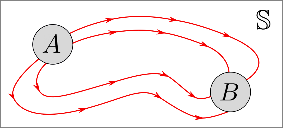
Figure 2: Reactive trajectories, i.e., excursions of trajectories that start in $A$ and end in $B$.

In this paper, we are interested not only in Markov chains living on the infinite time frame $\mathbb{T}=\mathbb{Z}$ but also those on finite time intervals $\mathbb{T}=\{0,1,\dots,N-1\}$, that is where the transitions from $A$ to $B$ have to take place during a finite time frame $\mathbb{T}$. Moreover, we also consider non-stationary dynamics. This either means

• that the system is in the transient phase towards equilibrium but otherwise has a time-independent transition matrix, or

• that the dynamical rules (the transition matrices) are varying in time, as well as

• that we are dealing with time-varying sets $A$ and $B$ (see the comment in Section LABEL:sec:com_periodic for the case of periodic dynamics and Remark LABEL:rem:space_time_set_finite for finite-time dynamics).

In this section, we will define the committor functions and show how they can be used to derive important statistics of the ensemble of reactive trajectories, this entails, e.g., the frequency of transitions, the most important transition channels and where the process on the way to $B$ gets stuck or spends most of its time. Thereby we will keep everything general enough for time-dependent and finite-time dynamics and for the moment only need to assume the Markovianity of the chain $(X_{n})_{n\in\mathbb{T}}$ and that the distribution $\mathbb{P}(X_{n}=i)$ and time-dependent transition rule $P(n)=(\mathbb{P}(X_{n+1}=j|X_{n}=i))_{i,j\in\mathbb{S}}$ is given for all $n\in\mathbb{T}$.

Later, the results from this section will be applied to the special cases of (i) infinite-time, stationary dynamics (Section 3), (ii) infinite-time, periodic dynamics (Section LABEL:sec:tpt_periodic) and (iii) finite-time, time-dependent systems (Section LABEL:sec:tpt_finite), where we will also prove the existence of committors and give the linear system of equations they are solving. These three are just some selected special cases, other interesting cases of systems are, e.g., stochastic regime-switching (see the Remark LABEL:rem:switching).

2.1 Committor Equations

All of the transition statistics and characteristics can be computed from the committor probabilities, therefore we will start by defining them. The forward committor is the probability that the Markov chain, currently in some state $i$, will next go to set $B$ and not to $A$. The backward committor is the same for the time-reversed Markov chain, i.e., the probability that the time-reversed process will next hit $A$ and not $B$, or equivalently, the probability that the chain last came from $A$ and not $B$.

More precisely, the forward committor $q^{+}(n)=(q^{+}_{i}(n))_{i\in\mathbb{S}}$ gives the probability that the process starting in $i\in\mathbb{S}$ at time $n\in\mathbb{T}$ reaches at next within $\mathbb{T}$ first $B$ and not $A$. We write

$$\begin{split}q_{i}^{+}(n):=\mathbb{P}(\tau_{B}^{+}(n)<\tau_{A}^{+}(n)\,|\,X_{n}=i),\end{split}$$ (4)

where the first entrance time of a set $S\subset\mathbb{S}$ after or at time $n\in\mathbb{T}$ is given by

$$\tau_{S}^{+}(n):=\inf\{k\in\mathbb{T}\text{ s.t. }k\geq n,X_{k}\in S\},\ \inf\varnothing:=\infty.$$

The backward committor $q^{-}(n)=(q^{-}_{i}(n))_{i\in\mathbb{S}}$ gives the probability that the trajectory arriving at time $n\in\mathbb{T}$ in state $i\in\mathbb{S}$ last within $\mathbb{T}$ came from $A$ not $B$,

$$\begin{split}q_{i}^{-}(n):=\mathbb{P}(\tau_{A}^{-}(n)>\tau_{B}^{-}(n)\,|\,X_{n}=i),\end{split}$$ (5)

where the last exit time of a set $S$ before time or at time $n$ is given by

$$\tau_{S}^{-}(n):=\sup\{k\in\mathbb{T}\text{ s.t. }k\leq n,X_{k}\in S\},\ \sup\varnothing:=-\infty.$$

Note that the first entrance and last exit times are stopping times with respect to the forward and time-reversed process [RiberaBorrell2019, Lemma 3.1.1]. The time-reversed process will be introduced in the following sections for infinite-time and finite-time Markov chains.

The forward committor, as it is defined, only considers trajectory pieces arriving at $B$ within the time horizon $\mathbb{T}$, similarly, the backward committor only considers excursions that left $A$ within $\mathbb{T}$.

2.2 Transition Statistics

We will now define statistical objects that characterize the ensemble of reactive trajectories from subset $A$ to $B$ and see that they can be computed using the committor probabilities and the Markovianity assumption.

The first two objects, the distribution of reactive trajectories $\mu^{AB}(n)$ and its normalized version $\hat{\mu}^{AB}(n)$, tell us where the reactive trajectories are most likely to be found, i.e., where the transitioning trajectories spend most of their time.

Definition 2.1.

The distribution of reactive trajectories $\mu^{AB}(n)=(\mu^{AB}_{i}(n))_{i\in\mathbb{S}}$ for $n\in\mathbb{T}$ gives the joint probability that the Markov chain is in a state $i$ at time $n$ while transitioning from $A$ to $B$:

$$\mu^{AB}_{i}(n):=\mathbb{P}(X_{n}=i,\tau_{A}^{-}(n)>\tau_{B}^{-}(n),\tau_{B}^{+}(n)<\tau_{A}^{+}(n)).$$

Note that $\mu^{AB}_{i}(n)=0$ for $i\notin C$, i.e., we only get information about the density of transitions passing through $C$. Direct transitions from $A$ to $B$ are neglected, and in general assumed not to exist.

Theorem 2.2.

For a general Markov chain $(X_{n})_{n\in\mathbb{T}}$ with committors $q^{+}(n)$, $q^{-}(n)$, the distribution of reactive trajectories can be expressed as

$$\begin{split}\mu^{AB}_{i}(n)&=q_{i}^{-}(n)\,\mathbb{P}(X_{n}=i)\,q_{i}^{+}(n).\end{split}$$

Proof.

We can compute

$$\begin{split}\mu^{AB}_{i}(n)&=\mathbb{P}(\tau_{A}^{-}(n)>\tau_{B}^{-}(n),\tau_{B}^{+}(n)<\tau_{A}^{+}(n)\,|\,X_{n}=i)\,\mathbb{P}(X_{n}=i)=q_{i}^{-}(n)\,q_{i}^{+}(n)\,\mathbb{P}(X_{n}=i)\end{split}$$

by conditioning on $\{X_{n}=i\}$, and by using independence of the two events $\{\tau_{A}^{-}(n)>\tau_{B}^{-}(n)\}$, $\{\tau_{B}^{+}(n)<\tau_{A}^{+}(n)\}$ given $\{X_{n}=i\}$, which follows from the Markov property. ∎

The distribution $\mu^{AB}(n)$ is not normalized but can easily be normalized by dividing $\mu^{AB}(n)$ by the probability to be on a transition at time $n$,

$$Z^{AB}(n):=\sum_{j\in C}\mu^{AB}_{j}(n)=\mathbb{P}(\tau_{A}^{-}(n)>\tau_{B}^{-}(n),\tau_{B}^{+}(n)<\tau_{A}^{+}(n)),$$

to give a probability distribution on $\mathbb{S}$:

Definition 2.3.

Whenever $\mathbb{P}(\tau_{A}^{-}(n)>\tau_{B}^{-}(n),\tau_{B}^{+}(n)<\tau_{A}^{+}(n))>0$ for $n\in\mathbb{T}$, we can define the normalized distribution of reactive trajectories at time $n\in\mathbb{T}$ by

$$\hat{\mu}^{AB}_{i}(n):=\mathbb{P}(X_{n}=i|\tau_{A}^{-}(n)>\tau_{B}^{-}(n),\tau_{B}^{+}(n)<\tau_{A}^{+}(n))$$

giving the density of states in which trajectories transitioning from $A$ to $B$ spend their time.

The next object tells us about the average number of jumps from $i$ to $j$ during one time step (i.e., the probability flux) while the trajectory is on its way from $A$ to $B$:

Definition 2.4.

The current of reactive trajectories $f^{AB}(n)=(f^{AB}_{ij}(n))_{i,j\in\mathbb{S}}$ at time $n\in\mathbb{T}$ gives the average flux of trajectories going through $i$ at time $n\in\mathbb{T}$ and $j$ at time $n+1\in\mathbb{T}$ consecutively while on their way from $A$ to $B$:

$$f^{AB}_{ij}(n):=\mathbb{P}(X_{n}=i,X_{n+1}=j,\tau_{A}^{-}(n)>\tau_{B}^{-}(n),\tau_{B}^{+}(n+1)<\tau_{A}^{+}(n+1))$$

Theorem 2.5.

The current of reactive trajectories for a Markov chain $(X_{n})_{n\in\mathbb{T}}$ with transition probabilities $P(n)$ and committors $q^{+}(n)$, $q^{-}(n)$, is given by

$$\begin{split}f^{AB}_{ij}(n)=q_{i}^{-}(n)\,\mathbb{P}(X_{n}=i)\,P_{ij}(n)\,q^{+}_{j}(n+1)\end{split}$$

Proof.

The reactive current can be computed as

$$\begin{split}f^{AB}_{ij}(n)&=\mathbb{P}(X_{n+1}=j,\tau_{A}^{-}(n)>\tau_{B}^{-}(n),\tau_{B}^{+}(n+1)<\tau_{A}^{+}(n+1)|X_{n}=i)\,\mathbb{P}(X_{n}=i)\\ &=\mathbb{P}(X_{n+1}=j,\tau_{B}^{+}(n+1)<\tau_{A}^{+}(n+1)|X_{n}=i)\,\mathbb{P}(\tau_{A}^{-}(n)>\tau_{B}^{-}(n)|X_{n}=i)\,\mathbb{P}(X_{n}=i)\\ &=\mathbb{P}(X_{n+1}=j|X_{n}=i)\,\mathbb{P}(\tau_{B}^{+}(n+1)<\tau_{A}^{+}(n+1)|X_{n+1}=j,X_{n}=i)\,q_{i}^{-}(n)\,\mathbb{P}(X_{n}=i)\\ &=q_{i}^{-}(n)\,\mathbb{P}(X_{n}=i)\,P_{ij}(n)\,q^{+}_{j}(n+1),\end{split}$$

by first conditioning on $\{X_{n}=i\}$, then by independence of $\{X_{n+1}=j,\tau_{B}^{+}(n+1)<\tau_{A}^{+}(n+1)\}$ and $\{\tau_{A}^{-}(n)>\tau_{B}^{-}(n)\}$ given $\{X_{n}=i\}$, by conditioning on $\{X_{n+1}=j\}$, and last by the Markov property. ∎

Let us note that the reactive current also counts the transitions going directly from $i\in A$ to $j\in B$, these are not accounted for in the reactive distribution which only accounts for transitions passing the region $(A\cup B)^{c}$.

In order to eliminate information about detours of reactive trajectories, we define:

Definition 2.6.

The effective current of reactive trajectories $f^{+}(n)=(f^{+}_{ij}(n))_{i,j\in\mathbb{S}}$ at time $n\in\mathbb{T}$ gives the net amount of reactive current going through $i$ at time $n\in\mathbb{T}$ and $j$ at time $n+1\in\mathbb{T}$ consecutively,

$$f^{+}_{ij}(n):=\max\{f^{AB}_{ij}(n)-f^{AB}_{ji}(n),0\}.$$

Ultimately, the effective current of reactive trajectories can be used to find the dominant transition channels in state space between $A$ and $B$ (see, e.g., [metzner2009transition]).

The current of reactive trajectories only goes out of $A$, not into $A$, moreover the current of reactive trajectories only points into $B$, not out of $B$. Therefore, $A$ can be thought of as a source of reactive trajectories, whereas $B$ acts like their sink. This leads us to our next characteristic of reactive trajectories: by summing the current of reactive trajectories over $A$ we get the the discrete rate of reactive trajectories flowing out of $A$, and by summing the current over $B$, we obtain the rate of inflow into $B$:

Definition 2.7.

For $n,n+1\in\mathbb{T}$, the discrete rate of transitions leaving $A$ at time $n$ is given by

$$k^{A\rightarrow}(n):=\mathbb{P}(X_{n}\in A,\tau_{B}^{+}(n+1)<\tau_{A}^{+}(n+1)),$$

i.e., the probability of a reactive trajectory leaving $A$ at time $n$. When $n-1,n\in\mathbb{T}$, the discrete rate of transitions entering $B$ at time $n$ is given by

$$k^{\rightarrow B}(n):=\mathbb{P}(X_{n}\in B,\tau_{A}^{-}(n-1)>\tau_{B}^{-}(n-1)),$$

i.e., the probability of a reactive trajectory entering $B$ at time $n$.

Theorem 2.8.

For a Markov chain $(X_{n})_{n\in\mathbb{T}}$ with current of reactive trajectories $f^{AB}(n)$, we find the discrete rates to be

$$\begin{split}k^{A\rightarrow}(n)&=\sum_{i\in A,j\in\mathbb{S}}f^{AB}_{ij}(n)\\ k^{\rightarrow B}(n)&=\sum_{i\in\mathbb{S},j\in B}f^{AB}_{ij}(n-1).\\ \end{split}$$ (6)

Proof.

We can compute by using the law of total probability

$$\begin{split}\sum_{i\in A,j\in\mathbb{S}}f^{AB}_{ij}(n)&=\sum_{i\in A,j\in\mathbb{S}}\mathbb{P}(X_{n}=i,X_{n+1}=j,\tau_{A}^{-}(n)>\tau_{B}^{-}(n),\tau_{B}^{+}(n+1)<\tau_{A}^{+}(n+1))=k^{A\rightarrow}(n)\\ \sum_{i\in\mathbb{S},j\in B}f^{AB}_{ij}(n-1)&=\sum_{i\in\mathbb{S},j\in B}\mathbb{P}(X_{n-1}=i,X_{n}=j,\tau_{A}^{-}(n-1)>\tau_{B}^{-}(n-1),\tau_{B}^{+}(n)<\tau_{A}^{+}(n))=k^{\rightarrow B}(n).\end{split}$$ (7)

∎

3 TPT for Stationary, Infinite-time Markov Chains

TPT was originally designed for stationary, infinite-time Markov processes [weinan2006towards, metzner2009transition], that are often used as models for molecular systems [noe2009constructing]. Here we will recall that theory by using the results from the previous section and equip it with some new results (e.g. Lemma 3.5) that will be needed later.

3.1 Setting

We begin with describing the processes of interest in this section.

Assumption 3.1.

We consider a Markov chain $(X_{n})_{n\in\mathbb{Z}}$ taking values in a discrete and finite state space $\mathbb{S}$, the time-discrete jumps between states $i\in\mathbb{S}$ and $j\in\mathbb{S}$ occur with probability

$$P_{ij}:=\mathbb{P}(X_{n+1}=j|X_{n}=i)$$

stored in the row-stochastic transition matrix $P=(P_{ij})_{i,j\in\mathbb{S}}$. We assume that the process is irreducible, and ergodic with respect to the unique, strictly positive invariant distribution $\pi=(\pi_{i})_{i\in\mathbb{S}}$ (also called stationary distribution interchangeably) solving $\pi^{\top}=\pi^{\top}P$.

The time-reversed process $(X^{-}_{n})_{n\in\mathbb{Z}}$, $X^{-}_{n}:=X_{-n}$ traverses the chain backwards in time. It is also a Markov chain [RiberaBorrell2019, Thm 2.1.19] and stationary with respect to the same invariant distribution. The transition probabilities of the time-reversed process $P^{-}=(P^{-}_{ij})_{i,j\in\mathbb{S}}$ with entries

$$P^{-}_{ij}:=\mathbb{P}(X^{-}_{-n+1}=j|X^{-}_{-n}=i)=\mathbb{P}(X_{n-1}=j|X_{n}=i)$$

can be found from expressing the flux in two ways,

$$\mathbb{P}(X_{n}=i,X_{n+1}=j)=P_{ij}\pi_{i}=P^{-}_{ji}\pi_{j}.$$

3.2 Committor Probabilities

Due to stationarity of the chain (Assumption 3.1), the law of the chain is the same for all times, and we simply have that the committors (4) and (5) are time-independent $q_{i}^{+}(n)=q_{i}^{+}$, similarly $q_{i}^{-}(n)=q_{i}^{-}$ for all $n$.

The forward and backward committors can be found by solving a linear matrix equation of size $|C|$ with appropriate boundary conditions [norris1998markov, Chapter 1.3].

Theorem 3.2.

The forward committor for a Markov chain according to Assumption 3.1 with transition probabilities $P=(P_{ij})_{i,j\in\mathbb{S}}$ satisfies the following linear system

$$\left\{\begin{array}[]{rcll}q_{i}^{+}&=&\sum\limits_{j\in\mathbb{S}}\,P_{ij}\,q_{j}^{+}&i\in C\\ q_{i}^{+}&=&0&i\in A\\ q_{i}^{+}&=&1&i\in B.\\ \end{array}\right.$$ (8)

Analogously for the backward committor, we have to solve the following linear system

$$\left\{\begin{array}[]{rcll}q_{i}^{-}&=&\sum\limits_{j\in\mathbb{S}}\,P^{-}_{ij}\,q_{j}^{-}&i\in C\\ q_{i}^{-}&=&0&i\in B\\ q_{i}^{-}&=&1&i\in A.\\ \end{array}\right.$$ (9)

Proof.

From the definition of the committors (4), it immediately follows that we have $q_{i}^{+}=0$ for $i\in A$ since we always have $\tau_{A}^{+}(n)=n$, while $\tau_{B}^{+}(n)>n$. Analogously we have $q_{i}^{+}=1$ for $i\in B$ since in that case $\tau_{A}^{+}(n)>n$ and $\tau_{B}^{+}(n)=n$. For the committor at node $i$ in the transition region $C$, we can sum the forward committor at all the other states $j$ weighted with the transition probability to transition from $i$ to $j$. This follows from

$$\begin{split}q_{i}^{+}&=\mathbb{P}(\tau_{B}^{+}(n)<\tau_{A}^{+}(n)|X_{n}=i)=\sum_{j\in\mathbb{S}}\mathbb{P}(X_{n+1}=j,\tau_{B}^{+}(n)<\tau_{A}^{+}(n)|X_{n}=i)\\ &=\sum_{j\in\mathbb{S}}\mathbb{P}(X_{n+1}=j|X_{n}=i)\mathbb{P}(\tau_{B}^{+}(n)<\tau_{A}^{+}(n)|X_{n+1}=j,X_{n}=i)\\ &=\sum_{j\in\mathbb{S}}\mathbb{P}(X_{n+1}=j|X_{n}=i)\mathbb{P}(\tau_{B}^{+}(n+1)<\tau_{A}^{+}(n+1)|X_{n+1}=j,X_{n}=i)=\sum_{j\in\mathbb{S}}P_{ij}q_{j}^{+}\end{split}$$

first using the law of total probability, then conditioning on $\{X_{n+1}=j\}$, using that at time $n$ the chain is in $i\in C$ and thus $\tau_{A}^{+}(n),\tau_{B}^{+}(n)\geq n+1$, and last using the Markov property.

For the backward committor equations we can proceed in a similar way, by additionally using the time-reversed process. ∎

Remark 3.3.

If the Markov chain in addition is reversible, i.e., if $P_{ij}\pi_{i}=P_{ji}\pi_{j}$ (equivalently, $P^{-}_{ij}=P_{ij}$) holds, then it follows from Theorem 3.2 that the forward and backward committor are related by $q_{i}^{+}=1-q_{i}^{-}$.

The following lemma provides us with the necessary condition such that existence and uniqueness of the committors is guaranteed. For a proof see [RiberaBorrell2019, Lemma 3.2.4] or [norris1998markov, Chapter 4.2].

Lemma 3.4.

If $P$ is irreducible, then the two problems (8) and (9) each have a unique solution.

There is a second characterization of the committors in the transition region using path probabilities, as summarized in the following lemma. The proof can be found in the Appendix LABEL:app:proofs.

Lemma 3.5.

For any $i\in C$, the forward committor can also be specified as the probability of all possible paths starting from node $i$ that reach the set $B$ before $A$

$$\begin{split}q_{i}^{+}&=\sum_{\tau\in\mathbb{Z}^{+}}\sum_{\begin{subarray}{c}i_{1}\dots i_{\tau-1}\in C\\ i_{\tau}\in B\end{subarray}}P_{ii_{1}}\cdots P_{i_{\tau-1}i_{\tau}}.\end{split}$$ (10)

Similarly for any $i\in C$, the backward committor can also be understood as the sum of path probabilities of all possible paths arriving at node $i$ that last came from $A$ and not $B$

$$\begin{split}q_{i}^{-}&=\sum_{\tau\in\mathbb{Z}^{-}}\sum_{\begin{subarray}{c}i_{\tau}\in A\\ i_{\tau+1}\dots i_{-1}\in C\end{subarray}}P^{-}_{i_{\tau+1}i_{\tau}}\cdots P^{-}_{ii_{-1}}.\end{split}$$ (11)

3.3 Transition Statistics

The committor, the distribution, and the transition probabilities are time-independent, thus the statistics from Section 2.2 are time-independent. We write the distribution of reactive trajectories (Theorem 2.2) as $\mu^{AB}=(\mu^{AB}_{i})_{i\in\mathbb{S}}$, where

$$\mu^{AB}_{i}=q_{i}^{-}q_{i}^{+}\ \pi_{i},$$

the normalized distribution as $\hat{\mu}^{AB}=(\hat{\mu}^{AB}_{i})_{i\in\mathbb{S}}$. The current of reactive trajectories (Theorem 2.5) $f^{AB}=(f^{AB}_{ij})_{i,j\in\mathbb{S}}$ is given by

$$f^{AB}_{ij}=q_{i}^{-}\pi_{i}P_{ij}q^{+}_{j},$$

and the effective reactive current is denoted $f^{+}=(f^{+}_{ij})_{i,j\in\mathbb{S}}$.

Theorem 3.6.

For a stationary Markov chain $(X_{n})_{n\in\mathbb{Z}}$ the reactive current out of a node $i\in C$ equals the current flowing into the node $i\in C$, i.e.,

$$\sum_{j\in\mathbb{S}}f^{AB}_{ij}=\sum_{j\in\mathbb{S}}f^{AB}_{ji}.$$ (12)

Further, the the reactive current flowing out of A into $\mathbb{S}$ (equivalently into $C\cup B$) equals the flow of reactive trajectories from $\mathbb{S}$ (equivalently from $C\cup A$) into $B$

$$\sum_{i\in A,j\in\mathbb{S}}f^{AB}_{ij}=\sum_{i\in\mathbb{S},j\in B}f^{AB}_{ij}.$$ (13)

For the proof see the Appendix LABEL:app:proofs.