Universal-RCNN: Universal Object Detector via Transferable Graph R-CNN

Abstract

The dominant object detection approaches treat each dataset separately and fit towards a specific domain, which cannot adapt to other domains without extensive retraining. In this paper, we address the problem of designing a universal object detection model that exploits diverse category granularity from multiple domains and predict all kinds of categories in one system. Existing works treat this problem by integrating multiple detection branches upon one shared backbone network. However, this paradigm overlooks the crucial semantic correlations between multiple domains, such as categories hierarchy, visual similarity, and linguistic relationship. To address these drawbacks, we present a novel universal object detector called Universal-RCNN that incorporates graph transfer learning for propagating relevant semantic information across multiple datasets to reach semantic coherency. Specifically, we first generate a global semantic pool by integrating all high-level semantic representation of all the categories. Then an Intra-Domain Reasoning Module learns and propagates the sparse graph representation within one dataset guided by a spatial-aware GCN. Finally, an Inter-Domain Transfer Module is proposed to exploit diverse transfer dependencies across all domains and enhance the regional feature representation by attending and transferring semantic contexts globally. Extensive experiments demonstrate that the proposed method significantly outperforms multiple-branch models and achieves the state-of-the-art results on multiple object detection benchmarks (mAP: 49.1% on COCO).

Introduction

Figure 1: To identify objects in the upper image from COCO, we could use graph transfer and reasoning across COCO and Visual Genome (VG) (bottom): 1) Objects like “TV”, and “keyboard” in the upper image could help to identify “mouse” and “person”, which requires reasoning and this inspires our Intra-Domain Reasoning Module (blue). 2) Although “table”, “hand”, and “cord” are not annotated in the COCO image but present in VG, recognition of them could help to recognize “mouse”, “keyboard”, which motivates us the Inter-Domain Transfer Module (green to blue).

Object detection is a fundamental vision task that recognizes object’s location and category in an image. Modern object detectors widely benefits autonomous vehicles, surveillance camera, mobile phone, to name a few. According to the individual application, datasets annotated with different categories were created to train a highly-specific and distinct detector e.g. PASCAL VOC (? ?) (20 categories), MSCOCO (? ?) (80 categories) , Visual Genome (VG) (? ?) (more than 33K categories) and BDD (? ?) (10 categories). Those highly-tuned networks have sacrificed the generalization capability and only fit towards each dataset domain. It is impossible to directly adapt the model trained on one dataset to another related task, and thus requires new data annotations and additional computation to train each specific model. In contrast, human is capable of identifying all kinds of objects precisely under complex circumstances and reaches a holistic recognition across different domains. This may be due to the remarkable reasoning and transferring ability about the relationship, visual similarity and categories hierarchy across scenes. This inspires us to explore how to endow the current detection system the ability of incorporating and transferring relevant semantic information across multiple domains in an effective way, in order to mimic human recognition procedure.

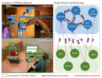
With different categories and granularity across domains, transferring relevant information and reasoning among objects can help to make a correct identification. An example of the necessity of transferring relevant information between mutliple datasets and domains can be found in Figure 1.

The most widely-used and straightforward solutions to universal detection would be to consider it as a multi-task learning problem, and integrate multiple branches upon one shared backbone network (?; ?; ?; ?; ? ?; ?; ?; ?; ?). However, they overlook the crucial semantic correlations between multiple domains and regions, such as categories hierarchy, visual similarity, and linguistic relationship since feature-level information sharing can only help to extract a more robust feature. Recently, some works explore visual reasoning and try to combine different information or interactions between objects in one image (?; ?; ?; ? ?; ?; ?; ?). For example, ? recently try to incorporate semantic relation reasoning in large-scale detection by different kinds of knowledge forms. ? introduced the Relation Networks which use an adapted attention module to allow interaction between the object’s visual features. However, they did not consider inter-domain relationship and their fully-connected relation is inefficient and noisy by incorporating redundant and distracted relationships from irrelevant objects and backgrounds.

With the advancement of geometric deep learning (?; ?; ? ?; ?; ?), using graph seems to be the most appropriate way to model relation and interaction with its flexible structure. In this paper, we present a novel universal detection system Universal-RCNN that incorporates graph learning for propagating and transferring relevant semantic information across multiple datasets to reach semantic coherency. The proposed framework first generates a global semantic pool for all domains to integrate all high-level semantic representation of categories by distilling the weights of the object classifiers. Then an Intra-Domain Reasoning Module learns a sparse regional graph to encode the regional interaction and propagates the high-level semantic graph representation from the global pool within one dataset guided by a spatial-aware Graph Convolutional Neural Network (GCN). Furthermore, an Inter-Domain Transfer Module is proposed to exploit diverse transfer dependencies across all domains and enhance the regional feature representation by attentively transferring related semantic contexts from the semantic pool in one domain to another, which bridges the gap between domains, and effectively utilize the annotations of multiple datasets. In this work, we exploit various graph transfer dependencies such as attribute/relationship knowledge, and visual/linguistic similarity. Our Universal-RCNN thus enables adaptive global reasoning and transfers over regions in multiple domains. The regional feature is greatly enhanced by abundant relevant contextual Intra/Inter-domain information and the performance on each domain is then boosted by sharing and distilling essential characteristics across domains.

Extensive experiments demonstrate the effectiveness of the proposed method and achieve the state-of-the-art results on multiple object detection benchmarks. We observe a consistent gain over multiple-branch models. In particular, Universal-RCNN achieves around 16% of mAP improvement on MSCOCO, 26% on VG, and 36% on ADE. The Universal-RCNN obtains 49.1% mAP on COCO test-dev with single-model result.

Related Work

Object Detection. Object detection is a core problem in computer vision. Most of the previous progress focus on developing new structures such as better feature fusion (?; ?; ?; ? ?; ?; ?; ?) and better receptive field to improve feature representation (?; ?; ? ?; ?; ?). However, their trained model cannot be applied directly to another related task without heavy fine-tuning.

Transfer Learning. Transfer learning (?; ?; ?; ? ?; ?; ?; ?) tries to bridge the gap between different domains or tasks to reuse the information and mitigate the burden of manual labeling. Early work (? ?) tries to learn to transfer from the ImageNet’s classification network into object detection network with fewer categories. In ?, the classifier weights are constructed by regression or a small neural network from few-shot examples or different concepts.

Multi-task Learning. Multi-task learning aims at developingRCNN can sufficiently mining the semantic correlati systems that can provide multiple outputs simultaneously for an input (?; ?; ?; ?; ? ?; ?; ?; ?; ?). For example, Mask-RCNN solves the instance segmentation problem by considering two branches: one bounding box and classification head and another dense image prediction head. ? introduced a multi-task network to handle heterogeneous annotations for unified perceptual scene parsing. However, these approaches simply create several branches separately for different tasks.

The Proposed Approach

Figure 2: An overview of our Universal-RCNN. Built on the classification layer of base detection network, global semantic pools for each domain integrate all high-level semantic representation for each category by the weights of previous classifiers. Then an Intra-Domain Reasoning Module learns a sparse regional graph to encode the regional interaction and propagates the high-level semantic graph representation from the semantic pool within one domain. Furthermore, Inter-Domain Transfer Module exploits diverse transfer dependencies across domains and enhances the regional feature representation by attentively transferring related semantic contexts from source semantic pool to the target domain, which bridges the gap between domains and utilizes the annotations of multiple datasets. Finally, the outputs of modules concatenated with region proposal features are fed into the bounding-box regression layer and classification layer to obtain better detection results. Note that this figure only illustrates how the model works within a specific pair of domains. In the whole model, we have multiple pairs of the source/target domain for the inter-domain transfer modules.

Overview

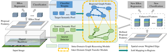
In this paper, we introduce a unified detection framework to unify all kinds of detection annotations from different domains and tackle different detection tasks in one system, that is, detecting and predicting all kinds of categories defined from multiple domains using a single network while improving the detection performance of the individual domain. This framework can be implemented on any modern dominant detection system to further improve their performance by enhancing its original image features via graph transfer learning. An overview of our model can be found in Figure 2. Specifically, we first learn and propagate compact high-level semantic representation within one domain via Intra-Domain Graph Reasoning module, and then transfer and fuse the semantic information across multiple domains to enhance the feature representation via Inter-Graph Transfer module driven by learned transfer graph or human defined hierarchical categorical structures.

Intra-Domain Reasoning Module

Given the extracted proposal visual features from the backbone, we introduce Intra-Domain Reasoning module to enhance local features for the domain $\boldsymbol{T}$, by leveraging graph reasoning with key semantic and spatial relationships. More specifically, we first create a global semantic pool to integrate high-level semantic representation for each category by collecting the weights of the original classification layer. Then a region-to-region undirected graph $\boldsymbol{G}$ : $\boldsymbol{\boldsymbol{G}_{T\rightarrow T}}=<\mathcal{N},\mathcal{\mathcal{E}}>$ for domain $\boldsymbol{T}$ is defined, where each node in $\mathcal{N}$ corresponds to a region proposals and each edge $e_{i,j}\in\mathcal{E}$ encodes relationship between two nodes. An interpretable sparse adjacency matrix is learned from the visual feature which only retains the most relevant connections for recognition of the objects. Then semantic representations over the global semantic pool are mapped to each region and propagated with a learned structure of $\boldsymbol{\boldsymbol{G}_{T\rightarrow T}}$. Finally, the proposal features are enhanced and concatenated with the original features to obtain better detection results.

Learning Graph $\boldsymbol{\boldsymbol{\boldsymbol{G}_{T\rightarrow T}}}$

We seek to learn the $\mathcal{\mathcal{E}}_{T}\in\mathbf{\mathbb{R}}^{N_{r}\times N_{r}}$ in $\boldsymbol{\boldsymbol{\boldsymbol{G}_{T\rightarrow T}}}$ thus the proposal node neighborhoods can be determined. We aim to produce a graphical representation of the relationship (e.g. attribute similarities and interactions) between proposal regions which is relevant to the object detection. Given the regional visual features $\mathbf{f}=\{\boldsymbol{f}_{i}\}_{i=1}^{N_{r}},f_{i}\in\mathbf{\mathbb{R}}^{D}$ of $D$ dimension extracted from the backbone network, we first transform $\mathbf{f}$ to a latent space $\mathbf{Z}$ by linear transformation denoted by $z_{i}=\phi(\mathbf{f}),i=1,2,...,N_{r}$, where $z_{i}\in\mathbf{\mathbb{R}}^{L}$, $L$ is the dimension of the latent space and $\phi(.)$ is a linear function. Let $\mathbf{Z}\in\mathbf{\mathbb{R}}^{N_{r}\times L}$ be the collection of normalized $\{z_{i}\}_{i=1}^{N_{r}},z_{i}\in\mathbf{\mathbb{R}}^{L}$, the adjacency matrix for $\boldsymbol{\boldsymbol{\boldsymbol{G}_{T\rightarrow T}}}$ with self loops can be calculated as $\mathcal{\mathcal{E}}=\mathbf{Z}\mathbf{Z}^{T}$, so that $e_{i,j}=\frac{z_{i}z_{j}^{T}}{\left\|z_{i}z_{j}^{T}\right\|}$, where $\left\|.\right\|$ is the L2-norm.

To determine the neighborhoods of each node, using a fully connected $\mathcal{E}$ directly will establish relationship between backgrounds(negative) samples which will lead to redundant edges and greater computation cost. In this paper, we consider a sparse graph. For each region proposal $i$, we only retain the top $t$ largest values of each row of $\mathcal{E}$, that is: $\textrm{Neighbour}(\textrm{Node }i)=\textrm{Top-t}_{j=1,..,N_{r}}(e_{i,j})$. This sparsity constraint ensures a spare graph structure focusing on the most relevant relationship for recognition of the objects.

Feature Enhanced via Intra-Domain Graph Reasoning.

Most recent existing works (?; ?; ? ?; ?; ?) propagate visual features locally among regions in the image and the information is only from those categories appearing in the image. This limits the performance of graph reasoning because of poor or distracted feature representations. Instead, we create a global semantic pool $\mathbf{P_{T}}$ to store high-level semantic representations for all categories. In some works (?; ?; ? ?; ?; ?) in zero/few-shot problem, they try to train a model to fit the weights of the classifier of an unseen/unfamiliar category and the weights of the classifier for each category can be regarded as containing high-level semantic information. Formally, let $\mathbf{P_{T}\in\mathbf{\mathbb{R}}}^{C_{T}\times(D+1)}$ denote the weights and the bias of the previous classifier for all the $C_{T}$ categories in the domain $\boldsymbol{T}$. The global semantic pool $\mathbf{P_{T}}$ is extracted from the previous classification layer in the bbox head of the detection network and can be updated in each iteration during training.

Since our graph $\boldsymbol{G}$ is a region-to-region graph, we first need to map the category semantic embedding $p_{T}\in\mathbf{P_{T}}$ to the regional representations of nodes $x_{i}\in\boldsymbol{X}$ . In this paper, we use a soft-mapping which computes the mapping weights $m_{p_{T}\rightarrow x_{i}}\in\mathbf{M_{T}}$ as $m_{p_{T}\rightarrow x_{i}}=\frac{\exp(s_{ij})}{\sum_{j}\exp(s_{ij})},$ where $s_{ij}$ is the classification score for the region $i$ towards category $j$ from the previous classification layer of the detector. Thus the regional representations of the nodes $\boldsymbol{X}\in\mathbf{\mathbb{R}}^{N_{r}\times(D+1)}$ can be computed as a matrix multiplication: $\boldsymbol{X}=\mathbf{M_{T}}\mathbf{P_{T}},$ where $\mathbf{M_{T}}\in\mathbf{\mathbb{R}}^{N_{r}\times C_{T}}$ is the soft-mapping matrix.

Given the node representation $x_{j}\in\boldsymbol{X}$ and the learned graph $\boldsymbol{\boldsymbol{\boldsymbol{G}_{T\rightarrow T}}}$, it is natural to use a GCN for modeling the relation and interaction. We thus define a patch operator for the GCN as follows:

$$\mathrm{f}_{k}^{\prime}(i)=\sum_{j\in\textrm{Neighbour}(i)}w_{k}(g_{ij})x_{j}e_{ij},$$ (1)

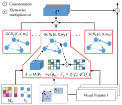
where $\textrm{Neighbour}(i)$ denotes the neighborhood of node $i$ and $e_{ij}$ is the normalized adjacency element of $\mathcal{\mathcal{E}}$. To capture the pairwise spatial information between proposals, we further add $K$ spatial weight terms $w_{k}(g_{ij})$ which are calculated by a nonlinear transformation function $w_{k}(.)$ encoding the spatial information of regions. $g_{ij}$ is a four dimensional relative geometry feature between proposal $i$ and proposal $j$: $(\log\frac{\left|x_{i}-x_{j}\right|}{w_{i}},\log\frac{\left|x_{i}-x_{j}\right|}{h_{i}},\log\frac{w_{i}}{w_{j}},\log\frac{h_{i}}{h_{j}})$, where $w_{i}$ and $h_{i}$ denotes the width and height of the region. We consider $K$ set of $w_{k}(.)$ to encode different kinds of spatial interactions. Flowchart of the graph reasoning can be found in Figure 3.

Then $\mathrm{f}^{\prime}_{k}(i)$ for each node goes through a linear transformation $\boldsymbol{L}\in\mathbf{\mathbb{R}}^{E\times(D+1)}$and is concatenated together: $\mathbf{f}^{\prime}=[L(\mathrm{f}_{k}^{\prime}(i))]$, and $KE$ is the dimension of the output enhanced feature for each region. Finally, the $\mathbf{f}^{\prime}$ for each region is concatenated to the original region features $\mathbf{f}$ to improve both classification and localization. Note that the $\mathbf{f}^{\prime}$ is a distilled information across the categories with connected edges such as similar attributes or relations. Thus, sharing the common features between categories can help to improve the feature representation by adding and discovering adaptive contexts from the global semantic pool.

Figure 3: Flowchart of our graph reasoning and transfer in Equation (1). The global semantic pool $\mathbf{P_{T}}$ is soft-mapped to the regional nodes by $\boldsymbol{X}=\mathbf{M_{T}}\mathbf{P_{T}}$. The graph edge $\mathcal{E}$ and spatial weight terms $w_{k}(g_{ij})$ are calculated from $\mathbf{f}$ and spatial information between proposal $i$ and proposal $j$. Then graph conv $GCN_{k}(.)$ is performed on the nodes $\boldsymbol{X}$ according to the graph edge $\mathcal{E}$ and $w_{k}$. Final enhanced feature $\mathbf{f}^{\prime}$ is a concatenation of all the GCN outputs. For inter-domain transfer module, the idea is similar except the input graph edge: $\mathcal{\mathcal{E}}_{S\rightarrow T}$ and the nodes: $\boldsymbol{Y}=\mathbf{M}_{\mathbf{S}}\mathbf{P_{S}}$ which are transferred from source semantic pool.

Inter-Domain Transfer Module

To effectively distill relevant information from datasets with different annotations, we introduce Inter-Domain Transfer Module to bridge the gap between different domains. This module can be applied for multiple source domains as long as they have semantic correlation. More specifically, for each pair of domains, we implement an inter-domain transfer module from source domain $\boldsymbol{S}$ to target domain $\boldsymbol{T}$. Given an image, the RPN head proposes a set of region proposals, some of which may contain objects defined in other source domains that have some relationships with objects defined in target domain $\boldsymbol{T}$. We will first extract region proposals semantic features of a certain source domain $\boldsymbol{S}$ according to the global semantic $\mathbf{P_{S}}$ pool of $\boldsymbol{S}$. Then these semantic features are transferred to the target domain $\boldsymbol{T}$ by the GCN with the predefined transfer graph $\boldsymbol{\boldsymbol{G}_{S\rightarrow T}}$ between the domain $\boldsymbol{S}$ and $\boldsymbol{T}$. Finally, the proposal features are concatenated by the information of the source domain for better prediction.

%	Method	AP	AP50	AP75	APS	APM	APL	AR1	AR10	AR100	ARS	ARM	ARL
MSCOCO	FPN (? ?)	38.6	60.4	41.8	22.3	43.2	49.8	31.8	50.5	53.2	33.9	58.0	67.1
	Multi Branches	39.9	61.5	43.4	23.5	44.9	51.4	32.7	52.4	55.2	36.3	60.3	68.3
	Universal-RCNN	44.7+6.1	65.1+4.7	49.1+7.3	26.6+4.3	49.1+5.9	58.6+8.8	35.6+3.8	56.6+6.1	59.5+6.3	39.4+5.5	64.3+6.3	75.1+8.0
VG	FPN (? ?)	7.0	12.3	7.0	3.9	7.6	10.2	14.0	19.1	19.3	10.5	19.4	22.5
	Multi Branches	7.1	12.3	7.2	4.1	7.6	10.3	13.8	19.0	19.2	10.9	19.0	22.2
	Universal-RCNN	8.8+1.8	14.2+1.9	9.3+2.3	5.0+1.1	9.4+1.8	13.3+3.1	17.5+3.5	23.7+4.6	24.0+4.7	13.4+2.9	23.3+3.9	28.8+6.3
ADE	FPN (? ?)	11.3	19.6	11.7	6.9	11.8	17.6	12.8	19.5	20.1	12.6	21.4	28.1
	Multi Branches	12.2	19.9	12.8	7.2	12.0	19.6	13.3	20.2	20.8	13.3	22.2	29.4
	Universal-RCNN	15.4+4.1	24.2+4.6	16.7+5.0	9.4+2.5	15.5+3.7	24.3+6.7	17.4+4.6	26.1+6.6	26.7+6.6	17.3+4.7	28.3+6.9	37.1+9.0

Table 1: Main results on MSCOCO(minival), VG, and ADE. “Universal-RCNN” is our full model trained on all the three domains via graph transfer and reasoning. The backbones of all the models are ResNet-101.

Construct $\boldsymbol{\boldsymbol{G}_{S\rightarrow T}}$

For different detection task with diverse categories, the attribute similarities, relationships or hierarchical correlations among them can be exploited. For example, person label in a COCO dataset contains head, arm, and leg in VG domain, and the person label can also be composed of more fine-grained categories (e.g., man, woman, boy and girl) in ADE dataset. Also, there may further exists some location and co-occurrence relationship such as “road & car”, “street & truck” and “handbag & arm”. Thus, to transfer information from source domain to target domain, we define a transfer graph $\boldsymbol{\boldsymbol{G}_{S\rightarrow T}}$, where $t_{c_{i}c_{j}}\in$$\boldsymbol{\boldsymbol{G}_{S\rightarrow T}}$ and $c_{i}$, $c_{j}$ denote the categories in source domain and target domain respectively.

In this paper we further try different methods to construct graph to explore various graph transfer dependencies between different label sets. Thus we consider and compare four schemes for $\boldsymbol{\boldsymbol{G}_{S\rightarrow T}}$ including learning the graph from feature, handcrafted attribute/relationship, and word embedding similarity.

Handcrafted Attribute. Following ?, we consider a similar way to construct a handcrafted attribute $\boldsymbol{\boldsymbol{G}_{S\rightarrow T}}$. Let us consider $K$ attributes such as colors, size, materials, and status, we obtain a $(C_{S}+C_{T})\times K$ frequency distribution table for each class-attribute pair. Then the pairwise Jensen–Shannon (JS) divergence between probability distributions $P_{c_{i}}$ and $P_{c_{j}}$ of two categories $i$ and $j$ from source/target domain can be measured as the edge weights of two classes: $t_{c_{i}c_{j}}=JS(P_{c_{i}}||P_{c_{j}})$, where JS divergence measures the similarity between two distributions.

Handcrafted Relationship. We may consider the pairwise relationship between classes, such as location relationship (e.g. along, on), the “subject-verb-object” relationship (e.g. eat, wear) or co-occurrence relationship. We can calculate frequent statistics $f_{ij}$ from the occurrence among all source-target categories pairs from additional linguistic information or through counting from images. The symmetric transformation and row normalization are performed on edge weights: $t_{c_{i}c_{j}}=\frac{f_{ij}}{\sqrt{d_{ii}d_{jj}}}$, where $d_{ii}=\sum_{j}f_{ij}$.

Word Embedding Similarity. We further explore the linguistic knowledge to construct the $\boldsymbol{\boldsymbol{G}_{S\rightarrow T}}$ besides the visual information. We use the word2vec model ? to map the semantic word of categories to a word embedding vector. Then we compute the similarity between the names of the categories in source domain and target domain: $t_{c_{i}c_{j}}=\frac{\exp(cos(w_{i},w_{j}))}{\sum_{j}\exp(cos(w_{i},w_{j}))}$, where $cos(w_{i},w_{j})$ is the cosine similarity between the word embedding vectors of the $i$th source category and $j$th target category.

Learning the Graph from Features. This scheme is almost the same as the one used in the Intra-Domain Reasoning Module. The visual feature is transformed to the latent space $z$. Edge $\mathcal{\mathcal{E}}_{S\rightarrow T}$ between the source and target domain can be calculated by $\frac{z_{i}z_{j}^{T}}{\left\|z_{i}z_{j}^{T}\right\|}$.

Feature Enhanced via Inter-Domain Transfer

After creating a global semantic pool $\mathbf{P_{S}}$ for all the $C_{S}$ categories, it is then natural to transfer high level semantic information from the source domain $\mathbf{P_{S}\in\mathbf{\mathbb{R}}}^{C_{S}\times(D+1)}$ to the target domain by the transfer graph $\boldsymbol{\boldsymbol{G}_{S\rightarrow T}}$$\mathbf{\in\mathbf{\mathbb{R}}}^{C_{S}\times C_{T}}$. Since the nodes are proposal regions, a $N_{r}\times N_{r}$ adjacent matrix $\mathcal{\mathcal{E}}_{S\rightarrow T}$ between regions can be obtained by a matrix multiplication: $\mathcal{\mathcal{E}}_{S\rightarrow T}=\mathbf{M}_{\mathbf{S}}\boldsymbol{G}_{S\rightarrow T}\mathbf{M_{T}}^{T}$ where $\mathbf{M}_{\mathbf{S}}\mathbf{\in\mathbf{\mathbb{R}}}^{N_{r}\times C_{S}}$ which is created similar to the soft-mapping by the classification score for the region towards the source categories in Section Feature Enhanced via Intra-Domain Graph Reasoning.. Then we can also obtain regional representations of nodes $y_{i}\in\boldsymbol{Y}$ from the relevant information from source domain by $\boldsymbol{Y}=\mathbf{M}_{\mathbf{S}}\mathbf{P_{S}}$.

Finally, given the node representation $y_{i}\in\boldsymbol{Y}$ and the adjacent matrix $\mathcal{\mathcal{E}}_{S\rightarrow T}\mathbf{\in\mathbf{\mathbb{R}}^{N_{r}\times N_{r}}}$, we can also use weighted GCN as Feature Enhanced via Intra-Domain Graph Reasoning. to propagate the semantic representations from the source domain to the target region nodes. Finally, the output of the GCN $\mathbf{f}_{s}^{\prime}$ is concatenated to the original visual features $\mathbf{f}$ for better classification and bounding box regression. Note that $\mathbf{f}_{s}^{\prime}$ serves as supplementary information since the relevant prediction in the source domain is transferred to each region to help better recognize the item.

Experiments

Eval	Methods	Train with	mAP	Eval	Methods	Train with	mAP
MSCOCO	FPN	-	38.6	VG	FPN	-	7.0
	Multi-Branches	VG	39.8		Multi-Branches	COCO	7.0
	Fine-tuning	VG	39.2		Fine-tuning	COCO	7.4
	Overlap Labels	VG	38.7		Universal-RCNN	COCO	8.2
	Pseudo Labels	VG	38.7		FPN	-	7.0
	Universal-RCNN	VG	43.5		Multi-Branches	ADE	7.0
	Multi-Branches	ADE	38.8		Fine-tuning	ADE	7.3
	Fine-tuning	ADE	38.6		Universal-RCNN	ADE	8.0
	Universal-RCNN	ADE	41.5	ADE	FPN	-	11.3
ADE	Multi-Branches	VG	12.3		Multi-Branches	COCO	11.4
	Fine-tuning	VG	12.8		Fine-tuning	COCO	11.9
	Universal-RCNN	VG	14.6		Universal-RCNN	COCO	12.9

Table 2: Results of mAP with models trained based on two domains. “Universal-RCNN” is our full model trained on two domains via graph transfer and reasoning. The backbones are ResNet-101.

Intra-Domain	Inter-Domain Trasfer				AP	AP50	AP75	APS	APM	APL
Reasoning	Attribute	Relation	Embed	Learn
					38.6	60.4	41.8	22.3	43.2	49.8
$\checked$					41.4	60.9	46.0	22.9	46.1	55.2
$\checked$	$\checked$				43.0	62.8	47.3	25.0	47.6	56.3
$\checked$		$\checked$			43.2	63.0	47.3	25.4	47.5	56.8
$\checked$			$\checked$		42.7	62.7	47.4	24.9	47.4	56.3
				$\checked$	41.9	60.9	46.1	23.5	46.2	55.8
$\checked$				$\checked$	43.5	63.5	47.7	25.8	47.8	57.0

Table 3: Ablation study on MSCOCO(minival) with models trained based on VG and MSCOCO domains. We consider four schemes to construct the transfer dependencies including handcrafted attribute(“Attribute”), relationship(“Relation”), word embedding similarity(“Embed”) and learning the graph from features(“Learn”). The backbones of all the models are ResNet-101.

Datasets and Evaluations. We evaluate the performance of our Universal-RCNN on three object detection domains with different annotations of categories: MSCOCO 2017 (? ?), Visual Genome(VG) (? ?), and ADE (? ?). MSCOCO is a common object detection dataset with 80 object classes, which contains 118K training images, 5K validation images (denoted as minival) and 20K unannotated testing images (denoted as test-dev) as common practice. VG and ADE are two large-scale object detection benchmarks with thousands of object classes. For VG, we use the synsets (? ?) instead of the raw names of the categories due to inconsistent label annotations. We use 88K images for training and 5K images for testing with 1000 most frequent classes, following ?; ?. For ADE, we consider 445 classes and use 20K images for training and 1K images for testing, following ?; ?. Since ADE is a segmentation dataset, we convert segmentation masks to bounding boxes for all instances. For all the evaluation, we use the standard COCO metrics including mean Average Precision (mAP) and Average Recall (AR).

Implementation Details. The proposed Universal-RCNN is a single network and trained in an end-to-end style. All tasks for multiple domains share a backbone for intermediate image feature extraction while having separated heads and transfer modules for multi-domain object feature learning. We use the popular FPN as our baseline detector and implement Universal-RCNN based on it. ResNet-101 (? ?) pretrained on ImageNet is used as the shared backbone network. The hyper-parameters in training mostly follow ?. During both training and testing, we resize the input image such that the shorter side has 800 pixels. RPN and bbox-head are applied to all levels in the feature pyramid. The total number of proposed regions after NMS is $N_{r}=512$. In the bbox-head, 2 shared FC layer is used for proposal visual feature extraction and the output is a 1024-d vector feed into the bbox regression and class-agnostic classification layer following FPN.

For the Intra-Domain graph reasoning and Inter-Domain transfer module, we use the previous 2 shared FC layer for re-extracting visual features $\mathbf{f}$ of region proposals. In the graph learner module, we use a linear transformation layer of size $256$ to learns the latent representation $\mathbf{Z}$ ($L=256$) and most $t=32$ relevant nodes are retained. The global semantic pools are created for each domain by copying the weights of the classification layers of different domains. For the spatial-aware GCN, we use two weighted graph convolutional layers with dimensions of $256$ and $128$ respectively so that the output size of the module for each region is $128$. Each GCN consists of $K=8$ spatial weight terms forming a multi-head graph attention layer (? ?). All experiments are conducted on a single server with 8 Tesla V100 GPUs by using the Pytorch framework. For training, SGD with weight decay of 0.0001 and momentum of 0.9 is adopted to optimize all models. The batch size is set to be 16 with 2 images on each GPU. The initial learning rate is 0.02, reduce twice (x0.1) during the training process. We train 12 epochs for all models in an end-to-end manner. We follow ? to prepare handcrafted Attribute/Relationship matrix with the help of the annotations in the VG dataset.

# training	Method	AP	AP50	AP75	APS	APM	APL
50%	FPN w Finetune	36.3	57.3	39.3	20.6	40.3	47.4
MSCOCO	Multi Branches	37.6	59.0	40.8	21.8	42.6	48.4
Data	Universal-RCNN	42.0	62.1	46.3	24.4	46.3	56.4
80%	FPN w Finetune	38.3	59.4	41.8	21.8	42.6	50.0
MSCOCO	Multi Branches	39.2	60.5	42.7	23.5	44.0	50.7
Data	Universal-RCNN	42.9	63.1	46.8	25.1	47.0	56.5
100%	FPN w Finetune	39.2	60.5	42.5	22.8	43.8	50.7
MSCOCO	Multi Branches	39.8	61.2	43.2	23.1	44.3	51.1
Data	Universal-RCNN	43.5	63.5	47.7	25.8	47.8	57.0

Table 4: Training with less data on MSCOCO(minival) with models trained based on VG and MSCOCO domains. We only use a portion of MSCOCO data to train the models. “FPN w Finetune” is the FPN model first trained on VG, then fintuned on MSCOCO. “FPN w Multi Branches” is the method FPN with two branches.

Comparison with state-of-the-art domain transfer baselines. To show the effecitveness of our method in transfering relevant information across multiple domains, we compare the overall performance of Universal-RCNN with several state-of-the-art domain transfer baselines including a) training an unified model on all datasets with separate RPN and bbox heads for each domain stacked on a shared backbone (Multiple Branches); b) pretraining on source dataset, fine-tuning on target dataset (Fine-tuning); c) training based on the overlap labels (Overlap Labels); d) using a fully trained model from target dataset and generate pseudo-labels on source images and train again (Pseudo-labels). The comparison results are reported on MSCOCO, VG and ADE in Table 1 and Table 2.

Table 1 shows the results of our Universal R-CNN that exploits the semantic correlations between all three datasets. We only compare our Universal R-CNN with Multiple Branches method under this setting since b), c), d) can only be used on two datasets. As can be seen, the Universal-RCNN significantly outperforms Multiple Branches method in terms of precision (1.7% to 4.8%) and recall (4.7% to 6.6%), which indicates the superiority of explicitely extracting the semantic correlatons across domains within our Universal-RCNN than implicitly learning feature-level interactions between domains within multi-task learning.

Table 2 shows the experiment results of training on each pair of domains. It can be found that our method consistently surpasses the above-mentioned domain transfer methods by a large margin through graph reasoning and transfer. Both Multiple Branches method and Fine-tuning method cannot improve detection performance much, which demonstrates the implicit way to utilize semantic information across multiple domains is ineffective. Since VG domain nearly contains all class annotations of COCO domain (79 classes out of total 80 classes), we test Overlap Labels method and Pseudo Labels method on COCO, the results show that both of them only obtain negligible 0.1% AP improvement. The reason is that the classes of VG domain have many fine-grained objects while the classes of COCO domain only have some specific objects. Table 2 also shows that transferring information from VG to COCO or ADE can achieve better detection performance, this is because that VG annotations contains a huge number of classes and many of them overlap with that of COCO and ADE. Overall, our Universal-RCNN can sufficiently mining the semantic correlations across all three domains and significantly boost the detection performance on each target domain.

Ablative Analysis. Table 3 shows the ablative analysis of our method trained based on VG and MSCOCO domains. Our Intra-domain reasoning is effective and acquires 2.8% improvements compared with the basic network on MSCOCO. For the Inter-domain transfer module, it can be found that adding the transfer module alone can boost the performance by 3.3% which demonstrates the importance of graph transfer across domains. Combining these two modules can further improve the performance by 1.6%, which demonstrates the effectiveness of the proposed Universal-RCNN in fully exploiting semantic correlations across multiple domains. We further compare four schemes to construct the transfer dependencies including handcrafted attribute, relationship, word embedding similarity and learning the graph from feature. Learning the graph from features performs better than other methods. Thus, we choose learning the graph from feature for the final model.

Training with Less Data. Since bounding box annotation is expensive, we are curious about how our Universal-RCNN performs with less training data. Table 4 shows the performance on MSCOCO with models trained based on VG and MSCOCO(less data). “FPN w Finetune” is the FPN model first trained on VG, then fintunedg on MSCOCO with less data. The Universal-RCNN is better than baseline methods with a large margin in all scenarios. Moreover, it can be found that Universal-RCNN trained on half of the data (42% mAP) outperforms FPN trained on full data (39.2% mAP). This superior performance confirms the effectiveness of our method that seamlessly bridges the gap between domains and fully utilizes data annotations. Thus, our method can be quickly adapted to new dataset with less annotation by borrowing information from other domains.

%	Method	AP	AP50	AP75
MSCOCO	SIN (? ?)	23.2	44.5	22.0
	Relation Network (? ?)	38.9	60.5	43.3
	HKRM (? ?)	37.8	58.0	41.3
	Ours w Intra-Domain	41.4	60.9	46.0
VG	HKRM (? ?)	7.8	13.4	8.1
	Ours w Intra-Domain	7.9	13.7	8.3
ADE	HKRM (? ?)	10.3	18.0	10.4
	Ours w Intra-Domain	14.0	23.1	14.9

Table 5: Comparison between intra-domain semantic correlation methods. The backbone are ResNet-101.

Comparison with semantic correlation works within one domain. There have been many works that use graph based models for additional reasoning over bounding boxes, we compare our intra-domain graph reasoning method with those intra-domain semantic correlation works in this section. We train FPN with our intra-domain module using one dataset and report the results in Table 5. It can be found that our Intra-Domain graph reasoning module is superior to multiple competing methods. It should be noted that previous works (?; ?; ? ?; ?; ?) use fully connected graphs to build object-object relationships, our method instead learn a sparse spatial-aware graph structure to perform graph inference, which can reduce lots of redundant relationships and improve the detection performance significantly. Furthermore, compare to the implicit knowledge module in ?, our method uses global semantic pool to construct bbox features and use a GCN to aggregate information.

%	Method	backbone	test-val
			AP	AP50	AP75	APS	APM	APL
MSCOCO	DetNet	DetNet-59	35.1	57.3	37.2	22.3	40.8	39.9
	DetNet w MB	DetNet-59	36.8	59.0	39.3	22.6	42.3	42.3
	DetNet w ours	DetNet-59	40.1	61.8	43.2	24.7	46.5	46.5
	HKRM	ResNet-101	40.1	61.2	44.8	23.8	43.7	51.2
	HKRM w MB	ResNet-101	41.6	62.9	45.5	24.3	45.2	52.8
	HKRM w ours	ResNet-101	43.7	63.5	47.3	24.8	46.5	55.4
	Mask-RCNN	ResNet-101	39.7	61.6	43.3	23.1	43.3	49.7
	Mask-RCNN w MB	ResNet-101	41.0	62.2	45.0	24.2	44.9	51.0
	Mask-RCNN w ours	ResNet-101	45.1	65.2	49.3	26.1	48.6	57.3
	FPN	ResNet-101	38.9	61.0	42.3	22.3	42.3	48.5
	FPN w MB	ResNet-101	40.1	61.7	43.6	23.2	43.8	49.7
	FPN w ours	ResNet-101	44.4	64.9	48.5	25.3	47.8	56.7
	FPN w ours *	ResNext-101	49.1	69.3	54.2	30.4	52.7	61.7

Table 6: Methods trained on multiple datasets(COCO, VG, ADE) and eval on COCO. “MB” is model with Multi Branches. * is the model adding multi-scale training and testing with Soft-NMS

Generalization Capacity. To validate the generalization capability of the Universal-RCNN, we further implement our method upon more recent detection methods such as DetNet (? ?), HKRM (? ?) amd Mask-RCNN (? ?) and compair. The results are reported on COCO in Table 6. Table 6 shows that Universal-RCNN consistently boost the performance by 4~6 points in terms of AP, which suggestes that the Universal-RCNN is widely applicable across different detection baselines. We futher add some bells and whistles to test the upper limit of the Universal-RCNN (? ?). Specifically, we utilize ResNext-101 as the backbone and apply multi-scale training, multi-scale testing and Soft-NMS. Finally, the Universal-RCNN obtains 49.1 mAP on COCO test-dev with single-model result.

Conclusion

In this work, we proposed a new universal object detector (Universal-RCNN) to alleviate the categories discrepancy and fully utilize the data annotation. Our method can be easily plugged into any existing detection pipeline via Transferable Graph R-CNN with multiple domains for endowing its ability to global reasoning and transferring. Extensive experiments demonstrate the effectiveness of the proposed method and achieve the state-of-the-art results on multiple object detection benchmarks.

References

- [2014] Almazán, J.; Gordo, A.; Fornés, A.; and Valveny, E. 2014. Word spotting and recognition with embedded attributes. IEEE transactions on pattern analysis and machine intelligence 36(12):2552–2566.
- [2017] Bronstein, M. M.; Bruna, J.; LeCun, Y.; Szlam, A.; and Vandergheynst, P. 2017. Geometric deep learning: going beyond euclidean data. IEEE Signal Processing Magazine 34(4):18–42.
- [2017] Chen, X., and Gupta, A. 2017. Spatial memory for context reasoning in object detection. In ICCV.
- [2018] Chen, X.; Li, L.-J.; Fei-Fei, L.; and Gupta, A. 2018. Iterative visual reasoning beyond convolutions. In CVPR.
- [2018] Cui, Y.; Song, Y.; Sun, C.; Howard, A.; and Belongie, S. 2018. Large scale fine-grained categorization and domain-specific transfer learning. In CVPR.
- [2016] Dai, J.; He, K.; and Sun, J. 2016. Instance-aware semantic segmentation via multi-task network cascades. In CVPR.
- [2010] Everingham, M.; Van Gool, L.; Williams, C. K. I.; Winn, J.; and Zisserman, A. 2010. The pascal visual object classes (voc) challenge. International Journal of Computer Vision 88(2):303–338.
- [2018] Gidaris, S., and Komodakis, N. 2018. Dynamic few-shot visual learning without forgetting. In CVPR.
- [2017] Gong, K.; Liang, X.; Zhang, D.; Shen, X.; and Lin, L. 2017. Look into person: Self-supervised structure-sensitive learning and a new benchmark for human parsing. In CVPR.
- [2018] Gong, C.; He, D.; Tan, X.; Qin, T.; Wang, L.; and Liu, T.-Y. 2018. Frage: Frequency-agnostic word representation. In NIPS.
- [2016] He, K.; Zhang, X.; Ren, S.; and Sun, J. 2016. Deep residual learning for image recognition. In CVPR.
- [2017] He, K.; Gkioxari, G.; Dollár, P.; and Girshick, R. 2017. Mask r-cnn. In ICCV.
- [2014] Hoffman, J.; Guadarrama, S.; Tzeng, E. S.; Hu, R.; Donahue, J.; Girshick, R.; Darrell, T.; and Saenko, K. 2014. Lsda: Large scale detection through adaptation. In NIPS.
- [2018a] Hu, H.; Gu, J.; Zhang, Z.; Dai, J.; and Wei, Y. 2018a. Relation networks for object detection. In CVPR.
- [2018b] Hu, R.; Dollár, P.; He, K.; Darrell, T.; and Girshick, R. 2018b. Learning to segment every thing. In Proceedings of the IEEE Conference on Computer Vision and Pattern Recognition, 4233–4241.
- [2018] Jiang, C.; Xu, H.; Liang, X.; and Lin, L. 2018. Hybrid knowledge routed modules for large-scale object detection. In NIPS.
- [2018] Kendall, A.; Gal, Y.; and Cipolla, R. 2018. Multi-task learning using uncertainty to weigh losses for scene geometry and semantics. In CVPR.
- [2018] Kirillov, A.; He, K.; Girshick, R.; Rother, C.; and Dollár, P. 2018. Panoptic segmentation. arXiv preprint arXiv:1801.00868.
- [2016] Krishna, R.; Zhu, Y.; Groth, O.; Johnson, J.; Hata, K.; Kravitz, J.; Chen, S.; Kalantidis, Y.; Li, L.-J.; Shamma, D. A.; Bernstein, M.; and Fei-Fei, L. 2016. Visual genome: Connecting language and vision using crowdsourced dense image annotations. International Journal of Computer Vision.
- [2016] Li, X.; Zhao, L.; Wei, L.; Yang, M.-H.; Wu, F.; Zhuang, Y.; Ling, H.; and Wang, J. 2016. Deepsaliency: Multi-task deep neural network model for salient object detection. IEEE Transactions on Image Processing 25(8):3919–3930.
- [2018] Li, Z.; Peng, C.; Yu, G.; Zhang, X.; Deng, Y.; and Sun, J. 2018. Detnet: A backbone network for object detection. In ECCV.
- [2015] Liang, X.; Xu, C.; Shen, X.; Yang, J.; Liu, S.; Tang, J.; Lin, L.; and Yan, S. 2015. Human parsing with contextualized convolutional neural network. In CVPR.
- [2014] Lin, T.-Y.; Maire, M.; Belongie, S.; Hays, J.; Perona, P.; Ramanan, D.; Dollár, P.; and Zitnick, C. L. 2014. Microsoft coco: Common objects in context. In ECCV.
- [2017] Lin, T.-Y.; Dollár, P.; Girshick, R.; He, K.; Hariharan, B.; and Belongie, S. 2017. Feature pyramid networks for object detection. In CVPR.
- [2018a] Liu, S.; Qi, L.; Qin, H.; Shi, J.; and Jia, J. 2018a. Path aggregation network for instance segmentation. In CVPR.
- [2018b] Liu, Y.; Wang, R.; Shan, S.; and Chen, X. 2018b. Structure inference net: Object detection using scene-level context and instance-level relationships. In CVPR.
- [2017] Luo, Z.; Mishra, A.; Achkar, A.; Eichel, J.; Li, S.; and Jodoin, P.-M. 2017. Non-local deep features for salient object detection. In CVPR.
- [2017] Misra, I.; Gupta, A.; and Hebert, M. 2017. From red wine to red tomato: Composition with context. In CVPR.
- [2017] Monti, F.; Boscaini, D.; Masci, J.; Rodola, E.; Svoboda, J.; and Bronstein, M. M. 2017. Geometric deep learning on graphs and manifolds using mixture model cnns. In CVPR.
- [2018] Peng, P.; Tian, Y.; Xiang, T.; Wang, Y.; Pontil, M.; and Huang, T. 2018. Joint semantic and latent attribute modelling for cross-class transfer learning. IEEE transactions on pattern analysis and machine intelligence 40(7):1625–1638.
- [2015] Russakovsky, O.; Deng, J.; Su, H.; Krause, J.; Satheesh, S.; Ma, S.; Huang, Z.; Karpathy, A.; Khosla, A.; Bernstein, M.; et al. 2015. Imagenet large scale visual recognition challenge. International Journal of Computer Vision 115(3):211–252.
- [2017] Tsai, Y.-H. H.; Huang, L.-K.; and Salakhutdinov, R. 2017. Learning robust visual-semantic embeddings. In ICCV.
- [2017] Velickovic, P.; Cucurull, G.; Casanova, A.; Romero, A.; Lio, P.; and Bengio, Y. 2017. Graph attention networks. In ICLR.
- [2018] Wang, X.; Girshick, R.; Gupta, A.; and He, K. 2018. Non-local neural networks. In CVPR.
- [2018] Wang, X.; Ye, Y.; and Gupta, A. 2018. Zero-shot recognition via semantic embeddings and knowledge graphs. In CVPR.
- [2018] Xiao, T.; Liu, Y.; Zhou, B.; Jiang, Y.; and Sun, J. 2018. Unified perceptual parsing for scene understanding. In ECCV.
- [2019] Xiong, Y.; Liao, R.; Zhao, H.; Hu, R.; Bai, M.; Yumer, E.; and Urtasun, R. 2019. Upsnet: A unified panoptic segmentation network. arXiv preprint arXiv:1901.03784.
- [2019a] Xu, H.; Jiang, C.; Liang, X.; and Li, Z. 2019a. Spatial-aware graph relation network for large-scale object detection. In CVPR.
- [2019b] Xu, H.; Jiang, C.; Liang, X.; Lin, L.; and Li, Z. 2019b. Reasoning-rcnn: Unifying adaptive global reasoning into large-scale object detection. In CVPR.
- [2018] Yu, F.; Xian, W.; Chen, Y.; Liu, F.; Liao, M.; Madhavan, V.; and Darrell, T. 2018. Bdd100k: A diverse driving video database with scalable annotation tooling. arXiv preprint arXiv:1805.04687.
- [2018] Zamir, A. R.; Sax, A.; Shen, W.; Guibas, L. J.; Malik, J.; and Savarese, S. 2018. Taskonomy: Disentangling task transfer learning. In CVPR.
- [2017] Zhou, B.; Zhao, H.; Puig, X.; Fidler, S.; Barriuso, A.; and Torralba, A. 2017. Scene parsing through ade20k dataset. In CVPR.
- [2019] Zhu, C.; He, Y.; and Savvides, M. 2019. Feature selective anchor-free module for single-shot object detection. arXiv preprint arXiv:1903.00621.