TurboRVB: a many-body toolkit for ab initio electronic simulations by quantum Monte Carlo

Abstract

TurboRVB  is a computational package for ab initio Quantum Monte Carlo (QMC) simulations of both molecular and bulk electronic systems. The code implements two types of well established QMC algorithms: Variational Monte Carlo (VMC), and Diffusion Monte Carlo in its robust and efficient lattice regularized variant. A key feature of the code is the possibility of using strongly correlated many-body wave functions, capable of describing several materials with very high accuracy, even when standard mean-field approaches (e.g., density functional theory (DFT)) fail. The electronic wave function (WF) is obtained by applying a Jastrow factor, which takes into account dynamical correlations, to the most general mean-field ground state, written either as an antisymmetrized geminal power with spin-singlet pairing, or as a Pfaffian, including both singlet and triplet correlations. This WF can be viewed as an efficient implementation of the so-called resonating valence bond (RVB) Ansatz, first proposed by Pauling and Anderson in quantum chemistry [L. Pauling, The Nature of the Chemical Bond (Cornell University Press, 1960)] and condensed matter physics [P.W. Anderson, Mat. Res. Bull 8, 153 (1973)], respectively. The RVB ansatz implemented in TurboRVB  has a large variational freedom, including the Jastrow correlated Slater determinant as its simplest, but nontrivial case. Moreover, it has the remarkable advantage of remaining with an affordable computational cost, proportional to the one spent for the evaluation of a single Slater determinant. Therefore, its application to large systems is computationally feasible. The WF is expanded in a localized basis set. Several basis set functions are implemented, such as Gaussian, Slater, and mixed types, with no restriction on the choice of their contraction. The code implements the adjoint algorithmic differentiation that enables a very efficient evaluation of energy derivatives, comprising the ionic forces. Thus, one can perform structural optimizations and molecular dynamics in the canonical NVT ensemble at the VMC level. For the electronic part, a full WF optimization (Jastrow and antisymmetric parts together) is made possible thanks to state-of-the-art stochastic algorithms for energy minimization. In the optimization procedure, the first guess can be obtained at the mean-field level by a built-in DFT driver. The code has been efficiently parallelized by using a hybrid MPI-OpenMP protocol, that is also an ideal environment for exploiting the computational power of modern Graphics Processing Unit (GPU) accelerator.

I Introduction

The solution of the many-body Schrödinger equation, which describes the interaction between electrons and ions at the quantum mechanical level, represents a fundamental challenge in computational chemistry, condensed matter, and materials science. Since about a century, there has been a relentless theoretical and computational effort to find an accurate solution to this problem, which also features many recent interdisciplinary applications in machine learning Ramprasad et al. (2017) and materials informatics Rajan (2005). While computationally, the scaling of the problem is exponential with the number of electrons, several numerical approximate methods have been put forward in the last decades. Among them, the Density Functional Theory (DFT) method, proposed by Kohn and Sham Kohn and Sham (1965) in 1965, is one of the most successful approaches. In this framework, the original interacting 3$N$ many-body problem ($N$ being the number of electrons in a system) is mapped to a non-interacting electron system, defined by an effective mean-field potential, to be determined self-consistently Martin (2004). While DFT is an exact theory in principle, the exact form for the exchange-correlation functional, which is an essential part of the DFT mean-field potential, remains unknown. Unfortunately, the progress in generating increasingly successful approximations of this functional is rather slow Medvedev et al. (2017), partly because there is no established strategy for systematic improvementPerdew and Schmidt (2001), while maintaining an efficient scaling with the system size. The commonly adopted approximations for the exchange-correlation DFT functional have well-known limitations especially in describing weak dispersive interactions, strongly correlated materials, and extreme environments (e.g., high pressure)Burke (2012); Cohen et al. (2012).

Alternative strategies are represented by the so-called WF-based approaches popular in quantum chemistry applications Szabo and Ostlund (1982). In these methods, electronic correlations are captured either variationally or perturbatively by post-Hartree-Fock theories, such as the Møller-Plesset perturbation theory (MP) Møller and Plesset (1934), configuration interaction (CI) and Full-CI (FCI) Knowles and Handy (1984), multi-configurational self-consistent field (MCSCF) Roos et al. (1980), Coupled-Cluster theory (CC) Čížek (1966), to name a few. Among them, coupled-cluster with single, double, and perturbative triple excitations, or CCSD(T), is considered to be the gold standard in quantum chemistry as it typically provides results in good agreement with experiments, and a reasonable balance between accuracy and computational affordability (despite its cost grows as the seventh power of the number of electrons). While quantum chemistry methods have the advantage of treating electronic exchange and correlation effects in a systematically improvable fashion, they are also much more computationally demanding compared to DFT, and their applicability to large or periodic systems is often computationally prohibitive.

Another way to tackle the problem of the electron correlation and the huge dimension of a many-body WF, exponentially large in the number of electrons, is by means of stochastic approaches, in this context referenced with the widely used expression of quantum Monte Carlo (QMC) methodsFoulkes et al. (2001); Becca and Sorella (2017). Since the invention of Markov Chain Monte Carlo (MCMC) in the 1940s,Metropolis and Ulam (1949) stochastic approaches to numerical algorithms had a pervasive influence in a wide range of fields, from physics engineering to finance. In this respect, the QMC framework is qualitatively different from the deterministic one mentioned above, and it represents, therefore, an original and alternative approach for the solution of the Schrödinger equation, overcoming some of the drawbacks of DFT and the deterministic WF-based approaches of quantum chemistry. In particular, QMC does not rely on uncontrolled approximations; its accuracy can be systematically improved, the scaling with system size is good, and it is straightforwardly applicable to both isolated and periodic systems. While the scaling with the system size is comparable with standard DFT methods, the prefactor is typically much larger. However, methods based on stochastic sampling are well suited for massively parallel computing architectures, as the algorithms can sustain an almost ideal scaling with the number of cores. As a result, the feasibility and popularity of QMC are expected to increase with the foreseeable substantial improvements in high-performance computing (HPC) facilities.

TurboRVB includes two of the most popular ground-state QMC algorithms: variational Monte Carlo (VMC) and diffusion Monte Carlo (DMC) Foulkes et al. (2001). In VMC, a systematically improvable approximation for the ground state is obtained by direct minimization of the energy, evaluated by a parametrized many-body WF. In an explicitly correlated WF, the electron coordinates are not separable, and the expectation value of the Hamiltonian has to be calculated with Monte Carlo integration, hence the name. In realistic calculations, a faithful and nevertheless compact parametrization for the trial state is essential for a successful energy optimization. The first property allows an unbiased treatment of the electronic correlations across different regimes, such as bond dissociation and electronic phase transitions. The second is needed for a stable optimization of the variational parameters, which may become a too difficult task when the chosen parametrization is redundant or unnecessarily detailed. Therefore, a central effort, in the TurboRVB project, has been devoted to the development of efficient and systematic parametrizations of correlated WFs.

As we will see in the following, an accurate trial WF is also fundamental in DMC, which is the second main algorithm present in TurboRVB. DMC is an imaginary-time projection technique Becca and Sorella (2017), that, when combined with the so-called fixed-node (FN) approximation, represents a powerful route to electronic ground-state calculations. In this approximation, the nodal-surface, which is kept fixed during the projection, can be determined by an accurate variational optimization.

So far, several groups have implemented the above algorithms and established excellent QMC codes such as QMCPACK Kim et al. (2018), CASINO Needs et al. (2009), QWALK Wagner et al. (2009), CHAMP Umrigar and Filippi , and HANDE-QMCSpencer et al. (2019). We also remark that other QMC algorithms have also been developed recently, such as the auxiliary field quantum Monte Carlo (AF-QMC) Zhang et al. (1997); Motta and Zhang (2018), full-configuration interaction quantum Monte Carlo (FCI-QMC) Booth et al. (2009, 2013), coupled cluster Monte Carlo (CCMC) Thom (2010); Spencer and Thom (2016), density matrix quantum Monte Carlo (DMQMC) Blunt et al. (2014); Malone et al. (2015), model space quantum Monte Carlo (MSQMC) Ten-no (2013); Ohtsuka and Ten-no (2015); Ten-no (2017), clock quantum Monte Carlo (CQMC)McClean and Aspuru-Guzik (2015), or driven-dissipative quantum Monte Carlo (DDQMC) Nagy and Savona (2018).

A typical workflow for a QMC calculation performed with TurboRVB is shown in Fig. 1. It shall be noticed that the choice of the most suited ansatz for the WF, as well as the optimization of its parameters, is a prerequisite of both VMC and DMC evaluations. Ionic forces, if evaluated, can be used to perform QMC-based structural relaxations, Langevin molecular dynamics (MD) or path integral molecular dynamics (PIMD). Moreover, several post-processing tools are available to analyze the outcomes. The TurboRVB code is peculiar because it relies on the assumption that a complex electronic problem, though, until now, cannot be solved exactly with a black-box computer software, can be described very accurately by approriate variational wavefunctions, guided by robust physical and chemical requirements and human ingenuity. In particular TurboRVB is different from other codes in the following features: $\rm(\hskip 1.79993pti\hskip 1.79993pt)$ It employs the Resonating Valence Bond (RVB) WF, first proposed by Pauling and Anderson in quantum chemistry Pauling (1960) and condensed matter physics Anderson (1973), respectively. It includes static and dynamical correlation effects beyond the commonly used Slater determinant, while keeping the computational cost at the single-determinant level, thanks to its efficient implementation. $\rm(\hskip 0.80002ptii\hskip 0.80002pt)$ The code implements a VMC algorithm based on localized orbitals (e.g., Gaussians) and state-of-the-art optimization methods, such as the stochastic reconfiguration. Therefore, at the VMC level, one can optimize not only the amplitude of the WF (i.e., the Jastrow factor), but also the nodal surfaces (e.g., the Slater determinant). This leads to a better variational energy in general, and also improves the corresponding FN-DMC energy. $\rm(iii)$ The energy derivatives (e.g., atomic forces) are calculated very efficiently thanks to an implementation based on the Adjoint Algorithmic Differentiation (AAD). As a consequence, one can perform structural optimizations and Langevin molecular dynamics. $\rm(iv)$ The code implements the newly developed Lattice Regularized Diffusion Monte Carlo (LRDMC), a stable DMC algorithm that, very recently, has shown to have a better scaling with the atomic number $Z$, compared with standard DMC. Nakano et al. (2020)

This review is organized as follows: in Sec. II, we briefly explain the fundamental QMC algorithms implemented in TurboRVB, namely, the VMC and LRDMC; in Sec. III, we describe the RVB WF; in Sec. IV, we extend the WF to treat periodic systems; in Sec. V we introduce the DFT algorithm efficiently implemented in TurboRVB; in Sec. VI, we describe the way energy derivatives are computed (e.g., atomic forces) by means of AAD; in Sec. VII, we list the TurboRVB, steps to optimize a many-body WF; in Sec. VIII, we introduce the first and the second-order Langevin molecular dynamics implemented in TurboRVB; in Sec. IX, we summarize the typical QMC workflow from the WF generation to the final LRDMC calculation; in Sec. X, we show weak and strong scaling results of TurboRVB, measured on the Marconi/CINECA supercomputer; in Sec  XI, we list the physical properties that can be calculated by TurboRVB; in Sec. XII, we review the major TurboRVB  applications done so far; in Sec. XIII, we introduce a python-based workflow system, named Turbo-Genius.

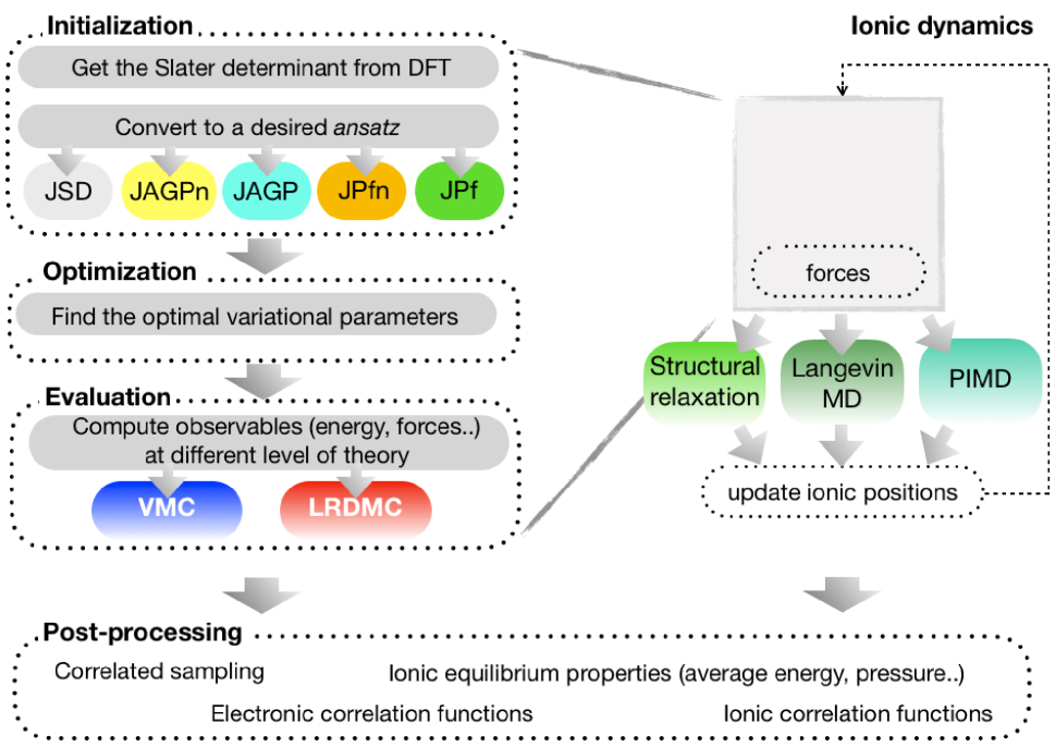
Figure 1: Schematic picture of some of the possible tools available in TurboRVB. The arrows indicate typical workflow calculations.

Table 1: Summary of the notations used in this review.

Notation	Description
${\mathbf{r}_{i}}$	$i$-th electron coordination.
${\mathbf{R}_{a}}$	$a$-th ion coordination.
${\sigma_{i}}$	spin of $i$-th electron.
${\mathbf{x}_{i}}$	$N$ set of electron coordinations including spins $\equiv$ $\left({{{\mathbf{r}}_{1}}{\sigma_{1}},{{\mathbf{r}}_{2}}{\sigma_{2}},\ldots{{\mathbf{r}}_{N}}{\sigma_{N}}}\right)_{i}$. The index $i$ referes Monte Carlo sampling index.
${\mathbf{x}}$	$N$ set of electron coordinations including spins, the same as ${\mathbf{x}_{i}}$.
$\mathbf{i}$, $\mathbf{j}$	compact notation for (${\mathbf{r}_{i}},{\sigma_{i}}$) and (${\mathbf{r}_{j}},{\sigma_{j}}$), respectively.
$\int d\mathbf{i}$	compact notation for $\sum_{\sigma_{i}}\int d\mathbf{r}_{i}.$
$a,b,I,J$	indices of atoms.
$i,j$	indices of electrons / orbitals / Monte Carlo sampling.
$\mu$, $\nu$	indices of orbitals.
$l,m$	indices of orbitals.
$M$	the number of configurations of electrons (the number of Monte Carlo sampling).
$N_{\textrm{at}}$	the number of atoms.
$N$	the number of electrons.
$N_{u}$	the number of electrons with spin up.
$N_{d}$	the number of electrons with spin down.
${{\alpha_{1}},\cdots,{\alpha_{p}}}$	variational parameters of the trial WF
$\alpha_{k}$	$k$-th variational parameter.
${\Psi}$	many-body WF ansatz. $\Psi=\Phi_{\text{AS}}\times\exp J$.
${\cal A}$	antisymmetrization operator.
$\Phi_{\text{AS}}$	antisymmetric (AS) part.
$\Phi_{\text{SD}}$	single Slater determinant (SD).
$\Phi_{\text{AGP}}$	antisymmetrized Geminal Power (AGP).
$\Phi_{\text{Pf}}$	pfaffian (Pf).
$J$	Jastrow factor, composed of $J_{1}$, $J_{2}$, and $J_{3/4}$.
${\Psi_{\text{T}}}$	many-body trial WF.
${\Psi_{\text{G}}}$	many-body guiding function.
$G$	$N\times N$ matrix with elements $G_{i,j}=g(\mathbf{i},\mathbf{j})$.
$\Phi$	$N$ $\times$ $k$ matrix with elements $\Phi_{i,k}={{\phi}_{k}}\left(\mathbf{i}\right)$.
$g\left(\mathbf{i},\mathbf{j}\right)$	pairing function between electrons $\mathbf{i}\leftrightarrow({\bf r}_{i},\sigma_{i})$ and $\mathbf{j}\leftrightarrow({\bf r}_{j},\sigma_{j})$.
$f\left({\mathbf{r}}_{i},{\mathbf{r}}_{j}\right)$	spatial part of the pairing function.
${\psi_{i}}\left({\mathbf{r}}\right)$	primitive atomic orbital for the antisymmetric part.
${{\phi}_{k}}\left({\mathbf{r}}\right)$	$k$-th molecular orbital for the antisymmetric part.
${\chi_{i}}\left({\mathbf{r}}\right)$	primitive atomic orbital for the Jastrow part.
$\mathbf{S}$	overlap matrix with elements $S_{\mu,\nu}\equiv\langle\psi_{\mu}|\psi_{\nu}\rangle$.
${f_{i}}$	general force for $i$-th variational parameter ${f_{i}}$ $\equiv$ - $\frac{{\partial E}}{{\partial{\alpha_{i}}}}$.
${{\mathbf{F}}_{a}}$	atomic force for an atom $a$, ${{\mathbf{F}}_{a}}$ $\equiv$ $-\frac{{dE}}{{d{{\mathbf{R}}_{a}}}}$.
${O_{k}}\left({{{\mathbf{x}}}}\right)$	the logarithmic derivative of a many-body WF ${O_{k}}\left({{{\mathbf{x}}}}\right)$ $\equiv$ $\frac{{\partial\ln\Psi\left({{{\mathbf{x}}}}\right)}}{{\partial{\alpha_{k}}}}$.
${\bm{\mathcal{S}}}$	variance-covariance matrix of the logarithmic derivative of a many-body WF.
${\bm{\mathcal{S}}}^{{{\text{QMC}}}}\left({\mathbf{R}}\right)$	variance-covariance matrix of QMC forces.

II Methods

TurboRVB  implements two types of well established Quantum Monte Carlo methods: Variational Monte Carlo (VMC) and Lattice Regularized Diffusion Monte Carlo (LRDMC). We summarize these methods in this section. The interested readers should also refer to the comprehensive review of QMC Foulkes et al. (2001) for details. TurboRVB  also implements an original DFT engine to generate trial WFs, which is more suitable for the VMC and LRDMC calculations, as shown in Sec. V.

II.1 Variational Monte Carlo

Starting from the variational principle, the expectation value of the energy evaluated for a given WF $\Psi$ can be written as:

$$\left\langle E\right\rangle=\frac{{\int{d{\mathbf{x}}{\Psi^{2}}\left({\mathbf{x}}\right)\cdot\hat{\mathcal{H}}\Psi\left({\mathbf{x}}\right)/\Psi\left({\mathbf{x}}\right)}}}{{\int{d{\mathbf{x}}{\Psi^{2}}\left({\mathbf{x}}\right)}}}=\int{d{\mathbf{x}}{e_{L}}\left({\mathbf{x}}\right)\pi\left({\mathbf{x}}\right)},$$ (1)

where ${\mathbf{x}}=\left({{{\mathbf{r}}_{1}}{\sigma_{1}},{{\mathbf{r}}_{2}}{\sigma_{2}},\ldots{{\mathbf{r}}_{N}}{\sigma_{N}}}\right)$ here and henceforth is a shorthand notation for the $N$ electron coordinates and their spins, whereas

$${e_{L}}\left({\mathbf{x}}\right)\equiv{\hat{\mathcal{H}}\Psi\left({\mathbf{x}}\right)\over\Psi\left({\mathbf{x}}\right)}\quad,\text{and}\quad\pi\left({\mathbf{x}}\right)\equiv{{\Psi^{2}}\left({\mathbf{x}}\right)\over\int{d{\mathbf{x^{\prime}}}{\Psi^{2}}\left({\mathbf{x^{\prime}}}\right)}},$$

are the so-called local energy and the probability of the configuration $\mathbf{x}$, respectively. This multidimensional integration can be evaluated stochastically by generating a set $\left\{{{{\mathbf{x}}_{i}}}\right\}$ according to the distribution $\pi\left({\mathbf{x}}\right)$ using the Markov chain Monte Carlo such as the (accelerated Umrigar (1993); Stedman et al. (1998)) Metropolis method, and by averaging the obtained local energies ${e_{L}}\left({{{\mathbf{x}}_{i}}}\right)$:

$${E_{{\text{VMC}}}}={\left\langle{{e_{L}}\left({\mathbf{x}}\right)}\right\rangle_{\pi\left({\mathbf{x}}\right)}}\approx\frac{1}{M}\sum\limits_{i=1}^{M}{{e_{L}}\left({{{\mathbf{x}}_{i}}}\right)},$$ (2)

which has an associated statistical error of $\sqrt{{\text{Var}[e_{L}(\mathbf{x}_{i})]/\tilde{M}}}$, where $\text{Var}[e_{L}(\mathbf{x}_{i})]$ is the variance of the sampled local energies, and $\tilde{M}$ is the sampling size $M$ divided by the autocorrelation time. This indicates that the precision of the VMC evaluation is inversely proportional to the square root of the number of samplings (i.e., of the computational cost). It worth to notice that, if $\Psi(\mathbf{x})$ is an eigenfunction of $\hat{\mathcal{H}}$, say with eigenvalue $E_{0}$, then $e_{L}(\mathbf{x})=E_{0}$ for each $\mathbf{x}$, implying that the variance of the local energy is zero and $E_{\text{VMC}}=E_{0}$ with no stochastic uncertainty. This feature is known as the zero-variance property.

The probability distribution used for the importance sampling can also differ from $\pi\left({\mathbf{x}}\right)$. Indeed, one can use an arbitrary probability distribution function $\pi^{\prime}\left({\mathbf{x}}\right)=\Psi_{\text{G}}^{2}\left({\mathbf{x}}\right)/\int{d{\mathbf{x}}\Psi_{\text{G}}^{2}\left({\mathbf{x}}\right)}$, and estimate a generic local observable $O\left({\mathbf{x}}\right)$ either by using ${{\bar{O}}_{{\text{VMC}}}}={\left\langle{O\left({\mathbf{x}}\right)}\right\rangle_{\pi\left({\mathbf{x}}\right)}}$ or:

$${{\bar{O}}_{{\text{VMC}}}}=\frac{{{{\left\langle{O\left({{\mathbf{x^{\prime}}}}\right)\mathcal{W}\left({{\mathbf{x^{\prime}}}}\right)}\right\rangle}_{\pi^{\prime}\left({{\mathbf{x^{\prime}}}}\right)}}}}{{{{\left\langle{\mathcal{W}\left({{\mathbf{x^{\prime}}}}\right)}\right\rangle}_{\pi^{\prime}\left({\mathbf{x}}\right)}}}}\approx\frac{{\sum\nolimits_{i=1}^{M^{\prime}}{O\left({{{{\mathbf{x^{\prime}}}}_{i}}}\right)\mathcal{W}\left({{{{\mathbf{x^{\prime}}}}_{i}}}\right)}}}{{\sum\nolimits_{i=1}^{M^{\prime}}{\mathcal{W}\left({{{{\mathbf{x^{\prime}}}}_{i}}}\right)}}},$$ (3)

where $\mathcal{W}\left({{{{\mathbf{x}}}}}\right)=|{\Psi}\left({\mathbf{x}}\right)/\Psi_{\text{G}}\left({\mathbf{x}}\right)|^{2}$, and the points $\mathbf{x^{\prime}}_{i}$ are distributed according to $\pi^{\prime}$. This reweighting scheme is very important when evaluating atomic forces, as discussed in Sec. VI.2. Since the evaluations of the standard deviations is nontrivial in this case, TurboRVB employs the bootstrap and jackknife methods in order to estimate the mean value and the statistical error Becca and Sorella (2017), which are also used when evaluating those of the local energy, forces, and so on. Indeed, the code outputs the history of the local energies, forces, or other properties in appropriate files (when the corresponding option is true), thus allowing the error bar estimates by simple post-processing. The user can also use the reblocking (binning) technique to remove the autocorrelation bias.Flyvbjerg and Petersen (1989)

One can optimize the WF based on the variational theorem by introducing a set of parameters $\left({{\alpha_{1}},{\alpha_{2}},\cdots,{\alpha_{p}}}\right)$ to the WF ${\Psi\left({{\mathbf{x}},\mathbf{\alpha}}\right)}$:

$${E_{{\text{VMC}}}}\left(\alpha\right)=\int{d{\mathbf{x}}{e_{L}}\left({{\mathbf{x}},\alpha}\right)\pi\left({{\mathbf{x}},\alpha}\right)}\geqslant{E_{{\text{exact}}}}.$$ (4)

However, the optimization of a many-body WF remains a difficult challenge not only because optimizing a cost function containing many parameters is a complex numerical task, due to the presence of several local minima in the energy landscape, but also because this difficult task is further complicated by the presence of statistical errors in the QMC evaluation of any quantity. Nevertheless, a great improvement in this field has been achieved when the QMC optimization techniques have made use of the explicit evaluation of energy derivatives with finite statistical errors. In particular, in TurboRVB  the adjoint algorithmic differentiation (AAD) has been implemented, by allowing the efficient calculation of generalized forces (${f_{i}}=-\frac{{\partial E}}{{\partial{\alpha_{i}}}}$) Sorella and Capriotti (2010), and very efficient optimization methods, the so-called “stochastic reconfiguration” Sorella (1998); Sorella et al. (2007) and “the linear method” Sorella (2005); Umrigar et al. (2007); Toulouse and Umrigar (2007). These methods are discussed in Sec. VII.1 and VII.2.

II.2 Lattice regularized Monte Carlo

Lattice regularized diffusion Monte Carlo (LRDMC), which was initially proposed by M. Casula et al. Casula et al. (2005a), is a projection technique that allows us to improve a variational ansatz systematically. This method is based on Green’s function Monte Carlo (GFMC) Ten Haaf et al. (1995); Calandra Buonaura and Sorella (1998); Sorella and Capriotti (2000), filtering out the ground state WF ${\left|{{\Upsilon_{0}}}\right\rangle}$ from a given trial WF $\left|{{\Psi_{\text{T}}}}\right\rangle$: since the eigenstates of the Hamiltonian have the completeness property, the trial WF can be expanded as:

$$\left|{{\Psi_{\text{T}}}}\right\rangle=\sum\limits_{n}{{a_{n}}\left|{{\Upsilon_{n}}}\right\rangle},$$ (5)

where ${a_{n}}$ is the coefficient for the $n$-th eigenvectors (${{\Upsilon_{n}}}$). Therefore, by applying ${{\mathcal{G}}^{M}}={\left({{\bm{\Lambda}}-\hat{\bm{\mathcal{H}}}}\right)^{M}}$, one can obtain

$$\begin{split}\left|{{\Upsilon_{0}}}\right\rangle&\propto\mathop{\lim}\limits_{M\to\infty}{\left({{\bm{\Lambda}}-\hat{\mathcal{H}}}\right)^{M}}\left|{{\Psi_{\text{T}}}}\right\rangle\\ &=\mathop{\lim}\limits_{M\to\infty}{\left({\lambda-{E_{0}}}\right)^{M}}\left[{{a_{0}}\left|{{\Upsilon_{0}}}\right\rangle+\sum\limits_{n\neq 0}{{{\left({\frac{{\lambda-{E_{n}}}}{{\lambda-{E_{0}}}}}\right)}^{M}}{a_{n}}\left|{{\Upsilon_{n}}}\right\rangle}}\right],\end{split}$$ (6)

where ${\bm{\Lambda}}$ is a diagonal matrix with ${{\Lambda_{x,x^{\prime}}}}=\lambda\delta_{x,x^{\prime}}$ ($\lambda$ should be sufficiently large to obtain the ground state), and ${{E_{n}}}$ is $n$-th eigenvalue of $\hat{\mathcal{H}}$. Since $\frac{{\lambda-{E_{n}}}}{{\lambda-{E_{0}}}}<1$, the projection filters out the ground state WF ${{\Upsilon_{0}}}$ from a given trial WF $\left|{{\Psi_{\text{T}}}}\right\rangle$, as long as the trial WF is not orthogonal to the true ground state (i.e., ${a_{0}}\equiv\left<\Upsilon_{0}|\Psi_{\text{T}}\right>\neq 0$). To apply the GFMC for ab initio electron calculations, the original continuous Hamiltonian is regularized by allowing electron hopping with step size $a$, in order to mimic the electronic kinetic energy. The corresponding Hamiltonian ${{\hat{\mathcal{H}}}^{a}}$ is then defined such that ${{{\hat{\mathcal{H}}}^{a}}}\to{\hat{\mathcal{H}}}$ for $a\to 0$. Namely, the kinetic part is approximated by a finite difference form:

$$\begin{split}{\Delta_{i}}f\left({{x_{i}},{y_{i}},{z_{i}}}\right)&\approx\Delta_{i}^{a}f\left({{x_{i}},{y_{i}},{z_{i}}}\right)\\ &\equiv\frac{1}{{{a^{2}}}}\left\{{\left[{f\left({{x_{i}}+a}\right)-f\left({{x_{i}}}\right)}\right]+\left[{f\left({{x_{i}}-a}\right)-f\left({{x_{i}}}\right)}\right]}\right\}\\ &\leftrightarrow{y_{i}}\leftrightarrow{z_{i}},\end{split}$$ (7)

and the potential term is modified as:

$${V^{a}}\left({\mathbf{x}}\right)=V\left({\mathbf{x}}\right)+\frac{1}{2}\left[{\frac{{\sum\nolimits_{i}{\left({\Delta_{i}^{a}-{\Delta_{i}}}\right)\Psi_{\text{G}}\left({\mathbf{x}}\right)}}}{{{\Psi_{\text{G}}}\left({\mathbf{x}}\right)}}}\right].$$ (8)

The corresponding Green’s function matrix elements are:

$${{\mathcal{G}}_{{x^{\prime},x}}}=\braket{{x^{\prime}}}{({\bm{\Lambda}}-{\bm{{\hat{\mathcal{H}}}}}^{a})}{{x}}\equiv\left({\bm{\Lambda}}-{\bm{{{\mathcal{H}}}}}^{a}\right)_{{x^{\prime},x}}$$ (9)

and the single LRDMC iteration step is given by the following equation:

$${\Psi_{n+1}}\left({x^{\prime}}\right)=\sum\limits_{x}{{{\mathcal{G}}_{x^{\prime},x}}{\Psi_{n}}\left(x\right)}.$$ (10)

The sketch of the LRDMC algorithm, a Markov chain that evolves the many-body WF according to the Eq. 10, is as follows Casula et al. (2005a): (STEP 1) Prepare a walker with configuration $x$ and weight $w$ ($w_{0}$ = 1). (STEP 2) A new configuration $x^{\prime}$ is generated by the transition probability:

$${p_{x^{\prime},x}}={{\mathcal{G}}_{x^{\prime},x}}{\rm{/}}{b_{x}},$$ (11)

where

$${b_{x}}=\sum\nolimits_{x^{\prime}}{{{\mathcal{G}}_{x^{\prime},x}}}$$ (12)

is a normalization factor. By applying the discretized Hamiltonian to a given configuration (${{\hat{\mathcal{H}}}^{a}}\ket{x}$), $(6N+1)$ configurations $\ket{x^{\prime}}$ are determined according to the probability ${p_{x^{\prime},x}}$ in Eq. 11, where $N$ is the number of electrons in the system Casula (2005). This allows the evaluation of the normalization factor ${b_{x}}$ in Eq. 12 even in a continuous model. Notice that $6N$ comes from the diffusion of each electron in two directions ($\pm a$) and the remaining $1$ stands for the starting configuration $x$ before the possible hoppings (all $N$ electrons) (i.e., $x^{\prime}=x$). (STEP 3) Finally, update the weight with ${w_{n+1}}={w_{n}}{b_{x}}$, and return to the STEP I. After a sufficiently large number of iterations (the Markov process is equilibrated), one can calculate the ground state energy ${E_{0}}$:

$${E_{0}}\approx\frac{{\left\langle{{w_{n}}{e_{L}}\left({{x_{n}}}\right)}\right\rangle}}{{\left\langle{{w_{n}}}\right\rangle}},$$ (13)

where ${\left\langle{\cdots}\right\rangle}$ denotes the statistical average over many independent samples generated by the Markov chain, and ${e_{L}}\left(x\right)$ is called the (bare) local energy that reads:

$${e_{L}}\left(x\right)=\sum\limits_{x^{\prime}}{{{\mathcal{H}}_{x^{\prime},x}}=\lambda-{b_{x}}}.$$ (14)

Indeed, the ground state energy can be calculated after many independent $n$-step calculations. A more efficient computation can be realized by using the so-called ”correcting factor” technique: after a single simulation that is much larger than the equilibration time, one can imagine starting a projection of length $p$ from each $(n-p)^{th}$ iteration. The accumulated weight for each projection is:

$${\mathcal{G}}_{n}^{p}=\prod\limits_{j=1}^{p}{{b_{n-j}}}.$$ (15)

Then, the ground state energy ${E_{0}}$ can be estimated by:

$${E_{0}}\approx\frac{{\sum\nolimits_{n}{{\mathcal{G}}_{n}^{p}{e_{L}}\left({{x_{n}}}\right)}}}{{\sum\nolimits_{n}{{\mathcal{G}}_{n}^{p}}}}.$$ (16)

This straightforward implementation of the above simple method is not suitable for realistic simulations due to fluctuations of weights, large correlation times, the sign problems, and so on. TurboRVB  implements the following state-of-art techniques for real electronic structure calculations.

If the potential term (Eq. 8) is unbounded (it is the case in ab initio calculations), the bare weight ${b_{x}}$ (Eq. 12) and the local energy ${e_{L}}\left(x\right)$ (Eq. 14) significantly fluctuate, making the numerical simulation very unstable and inefficient. To overcome this difficulty, the code employs the importance sampling scheme Becca and Sorella (2017), in which the original Green’s function is modified using the so-called guiding function ${\Psi_{\text{G}}}$ as:

$${{\tilde{\mathcal{G}}}_{x^{\prime},x}}={{\mathcal{G}}_{x^{\prime},x}}\frac{{{\Psi_{\text{G}}}\left({x^{\prime}}\right)}}{{{\Psi_{\text{G}}}\left(x\right)}},$$ (17)

and the projection is modified as:

$${\Psi_{\text{G}}}\left({x^{\prime}}\right){\Psi_{n+1}}\left({x^{\prime}}\right)=\sum\limits_{x}{{{\tilde{\mathcal{G}}}_{x^{\prime},x}}{\Psi_{\text{G}}}\left(x\right){\Psi_{n}}\left(x\right)}.$$ (18)

In practice, the guiding function is prepared by a VMC calculation. The modified Green’s function for importance sampling ${{\tilde{\mathcal{G}}}_{x^{\prime},x}}$ has the same eigenvalues as the original one, and this transformation does not change the formalism of LRDMC. The weight is updated by:

$${{\tilde{b}}_{x}}=\sum\limits_{x^{\prime}}{{{\tilde{\mathcal{G}}}_{x^{\prime},x}}},$$ (19)

and the local energy with importance sampling is:

$${{\tilde{e}}_{L}}\left(x\right)=\frac{\braket{{\Psi_{\text{G}}}{\hat{\mathcal{H}}}{x}}{missing}{missing}}{{\braket{\Psi_{\text{G}}}{x}}}=\sum\limits_{x^{\prime}}{{{\mathcal{H}}_{x^{\prime},x}}\frac{{\Psi_{\text{G}}\left({x^{\prime}}\right)}}{{\Psi_{\text{G}}\left(x\right)}}}.$$ (20)

Eq. 20 implies that if the guiding function ${\Psi_{\text{G}}}$ is an exact eigenstate of the Hamiltonian, there are no statistical fluctuations, implying the zero variance property, namely the computational efficiency to obtain a given statistical error on the energy improves with the quality of the variational WF. In this respect, it is also important to emphasize that a meaningful reduction of the statistical fluctuations is obtained by satisfying the so-called cusp conditions. As long as they are satisfied, the resulting local energy does not diverge at the coalescence points where two particles are overlapped, despite the singularity of the Coulomb potential term ($V(x)$ in Eq. 8) Casula (2005). In addition, the importance sampling maintains the electrons in a region away from the nodal surface, since the guiding function vanishes there (i.e., the RHS of Eq.17 $\to$ 0). This clearly enhances the efficiency of the sampling because the local energy diverges at the nodal surface.

The Green’s function cannot be made strictly positive for fermions; therefore, the fixed-node (FN) approximation has to be introduced Becca and Sorella (2017) in order to avoid the sign problem. Indeed, the Hamiltonian is modified using the spin-flip term ${\mathcal{V}_{{\rm{sf}}}}\left({x}\right)=\sum\limits_{x^{\prime}:{s_{x^{\prime},x}}>0}{{{\mathcal{H}}_{x^{\prime},x}}{\Psi_{\text{G}}}\left({x^{\prime}}\right)}/{\Psi_{\text{G}}}\left({x}\right)$:

$${\mathcal{H}}_{x^{\prime},x}^{\text{FN},\gamma}=\begin{cases}{{\mathcal{H}}_{x,x}}+\left({1+\gamma}\right){\mathcal{V}_{{\rm{SF}}}}\left({x}\right)\,\,\,\,{\rm{for}}\,\,\,\,x^{\prime}=x,\\ {{\mathcal{H}}_{x^{\prime},x}}\,\,\,\,\,\,\,\,\,\,\,\,\,\,\,\,\,\,\,\,\,\,\,\,\,\,\,\,\,\,\,\,\,\,\,\,\,\,\,\,{\rm{for}}\,\,\,\,x^{\prime}\neq x,{s_{x^{\prime},x}}<0,\\ -\gamma{{\mathcal{H}}_{x^{\prime},x}}\,\,\,\,\,\,\,\,\,\,\,\,\,\,\,\,\,\,\,\,\,\,\,\,\,\,\,\,\,\,\,\,\,{\rm{for}}\,\,\,\,x^{\prime}\neq x,{s_{x^{\prime},x}}>0,\end{cases}$$ (21)

where ${s_{x^{\prime},x}}={\Psi_{\text{G}}}\left({x^{\prime}}\right){{\mathcal{H}}_{x^{\prime},x}}/{\Psi_{\text{G}}}\left({x}\right)$ and $\gamma\geq 0$ is a real parameter. The use of the fixed-node Green’s function:

$$\tilde{\mathcal{G}}_{{x^{\prime},x}}^{{\text{FN}}}=\left({\bm{\Lambda}-{\mathcal{H}}^{{\text{FN}}}}\right)_{x^{\prime},x}\frac{{\Psi_{\text{G}}\left({x^{\prime}}\right)}}{{\Psi_{\text{G}}\left(x\right)}}$$ (22)

can prevent the crossing of regions where the configuration space yields a sign flip of the Green’s function; therefore, the walkers are constrained in the same nodal pockets, and avoid the sign problem.

TurboRVB  also implements the many-walker technique and the branching (denoted as reconfiguration Calandra Buonaura and Sorella (1998) in TurboRVB) scheme for a more efficient computation Becca and Sorella (2017). The code performs the branching as follows: (1) Set the new weights equal to the average of the old ones:

$${{w^{\prime}}_{\alpha,n}}=\bar{w}\equiv\frac{1}{{{N_{w}}}}\sum\limits_{\beta}{{w_{\beta,n}}}.$$ (23)

(2) Select the new walkers from the old ones with a probability that is proportional to the old walkers’ weights:

$${p_{\alpha,n}}=\frac{{{w_{\alpha,n}}}}{{\sum\limits_{\beta}{{w_{\beta,n}}}}},$$ (24)

which does not change the statistical average of weights, but suppresses the fluctuations by dropping walkers having small weights. The code performs branching (reconfiguration) after a projection time $\tau$, that can be chosen as a user input parameter. In practice, within the many-walker and branching schemes, the average weights are stored and are set to one for all walkers after each branching. The user can retrieve the accumulated weights at the end of the simulation:

$${\mathcal{G}}_{n}^{p}=\prod\limits_{j=1}^{p}{{{\bar{w}}_{n-j}}},$$ (25)

and calculate the ground state energy:

$${E_{0}}\approx\frac{{\sum\nolimits_{n}{{\mathcal{G}}_{n}^{p}{e_{L}}\left({{x_{n}}}\right)}}}{{\sum\nolimits_{n}{{\mathcal{G}}_{n}^{p}}}},$$ (26)

where ${e_{L}}\left({{x_{n}}}\right)$ is the mean local energy averaged over the walkers, which reads:

$${e_{L}}\left({{x_{n}}}\right)=\frac{{\sum\nolimits_{\alpha}{{w_{\alpha,n}}{e_{L}}\left({{x_{\alpha,n}}}\right)}}}{{\sum\nolimits_{\alpha}{{w_{\alpha,n}}}}}$$ (27)

and is evaluated just before each reconfiguration. Notice that $p$ is also an input parameter, that has to be carefully chosen by the user to allow energy convergence.

When $\lambda$ is sufficiently large, the correlation time also becomes large because the diagonal terms of the Green’s function become very close to one (i.e., a walker remains in the same configuration), which causes a very large correlation time. In TurboRVB, this difficulty is solved by considering in a different way the diagonal and non-diagonal moves. In a given interval of $M$ iterations, The non-diagonal updates are efficiently calculated using a random number according to the probability that the configuration remains in the same one (diagonal updates). This technique can be generalized to the continuous-time limit, namely, $M\to\infty$, at ${M\over\Lambda}=\tau$ fixed. In the $M\to\infty$ limit, the projection ${\left({\Lambda-\hat{\mathcal{H}}}\right)^{M}}$ is equal to the imaginary time evolution $\exp\left({-\tau\hat{\mathcal{H}}}\right)$, apart for an irrelevant constant $\Lambda^{M}$. Thus the user should specify only $\tau$ as input parameter. Indeed, the walker weight is updated by $w\to w\exp\left({-{\tau_{\xi}}{e_{L}}\left(x\right)}\right)$ and the imaginary time is updated ${\tau_{{\text{left}}}}\to{\tau_{{\text{left}}}}-{\tau_{\xi}}$ at each non-diagonal update until ${\tau_{{\text{left}}}}$ becomes 0, where ${\tau_{\xi}}=-\log\left(1-{\xi}\right)/{b_{x}}$ is a diagonal move time step determined by a uniform random number $0\leq\xi<1$. The branching (reconfiguration) is performed after each projection time of length $\tau$ that a user puts in the input file within the many walker and the branching implementation.

In practice, there are three important features in LRDMC. First, there is not a time-step error in LRDMC because the Suzuki-Trotter decomposition is not necessary, unlike the standard DMC algorithm Becca and Sorella (2017). Instead, there is a finite-size lattice error due to the discretization of the Hamiltonian ($a$). Therefore, in order to obtain an unbiased FN energy, it is important to extrapolate the LRDMC energy to the $a\to 0$ limit by using several results corresponding to different lattice spaces Casula et al. (2005a). This is then consistent with the standard DMC energy estimate (Fig. 2) obtained in the limit of an infinitely small time step. Probably one of the most important advantages of the LRDMC method is that the extrapolation to the $a\to 0$ limit is very smooth and reliable, so that unbiased FN energies are easily obtained with low order polynomial fits. Secondly, LRDMC can straightforwardly handle different length scales of a WF by introducing different mesh sizes ($a$ and $a^{\prime}$), so that electrons in the vicinity of the nuclei and those in the valence region can be appropriately diffusedCasula et al. (2005a); Nakano et al. (2020), which defines the so-called double-grid LRDMC. This scheme saves a substantial computational cost in all-electron calculations, especially for a system including large atomic number atomsNakano et al. (2020), with a typical computational cost scaling with $Z^{\sim 6}$ where $Z$ is the maximum atomic number. TurboRVB  makes use of an appropriate ratio of the mesh sizes (i.e., $a$/$a^{\prime}$) the smaller one $a$ used when electrons are close to the nuclei and the larger one $a^{\prime}\gg a$ adopted in the valence region. By choosing a proper Thomas-Fermi characteristic length around the nuclei, where short hops of lengths $a$ mostly occur, a significant improvement of the scaling (i.e., $Z^{\sim 5.6}$ $\to$ $Z^{\sim 5}$) has been recently reported.Nakano et al. (2020) Finally, the inclusion of non-local pseudopotentials in this framework is straightforward by means of an additional spherical grid defined in an appropriate mesh Casula (2005). As described in Ref. 47; 52, LRDMC provides an upper bound for the true ground-state energy and allows the estimation of $E_{\text{FN}}$, even in the presence of non-local pseudopotentials. Notice that this variational property has also been extended to the standard DMC framework Casula (2006), with the introduction of the so-called T-moves. Moreover, the recently introduced determinant locality approximation (DLA)Zen et al. (2019) to deal with non-local pseudopotentials is also implemented in TurboRVB and can be optionally used in LRDMC.

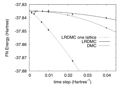
Figure 2: Fixed-node energies for the all-electron carbon atom computed within DMC, single-grid LRDMC (one lattice), and double-grid LRDMC. The lattice discretization parameter $a$ is mapped to the time-step $\tau$ as $a=\sqrt{\tau}$. Reprinted with permission from Casula et al. (2005a), Phys. Rev. Lett., published by APS in 2005.

III Wave functions

Both the accuracy and the computational efficiency of QMC approaches crucially depend on the WF ansatz. The optimal ansatz is typically a tradeoff between accuracy and efficiency. On the one side, a very accurate ansatz can be involved and cumbersome, having many parameters and being expensive to evaluate. On the other hand, an efficient ansatz is described only by the most relevant parameters and can be quickly and easily evaluated. In particular, in sec.II, we have seen that QMC algorithms, both at the variational and fixed-node level, imply several calculations of the local energy $e_{L}(\mathbf{x})$ and the ratio $\Psi(\mathbf{x})/\Psi(\mathbf{x}^{\prime})$ for different electronic configurations $\mathbf{x}$ and $\mathbf{x}^{\prime}$. The computational cost of these operations determines the overall efficiency of QMC and its scaling with systems size.

TurboRVB  employs a many-body WF ansatz $\Psi$ which can be written as the product of two terms:

$$\Psi=\Phi_{\text{AS}}\times\exp J\,,$$ (28)

where the term $\exp J$, conventionally dubbed Jastrow factor, is symmetric under electron exchange, and the term $\Phi_{\text{AS}}$, also referred to as the determinant part of the WF, is antisymmetric. The resulting WF $\Psi$ is antisymmetric, thus fermionic.

In the majority of QMC applications, the chosen $\Phi_{\text{AS}}$ is a single Slater determinant (SD) $\Phi_{\text{SD}}$, i.e., an antisymmetrized product of single-electron WFs. Clearly, SD alone does not include any correlation other than the exchange. However, when a Jastrow factor, explicitly depending on the inter-electronic distances, is applied to $\Phi_{\text{SD}}$ the resulting ansatz $\Psi_{\text{JSD}}=\Phi_{\text{SD}}*\exp J$ often provides over 70% of the correlation energy at the variational level. Thus, the Jastrow factor proves very effective in describing the correlation, employing only a relatively small number of parameters, and therefore providing a very efficient way to improve the ansatz. A Jastrow correlated SD (JSD) function yields a computational cost for QMC simulations – both VMC and FN – about $\propto N^{3}$, namely the same scaling of most DFT codes. Therefore, although QMC has a much larger prefactor, it represents an approach much cheaper than traditional quantum chemistry ones, at least for large enough systems.

While the JSD ansatz is quite satisfactory in several applications, there are situations where very high accuracy is required, and a more advanced ansatz is necessary. The route to improve JSD is not unique, and different approaches have been attempted within the QMC community. First, it should be mentioned that improving the Jastrow factors is not an effective approach to achieve higher accuracy at the FN level, as the Jastrow is positive and cannot change the nodal surface. A popular approach is through the employment of backflow López Ríos et al. (2006), which is a remapping of the electronic configurations that enters into $\Phi_{\text{AS}}$ (SD as a special case) where each electron position is appropriately changed depending on nearby electrons and nuclei. Backflow is an effective way to recover correlation energy, both at the variational and FN level. However, it can be used at a price to increase significantly an already large computational cost. Another possibility is to improve $\Psi_{\text{SD}}$ similarly to conventional quantum chemistry approaches, namely by considering $\Phi_{\text{AS}}$ as a linear expansion of several Slater determinants. While this second approach can provide very high accuracy, it may be extremely expensive, as the number of determinants necessary to remain with a pre-defined accuracy grows combinatorially with the system size.

The vision embraced in TurboRVB, is that the route toward an improved ansatz should not compromise the efficiency and good scaling of QMC. For this reason, neither backflow nor explicit multideterminant expansions are implemented in the code. Within the TurboRVB project, the main goal is instead to consider an ansatz that can be implicitly equivalent to a multideterminant expansion, but remains in practice as efficient as a single determinant. There are five alternatives for the choice of $\Phi_{\text{AS}}$, which correspond to $\rm(\hskip 1.79993pti\hskip 1.79993pt)$ the Pfaffian (Pf), $\rm(\hskip 0.80002ptii\hskip 0.80002pt)$ the Pfaffian with constrained number of molecular orbitals (Pfn) $\rm(iii)$ the Antisymmetrized Geminal Power (AGP), $\rm(iv)$ the Antisymmetrized Geminal Power with constrained number of molecular orbitals (AGPn), and $\rm(\hskip 0.59998ptv\hskip 0.59998pt)$ the single Slater determinant.

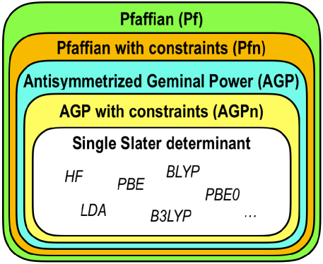
Figure 3: Ansatz hierarchy. The output of Hartree-Fock (HF) or DFT simulations with different exchange-correlation functionals are special instances of the SD ansatz.

It is interesting to observe that all the latter four WFs are obtained by introducing specific constraints on the most general Pf ansatz. The hierarchy of the five ansätze is represented in the Venn diagram of Fig. 3. Clearly, a more general ansatz is more accurate in the total energy but not necessarily in the energy differences. Moreover, it is described by more variational parameters, that could imply a more challenging optimization and a slightly higher cost. TurboRVB  includes several tools to go from one ansatz to another, as represented in Fig. 4. Typically the starting point is SD, which can be obtained from a Hartree-Fock (HF) or a DFT calculation with different exchange-correlation functionals. Both methods are not expected to provide the optimal parameters when the Jastrow factor is included in the WF.

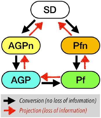
Figure 4: Ansatz conversion.

Indeed, in QMC, the WFs are always meant to include the Jastrow factor, which proves fundamental to improve the properties of the overall WF. For instance, AGP carries more correlation than SD. However, it is not size-consistent unless it is multiplied by a Jastrow factor. Thus, a fundamental step to take advantage of the WF ansatz is the possibility to perform reliable optimizations of the parameters. Optimization will be discussed in section VII. In this section, we will describe the functional form of the Jastrow factor implemented in TurboRVB (sec. III.1), the Pfaffian (sec. III.2), the AGP (sec. III.3), the AGPn and Pfn (sec. III.4), the SD (sec. III.5), the multiconfigurational character of the AGP (sec. III.6), the basis set (sec. III.7), the pseudopotentials (sec. III.8), the contractions of the orbitals (sec. III.9), and the conversion tool (sec. III.10).

III.1 Jastrow factor (J)

The Jastrow factor ($\exp J$) plays an important role in improving the correlation of the WF and in fulfilling Kato’s cusp conditions Kato (1957). TurboRVB  implements the Jastrow term composed of one-body, two-body, and three/four-body factors ($J={J_{1}}+{J_{2}}+{J_{3/4}}$). The one-body and two-body factors are used to fulfill the electron-ion and electron-electron cusp conditions, respectively, and the three/four-body factors are employed to consider a systematic expansion, in principle converging to the most general electron pairs contribution. The one-body Jastrow factor $J_{1}$ is the sum of two parts, the homogeneous part (enforcing the electron-ion cusp condition):

$$J_{1}^{h}\left(\mathbf{r}_{1},\ldots,\mathbf{r}_{N}\right)=\sum_{i=1}^{N}\sum_{a=1}^{N_{\text{at}}}\left({{-{{\left({2{Z_{a}}}\right)}^{3/4}}u_{a}\left({(2{Z_{a}})^{1/4}\left|{{\mathbf{r}_{i}}-{{\mathbf{R}}_{a}}}\right|}\right)}}\right),$$ (29)

and the corresponding inhomogeneous part:

$${J_{1}^{inh}}\left({{{\mathbf{r}}_{1}}{\sigma_{1}},\ldots,{{\mathbf{r}}_{N}}{\sigma_{N}}}\right)=\sum_{i=1}^{N}\sum_{a=1}^{N_{\text{at}}}\left({\sum\limits_{l}{M_{a,l}^{{\sigma_{i}}}\chi_{a,l}\left({{{\mathbf{r}}_{i}}}\right)}}\right),$$ (30)

where ${{{\mathbf{r}}_{i}}}$ are the electron positions, ${{{\mathbf{R}}_{a}}}$ are the atomic positions with corresponding atomic number $Z_{a}$, $l$ runs over atomic orbitals $\chi_{a,l}$ (e.g., GTO) centered on the atom $a$, ${{\sigma_{i}}}$ represents the electron spin ($\uparrow$ or $\downarrow$), $\{M_{a,l}^{\sigma_{i}}\}$ are variational parameters, and ${u_{a}\left(\mathbf{r}\right)}$ is a simple bounded function. In TurboRVB, the most common choice for $u_{a}$ is:

$$u_{a}\left(r\right)=\frac{1}{2b_{\text{e}a}}\left({1-{e^{-rb_{\text{e}a}}}}\right)\,,$$ (31)

depending on a single variational parameter $b_{\text{e}a}$, that may be optimized independently for each atomic species.

The two-body Jastrow factor is defined as:

$${J_{2}}\left({{{\mathbf{r}}_{1}}{\sigma_{1}},\ldots,{{\mathbf{r}}_{N}}{\sigma_{N}}}\right)={\sum\limits_{i<j}{{v_{{\sigma_{i}},{\sigma_{j}}}}\left({\left|{{{\mathbf{r}}_{i}}-{{\mathbf{r}}_{j}}}\right|}\right)}},$$ (32)

where $v_{{\sigma_{i}},{\sigma_{j}}}$ is another simple bounded function. There are several possible choices for $v_{{\sigma_{i}},{\sigma_{j}}}$ implemented in TurboRVB (all listed in the file input.tex in the doc folder), and one of them is, for instance, the following spin-dependent form:

$${v_{{\sigma_{i}},{\sigma_{j}}}}\left({{r_{i,j}}}\right)=\begin{cases}\cfrac{{{r_{i,j}}}}{4}\cdot{\left({1+b_{\rm{ee}}^{\rm{para}}\cdot{{r_{i,j}}}}\right)^{-1}}&({\sigma_{i}}={\sigma_{j}})\\ \cfrac{{{r_{i,j}}}}{2}\cdot{\left({1+b_{\rm{ee}}^{\rm{anti}}\cdot{{r_{i,j}}}}\right)^{-1}}&({\sigma_{i}}\neq{\sigma_{j}})\end{cases}$$ (33)

where ${r_{i,j}}=\left|{{{\mathbf{r}}_{i}}-{{\mathbf{r}}_{j}}}\right|$, and $b_{\rm{ee}}^{\rm{para}}$ and $b_{\rm{ee}}^{\rm{anti}}$ are variational parameters.

The three/four-body Jastrow factor reads:

$$J_{3/4}\left({{{\mathbf{r}}_{1}}{\sigma_{1}},\ldots,{{\mathbf{r}}_{N}}{\sigma_{N}}}\right)=\sum_{i<j}\left(\sum_{a,l}\sum_{b,m}M_{a,l,b,m}^{{\sigma_{i}},{\sigma_{j}}}\chi_{a,l}(\mathbf{r}_{i})\chi_{b,m}(\mathbf{r}_{j})\right),$$ (34)

where the indices $l$ and $m$ again indicate different orbitals centered on corresponding atoms $a$ and $b$, and $\{M_{a,l,b,m}^{\sigma_{i},\sigma_{j}}\}$ are variational parameters. Sometimes it is convenient to set to zero part of the coefficients of the four-body Jastrow factor, namely those corresponding to $a\neq b$, as they increase the overall variational space significantly and make the optimization more challenging, without being much more effective in improving the variational WF.

III.2 Pfaffian Wave function (Pf)

The SD is an antisymmetrized product of single-electron WFs. Thus, SD neglects almost entirely the correlation between electrons. A natural way to improve this description is to include explicitly in the ansatz pairwise correlations among electrons. This is precisely what the Pfaffian WF does.Bajdich et al. (2006, 2008); Genovese et al. (2019a) The building block of the Pfaffian WF is the pairing function $g(\mathbf{i},\mathbf{j})$ between any pair of electrons $i$ and $j$. Henceforth we denote with the generic bolded index $\mathbf{i}$ both the space ${\bf r}_{i}$ coordinates and the spin values $\sigma_{i}$:

$$\mathbf{i}\leftrightarrow({\bf r}_{i},\sigma_{i})$$ (35)

corresponding to the $i^{th}$ electron.

For simplicity, let us first consider a system with an even number $N$ of electrons. The WF, written in terms of pairing functions, is:

$$\Phi_{\text{AS}}(\mathbf{1},\ldots,\mathbf{N})={\cal A}\left\{g(\mathbf{1},\mathbf{2})g(\mathbf{3},\mathbf{4})\ldots g(\mathbf{N-1},\mathbf{N})\right\}$$ (36)

where ${\cal A}$ is the antisymmetrization operator:

$${\cal A}\equiv{1\over N!}\sum_{P\in S_{N}}\epsilon_{P}\hat{P},$$ (37)

$S_{N}$ the permutation group of $N$ elements, $\hat{P}$ the operator corresponding to the generic permutation $P$, and $\epsilon_{P}$ its sign.

Let us define $G$ the $N\times N$ matrix with elements $G_{i,j}=g(\mathbf{i},\mathbf{j})$. Notice that

$$g(\mathbf{i},\mathbf{j})=-g(\mathbf{j},\mathbf{i})\;(\text{and}\;G_{i,j}=-G_{j,i}),$$ (38)

as a consequence of the statistics of fermionic particles, thus $G$ is skew-symmetric (i.e., $G^{T}=-G$, being ^T the transpose operator), so the diagonal is zero and the number of independent entries is $\sum_{n=1}^{N-1}n=N(N-1)/2$.

The PfaffianKasteleyn (1963) of a $N\times N$ skew-symmetrix matrix $G$ is defined as:

$$\text{Pf}(G)\equiv{1\over 2^{N/2}(N/2)!}\sum_{P\in S_{N}}\epsilon_{P}G_{P(1),P(2)}\cdots G_{P(N-1),P(N)}$$ (39)

if $N$ is even, and it is zero if $N$ is odd. Therefore, the WF $\Phi_{\text{AS}}$ defined in the right-hand side (RHS) of Eq. 36 equals ${1\over N!!}\text{Pf}(G)$ where the semifactorial $N!!\equiv{N!\over 2^{N/2}(N/2)!}$ is irrelevant in QMC, as it affects only the normalization of the WF. Thus, we can define our electronic WF as:

$$\Phi_{\text{Pf}}=\text{Pf}(G)\,.$$ (40)

Notice that the $\Phi_{\text{Pf}}$ here defined allows the description of any system with $N_{u}$ electrons with spin-up and $N_{d}$ electrons with spin-down, provided that $N=N_{u}+N_{d}$ is even. Indeed, with no loss of generality, we can assume that electrons $i=1,\ldots,N_{u}$ have $\sigma_{i}=1/2$ and electrons with $i=N_{u}+1,\ldots,N$ have $\sigma_{i}=-1/2$. Thus, the $N\times N$ skew-symmetric matrix $G$ is written as:

$$G=\left[\begin{array}[]{c|c}G_{uu}&G_{ud}\\ \hline\cr G_{du}&G_{dd}\end{array}\right]$$ (41)

where $G_{uu}$ is a $N_{u}\times N_{u}$ skew-symmetric matrix with elements $g_{uu}(\mathbf{i},\mathbf{j})$, $G_{dd}$ is a $N_{d}\times N_{d}$ skew-symmetric matrix with elements $g_{dd}(\mathbf{i},\mathbf{j})$, $G_{ud}$ is a $N_{u}\times N_{d}$ matrix with elements $g_{ud}(\mathbf{i},\mathbf{j})$, and $G_{du}=-{G_{ud}}^{T}$, i.e., $g_{du}(\mathbf{i},\mathbf{j})=-g_{ud}(\mathbf{j},\mathbf{i})$. $g_{uu}$ describes the pairing between a pair of electrons with spin-up:

$$g_{uu}(\mathbf{i},\mathbf{j})=f_{uu}({\bf r}_{i},{\bf r}_{j})\left|\uparrow\uparrow\right\rangle$$ (42)

where the function $f_{uu}$ describes the spatial dependence on the coordinates ${\bf r}_{i},{\bf r}_{j}$ for $i,j\leq N_{u}$. Notice that $f_{uu}({\bf r}_{j},{\bf r}_{i})=-f_{uu}({\bf r}_{i},{\bf r}_{j})$ as a consequence of the properties of $g$. The spin part $\left|\uparrow\uparrow\right\rangle$ describes a system with unit total spin and spin projection along the $z$-axis, and will be indicated by $\left|1,+1\right\rangle$. Similarly, $g_{dd}$ describes the pairing between pairs of electrons with spin-down for $i,j>N_{u}$:

$$g_{dd}(\mathbf{i},\mathbf{j})=f_{dd}({\bf r}_{i},{\bf r}_{j})\left|\downarrow\downarrow\right\rangle$$ (43)

with $f_{dd}({\bf r}_{j},{\bf r}_{i})=-f_{dd}({\bf r}_{i},{\bf r}_{j})$, and the spin part $\left|\downarrow\downarrow\right\rangle$ describes a system with total unit spin and negative spin projection along the $z$-axis, indicated with $\left|1,-1\right\rangle$. $g_{ud}$ describes the pairing between pairs of electrons with unlike spins. Since two electrons with unlike spins can form a singlet $\left|0,0\right\rangle={{\left|\uparrow\downarrow\right\rangle-\left|\downarrow\uparrow\right\rangle}\over\sqrt{2}}$ or a triplet $\left|1,0\right\rangle={{\left|\uparrow\downarrow\right\rangle+\left|\downarrow\uparrow\right\rangle}\over\sqrt{2}}$, in the general case the pairing function $g_{ud}$ will be a linear combination of the the two components:

$$g_{ud}(\mathbf{i},\mathbf{j})=f_{S}({\bf r}_{i},{\bf r}_{j}){{\left|\uparrow\downarrow\right\rangle-\left|\downarrow\uparrow\right\rangle}\over\sqrt{2}}+f_{T}({\bf r}_{i},{\bf r}_{j}){{\left|\uparrow\downarrow\right\rangle+\left|\downarrow\uparrow\right\rangle}\over\sqrt{2}}$$ (44)

where $f_{S}({\bf r}_{i},{\bf r}_{j})=f_{S}({\bf r}_{j},{\bf r}_{i})$ describes the spatial dependence of the singlet part of $g_{ud}$, and $f_{T}({\bf r}_{i},{\bf r}_{j})=-f_{T}({\bf r}_{j},{\bf r}_{i})$ describes the spatial dependence of the triplet part. Therefore, the generic pairing function $g(\mathbf{i},\mathbf{j})$ is the sum of all the four components mentioned above, namely :

$$\begin{split}g\left(\mathbf{i},\mathbf{j}\right)&=f_{S}({\bf r}_{i},{\bf r}_{j})\left|0,0\right\rangle+f_{T}({\bf r}_{i},{\bf r}_{j})\left|1,0\right\rangle\\ &+f_{uu}({\bf r}_{i},{\bf r}_{j})\left|1,+1\right\rangle+f_{dd}({\bf r}_{i},{\bf r}_{j})\left|1,-1\right\rangle\,.\end{split}$$ (45)

The pairing functions $f_{S}$, $f_{T}$, $f_{uu}$, and $f_{dd}$ are expanded over atomic orbitals (see sec. III.7). Say, for a generic pairing function $f$ we have

$$f\left({{{\mathbf{r}}_{i}},{{\mathbf{r}}_{j}}}\right)=\sum\limits_{l,m,a,b}{{{A}_{\left\{{a,l}\right\},\left\{{b,m}\right\}}}{\psi_{a,l}}\left({{{\mathbf{r}}_{i}}}\right){\psi_{b,m}}\left({{{\mathbf{r}}_{j}}}\right)}$$ (46)

where ${\psi_{a,l}}$ and ${\psi_{b,m}}$ are primitive or contracted atomic orbitals, their indices $l$ and $m$ indicate different orbitals centered on atoms $a$ and $b$, while $i$ and $j$ label the electron coordinates. Symmetries on the system, or properties of the underlying pairing function $f$ imply constraints on the coefficients. For instance, the coefficients of $f_{S}$ are such that $A_{\left\{{a,l}\right\},\left\{{b,m}\right\}}=A_{\left\{{b,m}\right\},\left\{{a,l}\right\}}$ because $f_{S}({\bf r}_{i},{\bf r}_{j})=f_{S}({\bf r}_{j},{\bf r}_{i})$, whereas $A_{\left\{{a,l}\right\},\left\{{b,m}\right\}}=-A_{\left\{{b,m}\right\},\left\{{a,l}\right\}}$ for $f_{T}$, $f_{uu}$, and $f_{dd}$.

Let us consider now the remaining case of a system with an odd number of electrons $N$. The simplest way to handle this case is to consider a system with an extra fictitious electron ${\bf N+1}\leftrightarrow(\mathbf{r}_{N+1},\sigma_{N+1})$ that we set at infinity $\mathbf{r}_{N+1}\to\infty$, thus non interacting with all the $N$ physical electrons. The extra matrix elements are easily computed:

$$g(\mathbf{N+1},\mathbf{N+1}) = 0,$$

$$g(\mathbf{i},\mathbf{N+1})=-g(\mathbf{N+1},\mathbf{i}) = \phi({\bf i})~{}~{}~{}{\rm for~{}}i\leq N,$$ (47)

where $\phi({\bf i})\equiv\phi(\mathbf{r}_{i},\sigma_{i})$ can be considered an extra spin dependent unpaired orbital vanishing at infinity.

The antisymmetric part of the WF of the overall system is then:

$$\Phi_{\text{AS}}(\mathbf{1},\ldots,\mathbf{N})={\cal A}\left\{g(\mathbf{1},\mathbf{2})g(\mathbf{3},\mathbf{4})\ldots g(\mathbf{N},\mathbf{N+1})\right\}$$ (48)

where the antisymmetrization operator acts on the (now even) $N+1$ electrons. This is a perfectly allowed $N$ electron fermionic WF, because by definition: $\rm(\hskip 1.79993pti\hskip 1.79993pt)$ it is antisymmetric for all permutations of the $N+1$ particles and in particular for the $N-$ physical ones; $\rm(\hskip 0.80002ptii\hskip 0.80002pt)$ it does not depend by definition on the extra $N+1^{th}$ coordinates and spin as the fictitious particle is at infinity. On the other hand, it is easy to show that this is a nontrivial and nonvanishing WF, because we can use the basic Pfaffian formula in Eq. 39 for the antisymmetrization of the $N+1$ particles and we readily obtain that:

$$\Phi_{\text{Pf}}=\text{Pf}(\tilde{G})\,,$$ (49)

where

$$\tilde{G}=\left[\begin{array}[]{c|c}G&\Phi\\ \hline\cr-\Phi^{T}&0\end{array}\right]$$ (50)

is a $(N+1)\times(N+1)$ skew-symmetric matrix, and $\Phi$ is a $N$-dimensional vector whose elements are $\phi(\textbf{i})$, $i=1,\ldots,N$. Its Pfaffian is quite generally nonvanishing for at least some configuration provided the diagonalization of the Pfaffian (see later) has at least $(N+1)/2$ non-zero eigenvalues (likewise for the Slater determinant it is enough that the $N-$molecular orbitals are linearly independent) and we obtain in this way that the Pfaffian is perfectly defined even in the odd number of electron case.

Finally, we would like to emphasize that the above argument can be generalized to arbitrary number $k$ of unpaired orbitals and arbitrary boundary conditions including calculations on periodic supercells. We can indeed assume at the beginning that, when $N$ is odd (even), we add an odd (even) number $k$ of unpaired orbitals, such that there are $N$ electrons coupled by the matrix $G$ plus $k$ unpaired electrons. The $k$ unpaired electrons are paired with $k$ fictitious electrons (with a pairing function satisfying conditions analogous to those in Eq. III.2). This yields a Pfaffian of even linear dimension $N+k$ of the same form as the one in Eq. 50 but with $\Phi$ being a block $N\times k$ rectangular matrix, determined by $k$ different spin-dependent orbitals. The same argument holds that the antisymmetrized WF is written as the Pfaffian of the corresponding $(N+k)\times(N+k)$ skew-symmetric matrix, and does not depend on the fictitious particle coordinates introduced and therefore is an allowed physical WF antisymmetric over the $N$ physical particles.

A special case that is of interest is when all the $N$ electrons are set to be unpaired (i.e., when $k=N$ and $\Phi$ is a generic $N\times N$ matrix) and it is assumed that there is no pairing among them (i.e., $G=0$ in the $N\times N$ block matrix in Eq. 50). Thus, using a well-known relation of a Pfaffian

$${\text{Pf}\left(\begin{array}[]{c|c}0&\Phi\\ \hline\cr-\Phi^{T}&0\end{array}\right)}=(-1)^{N\times(N-1)\over 2}\det(\Phi),$$ (51)

we recover the standard Slater determinant. In this way, we can clearly see that the Pfaffian represents a quite remarkable generalization of the single determinant picture, and that a larger variational freedom is exploited by allowing pairing correlations with a non zero matrix $G$.

Recently we have noticed that, following the above derivation, it is possible to generalize further the Pfaffian WF ansatz by introducing fictitious particles and relaxing the constraints on the $\tilde{G}$ matrix, even in the lower block diagonal part, that can be assumed to be an arbitrary non-zero skew-symmetric matrix. Work is in progress in order to understand whether this extended formulation can further improve the accuracy within a single Pfaffian WF.

III.3 Antisymmetrized Geminal Power (AGP)

If we consider only the case of a pairing function $g(\mathbf{i},\mathbf{j})$ that is a spin singlet (namely, $f_{uu}$, $f_{dd}$ $f_{T}$ in Eq. 45 are set to zero, yielding $g(\mathbf{i},\mathbf{j})=f_{S}({\bf r}_{i},{\bf r}_{j})\left|0,0\right\rangle$) then we obtain the singlet Antisymmetrized Geminal Power (denoted as AGPs).

Let us consider first an unpolarized system, having an even number $N$ on electrons, and without loss of generality, we can assume that the electrons $i=1,\ldots,N/2$ have spin up and electrons $j=N/2+1,\ldots,N$ have spin down. Then, the matrices $G_{uu}$ and $G_{dd}$ defined in Sec. III.2 are both zero matrices of size $N/2\times N/2$, and the matrix $G_{ud}$ has only the contribution coming from the singlet, that we dub $G_{S}$. The antisymmetrization operator implies the computation of

$${\text{Pf}\left(\begin{array}[]{c|c}0&G_{S}\\ \hline\cr-G_{S}^{T}&0\end{array}\right)}=(-1)^{N/2\times(N/2-1)\over 2}\det(G_{S})$$ (52)

where the equality follows from a property of the Pfaffian (see Eq. 51). The overall sign is arbitrary for a WF; thus the antisymmetrized product of singlet pairs (geminals) is indeed equivalent to the computation of the determinant of the matrix $G_{S}$:

$$\Phi_{\text{AGPs}}=\det(G_{S})\,.$$ (53)

It should be noticed that it is not necessary that the matrix $G_{ud}$ is symmetric to reduce the Pfaffian to a single determinant evaluation. As long as the matrices $G_{uu}$ and $G_{dd}$ are zero, the Pfaffian is indeed equivalent to $\det(G_{ud})$ and describes an antisymmetric WF. However, if $G_{ud}$ is not symmetric the function

$$\Phi_{\text{AGP}}=\det(G_{ud})$$ (54)

is not an eigenstate of the spin. In other terms, there is a spin contamination, similarly to the case of unrestricted HF calculations.

The AGP ansatz can be generalized to describe polarized systems, i.e., systems where the number $N_{u}$ of electrons of spin up is different from the number $N_{d}$ of electrons with spin down. With no loss of generality, we can assume that $N_{u}>N_{d}$, thus the system is constituted by a number $p=N_{d}$ of electron pairs and a number $k=N_{u}-N_{d}$ of unpaired electrons (clearly, $N=N_{u}+N_{d}=2p+k$). We aim at evaluating:

$${\cal A}\left\{g(\mathbf{1},\mathbf{2})\ldots g(\mathbf{2p-1},\mathbf{2p})\phi_{1}(\mathbf{2p+1})\ldots\phi_{k}(\mathbf{N})\right\}.$$ (55)

As above, we assume that the pairing function is zero for like-spin pairs. With no loss of generality, we can assume that electrons $i=1,\ldots,N_{u}$ have spin up and electrons $j=N_{u}+1,\ldots,N$ have spin down. Moreover, as it was done at the end of the previous subsection, we can add $k$ fictitious entries to $g(\mathbf{i},\mathbf{j})$, such that $g(\mathbf{i},\mathbf{N+l})=\phi_{l}(\mathbf{i})$ for $l=1,\ldots,k$ and $i=1,\ldots,N_{u}$. Thus, the antisymmetrization implies the use of Eq. 51, i.e., :

$${\text{Pf}\left(\begin{array}[]{c|c}0&\tilde{G}\\ \hline\cr-\tilde{G}^{T}&0\end{array}\right)}=(-1)^{N_{u}*(N_{u}-1)\over 2}\det(\tilde{G})$$ (56)

with the $N_{u}\times N_{u}$ matrix $\tilde{G}=\left[\begin{array}[]{c|c}G_{ud}&\Phi\end{array}\right]$, the $N_{u}\times N_{d}$ matrix $G_{ud}$ describing the pairing between the $N_{u}$ spin up electrons and the $N_{d}$ spin down electrons, and the $N_{u}\times k$ matrix $\Phi$ describing the $k$ unpaired orbitals. Thus, we need to evaluate:

$$\Phi_{\text{AGP}}=\det(\tilde{G})\,.$$ (57)

One of the most important advantages of the AGP ansatz is that it is equivalent to a linear combination of Slater determinants (i.e., multi configurations), but the computational cost remains at the level of a single-determinant one Casula and Sorella (2003); Zen et al. (2014a, 2015a), see Section III.6. This is especially important for large systems because the naive multireference approach requires an exponentially large number of Slater determinants, which drastically increases the computational cost. The AGP ansatz was applied to the ab initio calculation by M. Casula and S. Sorella  Casula and Sorella (2003) for the first time in 2003; then it has been also implemented in other QMC codes.

III.4 AGP and Pf with constrained number of molecular orbital (AGPn and Pfn)

A convenient way to impose constraints on the variational parameters defining the AGP or Pf WF is obtained by rewriting the expansion of the geminal in terms of molecular orbitals (MOs). As shown in Eq. 46, a geminal $g(\mathbf{i},\mathbf{j})$ is natively expressed in terms of the atomic orbitals $\{\psi_{a,l}({\bf r})\}$, by summing over all the atoms $a$, the corresponding orbitals $l$ and the spin index $\sigma$ (as the elements of the basis may in principle also depend on the spin, even though the most common choice is to take the same orbital for each of the two possible values of the spins). In order to simplify the notation here, let us merge the atomic orbital and spin indices in a unique one that is indicated with a greek symbol (e.g., $\mu\leftrightarrow(a,l)$) running from 1 to the total dimension of the $2L$ atomic orbitals used, $L$ for each spin component. Therefore,

$$g(\mathbf{i},\mathbf{j})=\sum\limits_{\mu,\nu}^{2L}A_{\mu,\nu}\psi_{\mu}(\mathbf{i})\psi_{\nu}(\mathbf{j})$$ (58)

and clearly the symmetry of $g$ implies that $A_{\mu,\nu}=-A_{\nu,\mu}$. The coefficients $A_{\mu,\nu}$ define a $2L\times 2L$ skew-symmetric matrix $A$. If we define the $2L$ dimensional vector $\Psi_{i}=\left(\psi_{1}(\mathbf{i}),\ldots,\psi_{2L}(\mathbf{i})\right)^{T}$, Eq. 58 rewrites as $g(\mathbf{i},\mathbf{j})=\Psi_{i}^{T}A\Psi_{j}$. Moreover, the overlaps $S_{\mu,\nu}\equiv\langle\psi_{\mu}|\psi_{\nu}\rangle$ between atomic orbitals define the overlap matrix $S$, that in the case of a spin-dependent basis is block diagonal:

$$S=\left[\begin{array}[]{c|c}S_{uu}&0\\ \hline\cr 0&S_{dd}\end{array}\right]$$ (59)

with $S_{uu}$ and $S_{dd}$ positive definite $L\times L$ square matrices ($S_{uu}=S_{dd}$ when orbitals are the same for spin up and spin down). In TurboRVB, the overlap matrix $S$ is computed on a suitable uniform mesh with an efficient and general parallel algorithm. Then an orthonormal basis is defined:

$$\tilde{\psi}_{\mu}(\mathbf{i})=\sum\limits_{\nu}S^{-1/2}_{\mu,\nu}\,\psi_{\nu}(\mathbf{i})$$ (60)

where $S^{-1/2}$ is well defined since $S$ is strictly positive definite. The matrix elements of $g$ can be recasted in the new orthonormal basis $\left\{\tilde{\psi}_{\mu}(\mathbf{i})\right\}$, yielding $g(\mathbf{i},\mathbf{j})=\sum_{\mu,\nu}^{2L}\tilde{A}_{\mu,\nu}\tilde{\psi}_{\mu}(\mathbf{i})\tilde{\psi}_{\nu}(\mathbf{j})=\tilde{\Psi}_{i}^{T}\tilde{A}\tilde{\Psi}_{j}$, with the matrix $\tilde{A}\equiv S^{1/2}AS^{1/2}$ that is skew-symmetric.

At this point, from the spectral theory of skew-symmetric matrices, it is possible to perform the Youla decomposition of $\tilde{A}$ (see Ref. Genovese et al., 2020), which can be written in the form $\tilde{A}=Q\Sigma Q^{T}$, where $Q$ is unitary (also real if $\tilde{A}$ is real), and the matrix $\Sigma$ is block diagonal with $\Sigma_{2k-1,2k}=\lambda_{k}=-\Sigma_{2k,2k-1}$ for $k=1,...,L$, and zero everywhere else, with $\lambda_{k}\geq 0$. So, the pairing function $g(\mathbf{i},\mathbf{j})$ can be written as $\Phi_{i}^{T}\Sigma\Phi_{j}$, where $\Phi_{i}=Q^{T}\tilde{\Psi}_{i}$ for each $i$. This defines a basis of $L$ MOs $\left\{\phi_{k}(i)\right\}$ and corresponding twinned ones $\left\{\bar{\phi}_{k}(i)\right\}$, forming together a basis of $2L$ mutually orthonormal elements for which the original geminal function reads:

$$g\left(\mathbf{i},\mathbf{j}\right)=\sum\limits_{k=1}^{L}\lambda_{k}\left[\phi_{k}(\mathbf{i})\bar{\phi}_{k}(\mathbf{j})-\bar{\phi}_{k}(\mathbf{i})\phi_{k}(\mathbf{j})\right]$$ (61)

with $\lambda_{k}\geq 0$. After these transformations these MOs can be finally written in the chosen (hybrid) atomic basis:

$$\phi_{k}(\mathbf{i}) = \sum\limits_{\nu=1}^{2L}P_{\mu,l}\psi_{\mu}(\mathbf{i})$$

$$\bar{\phi}_{k}(\mathbf{i}) = \sum\limits_{\nu=1}^{2L}\bar{P}_{\mu,l}\psi_{\mu}(\mathbf{i})$$ (62)

by appropriate $p\times 2L$ rectangular matrices $P$ and $\bar{P}$. Then, with no loss of generality, we can assume that the molecular orbitals $\left\{\phi_{k}(\mathbf{i}),\bar{\phi}_{k}(\mathbf{i})\right\}$ are ranked such that $\lambda_{1}\geq\lambda_{2}\geq\ldots\geq\lambda_{L}\geq 0$. The above expression highlights that the most important MOs are those corresponding to the larger values of $\lambda_{k}$. Therefore, it is possible to constrain the variational freedom by neglecting all the orbitals with $k>n$, yielding the pairing function:

$$g_{n}\left(\mathbf{i},\mathbf{j}\right)=\sum\limits_{k=1}^{n}\lambda_{k}\left[\phi_{k}(\mathbf{i})\bar{\phi}_{k}(\mathbf{j})-\bar{\phi}_{k}(\mathbf{i})\phi_{k}(\mathbf{j})\right]\,,$$ (63)

where $n$ is conveniently chosen and is $\ll L$. This yields the AGPn ansatz and the $\Phi_{\text{AGPn}}$ WF, which can be useful to improve the stability of the wave-function optimization. The corresponding algorithm (enabled by setting molopt=-1 in the optimization section input of TurboRVB), based on projection operators in the space of the $n$ molecular orbitals considered, has been described extensively in Ref. Becca and Sorella, 2017. Moreover, in the original paperMarchi et al. (2009) introducing the AGPn, a precise recipe was given to improve the evaluation of the binding energies. Indeed, despite a constraint on the variational parameters necessarily increases the variational energy expectation value, energy differences may actually improve by an appropriate choice of $n$. In the mentioned work Marchi et al. (2009), this promising approach was applied with an AGP containing only singlet correlations, but the binding energies were defined without using a rigorous size consistent criterium. This drawback can be now removed, by exploiting the full variational freedom of the Pf WF combined with a general spin-dependent Jastrow factor (see e.g., Fig. 14). Work is in progress in this interesting research direction.

The variational optimization of an AGP with a fixed number $n$ of molecular orbitals can be easily generalized to the Pf case, by exploiting that the constrained Pf WF, dubbed Pfn, can be written either in the canonical form with MOs as in Eq. 63 or in the localized basis set expansion, as in Eq. 58, with a corresponding matrix $A^{n}_{\mu,\nu}=\sum\limits_{k=1}^{n}\lambda_{k}\left[P_{\mu,k}\bar{P}_{\nu,k}-P_{\nu,k}\bar{P}_{\mu,k}\right]$. According to Eq. 63 an arbitrary small variation $\delta g_{n}$ of the constrained pairing function $g_{n}$ reads:

$$\delta g_{n}\left(\mathbf{i},\mathbf{j}\right) = \sum\limits_{k=1}^{n}\delta\lambda_{k}\left[\phi_{k}(\mathbf{i})\bar{\phi}_{k}(\mathbf{j})-\bar{\phi}_{k}(\mathbf{i})\phi_{k}(\mathbf{j})\right]$$ (64)

$$+ \sum\limits_{k=1}^{n}\lambda_{k}\left[\delta\phi_{k}(\mathbf{i})\bar{\phi}_{k}(\mathbf{j})-\delta\bar{\phi}_{k}(\mathbf{i})\phi_{k}(\mathbf{j})\right]$$

$$+ \sum\limits_{k=1}^{n}\lambda_{k}\left[\phi_{k}(\mathbf{i})\delta\bar{\phi}_{k}(\mathbf{j})-\bar{\phi}_{k}(\mathbf{i})\delta\phi_{k}(\mathbf{j})\right]$$

and therefore satisfies the following property, as it will be shown later:

$$(\hat{I}-{\mathbf{L}})\delta g_{n}(\hat{I}-{\mathbf{R}})=0$$ (65)

where $\hat{I}$ is the identity operator, ${\mathbf{L}}$ and ${\mathbf{R}}$ are projection operators over the occupied MOs, i.e., $\mathbf{L}^{2}(\mathbf{i},\mathbf{j})=\int d{\mathbf{k}}\mathbf{L}(\mathbf{i},\mathbf{k})\mathbf{L}(\mathbf{k},\mathbf{j})=\mathbf{L}(\mathbf{i},\mathbf{j})$, and similarly $\mathbf{R}^{2}=\mathbf{R}$, where here and henceforth the shorthand integration symbol $\int d\mathbf{k}=\sum_{\sigma_{k}}\int d\mathbf{r}_{k}$ contains implicitly also the spin summation. These operators are then defined as follows:

$$\mathbf{L}(\mathbf{i},\mathbf{j}) = \sum\limits_{k=1}^{n}\left[\phi_{k}(\mathbf{i})\phi^{*}_{k}(\mathbf{j})+\bar{\phi}_{k}(\mathbf{i})\bar{\phi}^{*}_{k}(\mathbf{j})\right]$$

$$\mathbf{R}(\mathbf{i},\mathbf{j}) = \sum\limits_{k=1}^{n}\left[\phi^{*}_{k}(\mathbf{i})\phi_{k}(\mathbf{j})+\bar{\phi}^{*}_{k}(\mathbf{i})\bar{\phi}_{k}(\mathbf{j})\right].$$ (66)

With the above definitions, Eq. 64 is easily verified because each term of Eq. 64 is annihilated either by the left ($\hat{I}-\mathbf{L}$) or the right ($\hat{I}-\mathbf{R}$) projection over the unoccupied MOs. Notice that $\mathbf{L}=\mathbf{R}$ in the real case and $\mathbf{L}=\mathbf{R}^{*}$ in the most general complex case. In this way, in order to implement a constrained variation $\delta g_{n}$ of the Pfn WF, corresponding to an appropriate variation of its matrix $\delta A^{n}_{\mu,\nu}$, it is useful to work with a small free variation $\delta g$ (with corresponding $\delta A_{\mu,\nu}$). This is then projected onto the chosen restricted ansatz by means of the following equation:

$$\delta g_{n}=\delta g-(\hat{I}-{\bf L})\delta g(\hat{I}-{\bf R}).$$ (67)

Indeed, it is easy to show that the RHS of the above equation vanishes if we apply $\hat{I}-{\bf L}$ and $\hat{I}-{\bf R}$ to its left and its right, respectively, just because $\hat{I}-\mathbf{R}$ and $\hat{I}-\mathbf{L}$ are projection operators, being such $\mathbf{R}$ and $\mathbf{L}$, yielding $(\hat{I}-{\bf R})^{2}=(\hat{I}-{\bf R})$ and $(\hat{I}-{\bf L})^{2}=(\hat{I}-{\bf L})$, from which Eq. 67 fulfills Eq. 65. Eq. 67 represents, therefore, a linear relation applied to the variational parameter matrix change $\delta A_{\mu,\nu}$ corresponding to the unconstrained geminal $g$ in Eq. 58, yielding the new constrained variation $\delta A^{n}_{\mu,\nu}$. Indeed, by using the definitions of the projector operators in Eq. III.4 and the expansion of the MOs in the atomic (hybrid) basis (see Eq. III.4), Eq. 67 turns to a number of matrix-matrix operations acting on $\delta A$, $P$, $\bar{P}$ and the overlap matrix $S$ that can be easily and efficiently implementedBecca and Sorella (2017).

This linear relation between $A$ and $A^{n}$ can be therefore easily implemented together with the corresponding derivatives necessary to the optimization of the energy and allows the explicit calculation of the new matrix $A^{n}_{\mu,\nu}$, yielding the new constrained geminal $g_{n}+\delta g_{n}$. Then the new geminal can be recasted in the form of Eq. 63 by the mentioned diagonalization of skew-symmetric matrices, in this way implicitly neglecting nonlinear contributions that are irrelevant close to convergence, when $\delta g_{n}\to 0$. After employing several iterations of this type, the lowest energy ansatz of the JPfn type can be obtained in a relatively simple and very efficient way.

Finally, it is also important to emphasize that this constrained optimization algorithm allows the reduction of the number of parameters, by efficiently exploiting locality, namely that variational parameters $A_{\mu,\nu}$ corresponding to atoms at a distance larger than a reasonable cutoff (an input named rmax in TurboRVB) can be safely disregarded with negligible errorBecca and Sorella (2017).

III.5 Single Slater determinant (SD)

An important special case of the AGPn and Pfn ansätze discussed in sec. III.4 is when we constrain the pairing function $g_{n}$ to use the minimum possible number of molecular orbitals providing a non zero WF. The minimum number for an unpolarized system with $N$ electrons is equal to the number of electron pairs, that is $n=N/2$. The WF obtained in this way starting from the AGP is indeed the single Slater determinant (SD) Becca and Sorella (2017); Marchi et al. (2009), and we dub it $\Phi_{\text{SD}}$. In principle also the Pfn WF with $n=N/2$ corresponds to a single Slater determinant with spin dependent molecular orbitals, a case that has never been considered so far, but it represents an available option within the most recent versions of TurboRVB.

Similarly, in a polarized system having $N_{u}$ spin up electrons and $N_{d}$ spin down electrons (we assume $N_{u}>N_{d}$), the SD ansatz is obtained by using $N_{u}-N_{d}$ unpaired electrons, and using a constrained pairing function $g_{n}$ with $n=N_{d}/2$.

III.6 Implicit multiconfigurational character of the AGP

In secs. III.2 and  III.3, it has been mentioned that the Pfaffian and the AGP ansätze have a multiconfigurational character, despite they can be evaluated at the cost of a single determinant. In this section, we expand the AGP ansatz in terms of Slater determinants, to show this aspect explicitly. In order to simplify the derivation, we will consider here a simplified case, while the most general case could be studied with a similar approach but involving more cumbersome expressions.

We consider the real AGPs ansatz (Eq. 53) for an unpolarized system of $N=2N_{p}$ electrons (i.e., $N_{u}=N_{d}=N/2$). The symmetry implies that the twin molecular orbitals $\left\{\phi_{k}(\mathbf{i}),\bar{\phi}_{k}(\mathbf{i})\right\}$ appearing in the RHS of Eq. 61 have the same spatial part, that we denote $\tilde{\phi}_{k}(\mathbf{r})$, modulus a sign (because they are orthonormal), and they have opposite spin part. Without loss of generality we can assume that $\phi_{k}$ is spin up and $\bar{\phi}_{k}$ is spin down. Given this convention, the scalar product $l_{k}$ between the spatial parts of $\phi_{k}$ and $\bar{\phi}_{k}$ with either be +1 or -1. We define $\tilde{\lambda}_{k}=l_{k}\lambda_{k}$, where $\lambda_{k}$ is the same as the one in the RHS of Eq. 61. Notice that $\left|\tilde{\lambda}_{k}\right|=\lambda_{k}$, so $\left\{\tilde{\lambda}\right\}$ are ranked in decreasing order of their absolute value (i.e., $\left|\tilde{\lambda}_{k}\right|\geq\left|\tilde{\lambda}_{k+1}\right|$). The pairing function then can be written as

$$g\left(\mathbf{i},\mathbf{j}\right)=\sum_{k=1}^{L}\tilde{\lambda}_{k}\tilde{\phi}_{k}(\mathbf{r}_{i})\tilde{\phi}_{k}(\mathbf{r}_{j})\left({\left|\uparrow\downarrow\right\rangle-\left|\downarrow\uparrow\right\rangle}\right)\,.$$ (68)

This expression is useful for comparing with the standard CI expansion.

It is convenient now to use the second quantization notations in order to simplify the derivation. In particular, we indicate with ${\hat{a}_{k,\uparrow}}^{\dagger}$ (${\hat{a}_{k,\downarrow}}^{\dagger}$) the operator that creates an electron of spin up (down) in the orbitals $\tilde{\phi}_{k}$, and satisfies the canonical anticommutation relations. We can write the pairing functions $g(\mathbf{i},\mathbf{j})\equiv\left<\mathbf{i},\mathbf{j}\middle|\hat{g}\middle|0\right>$, where $\left|0\right>$ is the vacuum, $\left|\mathbf{i},\mathbf{j}\right>$ is the WF of a system with one electron with coordinates $({\bf r}_{i},\sigma_{i})$ and another with coordinates $({\bf r}_{j},\sigma_{j})$, and $\hat{g}$ is the operator:

$$\hat{g}=\sum_{k=1}^{L}\tilde{\lambda}_{k}\hat{a}_{k,\uparrow}^{\dagger}\hat{a}_{k,\downarrow}^{\dagger}\,,$$ (69)

where $\tilde{\lambda}_{k}$ is the one defined above. Using this notation, it is easy to show (see Appendix of Ref. Zen et al., 2015a) that the pairing function $g$ is equivalent to the complete active space of 2 electrons on the $L$ molecular orbitals $\left\{\tilde{\phi}_{k}\right\}$.

Within this notation, the AGPs WF is

$$|\Phi_{\text{AGPs}}\rangle={\hat{g}}^{p}|0\rangle\,,$$ (70)

where $p\equiv N/2$ is the number of electron pairs. If we substitute in ${\hat{g}}^{p}$ the expansion for $\hat{g}$ in Eq. 69, after having conveniently defined the operator $\hat{b}_{k}\equiv\hat{a}_{k,\uparrow}^{\dagger}\hat{a}_{k,\downarrow}^{\dagger}$ which created an electron pair on the orbital $\tilde{\phi}_{k}$, and having noticed that $\hat{b}_{k}\hat{b}_{l}=\hat{b}_{l}\hat{b}_{k}$ and ${\hat{b}_{k}}^{2}=0$ (as following from the anticommutation relations of the $\hat{a}_{k}^{\dagger}$ operators) we obtain that:

$${\hat{g}}^{p}={p!}\sum_{1\leq i_{1}<i_{2}<\ldots<i_{p}\leq L}\tilde{\lambda}_{i_{1}}\tilde{\lambda}_{i_{2}}\ldots\tilde{\lambda}_{i_{p}}\hat{b}_{i_{1}}\hat{b}_{i_{2}}\ldots\hat{b}_{i_{p}}\,.$$ (71)

The chosen order of the $\tilde{\lambda}_{k}$ coefficients implies that the leading term in ${\hat{g}}^{p}$ is given by the term with $(i_{1},\ldots,i_{p})=(1,\ldots,p)$. Thus, we can rewrite ${\hat{g}}^{p}$ in terms of this leading term and excitations with respect to it:

$${{\hat{g}}^{p}\left|0\right>\over p!\prod_{i=1}^{p}\tilde{\lambda}_{i}} = \prod_{i=1}^{p}\hat{b}_{i}|0\rangle+$$

$$+ \sum_{j=1}^{p}\sum_{q=p+1}^{L}{\tilde{\lambda}_{q}\over\tilde{\lambda}_{j}}\left(\mathop{\prod_{i=1}^{p}}_{i\neq j}\hat{b}_{i}\right)\hat{b}_{q}|0\rangle+$$

$$+ \sum_{1\leq j<k\leq{p}}\sum_{{p}<q<r\leq L}{\tilde{\lambda}_{q}\tilde{\lambda}_{r}\over\tilde{\lambda}_{j}\tilde{\lambda}_{k}}\left(\mathop{\prod_{i=1}^{p}}_{i\neq k\land i\neq j}\hat{b}_{i}\right)\hat{b}_{q}\hat{b}_{r}|0\rangle+$$

$$+ \ldots.$$

In the above expansion, we shall recognize that the first element is a single Slater determinant of the molecular orbitals $\left\{\tilde{\phi}_{i}\right\}_{i=1,\ldots,N/2}$; the second element is the summation of all the possible double excitations both going from an orbital $j\leq N/2$ to an orbital $q>N/2$; the third element is the summation of a subset of the possible quadruple excitations, and so on. In other terms, AGPs can be written as the zero seniority subset of the CI expansion, having some constraints on the coefficients of the expansion.

It is worth mentioning that AGPs is also reliable in cases where a single Slater determinant is not a good reference, as for instance, in the case of a broken covalent bond, where the highest occupied molecular orbital (HOMO) and the lowest unoccupied molecular orbital (LUMO) are degenerate (see Fig. 5). In fact, we can have that $\left|\tilde{\lambda}_{p}\right|=\left|\tilde{\lambda}_{p+1}\right|$, so the two determinants $\prod\limits_{i=1}^{p}\hat{b}_{i}\left|0\right>$ and $\left(\prod\limits_{i=1}^{p-1}\hat{b}_{i}\right)\hat{b}_{p+1}\left|0\right>$ have the same weight and they both are the leading terms of the constrained zero-seniority expansion in Eq. III.6.

Notice that in the AGPn ansatz we can perform an expansion similar to Eq. III.6, but the excitations stops at the orbital $n$ rather than $L$. Thus, it is straightforward to see that for $n=N/2$ there are no excitations and the only term is a single Slater determinant.

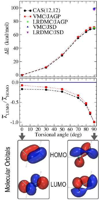
Figure 5: The twisted ethylene molecule (C₂H₄) is a prototypical system requiring a multireference method. The ground state geometry is planar (torsional angle equal to zero); C atoms have a double bond and the HOMO and LUMO orbitals are separated. As the molecule is twisted, one bond is broken and the HOMO-LUMO orbitals become degenerate for a torsional angle of 90 degrees. The upper panel shows evaluations of the torsional barrier as obtained using JSD and JAGP at the VMC and LRDMC level, and using a complete active space (CAS) of 12 orbitals in 12 electrons. JAGP provides reliable results, whereas JSD (which neglects the LUMO orbital) overestimate the barrier both at the variational and diffusion level. The middle panel shows the ratio $\tilde{\lambda}_{\text{LUMO}}/\tilde{\lambda}_{\text{HOMO}}$ in the JAGP ansatz, and the corresponding value in the CAS calculations. The bottom panel shows the HOMO and LUMO orbitals for the planar and twisted geometries. Readapted from Zen et al. (2014a), J. Chem. Theory Comput., published by ACS in 2014.

III.7 Atomic basis set for the pairing function and the Jastrow factor

TurboRVB  employs localized atomic orbitals such as the Gaussian type:

$$\psi_{l,\pm m,I}^{{\text{Gaussian}}}\left({{\mathbf{r}};\zeta}\right)={\left|{{\mathbf{r}}-{{\mathbf{R}}_{I}}}\right|^{l}}{\operatorname{e}^{-\zeta{{\left|{{\mathbf{r}}-{{\mathbf{R}}_{I}}}\right|}^{2}}}}\cdot\Re[(-i)^{1\pm 1\over 2}{Y_{l,m,I}}\left({\theta,\varphi}\right)],$$ (73)

or the Slater type:

$$\psi_{l,\pm m,I}^{{\text{Slater}}}\left({{\mathbf{r}};\zeta}\right)={\left|{{\mathbf{r}}-{{\mathbf{R}}_{I}}}\right|^{l}}{\operatorname{e}^{-\zeta\left|{{\mathbf{r}}-{{\mathbf{R}}_{I}}}\right|}}\cdot\Re[(-i)^{1\pm 1\over 2}{Y_{l,m,I}}\left({\theta,\varphi}\right)],$$ (74)

where the real and the imaginary part ($m>0$) of the spherical harmonic function ${Y_{l,m,I}}\left({\theta,\varphi}\right)$ centered at ${{{\mathbf{R}}_{I}}}$ are (is) taken and rewritten in Cartesian coordinates in order to work with real defined and easy to compute orbitals, $l$ is the corresponding angular momentum and $m\geq 0$ is its projection number along the $z-$quantization axis. The localized atomic orbitals are also present in the onebody and three/four body Jastrow parts (i.e., denoted as $\chi\left({\mathbf{r}}\right)$ in Eq. 30 and Eq. 34). One can use standard basis sets with exponents $\zeta$ (also coefficients for a contracted basis set) taken from the available standard database such as the Basis Set Exchange Pritchard et al. (2019) or from other more specific references when using pseudo potential Trail and Needs (2015); Krogel et al. (2016); Trail and Needs (2017); Bennett et al. (2017, 2018); Annaberdiyev et al. (2018). A python wrapper, named Turbo-Genius, makes the above procedure much easier, as shown later.

III.8 Pseudopotential

TurboRVB  supports pseudopotential calculations both in VMC and LRDMC calculations. Many ECPs have been generated and successfully used in quantum chemistry codes, but they are usually tuned to match Density Functional Theory (DFT) or Hartree-Fock (HF) all-electron (AE) calculations, which are not expected to be optimal for state of the art many-body techniques. Recently some progress has been made in this direction and pseudopotentials determined by correlated many-body techniques are also available Burkatzki et al. (2007, 2008); Trail and Needs (2015); Krogel et al. (2016); Trail and Needs (2017); Bennett et al. (2017, 2018); Annaberdiyev et al. (2018). All the pseudopotentials used in QMC employ the standard semi-local form:

$$\hat{V}_{{\text{pp}}}^{I}\left({{{\mathbf{r}}_{i}}}\right)=V_{{\text{loc}}}^{I}\left({{r_{i,I}}}\right)+\sum\limits_{l=0}^{{l_{\max}}}V_{l}^{I}\left(r_{i,I}\right)\sum\limits_{m=-l}^{l}{\left|{{Y_{l,m}}}\right\rangle\left\langle{{Y_{l,m}}}\right|}$$ (75)

where $r_{i,I}=|{{\mathbf{r}}_{i}}-{{\mathbf{R}}_{I}}|$ is the distance between the $i$-th electron and the $I$-th ions, $l_{{\text{m}ax}}$ is the maximum angular momentum of the ion $I$, and $\sum\limits_{l=0}^{{l_{\max}}}{\sum\limits_{m=-l}^{l}{\left|{{Y_{l,m}}}\right\rangle\left\langle{{Y_{l,m}}}\right|}}$ is a projection operator on the spherical harmonics centered at the ion $I$. In TurboRVB, the angular momentum projector is calculated by using standard polyhedral quadrature formulas for the angular integrationsFahy et al. (1990). As it is now becoming a common practice not only in QMC, both the local $V_{{\text{loc}}}^{I}\left({{r_{i,I}}}\right)$ and the non-local $V_{l}^{I}\left(r_{i,I}\right)$ functions, are expanded over a simple Gaussian basis parametrized by coefficients (e.g., effective charge ${Z_{{\text{eff}}}}$ and other simple constants), multiplying simple powers of $r$, and a corresponding gaussian term:

$${r^{2}}{V_{l}}\left(r\right)=\sum\limits_{k}{{\alpha_{k,l}}{r^{{\beta_{k,l}}}}\exp\left(-{{\gamma_{k,l}}{r^{2}}}\right)},$$ (76)

where ${{\alpha_{k,l}}}$, ${{\beta_{k,l}}}$ (usually small positive integers), and ${{\gamma_{k,l}}}$ are the parameters obtained by appropriate fitting. Several published pseudopotentials have already been tabulated in TurboRVB. Of course, one can also use any pseudopotential employing the semi-local form in the mentioned Gaussian basis with a straightforward little extra work for the input preparation.

III.9 Contraction of the primitive atomic basis

The contraction of atomic orbitals has been widely used in quantum chemistry and DFT codes, and was originally introduced to define a pseudo-Slater orbital by combining several primitive Gaussian orbitals. This is also important in the QMC context because it decreases the number of variational parameters by a large factor, as it will be shown in this section. Although one can obtain a contracted basis set directly from a database, TurboRVB  allows us to prepare a high-quality hybrid basis set (contraction) starting from a given primitive basis, by the so-called “geminal embedding scheme”. Sorella et al. (2015) To this purpose, let us decompose the genimal function in terms of atomic contribution, as far as the dependence over ${\mathbf{i}}$ (the left argument) is concerned:

$$g\left({\mathbf{i},\mathbf{j}}\right)=\sum\limits_{I}{U_{{\text{proj}}}^{I}\left({\mathbf{i},\mathbf{j}}\right)}=\sum\limits_{I}{\sum\limits_{\mu,\nu}{A_{\mu,\nu}^{I}}}{\phi_{\mu}}\left(\mathbf{i}\right){\phi_{\nu}}\left(\mathbf{j}\right),$$ (77)

where $I$ represents an atom in a system, $U_{{\text{proj}}}^{I}\left({\mathbf{i},\mathbf{j}}\right)$ is the pairing function projected on the atom $I$, $A_{\mu,\nu}^{I}$ is ${A_{\mu,\nu}}$ if $\mu\in I$, otherwise ${A_{\mu,\nu}^{I}}=0$, where $A_{\mu,\nu}$ is assumed to be given for the system under consideration, e.g., obtained by a standard DFT calculation, where in this case, by Eq. 63:

$$A_{\mu,\nu}=\sum\limits_{k=1}^{n}\left(c^{k}_{\mu}\bar{c}^{k}_{\nu}-\bar{c}^{k}_{\mu}c^{k}_{\nu}\right)$$ (78)

where $c^{k}_{\mu}$ and $\bar{c}^{k}_{\mu}$ are the coefficients of the DFT molecular orbitals $\phi_{k}({\mathbf{i}})=\sum_{\mu}c^{k}_{\mu}\phi_{\mu}({\mathbf{i}})$ and $\bar{\phi}_{k}({\mathbf{i}})=\sum_{\nu}\bar{c}^{k}_{\nu}\phi_{\nu}({\mathbf{i}})$ in the atomic basis expansion, respectively.

Quite generally, the projected pairing function can be expanded in a truncated space spanned by $q$ terms:

$$\tilde{U}_{{\text{proj}}}^{I}\left({\mathbf{i},\mathbf{j}}\right)=\sum\limits_{k=1}^{q}{{\sigma_{k}}\psi_{k}^{{\text{GEO}}}\left(\mathbf{i}\right)\psi_{k}^{{\text{Env}}}\left(\mathbf{j}\right)}.$$ (79)

In other words, the Schmidt decomposition is applied to the matrix $\tilde{U}_{{\text{proj}}}^{I}\left({\mathbf{i},\mathbf{j}}\right)$ describing the coupling between a given atom $I$ and the enviroment, within the geminal ansatz. This procedure defines the so-called geminal embedded orbitals (GEOs), that are determined in terms of an expansion over all the atomic orbitals used for the atom $I$:

$$\psi_{k}^{{\text{GEO}}}\left(\mathbf{i}\right)=\sum\limits_{\mu\in I}{\mu_{k,\mu}^{{\text{GEO}}}\psi_{\mu}\left(\mathbf{i}\right)},$$ (80)

where $\psi_{k}^{{\text{GEO}}}\left(\mathbf{i}\right)$ are orthonormal. Following the Schmidt decomposition, it is possible to determine the best GEOs by minimizing the Euclidian distance between the original and the truncated geminal functions:

$${d^{2}}={\left|{U_{{\text{proj}}}^{I}-\tilde{U}_{{\text{proj}}}^{I}}\right|^{2}}.$$ (81)

Considering all possible unconstrained functions $\psi_{k}^{{\text{Env}}}\left(\mathbf{j}\right)$ and employing the steady condition $\frac{{\delta{d^{2}}}}{{\delta\psi_{k}^{{\text{Env}}}\left(\mathbf{j}\right)}}=0$, ${{d^{2}}}$ reads:

$${d^{2}}={\left|{U_{{\text{proj}}}^{I}}\right|^{2}}-\sum\limits_{k=1}^{p}{\int{d\mathbf{i}d\mathbf{j}D_{{\text{proj}}}^{I}\left({\mathbf{i},\mathbf{j}}\right)\psi_{k}^{{\text{GEO}}}\left(\mathbf{i}\right)\psi_{k}^{{\text{GEO}}}\left(\mathbf{j}\right)}},$$ (82)

where ${\left|{U_{{\text{proj}}}^{I}}\right|^{2}}=\int{d\mathbf{i}d\mathbf{j}{{\left|{U_{{\text{proj}}}^{I}\left({\mathbf{i},\mathbf{j}}\right)}\right|}^{2}}}$ and $D_{{\text{proj}}}^{I}\left({\mathbf{i},\mathbf{j}}\right)$ is the density matrix that reads:

$$D_{{\text{proj}}}^{I}\left({\mathbf{i},\mathbf{j}}\right)=\int{d\mathbf{k}U_{{\text{proj}}}^{I}\left({\mathbf{i},\mathbf{k}}\right)^{*}U_{{\text{proj}}}^{I}\left({\mathbf{j},\mathbf{k}}\right)}.$$ (83)

Since the GEOs ${\psi_{k}^{{\text{GEO}}}\left({\mathbf{r}}\right)}$ are orthonormal and the density matrix is hermitian, Eq. 82 becomes minimum when the GEOs coincides with the $p$ eigenvectors of the density matrix with the maximum eigenvalues (denoted as ${w_{i}}$). The original atomic basis $\psi_{\mu}\left(\mathbf{i}\right)$ is usually non-orthogonal, so the problem turns into the generalized eigenvalue equation:

$$\sum\limits_{j\in J}{{{\left[{\left({{\bm{A}^{I}{}^{*}}{\bm{S}}{\bm{A}^{I}}}\right){\bm{S}}}\right]}_{i,j}}\mu_{k,j}^{{\text{GEO}}}}={\omega_{k}}\mu_{k,i}^{{\text{GEO}}}.$$ (84)

The truncation error is readily estimated by the summation of the eigenvalues ${d^{2}}={\left|{U_{{\text{proj}}}^{I}}\right|^{2}}-\sum\nolimits_{i=1}^{p}{{w_{p}}}$. Since the eigenvalues are sorted in ascending order, a suitably chosen value of $p$ allows the user to neglect the most irrelevant vector components with small eigenvalues $w_{i}$ and work with enough accuracy even with a few GEOs per atom, thus minimizing the number of variational parameters necessary to describe well the system, as it will be shown below. With this construction a new geminal is defined in the GEO basis, namely:

$$\tilde{g}\left({\mathbf{i},\mathbf{j}}\right)=\sum\limits_{\mu,\nu}{{{\tilde{A}}_{\mu,\nu}}\psi_{\mu}^{{\text{GEO}}}\left(\mathbf{i}\right)\psi_{\nu}^{{\text{GEO}}}\left(\mathbf{j}\right)}$$ (85)

where the matrix coefficients ${{\tilde{A}}_{\mu,\nu}}$ are given by maximizing the normalized overlap ($Q$) between the original and the new geminals:

$$Q=\frac{\braket{{\tilde{g}}}{{g}}^{2}}{\braket{{\tilde{g}}}{{\tilde{g}}}\braket{{g}}{{g}}},$$ (86)

where $\braket{{\tilde{g}}}{{g}}=\int{d\mathbf{i}d\mathbf{j}\tilde{g}\left({\mathbf{i},\mathbf{j}}\right)^{*}g\left({\mathbf{i},\mathbf{j}}\right)}$. It turns out that the overlap remains large even for small GEO basis set size $p$; implying that, by using this scheme, one can decrease the number of variational parameters corresponding to the matrix $A$, i.e., from $4L^{2}$ to $4p^{2}\ll 4L^{2}.$

III.10 Conversion of the WF

As described in Sec. III, TurboRVB implements different types of ansatz: $\rm(\hskip 1.79993pti\hskip 1.79993pt)$ the Pfaffian (Pf), $\rm(\hskip 0.80002ptii\hskip 0.80002pt)$ the Pfaffian with constrained number of molecular orbitals (Pfn) $\rm(iii)$ the Antisymmetrized Geminal Power (AGP), $\rm(iv)$ the Antisymmetrized Geminal Power with constrained number of molecular orbitals (AGPn), and $\rm(\hskip 0.59998ptv\hskip 0.59998pt)$ the single Slater determinant (SD). One can choose a proper ansatz depending on a target system, considering the computational cost of a chosen ansatz and the relevant physical and chemical properties of a target material. During the simulation, a user can go back and forth between the ansatz using modules implemented in TurboRVB, with/without losing the information of an optimized ansatz (see Fig. 4): The first case is to add molecular orbitals to an ansatz, i.e., JAGP $\Rightarrow$ JSD, JAGP $\Rightarrow$ JAGPn, or JPf $\Rightarrow$ JPfn. In TurboRVB, this is obtained by rewriting the expansion of the geminal in terms of molecular orbitals (see sec. III.4 and sec. III.5). The corresponding tool is convertfort10mol.x. The second important case is to convert an ansatz among the available ones, i.e., JSD, JAGP, or JAGPn $\Rightarrow$ JAGP. In TurboRVB, this is the purpose of the convertfort10.x tool and is achieved by maximizing the overlap between the two WFs, one of them being the input (fort.10_in) and the other being the type (fort.10_out) to be filled by new geminal matrix coefficients (result written in fort.10_new). In more details, in TurboRVB, the following overlap between two geminals is maximized:

$$\max Q=\frac{\braket{{g}^{{\text{new}}}}{{g}^{{\text{ori}}}}^{2}}{\braket{{g}^{{\text{new}}}}{{g}^{{\text{new}}}}\braket{{g}^{{\text{ori}}}}{{g}^{{\text{ori}}}}},$$ (87)

in order to obtain new geminal matrix coefficients ${A_{\mu,\nu}^{{\text{new}}}}$, defining the new pairing function as:

$${g^{{\text{new}}}}\left({\mathbf{i},\mathbf{j}}\right)=\sum\limits_{\mu.\nu}{A_{\mu.\nu}^{{\text{new}}}\psi_{\mu}^{{\text{new}}}\left(\mathbf{i}\right)\psi_{\nu}^{{\text{new}}}\left(\mathbf{j}\right)},$$ (88)

while the original geminal was given in terms of the parameter matrix $A_{\mu,\nu}^{\text{ori}}$:

$${g^{{\text{ori}}}}\left({\mathbf{i},\mathbf{j}}\right)=\sum\limits_{\mu,\nu}{A_{\mu,\nu}^{{\text{ori}}}\psi_{\mu}^{{\text{ori}}}\left(\mathbf{i}\right)\psi_{\nu}^{{\text{ori}}}\left(\mathbf{j}\right)}.$$ (89)

Notice that $0\leqslant Q\leqslant 1$; therefore the larger is $Q$, the better is the conversion, and $Q$ approaches the unit value if the conversion is perfect. For this type of conversion, one can also apply the geminal embedding scheme to construct a hybrid basis set, as described in the sec.III.9.

The final case is to convert a JAGP ansatz to JPf. Since the JAGP ansatz is a special case of the JPf one, where only $G_{ud}$ and $G_{du}$ terms are defined as described in the section III.3, the conversion can be realized just by direct substitution. Therefore, the main challenge is to find a reasonable initialization for the two spin-triplet sectors $G_{uu}$ and $G_{dd}$ that are not described in the JAGP and that otherwise have to be set to $0$. There are two possible approaches Genovese et al. (2019a, 2020): $\rm(\hskip 1.79993pti\hskip 1.79993pt)$ for polarized systems, we can build the $G_{uu}$ block of the matrix by using an even number of unpaired orbitals $\{\phi_{i}\}$ and build an antisymmetric $g_{uu}$ by means of Eq. 63, where the eigenvalues $\lambda_{k}$ are chosen to be large enough to occupy certainly these unpaired states, as in the standard Slater determinant used for our initialization. Again, we emphasize that this works only for polarized systems. $\rm(\hskip 0.80002ptii\hskip 0.80002pt)$ The second approach that also works in a spin-unpolarized case is to determine a standard broken symmetry single determinant ansatz (e.g., by the TurboRVB built-in DFT within the LSDA) and modify it with a global spin rotation. Indeed, in the presence of finite local magnetic moments, it is often convenient to rotate the spin moments of the WF in a direction perpendicular to the spin quantization axis chosen for our spin-dependent Jastrow factor, i.e., the $z$ quantization axis. In this way one can obtain reasonable initializations for $G_{uu}$ and $G_{dd}$. TurboRVB allows every possible rotation, including an arbitrary small one close to the identity. A particularly important case is when a rotation of $\pi/2$ is applied around the $y$ direction. This operation maps

$$|\uparrow\rangle\rightarrow\frac{1}{\sqrt{2}}\left(|\uparrow\rangle+|\downarrow\rangle\right)\mbox{ and }|\downarrow\rangle\rightarrow\frac{1}{\sqrt{2}}\left(|\uparrow\rangle-|\downarrow\rangle\right).$$ (90)

One can convert from a AGP the pairing function that is obtained from a VMC optimization:

$${g_{ud}}(\mathbf{i},\mathbf{j})={f_{S}}({{\mathbf{r}}_{i}},{{\mathbf{r}}_{j}})\frac{{\left|{\uparrow\downarrow}\right\rangle-\left|{\downarrow\uparrow}\right\rangle}}{{\sqrt{2}}}+{f_{T}}({{\mathbf{r}}_{i}},{{\mathbf{r}}_{j}})\frac{{\left|{\uparrow\downarrow}\right\rangle+\left|{\downarrow\uparrow}\right\rangle}}{{\sqrt{2}}}$$ (91)

to a Pf one:

$${g_{ud}}(\mathbf{i},\mathbf{j})\to g\left({\mathbf{i},\mathbf{j}}\right){\text{ }}={f_{S}}({{\mathbf{r}}_{i}},{{\mathbf{r}}_{j}})\frac{{\left|{\uparrow\downarrow}\right\rangle-\left|{\downarrow\uparrow}\right\rangle}}{{\sqrt{2}}}+{f_{T}}({{\mathbf{r}}_{i}},{{\mathbf{r}}_{j}})\left({\left|{\uparrow\uparrow}\right\rangle-\left|{\downarrow\downarrow}\right\rangle}\right).$$ (92)

This transformation provides a meaningful initialization to the Pfaffian WF that can be then optimized for reaching the best possible description of the ground state within this ansatz.

IV Bulk systems

The application of TurboRVB  is not limited to open systems such as atoms and molecules. TurboRVB  can also simulate bulk systems in large supercells with arbitrary twisted boundary conditions. These are used to minimize finite-size effects, and represent quite an important approachLin et al. (2001); Dagrada et al. (2016) in order to reach a meaningful and accurate thermodynamic limit.

IV.1 CRYSTAL basis set

For periodic system calculations, the many-body WF should satisfy the many-body Bloch condition Rajagopal et al. (1994, 1995):

$${\Psi_{{k_{s}}}}\left({{{\mathbf{r}}_{1}},\ldots,{{\mathbf{r}}_{i}}+{{\mathbf{T}}_{s}}\ldots,{{\mathbf{r}}_{N}}}\right)={e^{i{{\mathbf{k}}_{s}}\cdot{{\mathbf{T}}_{s}}}}{\Psi_{{k_{s}}}}\left({{{\mathbf{r}}_{1}},\ldots,{{\mathbf{r}}_{i}},\ldots,{{\mathbf{r}}_{N}}}\right),$$ (93)

which follows from the property that the many-body Hamiltonian is invariant under the translation of any electron coordinate by a simulation-cell vector ${\mathbf{T}_{s}}$, where ${{\mathbf{T}}_{s}}=l{\mathbf{a}}+m{\mathbf{b}}+n{\mathbf{c}}$ is determined by arbitrary integers $l,n,m$ and the three vectors ${\mathbf{a}},{\mathbf{b}}$ and ${\mathbf{c}}$ define the supercell.

In TurboRVB, a single-particle basis set satisfies the following condition:

$$\psi_{l,m,I}^{{\text{PBC}}}\left({{\mathbf{r}}+{{\mathbf{T}}_{s}};\zeta}\right)={e^{i{{\mathbf{k}}_{s}}\cdot{{\mathbf{T}}_{s}}}}\psi_{l,m,I}^{{\text{PBC}}}\left({{\mathbf{r}};\zeta}\right)$$ (94)

where ${{{\mathbf{k}}_{{s}}}}$ is a twist vector (${{\mathbf{k}}_{{s}}}=\left({k_{s}^{x},k_{s}^{y},k_{s}^{z}}\right)$), and ${{\mathbf{T}}_{s}}$ represents an arbitrary simulation cell vector. Notice that the use of a non vanishing twist vector generally makes a many-body WF complex. TurboRVB  implements the CRYSTAL periodic basis Pisani et al. (1988); Becca and Sorella (2017); Dovesi et al. (2018):

$$\psi_{l,m,I}^{{\text{PBC}}}\left({{\mathbf{r}};\zeta}\right)=\sum\limits_{{{\mathbf{T}}_{s}}}{\psi_{l,m,I}\left({{\mathbf{r}}+{{\mathbf{T}}_{s}};\zeta}\right){e^{-i{{\mathbf{k}}_{s}}\cdot{{\mathbf{T}}_{s}}}}}$$ (95)

where ${\psi_{l,m,I}}$ is a non-periodic real atomic orbital such as Gaussian (Eq. 73) and Slater (Eq. 74). The use of Gaussian or Slater orbitals that rapidly decay far from nuclei guarantees that the above summation converges fast with a finite small number of ${\mathbf{T}_{s}}$. Notice that, in TurboRVB, ${\mathbf{T}_{s}}$ are not limited to orthorhombic ones but has been recently extended to include all possible crystal translation groups (e.g., rhombohedral, hexagonal, triclinic).

The same procedure is applied to the basis set for the Jastrow part, although using simple periodic boundary conditions Becca and Sorella (2017), because the twists do not affect the Jastrow part of the WF, namely:

$$\chi_{l,m,I}^{{\text{PBC}}}\left({{\mathbf{r}};\zeta}\right)=\sum\limits_{\mathbf{T}_{s}}{\chi_{l,m,I}\left({{\mathbf{r}}+{{\mathbf{T}}_{s}};\zeta}\right)},$$ (96)

which satisfies $\chi_{l,m,I}^{{\text{PBC}}}\left({{\mathbf{r}}+{{\mathbf{T}}_{s}};\zeta}\right)=\chi_{l,m,I}^{{\text{PBC}}}\left({{\mathbf{r}};\zeta}\right)$.

Moreover, the homogeneous one-body and two-body Jastrow factors have to be appropriately periodized because they are not defined in terms of the above periodic basis. Namely, the homogeneous one-body Jastrow part (Eq. 30) should satisfy:

$${{\tilde{J}}_{1}}\left({{\mathbf{r}}+{{\mathbf{T}}_{s}}}\right)={{\tilde{J}}_{1}}\left({\mathbf{r}}\right),$$ (97)

and the two-body Jastrow part (Eq. 32) should fulfill:

$${J_{2}}\left({{{\mathbf{r}}_{1}}{\sigma_{1}},\ldots,\left({{{\mathbf{r}}_{i}}+{{\mathbf{T}}_{s}}}\right){\sigma_{i}},\ldots{{\mathbf{r}}_{N}}{\sigma_{N}}}\right)={J_{2}}\left({{{\mathbf{r}}_{1}}{\sigma_{1}},\ldots,{{\mathbf{r}}_{i}}{\sigma_{i}},\ldots{{\mathbf{r}}_{N}}{\sigma_{N}}}\right).$$ (98)

In order to satisfy the above constraints, we consider the relative electron-nuclei or electron-electron coordinate differences ${\mathbf{r}}_{d}$, necessary to evaluate $J_{1}$ and $J_{2}$, respectively, and expand them as:

$${\mathbf{r}}_{d}=r_{a}{\mathbf{a}}+r_{b}{\mathbf{b}}+r_{c}{\mathbf{c}},$$ (99)

where $r_{a},r_{b}$ and $r_{c}$ are appropriate transformed coordinates, that are conveniently defined within a cube of unit length, because of the assumed periodicity of the supercell, namely $|r_{a}|,|r_{b}|,|r_{c}|<1/2$. As a consequence, this mapping makes the physical electron-electron and electron-ion distance periodic by definition (i.e., they refer to the minimum distance image of the supercell). However, there may be divergences or singularity at the boundaries of this unit cube. Therefore, before computing the distance corresponding to ${\mathbf{r}}_{d}$, these coordinates are transformed $\left(r_{a},r_{b},r_{c}\right)\to\left(\bar{r}_{a},\bar{r}_{b},\bar{r}_{c}\right)=\left(p(r_{a}),p(r_{b}),p(r_{c})\right)$ by use of an appropriate function $p(x)$, with at least continuous first derivative for $|x|<1/2$. This function is chosen to preserve the physical meaning at short distances, i.e., $p(x)=x$ in these cases, and being nonlinear elsewhere, in order to satisfy not only the periodicity but also the requirement of continuous first derivatives of the many-body WF $\Psi_{k_{s}}$. We have, therefore, defined $p(x)$ as follows:

$$p\left(x\right)=\begin{cases}x&(-\frac{1}{4}<x<\frac{1}{4})\\ -{1\over 8(1+2x)}&(-\frac{1}{2}\leqslant x\leqslant-\frac{1}{4})\\ {1\over 8(1-2x)}&(\frac{1}{4}\leqslant x\leqslant\frac{1}{2}).\end{cases}$$ (100)

Indeed, though the modified relative distance diverges (i.e., $\left|{{\mathbf{r}}_{d}}\right|\to\infty$) at the edges of the Wigner-Seitz cell (e.g., ${\mathbf{r}}=\pm\frac{1}{2}{\mathbf{a}},\pm\frac{1}{2}{\mathbf{b}},\pm\frac{1}{2}{\mathbf{c}}$), the exponential (Eq. 31) and the Padé (Eq. 33) functions remain finite, $u\left(r\right)\to 1/2b_{\text{e}a}$ and ${v_{{\sigma_{i}},{\sigma_{j}}}}\left({{r_{i,j}}}\right)\to 1/4b_{\rm{ee}}^{\rm{para}}$ or $1/2b_{\rm{ee}}^{\rm{anti}}$, respectively, thus preserving with continuity the periodicity of the one-/two- body homogeneous parts of the Jastrow factor. However, for the Padé form, one has to change the expression for $p(x)$ in order to satisfy also the continuity in the WF derivatives, even when the modified relative distances diverge, i.e.,:

$$p\left(x\right)=\begin{cases}x&(-\frac{1}{6}<x<\frac{1}{6})\\ -{1\over 54(1/2+x)^{2}}&(-\frac{1}{2}\leqslant x\leqslant-\frac{1}{6})\\ {1\over 54(1/2-x)^{2}}&(\frac{1}{6}\leqslant x\leqslant\frac{1}{2}).\end{cases}$$ (101)

In this case the region where $p(x)=x$ further shrinks. Thus, it is often more convenient to use the exponential form to obtain a more accurate variational WF, because the long-range part is implicitly corrected by the inhomogeneous terms in Eq. 34.

Finally, we remark that the many-body WF also obeys the second Bloch condition Rajagopal et al. (1994, 1995), namely:

$${\Psi_{{k_{p}}}}\left({\left\{{{{\mathbf{r}}_{i}}+{{\mathbf{T}}_{p}}}\right\}}\right)={e^{i{{\mathbf{k}}_{p}}\cdot{{\mathbf{T}}_{p}}}}{\Psi_{{k_{p}}}}\left({\left\{{{{\mathbf{r}}_{i}}}\right\}}\right),$$ (102)

where ${\mathbf{T}_{p}}$ represents a unit-cell (not supercell) vector, and ${{{\mathbf{k}}_{p}}}$ is the crystal momentum. This comes from the property that the many-body Hamiltonian is invariant under the simultaneous translation of all-electron coordinates by a unit-cell vector ${\mathbf{T}_{p}}$. Within TurboRVB, this condition can be employed by imposing the intra-unit cell translational symmetries on the Jastrow and the pairing function, as simple linear constraints in the variational parameters. However, this option is restricted to the case ${{{\mathbf{k}}_{p}}}=0$. On the other hand, it is possible to use different twists on each spin component, that has proven very effective for implementing the mentioned translation symmetries within pairing WFs.Karakuzu et al. (2017)

IV.2 Finite-size effects

The systematic error induced by a finite simulation cell is a long-standing issue in the ab initio QMC calculation. There are two types of finite-size errors in QMC calculations; one is the so-called one-body effect that arises from the kinetic energy term of the Hamiltonian, and the other one is the so-called two-body effect that arises from the periodic Ewald contribution resulting from the electron-electron interaction. Notice that, in the independent-particle calculations (i.e., DFT), only the former is present, which can be readily evaluated by $k$ summation in the first Brillouin zone, but the two-body finite-size effects are not present because the exchange-correlation energy used in DFT usually derives from DMC results extrapolated to the infinite simulation cell size. To correct the one-body finite-size error, one can use the twisted averaged boundary conditions Lin et al. (2001), special $k$-points methods Rajagopal et al. (1994, 1995), or the exact special twist (EST) method Dagrada et al. (2016), all of which have been implemented in TurboRVB. Within the TurboRVB implementation, the Jastrow part is independent of twists (i.e., TurboRVB uses a common Jastrow for all twists),

$${\Psi_{{k_{s}}}}\left({{{\mathbf{r}}_{1}},\ldots,{{\mathbf{r}}_{N}}}\right)=J\left({{{\mathbf{r}}_{1}},\ldots,{{\mathbf{r}}_{N}}}\right)\Phi_{AS}^{{}_{{k_{s}}}}\left({{{\mathbf{r}}_{1}},\ldots,{{\mathbf{r}}_{N}}}\right).$$ (103)

As emphasized in Ref. Lin et al., 2001, at variance with DFT, the QMC computational effort is independent of the number of $k$-points used. For the two-body finite-size effects, which cannot be alleviated by the above remedy, one can employ the model periodic Coulomb interaction (MPC) Fraser et al. (1996); Williamson et al. (1997); Kent et al. (1999). This method has not been implemented in TurboRVB yet. Nevertheless, simpler alternatives exist. For instance one can alleviate the two-body finite size effects by directly increasing the supercell size, or one can estimate these effects by employing the KZK exchange-correlation function Kwee et al. (2008) at the DFT level. Moreover, it is also possible to employ systematic finite-size corrections based on the knowledge of the density structure factor in momentum spaceChiesa et al. (2006), that can be readily computed within TurboRVB, with a short postprocessing computation.

V Built-in Density Functional theory (DFT) code

Although most QMC codes load their trial WFs from available DFT/quantum chemistry codes such as Gaussian Frisch et al. (2016), CRYSTAL Dovesi et al. (2018), and Quantum Espresso Giannozzi et al. (2009), TurboRVB is a self-consistent many-body package and does not require input from other codes. Indeed, in TurboRVB, an original DFT code is implemented that has the important feature to work in exactly the same basis and pseudopotentials (if any) used for the QMC many-body WF, and for instance can work with mixed Slater-Gaussian basis or with arbitrary contraction, i.e., mixing angular momenta. On the other hand, the drawback is that only very few functionals are available so far because, within the TurboRVB approach, the DFT has to be used only to have a reasonable initialization of the antisymmetric part of the many-body WF. This is then optimized at best by direct minimization of the energy in the presence of the Jastrow factor and should very weakly depend on the initialization, or for instance, on the DFT functional used. At present, TurboRVB  supports Perdew-Zunger (PZ81) Local-Spin Density Approximation (LSDA)Perdew and Zunger (1981), and those combined with KZK exchange-correlation energy Kwee et al. (2008), but, for instance, does not allow LDA + $U$ calculations. This will be the goal of a possible future work.

V.1 Stabilization algorithm for large localized basis sets

An important issue in any DFT algorithm based on localized basis sets, such as Gaussian, is how to reach the so-called complete basis set limit. In the plane-wave method, this is systematically achieved by increasing the number of plane waves (e.g., kinetic cutoff energy). However, with a localized basis set, by increasing its dimension, numerical instabilities may occur as a consequence of the redundancy and non-orthonormality of the basis. On the other hand, the use of a small basis set implies too much biased results. In TurboRVB, an original and systematic algorithm to remove this redundancyAzadi et al. (2010) has been implemented. When the basis set is non-orthogonal, the key self consistent step for solving the DFT Kohn-Sham equations, turns to a generalized eigenvalue problem:

$${\bm{\mathcal{H}}}{\mathbf{c}}=E{\mathbf{S}}{\mathbf{c}},$$ (104)

where ${\bm{\mathcal{H}}}$ is the single-particle Hamiltonian matrix, ${\mathbf{c}}$ is the vector of the coefficients of the orbitals, $E$ is the single-particle energy, and the ${\mathbf{S}}$ is the $N_{b}$ $\times$ $N_{b}$ overlap matrix, where $N_{b}$ is the dimension of the basis set:

$${S_{i,j}}=\braket{{{{\phi_{i}}}}}{{{{\phi_{j}}}}}=\int{d{\mathbf{r}}{\phi_{i}^{*}}\left({\mathbf{r}}\right){\phi_{j}}\left({\mathbf{r}}\right)}.$$ (105)

The overlap matrix is strictly positive definite, namely all its eigenvalues are positive. The problem mentioned above shows up when the overlap matrix ${\mathbf{S}}$ becomes ill-conditioned. If the condition number, namely the ratio between the largest (denoted as $s_{N_{b}}$) and the smallest eigenvalues (denoted as $s_{1}$), becomes very large, the CBS limit cannot be achieved by the standard procedure due to numerical instabilities. Therefore, in TurboRVB, the small eigenvalues and the corresponding eigenvectors are disregarded. Indeed, the original basis is modified as follows:

$$e_{j}^{i}=\frac{1}{{\sqrt{{s_{i}}}}}\upsilon_{j}^{i}\,\,{\text{for}}\,\,{s_{i}}/{s_{N}}\geqslant{\varepsilon_{{\text{mach}}}},$$ (106)

where ${{{s}_{i}}}$ and $\upsilon_{j}^{i}$ are the $i$-th eigenvalues and eigenvectors of the overlap matrix, ${\varepsilon_{{\text{mach}}}}$ is usually set to the machine precision, $j$ runs from $1$ to $N_{b}$, $i$ runs from $1$ to $M_{b}$, and $M_{b}$ represents the number of eigenvalues satisfying the above inequality. If infinite numerical accuracy were available, the matrix $S$ in the new basis would be just the identity and the generalized eigenvalue problem in Eq. 104 would turn to a standard one in this basis. Within finite precision arithmetic it is better to iterate further the stabilization procedure and define a new basis:

$$\tilde{e}_{j}^{i}=\frac{1}{{\sqrt{{{\tilde{s}}_{i}}}}}\tilde{\upsilon}_{j}^{i}\,$$ (107)

where ${{{\tilde{s}}_{i}}}$ and $\tilde{\upsilon}_{j}^{i}$ are the $i$-th eigenvalues and eigenvectors of the recomputed overlap matrix ${{\tilde{s}}_{i,j}}=\bra{e_{i}}{\mathbf{S}}\ket{e_{j}}$ (now well conditioned since very close to the identity), respectively. For using the latter basis set, the $N_{b}$ $\times$ $M_{b}$ global transformation matrix is stored, as it takes into account the projection from the original basis to the final modified one:

$${U_{i,j}}=\sum\limits_{k}{e_{j}^{k}\tilde{e}_{k}^{i}}.$$ (108)

On this basis set, the generalized eigenvalue problem becomes a well-conditioned one with a corresponding $M_{b}$ $\times$ $M_{b}$ Hamiltonian matrix $\tilde{\bm{\mathcal{H}}}={\mathbf{U}}{\bm{\mathcal{H}}}\tilde{\mathbf{U}}$. In this way, one can avoid the numerical instabilities induced by a too redundant large basis set. This stabilization introduces an error at most $\sqrt{{\varepsilon_{{\text{mach}}}}\cdot N_{b}}$, which is typically negligible compared with the target chemical accuracy.

V.2 Electron-ion cusp condition

Another feature of the DFT code implemented in TurboRVB, is that electron-nuclei cusp conditions are exactly fulfilled for any basis (i.e., Gaussian orbital) even within the DFT framework. This is achieved by an appropriate modification of the standard basis sets commonly used (e.g., ccpVTZ) Dunning Jr (1989) for WF based calculations: the new basis is obtained by multiplying each element of the original basis by a suitably chosen one-body Jastrow factor introducing the correct cusps, namely:

$$\tilde{\phi}_{j}^{b}\left({{\mathbf{r}}-{{\mathbf{R}}_{b}}}\right)=\phi_{j}^{b}\left({{\mathbf{r}}-{{\mathbf{R}}_{b}}}\right){{\tilde{J}}_{1}}\left({\mathbf{r}}\right),$$ (109)

where ${{\tilde{J}}_{1}}\left({\mathbf{r}}\right)$ is the same as in Eq. 29 and the parameter $b$ in Eq. 31 is optimized by direct minimization of the chosen DFT energy functional. In this way each element of the reshaped basis set satisfies the so-called electron-ion cusp conditions, namely that, when ${\mathbf{r}}$ is close to any atomic position ${\mathbf{R}}_{b}$, the following relation holds:

$$\mathop{\lim}\limits_{{\mathbf{r}}\to{{\mathbf{R}}_{b}}}\frac{{\nabla\tilde{\phi}_{j}^{a}}}{{\tilde{\phi}_{j}^{a}}}=-{Z_{b}}\frac{{{\mathbf{r}}-{{\mathbf{R}}_{b}}}}{{|{\mathbf{r}}-{{\mathbf{R}}_{b}}|}}$$ (110)

for all $a,b$. This formulation allows us to reach the CBS limit extremely fast in DFT calculations, especially within all electrons. Indeed, we have experienced that a given target accuracy can be obtained with a smaller basis, e.g., our modified ccpVDZ basis is typically equivalent in accuracy to the much larger ccpVTZ (and the ccpVTZ equivalent to the ccpVQZ, and so on and so forth).

For QMC application, this tool is particularly useful because the Slater determinant obtained with this new basis does not have divergences in the local energy, that are instead present in the original basis, when electron positions are close to the nuclear ones. This feature emphasizes further the clear advantage of TurboRVB to allow the use of a special purpose DFT code, just devoted to the optimal initialization of a QMC many-body electronic WF.

V.3 Double-grid remedy for all-electron calculations

As described in sec. V.2, TurboRVB employs standard atomic orbitals, modified by means of an appropriately chosen one-body factor. Thus the electron-electron integrations cannot be evaluated analytically even when the Gaussian atomic basis set is employed. Therefore, TurboRVB  calculates the electron-electron Hartree potential by solving the Poisson’s equation with the fast Fourier transform (FFT) on a Cartesian grid both in open and periodic systems. The numerical solution becomes problematic in all-electron calculations when the atomic number $Z$ becomes large. Indeed, in this case, the Kohn-Sham Hamiltonian matrix elements have to be computed in the presence of a rapidly varying electron density in the vicinity of nuclei, and therefore require an exceedingly large FFT mesh, with an almost prohibitive computational cost for its evaluation. TurboRVB  alleviates this drawback by a double-grid scheme Nakano et al. (2019), in which the Hartree potential is calculated with standard FFT convolution on a coarse mesh. Then, these values are interpolated on a much finer mesh in the vicinity of the nuclei. Although the DFT energy obtained with the above approximation is not exactly consistent with the one corresponding to a very dense uniform mesh, the corresponding VMC energies and the variances are almost indistinguishable each other, at a much cheaper computational cost.

VI Derivatives of energy

Derivatives of total energies with respect to variational parameters represent an essential ingredient for optimizing a many-body WF. Forces (derivative with respect to atomic positions) are also essential for performing structural optimization or molecular dynamics. However, in a complex code, and especially in QMC, the evaluation of the functional derivatives, necessary for the WF optimization, are very complicated, mainly for the complexity of the algorithm that, in turn, may lead to a very inefficient implementation, though recent progress has been done Assaraf et al. (2017). For instance , a simple approach is to compute them with finite difference expressions, leading to a too large computational time, because obviously proportional to the number of targeted derivatives.

Algorithmic differentiation (AD) is a method capable of solving all the above problems, essentially by a smart application of the differentiation chain rule. There are two types of algorithms, the forward algorithmic differentiation (FAD) that implements the chain rule straightforwardly from the beginning to the end of the algorithm and, the adjoint algorithmic differentiation (AAD), that uses the chain rule starting from the end of the algorithm (also known as backward propagation). When the number of input parameters is much larger than the corresponding output ones, AAD is much more efficient than FAD and indeed allows the calculation of all possible derivatives in a computational time proportional (with a small prefactor, see e.g., Fig. 6) to the one for computing the target function (i.e., the energy or the WF value). The former is therefore the ideal method for Quantum Monte Carlo when the variational WF contains several variational parameters. The AAD was applied for the calculation of atomic forces in Ref.Sorella and Capriotti, 2010. To our knowledge, this was the first time that AAD was used within QMC. Now, TurboRVB  implements all derivatives such as those of the local energy ($\frac{\partial}{{\partial{\alpha_{k}}}}{e_{L}}\left({{{\mathbf{x}}_{i}}}\right)$) or those corresponding to the WF logarithm ($\frac{\partial}{{\partial{\alpha_{k}}}}\ln\Psi\left({{{\mathbf{x}}_{i}}}\right)$) using the AAD, which drastically improves the efficiency (Fig. 6) Sorella and Capriotti (2010) and reliability of the calculation.

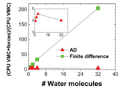
Figure 6: Ratio of CPU time required to compute energies and all force components referenced to the one required for the simple energy calculation within VMC. The calculations refer to 1, 2, 4, and 32 water molecules. The inset is an expansion of the lower part of the plot. Reprinted with permission from Sorella and Capriotti (2010), J. Chem. Phys., published by AIP in 2010.

VI.1 Derivatives with respect to variational parameters

The derivatives of the energy with respect to a given real variational parameter ${{\alpha_{k}}}$ (one complex parameter can be thought to be composed by two real ones, its real and imaginary part, respectively) is represented as a generalized force:

$${f_{k}}=-\frac{{\partial E\left(\alpha\right)}}{{\partial{\alpha_{k}}}}=-\frac{\partial}{{\partial{\alpha_{k}}}}\frac{{\braket{{\Psi_{\alpha}}}{\hat{\mathcal{H}}}{{\Psi_{\alpha}}}}}{{\braket{{\Psi_{\alpha}}}{{\Psi_{\alpha}}}}}.$$ (111)

In variational Monte Carlo, the derivative can be evaluated using $M$ configurations of electron coordinates Becca and Sorella (2017):

$$\begin{split}{f_{k}}&=-2\Re\left[{\sum\limits_{\mathbf{x}}{\frac{{e_{L}^{*}\left({\mathbf{x}}\right)\left({{O_{k}}\left({\mathbf{x}}\right)-{{\bar{O}}_{k}}}\right){{\left|{{\Psi_{\alpha}}\left({\mathbf{x}}\right)}\right|}^{2}}}}{{\sum\nolimits_{\mathbf{x}}{{{\left|{{\Psi_{\alpha}}\left({\mathbf{x}}\right)}\right|}^{2}}}}}}}\right]\\ &\approx-2\Re\left[{\frac{1}{M}\sum\limits_{i=1}^{M}{e_{L}^{*}\left({{{\mathbf{x}}_{i}}}\right)\left({{O_{k}}\left({{{\mathbf{x}}_{i}}}\right)-{{\bar{O}}_{k}}}\right)}}\right],\end{split}$$ (112)

where ${e_{L}\left({{{\mathbf{x}}}}\right)}$ is the local energy, ${O_{k}}\left({\mathbf{x}}\right)$ is the logarithmic derivative of the WF (i.e., ${O_{k}}\left({\mathbf{x}}\right)=\frac{{\partial\ln{\Psi_{\alpha}}\left({\mathbf{x}}\right)}}{{\partial{\alpha_{k}}}}$), and ${{\bar{O}}_{k}}$ is its average over $M$ samples (i.e., ${{\bar{O}}_{k}}=\frac{1}{M}\sum\limits_{i=1}^{M}{{O_{k}}\left({{{\mathbf{x}}_{i}}}\right)}$). In TurboRVB, the logarithmic derivative (${O_{k}}\left({\mathbf{x}}\right)$) is computed very efficiently by using the AAD algoritm. Notice that the derivatives of the local energy are not needed here because the Hamiltonian does not depend on any variational parameter. Instead, these terms are necessary in order to calculate ionic forces (i.e., derivatives of the total energies with respect to atomic postions). If the WF is an exact eigenstate of the hamiltonian, the generalized forces ${f_{k}}$ exactly vanish without statistical errors because the local energy is no longer dependent on ${\mathbf{x}}$. In other words, the derivatives have the zero-variance property and represent therefore the fundamental ingredients for an efficient WF optimization, as described sec. VII.

In practice, during an optimization, the code monitors the variational energy ($E\left(\bm{\alpha}\right)$) and the maximum value of the signal to noise ratio among all the force components, which is denoted as devmax in the code:

$$\verb| devmax |\equiv\max_{k}\left({\left|{\frac{{{f_{k}}}}{{{\sigma_{{f_{k}}}}}}}\right|}\right)$$ (113)

where ${\sigma_{{f_{k}}}}$ represents the estimated error bar of the force ${f_{k}}$. This value is used in TurboRVB as one of the convergence criteria of the optimization. To our experience, after a reasonable number of iterations devmax stabilizes to a value $\leq$ 4.0, when a correct (possibly local) minumum is being approached.

VI.2 Atomic forces

In TurboRVB, a very useful space warp coordinate transformation (SWCT) Sorella and Capriotti (2010) is employed for the calculation of atomic forces. This scheme was introduced several decades ago in Ref. Umrigar, 2009, in order to decrease the statistical errors of forces. The finite-difference expression for ionic forces calculations is:

$${{\mathbf{F}}_{a}}=-\frac{\Delta}{{\Delta{{\mathbf{R}}_{a}}}}E=-\frac{{E\left({{{\mathbf{R}}_{a}}+\Delta{{\mathbf{R}}_{a}}}\right)-E\left({{{\mathbf{R}}_{a}}}\right)}}{{\Delta{{\mathbf{R}}_{a}}}}+O\left({\Delta{{\mathbf{R}}_{a}}}\right).$$ (114)

The SWCT is used to mimic the displacement of charges around the nucleus,

$${{\mathbf{\bar{r}}}_{i}}={{\mathbf{r}}_{i}}+\Delta{{\mathbf{R}}_{a}}{\omega_{a}}\left({{{\mathbf{r}}_{i}}}\right),$$ (115)

$${\omega_{a}}\left({\mathbf{r}}\right)=\frac{{\kappa\left({\left|{{\mathbf{r}}-{{\mathbf{R}}_{a}}}\right|}\right)}}{{\sum\nolimits_{b=1}^{M}{\kappa\left({\left|{{\mathbf{r}}-{{\mathbf{R}}_{b}}}\right|}\right)}}},$$ (116)

where ${\kappa\left(r\right)}$ is a function that decays sufficiently fast for large $r$ because the charges far from the nuclei should not be affected by the SWCT, and $\omega\to 0$, as a consequence of this requirement. It turns out that the originalUmrigar (2009) simple choice $\kappa\left(r\right)=1/{r^{4}}$ works very well and is indeed adopted in TurboRVB.

Starting from the finite-difference expression, one can straightforwardly derive the corresponding differential expression Sorella and Capriotti (2010):

$${{\mathbf{F}}_{a}}=-\left\langle{\frac{d}{{d{{\mathbf{R}}_{a}}}}{e_{L}}}\right\rangle+2\left({\left\langle{{e_{L}}}\right\rangle\left\langle{\frac{d}{{d{{\mathbf{R}}_{a}}}}\ln\left({{{\mathcal{J}}^{\frac{1}{2}}}\Psi}\right)}\right\rangle-\left\langle{{e_{L}}\frac{d}{{d{{\mathbf{R}}_{a}}}}\ln\left({{{\mathcal{J}}^{\frac{1}{2}}}\Psi}\right)}\right\rangle}\right)$$ (117)

where ${\mathcal{J}}$ is the Jacobian of the above transformation, and the brackets indicates a Monte Carlo average over the trial WF. All the terms above can be written by the partial derivatives of the local energy and those of the logarithm of the WF Sorella and Capriotti (2010):

$$\frac{d}{{d{{\mathbf{R}}_{a}}}}{e_{L}}=\frac{\partial}{{\partial{{\mathbf{R}}_{a}}}}{e_{L}}+\sum\limits_{i}{{\omega_{a}}\left({{{\mathbf{r}}_{i}}}\right)\frac{\partial}{{\partial{{\mathbf{r}}_{i}}}}{e_{L}}},$$ (118)

$$\frac{d}{{d{{\mathbf{R}}_{a}}}}\ln\left({{{\mathcal{J}}^{\frac{1}{2}}}\Psi}\right)=\frac{\partial}{{\partial{{\mathbf{R}}_{a}}}}\ln\left(\Psi\right)+\sum\limits_{i}{\left[{{\omega_{a}}\left({{{\mathbf{r}}_{i}}}\right)\frac{\partial}{{\partial{{\mathbf{r}}_{i}}}}\ln\left(\Psi\right)+\frac{1}{2}\frac{\partial}{{\partial{{\mathbf{r}}_{i}}}}{\omega_{a}}\left({{{\mathbf{r}}_{i}}}\right)}\right]}.$$ (119)

In order to evaluate these differential expressions, 6$N$ + 6$N_{\rm at}$ components have to be evaluated, namely, $\left\langle{\frac{\partial}{{\partial{{\mathbf{r}}_{i}}}}{e_{L}}}\right\rangle$, $\left\langle{\frac{\partial}{{\partial{{\mathbf{r}}_{i}}}}\ln\Psi}\right\rangle$, $\left\langle{\frac{\partial}{{\partial{{\mathbf{R}}_{a}}}}\ln{e_{L}}}\right\rangle$, $\left\langle{\frac{\partial}{{\partial{{\mathbf{R}}_{a}}}}\ln\Psi}\right\rangle$ Sorella and Capriotti (2010). These values are very efficiently computed in TurboRVB, by using the aforementioned AAD, that works even in presence of pseudopotentials.

The SWCT significantly decreases the statistical errors, but the forces still have infinite variance properties because $\partial{e_{L}}$ and $\partial\ln\left(\Psi\right)$ diverge in the vicinity of the nodal surfaces. Attaccalite and Sorella Attaccalite and Sorella (2008) developed a reweighting method to address this issue in an unbiased way. Within this scheme, the QMC sampling is not driven by the chosen trial WF ${\Pi_{\text{T}}}\left({\mathbf{x}}\right)=\Psi_{\text{T}}^{2}\left({\mathbf{x}}\right)$, but by a slightly different guiding function ${{\Psi_{\text{G}}}\left({\mathbf{x}}\right)}$ defined by

$${\Psi_{\text{G}}}\left({\mathbf{x}}\right)=\frac{{{R^{\varepsilon}}\left({\mathbf{x}}\right)}}{{R\left({\mathbf{x}}\right)}}{\Psi_{\text{T}}}\left({\mathbf{x}}\right)$$ (120)

where $R\left({\mathbf{x}}\right)$ vanishes more weakly than the trial function does, when the configuration ${\mathbf{x}}$ approaches the nodal surface, whereas ${R^{\varepsilon}}$ is an appropriately chosen regularization of $R$, depending on $\varepsilon$, that never vanishes. In this way, the guiding function is larger when approaching the nodal surface, and this singular region can be more accurately sampled in order to avoid infinite variance problems in the calculation of forces, as it will be shown later. For this purpose, $R\left({\mathbf{x}}\right)$ is defined in a way to vanish as the antisymmetric part of the WF to some power $2\theta_{R}\leq 1$. However, in order to avoid too large fluctuations, a simple relation is used that ${\rm Pf}(G)\simeq{1\over G^{-1}_{i,j}}$, where ${G_{i,j}}$ is the pairing function (Eq.45), here referred to the general AGP case (the other cases straightforwardly follows upon some restriction of the matrix $G$). Indeed, if the Pfaffian goes to zero, most of the matrix elements of the inverse of $G$ diverge inversely proportional to it. Thus the quantity

$$R\left({\mathbf{x}}\right)=\left(S\sum\limits_{i,j}{{{\left|{G_{i,j}}^{-1}\right|}^{2}}}\right)^{-\theta_{R}}$$ (121)

satisfies the requirement without depending explicitly on the full Pfaffian that has fluctuations exponentially large in the number of particles and would lead to an inefficient regularizationAttaccalite and Sorella (2008). Here, we have introduced also the scaling factor $S$, that takes into account that the WF may vanish also when a single particle is going to infinity, and not because it is approaching the nodal surface. In this case, the scaling factor has to vanish in a proper way so as to allow a non-vanishing $R$. In this way, the guiding function can decay sufficiently fast in this limit and can be normalized in an open system. This represents a necessary condition to have a stable simulation, otherwise all electrons will be kicked out at infinity, after a long Markov chain. Therefore, the factor $S$ is chosen to vanish as long as one raw of the pairing function is vanishing, because it is corresponding to an electron going to infinity (all matrix elements containing such electron coordinate have to vanish):

$$S={\rm min}_{i}\sum\limits_{j}|G_{ij}|^{2}.$$ (122)

This definition is also useful, because the regularization proposed is scale-invariant, namely $R\left({\mathbf{x}}\right)$ remains unchanged if $G$ is scaled by an arbitrary constant and therefore is adopted as it is also for bulk systems, and it is particularly important when, in these cases, there exist large regions of almost negligible electronic density.Zen et al. (2013)

After that ${R^{\varepsilon}}\left({\mathbf{x}}\right)$ is defined as:

$${R^{\varepsilon}}\left({\mathbf{x}}\right)={\rm max}\left[R\left({\mathbf{x}}\right),\varepsilon\right]$$ (123)

that is much simpler than the original proposal reported in Ref. Attaccalite and Sorella, 2008. By using the new probability, forces (the HF and the Pulay) can be evaluated with finite variance as:

$${\left\langle{\mathcal{W}\left({\mathbf{x}}\right){\mathbf{F}}\left({\mathbf{x}}\right)}\right\rangle_{{\Pi_{\text{G}}}\left({\mathbf{x}}\right)}}/{\left\langle{\mathcal{W}\left({\mathbf{x}}\right)}\right\rangle_{{\Pi_{\text{G}}}\left({\mathbf{x}}\right)}},$$ (124)

where the $\mathcal{W}\left({\mathbf{x}}\right)$ is the new weight:

$$\mathcal{W}\left({\mathbf{x}}\right)={\left({\Psi_{\text{T}}\left({\mathbf{x}}\right)/{\Psi_{\text{G}}}\left({\mathbf{x}}\right)}\right)^{2}}\equiv\left({R\left({\mathbf{x}}\right)\over{\rm max}\left[R\left({\mathbf{x}}\right),\varepsilon\right]}\right)^{2}$$ (125)

and ${\mathbf{F}}\left({\mathbf{x}}\right)$, according to Eq. 117, indicates the average of an appropriate random variable containing either the derivative of the local energy (the HF contribution) or the product of the local energy and the log derivative of the WF (the Pulay one), both contributions diverging as $\simeq{1\over\delta^{2}}$, where $\delta$ is the distance from the nodal surface. The point is that, since in the vicinity of the nodal surface ${\mathcal{W}\left({\mathbf{x}}\right)}$ is proportional to ${\delta^{4\theta_{R}}}$, whereas the probability vanishes much slower as ${\Pi_{\text{G}}}\left({\mathbf{x}}\right)\simeq\delta^{2-4\theta_{R}}$, the reweighting scheme solves the infinite variance problem for $1/4<\theta_{R}\leq 1/2$ because the random variable ${\mathcal{W}\left({\mathbf{x}}\right)}{\mathbf{F}}\left({\mathbf{x}}\right)$ remains with finite variance. This follows after simple inspection of its integrability in the small $\delta$ region, i.e., $\int d\delta\delta^{4\theta_{R}-2}<\infty$. Thus, both the HF and the Pulay terms can be evaluated with finite variances in the TurboRVB evaluation of atomic forces. In the most recent versions of TurboRVB, the default value of $\theta_{R}$ is taken to be at the middle of the interval of stability, i.e., $\theta_{R}=3/8$, because the value $\theta=1/2$, previously chosenAttaccalite and Sorella (2008), leads to some instability, namely, during the QMC sampling, the nodal surface is approached too much closely, and the determinants or Pfaffians become very ill-conditioned with obvious problems of numerical accuracy. Moreover, the value of $\varepsilon$ is automatically selected during the first steps of the simulation in a way that the average reweighting factor $\left\langle{\mathcal{W}\left({\mathbf{x}}\right)}\right\rangle\simeq 0.8$, that represents empirically an almost optimal setting.

Finally, we remark that this method to compute the energy derivatives with finite variance is applied by default in TurboRVB  even for the optimization of the WF variational parameters, and that a similar approach can be used when computing atomic forces within the LRDMC algorithm.

VII Optimization of WFs

VII.1 Stochastic reconfiguration

Once the energy derivatives can be computed, the most straightforward strategy to optimize a WF is to employ the steepest descent method, where the WF parameters are iteratively updates as follows:

$${\alpha_{k}}\to{\alpha^{\prime}_{k}}={\alpha_{k}}+\delta{\alpha_{k}}$$ (126)

$$\delta{\alpha_{k}}=\Delta{\mathbf{f}_{k}},$$ (127)

where $\Delta$ is a small constant and ${f_{k}}\equiv-\frac{{\partial E}}{{\partial{\alpha_{k}}}}$ is the generalized force already defined in Eq. 111. However, it does not work well when optimizing highly non-linear WF parameters because a small change of a given variational parameter may produce a very different WF, whereas another parameter change may weakly affect the WF. Of course, one can use more sophisticated methods such as the Newton-Raphson method, the conjugate gradient, the quasi-Newton method, but the straightforward implementation of these optimizations do not work efficiently within a stochastic approach like QMC. In order to overcome this difficulty, a more efficient change in the variational parameters has been defined by means of a positive-definite preconditioning matrix ${\bm{\mathcal{S}}}$ and the generalized force vector $\mathbf{f}$:

$${\alpha_{k}}\to{\alpha_{k}}+\Delta\cdot{\left({{{\bm{\mathcal{S}}}^{-1}}{\mathbf{f}}}\right)_{k}},$$ (128)

where the matrix ${\bm{\mathcal{S}}}$ is stochastically evaluated by means of $M$ configuration samples ${\mathbf{x}}=\left\{{{{\mathbf{x}}_{1}},{{\mathbf{x}}_{2}},\ldots{{\mathbf{x}}_{M}}}\right\}$:

$${{\mathcal{S}}_{k,k^{\prime}}}=\left[{\frac{1}{M}\sum\limits_{i=1}^{M}{\left({{O_{k}}\left({{{\mathbf{x}}_{i}}}\right)-{{\bar{O}}_{k}}}\right)^{*}\left({{O_{k^{\prime}}}\left({{{\mathbf{x}}_{i}}}\right)-{{\bar{O}}_{k^{\prime}}}}\right)}}\right],$$ (129)

where ${O_{k}}\left({{{\mathbf{x}}_{i}}}\right)=\frac{{\partial\ln\Psi\left({{{\mathbf{x}}_{i}}}\right)}}{{\partial{\alpha_{k}}}}$ and ${{\bar{O}}_{k}}=\frac{1}{M}\sum\limits_{i=1}^{M}{{O_{k}}\left({{{\mathbf{x}}_{i}}}\right)}$. The resulting approach is the so-called stochastic reconfiguration (SR) method Sorella (1998). Mazzola et al. Mazzola et al. (2012) pointed out that the matrix ${\bm{\mathcal{S}}}$ is essentially a metric for the parameter space, measuring the distance of the underlying normalized WF. Therefore, Eq. 128 is simply the steepest descent in this curved manifold. This observation connects the SR method with the so-called natural gradient method, widely used in the context of deep learning Amari (1998). In this context, for each parameter $\alpha$, $\left({{{\hat{O}}_{k}}-{{\bar{O}}_{k}}}\right)$ and ${{\mathcal{S}}_{k,k^{\prime}}}$ can be interpreted as the score function (i.e., the gradient of the log-likelihood function) and the Fisher information matrix (FIM), respectively, while the WF square ${\left|{\Psi\left({{{\mathbf{x}}}}\right)}\right|^{2}}$ plays the role of the likelihood function. In this sense, the stochastic reconfiguration method is essentially identical to the natural gradient optimization with the FIM that has been intensively used in the machine-learning community.

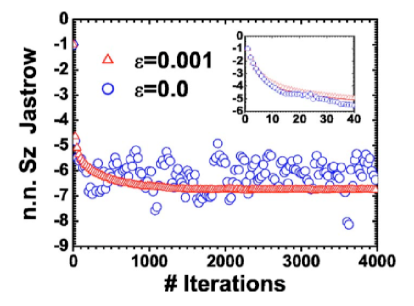
Figure 7: Optimization of the variational WF in the simple one-dimensional Heisenberg model ${\mathcal{H}}=J\sum\nolimits_{i}{{{\vec{S}}_{i}}\cdot{{\vec{S}}_{i+1}}}$ with the standard SR ($\varepsilon$ = 0, open circles) and with the present regularization ($\varepsilon$ = 0.001, open triangles). In the figure, the evolution of the nearest neighbor spin-spin ($S_{z}$) Jastrow parameter is plotted. This figure clearly shows that the SR method with regularization is several orders of magnitude more efficient than the standard SR for determining the variational parameter with a given statistical accuracy. The inset shows the first few iterations. Reprinted with permission from Sorella et al. (2007), J. Chem. Phys., published by AIP in 2007.

The straightforward implementation of the SR method is not stable mainly because the statistical noise sometimes makes the matrix ${\bm{\mathcal{S}}}$ ill-conditioned, which deteriorates the efficiency of the optimization method Sorella et al. (2007). Therefore, in practice, the diagonal elements of the preconditioning matrix ${\mathcal{S}}$ are shifted by a small positive parameter ($\varepsilon$) as:

$${s^{\prime}_{i,i}}={s_{i.i}}(1+\varepsilon).$$ (130)

This modification improves the efficiency of the optimization by several orders of magnitude, as shown in Fig. 7. Finally, the variational parameters are updated as:

$${\alpha_{k}}\to{\alpha_{k}}+\Delta\cdot{\left({{{{\bm{\mathcal{S^{\prime}}}}}^{-1}}{\mathbf{f}}}\right)_{k}}.$$ (131)

In practice, the user should provide two input parameters, namely, $\Delta$ (denoted as tpar in the code input variables) and $\varepsilon$ (denoted as parr).

VII.2 Linear method

In TurboRVB, the state-of-the-art QMC optimization method is also implemented, namely the so-called linear method Sorella (2005); Umrigar et al. (2007); Toulouse and Umrigar (2007). In this scheme, a many-body WF is expanded up the linear order (i.e., considering only the first derivatives for the variational parameters):

$$\ket{{\Psi_{\alpha+\delta\alpha}}}=\ket{{\Psi_{\alpha}}}+\sum\limits_{k=1}{\delta{\alpha_{k}}\frac{{\partial}}{{\partial{\alpha_{k}}}}\ket{{\Psi_{\alpha}}}}\equiv\ket{{\Psi_{0}}}+\sum\limits_{k=1}{\delta{\alpha_{k}}\ket{{\Psi_{k}}}},$$ (132)

where ${{\alpha_{k}}}$ is the $k$-th variational parameter, and ${{\Psi_{k}}\left({\mathbf{x}}\right)}$ is the first derivative with respect to the $k$-th variational parameter. Within this expansion, the expectation value of the energy reads:

$${E_{{\alpha}+{z}}}=\frac{{\sum\nolimits_{k,k^{\prime}=0}^{p}{{z_{k}}^{*}{z_{k^{\prime}}}\braket{{\Psi_{k}}}{\hat{\mathcal{H}}}{{\Psi_{k^{\prime}}}}}}}{{\sum\nolimits_{k,k^{\prime}=0}^{p}{{z_{k}}^{*}{z_{k^{\prime}}}\braket{{\Psi_{k}}}{{\Psi_{k^{\prime}}}}}}}.$$ (133)

In order to obtain the vector ${\mathbf{z}}$ that minimizes this expectation value, one should solve the generalized eigenvalue problem:

$${\bm{\mathcal{H}}\mathbf{z}}=E{\bm{\mathcal{S}}\mathbf{z}},$$ (134)

where ${{\mathcal{H}}_{k,k^{\prime}}}=\braket{{\Psi_{k}}}{\hat{\mathcal{H}}}{{\Psi_{k^{\prime}}}}$ and ${{\mathcal{S}}_{k,k^{\prime}}}=\braket{{\Psi_{k}}}{{\Psi_{k^{\prime}}}}$.

This algorithm is more conveniently implemented in the so-called semi-orthogonal basis Becca and Sorella (2017):

$$\ket{{\Psi_{\alpha+\delta\alpha}}}={z_{0}}\ket{{{\tilde{\Psi}}_{\alpha}}}+\sum\limits_{k=1}{{z_{k}}\left({{{\hat{O}}_{k}}-{{\bar{O}}_{k}}}\right)\ket{{{\tilde{\Psi}}_{\alpha}}}},$$ (135)

where $\ket{{{\tilde{\Psi}}_{\alpha}}}=\ket{{{\Psi_{\alpha}}}}/{{\left\|{{\Psi_{\alpha}}}\right\|}}$, $\braket{x}{{\hat{O_{k}}}}{x^{\prime}}={\delta_{x,x^{\prime}}}{O_{k}}\left({\mathbf{x}}\right)$, ${O_{k}}\left({\mathbf{x}}\right)=\frac{\partial}{{\partial{\alpha_{k}}}}\ln\left|{{\Psi_{\alpha}}\left({\mathbf{x}}\right)}\right|$, and ${{\bar{O}}_{k}}=\braket{{\Psi_{\alpha}}}{{\hat{O_{k}}}}{{\Psi_{\alpha}}}/\braket{{\Psi_{\alpha}}}{{\Psi_{\alpha}}}$. TurboRVB  calculates ${\mathbf{z}}$ by solving the generalized equation (Eq. 134) with the matrices:

$${{\mathcal{H}}_{k,k^{\prime}}}\approx\frac{1}{M}\sum\limits_{i=1}^{M}{\left({{O_{k}}\left({{x_{i}}}\right)-{{\bar{O}}_{k}}}\right)^{*}\frac{{\braket{{x_{i}}}{\hat{\mathcal{H}}\left({\hat{O_{k^{\prime}}}-{{\bar{O}}_{k^{\prime}}}}\right)}{{\Psi_{\alpha}}}}}{\braket{{x_{i}}}{{\Psi_{\alpha}}}}}$$ (136)

$${{\mathcal{S}}_{k,k^{\prime}}}\approx\frac{1}{M}\sum\limits_{i=1}^{M}{\left({{O_{k}}\left({{x_{i}}}\right)-{{\bar{O}}_{k}}}\right)^{*}\left({{O_{k^{\prime}}}\left({{x_{i}}}\right)-{{\bar{O}}_{k^{\prime}}}}\right)}$$ (137)

which can be readily evaluated by a Monte Carlo sampling, using not only the random variables $O_{k}(x_{i})$ necessary for the simpler SR technique, but also the parameter derivatives of the local energy $\partial_{\alpha_{k}}e_{L}(x_{i})$, that can be directly computed by AAD, and thus allow the calculation of the above Hamiltonian matrix elements, by straightforward algebra:

$$\partial_{\alpha_{k}}e_{L}(x_{i})=\partial_{\alpha_{k}}{\langle x_{i}|\hat{\mathcal{H}}|{\Psi_{\alpha}}\rangle\over\langle x_{i}|{\Psi_{\alpha}}\rangle}=\frac{{\braket{{x_{i}}}{\hat{\mathcal{H}}\left({\hat{O_{k^{\prime}}}-{{\bar{O}}_{k^{\prime}}}}\right)}{{\Psi_{\alpha}}}}}{\braket{{x_{i}}}{{\Psi_{\alpha}}}}.$$ (138)

Notice that the code does not always take the eigenvector corresponding to the lowest eigenvalue (that in turn may be also complex, as in the linear method the matrix ${\mathcal{H}}_{k,k^{\prime}}$ is not Hermitian), but takes the one that maximizes ${\left|{{z_{0}}}\right|^{2}}$ (i.e., the coefficient of the zeroth-order term) in order to have the most stable parameter change, namely the updated WF being as close as possible to the old one. Finally, the code updates the variational parameters by using the obtained ${\mathbf{z}}$ and an input parameter $\Delta$ (denoted as tpar) as:

$${\alpha_{k}}\to{\alpha_{k}}+\Delta\cdot{z_{k}}/{z_{0}}$$ (139)

where $\Delta\simeq 1/3$ is the default TurboRVB choice that is much more stable than the original algorithm ($\Delta=1$), but it is approximately $1/3$ slower. The linear method is usually rather unstable for large systems and many parameters, and also, in such cases, each iteration requires a diagonalization of a huge matrix (a task that can be often prohibitive). In TurboRVB, a practical compromise has been devised by using the linear method for a restricted variational space containing up to a maximum number (npbra) of variational parameters with largest signal to noise ratio (optionally larger than parcutpar, see Eq. 113) and/or a number (ncg) of global line parameter directions spanned by the natural gradient ones (e.g., $\Delta$ is one variational parameter of this form in Eq. 131) calculated at the given optimization iteration or the previous closest ones Sorella et al. (2007), optionally neglecting the ones with smaller signal-noise ratio ($<$ parcutmin).

VII.3 Practical Rule

In most optimizations, the number of samplings in VMC is much larger than the number of variational parameters and the optimization is stable and efficient. In the opposite case, the preconditioning matrix ${\mathbf{S}}$ becomes rank-deficient singular; therefore the optimization does not work properly (c.f. the Cramér-Rao inequality). A practical rule is to set the number of samples $M$ such that Becca and Sorella (2017):

$$M\geqslant 5\sim 10\times p,$$ (140)

where $p$ is the number of variational parameters. However, one can also employ very small number of samplings with sufficiently large $\varepsilon$ in the stochastic reconfiguration method because the regularization of the matrix ${\mathbf{S}}$ in Eq. 130 can remove all instabilities as long as $\varepsilon$ is sufficiently large, as in the infinite $\varepsilon$ limit one recovers the very powerful stochastic gradient technique well-known within machine learning. This method seems promising for optimizing even a huge amount of variational parameters and could certainly represent an important development in QMC.

At present, the inversion in Eq. 131 can be done in TurboRVB without storing explicitly the matrixNeuscamman et al. (2012) as the associated linear problem is solved iteratively using conjugate gradients and implicit small matrix-vector operations, optimally distributed within the MPI protocol. Thus the cost of this inversion becomes negligible in the large $\varepsilon$ limit, and linear with the number of variational parameters.

VIII Molecular dynamics

In TurboRVB, several types of ab initio molecular dynamics (MD) have been implemented for both classical and quantum nuclei. The MD is driven by ionic forces $\mathbf{F}=-\bm{\nabla}_{\mathbf{R}}V(\mathbf{R})$, where $\mathbf{F}\equiv\{\mathbf{F}_{1},\ldots,\mathbf{F}_{N}\}$, $\mathbf{R}\equiv\{\mathbf{R}_{1},\ldots,\mathbf{R}_{N}\}$, and the potential energy landscape $V(\mathbf{R})$ is evaluated by VMC, namely

$$V(\mathbf{R})=\frac{\langle\Psi_{\mathbf{R}}|{\hat{\mathcal{H}}}(\mathbf{R})|\Psi_{\mathbf{R}}\rangle}{\langle\Psi_{\mathbf{R}}|\Psi_{\mathbf{R}}\rangle}.$$ (141)

In Eq. 141, $|\Psi_{\mathbf{R}}\rangle$ is the QMC WF that, according to the Born-Oppenheimer (BO) approximation, minimizes the expectation value of ${\mathcal{H}}(\mathbf{R})$ at each ionic position $\mathbf{R}$. The expression for the ionic forces is quite complex. Computing these forces with finite variance and in a fast way, as done in TurboRVB, (Sec. VI.2), is of paramount importance to make a QMC-based MD possible. Moreover, in the QMC framework the evaluation of $V(\mathbf{R})$ and its corresponding force estimators are intrinsically noisy. The statistical noise must be kept under control, if one wants to have an unbiased sampling of the phase space during the propagation of the trajectory. This issue has been solved by resorting to a Langevin type of molecular dynamics in both classical and quantum formulations, where the QMC noise becomes a controlled source of thermalization at the target temperature $T$.

Two types of Langevin dynamics (LD) have been implemented in TurboRVB: the second-order LD, in its classical (Sec. VIII.1) and quantum (Sec. VIII.2) variants, and the first-order LD accelerated by the covariance matrix of QMC forces (Sec. VIII.3).

VIII.1 Second-order Langevin dynamics

The equations of motion of the second-order LD read Attaccalite and Sorella (2008):

$$\dot{\bm{\upsilon}}=-\gamma\left({\mathbf{R}}\right)\cdot{\bm{\upsilon}}+{\mathbf{F}}\left({\mathbf{R}}\right)+{\bm{\eta}}\left(t\right),$$ (142)

$${\mathbf{\dot{R}}}={\bm{\upsilon}},$$ (143)

$$\left\langle{{\eta_{i}}\left(t\right){\eta_{j}}\left({t^{\prime}}\right)}\right\rangle={\mathcal{S}_{i,j}}\left({\mathbf{R}}\right)\delta\left({t-t^{\prime}}\right),$$ (144)

where ${\mathbf{R}}$, ${\bm{\upsilon}}$, ${\mathbf{f}}$, ${\bm{\eta}}$ are the 3$N_{\textrm{at}}$-dimensional vectors representing atomic positions, velocities, deterministic and stochastic forces of $N_{\textrm{at}}$ atoms, written in mass-scaled coordinates:

$$\mathbf{R}_{i} = \mathbf{R}_{i}^{0}\sqrt{m_{i}},$$

$$\mathbf{F}_{i} = \mathbf{F}_{i}^{0}/\sqrt{m_{i}},$$

$$\bm{\eta}_{i} = \bm{\eta}_{i}^{0}\sqrt{m_{i}},$$ (145)

for $i=1,\ldots,N_{\textrm{at}}$. The stochastic forces are related to the friction matrix $\gamma$ through the fluctuation-dissipation theorem, namely:

$$\mathcal{S}\left({\mathbf{R}}\right)=2T\gamma\left({\mathbf{R}}\right),$$ (146)

with the temperature $T$ expressed in atomic units. TurboRVB  exploits the freedom in Eq. 146, by assuming:

$$\mathcal{S}\left({\mathbf{R}}\right)={s_{0}}\mathcal{I}+{\Delta_{0}}{\mathcal{S}^{{\text{QMC}}}}\left({\mathbf{R}}\right)$$ (147)

where ${s_{0}}$ and ${\Delta_{0}}$ are constants, $\mathcal{I}$ is the identity, and ${\mathcal{S}^{{\text{QMC}}}}\left({\mathbf{R}}\right)$ the covariance matrix of QMC forces:

$$\mathcal{S}_{i,j}^{{}^{{\text{QMC}}}}\left({\mathbf{R}}\right)=\Bigl{\langle}{\Bigl{(}{{\mathbf{F}_{i}}\left({\mathbf{R}}\right)-\left\langle{{\mathbf{F}_{i}}\left({\mathbf{R}}\right)}\right\rangle}\Bigr{)}}\Bigr{\rangle}\left\langle{\left({{\mathbf{F}_{j}}\left({\mathbf{R}}\right)-\left\langle{{\mathbf{F}_{j}}\left({\mathbf{R}}\right)}\right\rangle}\right)}\right\rangle.$$ (148)

In the above Equation, $\left\langle\cdots\right\rangle$ refers to the average over the QMC sampling at the given MD step. The friction, a quantity that controls the nuclear sampling efficiency, is, therefore, position-dependent now. Luo et al. have shown that the force covariance matrix $\mathcal{S}_{i,j}^{{}^{{\text{QMC}}}}\left({\mathbf{R}}\right)$ is, within a good approximation, proportional to the dynamical matrix (Fig. 8).

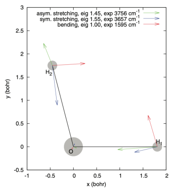
Figure 8: Eigenvectors of the 3 $\times$ 3 correlation matrix of QMC forces $\mathcal{S}^{\text{QMC}}$ in the water monomer. The obtained eigenvectors correspond to the well-known three vibrational modes: bending (red), symmetrical (blue), and asymmetrical (green) stretching. The smaller eigenvalue corresponds to the lowest-frequency vibrational mode. The eigenvalues in the plot are all rescaled by the lowest one. Reprinted with permission from Luo et al. (2014), J. Chem. Phys., published by AIP in 2014.

Therefore, the choice in Eq. 148 realizes the nearly optimal damping of the high-frequency modes. After discretizing Eqs. 142 and 143 in the time interval ${t_{n}}-\tau/2<t<{t_{n}}+\tau/2$, where the index $n$ denotes the time slice ${t_{n}}=n\tau$, with time step $\tau$, and by integrating the above Equations one obtains:

$${{\bm{\upsilon}}_{n+1}}\left(t\right)={e^{-{\gamma_{n}}\tau}}\cdot{{\bm{\upsilon}}_{n}}+{\Gamma_{n}}\left({{{\mathbf{F}}_{n}}+\tilde{\bm{\eta}}}\right)$$ (149)

$${{\mathbf{R}}_{n+1}}={{\mathbf{R}}_{n}}+\tau{{\bm{\upsilon}}_{n+1}},$$ (150)

with ${{\mathbf{F}}_{n}}\equiv{\mathbf{F}}\left({{{\mathbf{R}}_{n}}}\right)$, ${\gamma_{n}}\equiv\gamma\left({{{\mathbf{R}}_{n}}}\right)$,

$${\Gamma_{n}}=\gamma_{n}^{-1}\left({{{I}}-{e^{-{\gamma_{n}}\tau}}}\right),$$ (151)

and

$$\tilde{\bm{\eta}}=\frac{{{\gamma_{n}}}}{{2\sinh\left({{\gamma_{n}}\tau/2}\right)}}\int_{{t_{n}}-\tau/2}^{{t_{n}}+\tau/2}{{e^{-{\gamma_{n}}\left({t-{t_{n}}}\right)}}\cdot{\bm{\eta}}\left(t\right)dt}.$$ (152)

By using Eq. 152, it is easy to show that the correlator defining the discrete noise is given by the following $3N_{\textrm{at}}$ $\times$ $3N_{\textrm{at}}$ matrix:

$$\left\langle{{{\tilde{\eta}}_{i}}{{\tilde{\eta}}_{j}}}\right\rangle\equiv\mathcal{S}^{*}=T\gamma_{n}^{2}\coth\left({{\gamma_{n}}\tau/2}\right).$$ (153)

In this way, $\tilde{\bm{\eta}}$ fulfill the fluctuation-dissipation theorem required by the Langevin thermostat. However, part of this noise is already present in the QMC force evaluation (${{\tilde{\bm{\eta}}}^{{\text{QMC}}}}$), as quantified by Eq. 148. Hence, TurboRVB adds the external random force ${{\tilde{\bm{\eta}}}^{{\text{ext}}}}$, such that ${\tilde{\bm{\eta}}}={{\tilde{\bm{\eta}}}^{{\text{ext}}}}+{{\tilde{\bm{\eta}}}^{{\text{QMC}}}}$. This is generated according to the following correlator:

$$\left\langle{\tilde{\eta}_{i}^{{\text{ext}}}\tilde{\eta}_{j}^{{\text{ext}}}}\right\rangle=\mathcal{S}^{*}-{\mathcal{S}_{\text{QMC}}},$$ (154)

in order to fulfill the original fluctuation-dissipation theorem. Since the correlation matrix in Eq. 154 is positive definite as long as $\tau<{\Delta_{0}}$, the correlated external force can be readily generated by standard algorithms (e.g., the Box-Muller’s method Box and Muller (1958) combined with the matrix diagonalization). This noise correction plays an important role in targeting a stable temperature even in the presence of statistical errors in the QMC forces. The original numerical integration detailed here has been further improved by G. Mazzola and S. Sorella (see the supplementary notes of Ref. Mazzola et al., 2014).

VIII.2 Path integral Ornstein-Uhlenbeck Dynamics

F. Mouhat et. al have recently introduced the nuclear quantum effects into the second-order LD based on a path integral molecular dynamics (PIMD) approach Mouhat et al. (2017), driven by QMC nuclear forces. As a starting point of the Feynman path integral (PI) theory, the quantum partition function $Z=\text{Tr}\left[e^{-\beta{\mathcal{H}}}\right]$ (with $\beta=1/k_{B}T$) can be written asTrotter (1959)

$$Z\simeq\frac{1}{(2\pi\hbar)^{3N_{\textrm{at}}L}}\int\textrm{d}^{N_{\textrm{at}}L}\mathbf{p}\,\textrm{d}^{N_{\textrm{at}}L}\mathbf{q}\,e^{-\tau_{\beta}{\mathcal{H}}_{L}(\mathbf{p},\mathbf{q})},$$ (155)

with $\tau_{\beta}=\beta/L$ denotes the imaginary time step. We have replaced here the true quantum particles by fictitious classical ring polymers, consisting of $L$ replicas (beads) of the system. The beads in these necklaces are connected to each other by harmonic springs, evolving in the imaginary time. Without loss of generality, we can extend the definition of classical vectors to the quantum case, by including all $L$ replicas, such that the resulting vector $\mathbf{q}\equiv\left(\mathbf{R}^{(1)},\ldots,\mathbf{R}^{(i)},\ldots,\mathbf{R}^{(L)}\right)^{T}$ is $3N_{\textrm{at}}L$-dimensional. If interpreted classically, the partition function $Z$ in Eq. 155 describes a system at the effective temperature $LT$. The Hamiltonian ${\mathcal{H}}_{L}$ corresponding to this quantum-to-classical isomorphism reads as

$${\mathcal{H}}_{L}(\mathbf{p},\mathbf{q}) = \sum\limits_{i=1}^{N_{\textrm{at}}}\sum\limits_{j=1}^{L}\left(\frac{1}{2}[\mathbf{p}_{i}^{(j)}]^{2}+\frac{1}{2}\tilde{\omega}_{L}^{2}\left(\mathbf{R}_{i}^{(j)}-\mathbf{R}_{i}^{(j-1)}\right)^{2}\right)$$ (156)

$$+ \sum\limits_{j=1}^{L}V(\mathbf{R}_{1}^{(j)},..,\mathbf{R}_{N_{\textrm{at}}}^{(j)}),$$

written in mass-scaled coordinates Eq. 145, with $\tilde{\omega}_{L}=L/\beta\hbar$, and subjected to the ring boundary condition $\mathbf{R}_{i}^{(0)}\equiv\mathbf{R}_{i}^{(L)}$. The system is thermalized by a Langevin thermostat, such that the related Liouville operator ${\cal L}$ can be written as:

$${\cal L} = \sum_{i=1}^{3N_{\textrm{at}}L}\Biggl{(}{\cal F}_{i}\partial_{p_{i}}+p_{i}\partial_{q_{i}}\Biggr{.}$$ (157)

$$- \Biggl{.}\sum_{j=1}^{3N_{\textrm{at}}L}\gamma_{ij}\biggl{(}\partial_{p_{i}}p_{j}+k_{B}TM\partial_{p_{i}}\partial_{p_{j}}\biggr{)}\Biggr{)}$$

in mass-scaled coordinates, with $\partial_{q_{i}}\equiv\frac{\partial}{\partial_{q_{i}}}$. ${\cal L}$ is built upon the Hamiltonian propagation, driven by the first two terms, and the Langevin thermostat, represented by the last two, deriving from the Fokker-Planck equation. Hereafter in this Section, $i$ and $j$ run over all particles and beads indexed together. In Eq. 157, ${\cal F}_{i}\equiv F^{\textrm{BO}}_{i}+F^{\textrm{harm}}_{i}$ is the total force acting on each replica, comprising the BO (intra-replica) and harmonic contributions (inter-replicas), where $F^{\textrm{BO}}_{i}\equiv-\partial_{q_{i}}{\tilde{V}}$ and ${\tilde{V}}=\sum\limits_{j=1}^{L}V(\mathbf{R}_{1}^{(j)},..,\mathbf{R}_{N_{\textrm{at}}}^{(j)})$.

The quantum-to-classical isomorphism Hamiltonian in Eq. 156 includes very different energy scales. To cope with this, we split the Liouvillian in Eq. 157 into two operators, one containing only the physical (BO) modes, the other depending exclusively on the harmonic modes of the rings. To do so, we first separate the friction matrix into two contributions:

$$\bm{\gamma}=\bm{\gamma}^{\textrm{BO}}+\bm{\gamma}^{\textrm{harm}}.$$ (158)

We can then rewrite the total Liouvillian as the sum of two terms, ${\cal L}={\cal L}^{\textrm{BO}}+{\cal L}^{\textrm{harm}}$, where

$${\cal L}^{\textrm{harm}} = \sum_{i}\Biggl{(}F^{\textrm{harm}}_{i}\partial_{p_{i}}+p_{i}\partial_{q_{i}}\Biggr{.}$$ (159)

$$- \Biggl{.}\sum_{j}\gamma^{\textrm{harm}}_{ij}\biggl{(}\partial_{p_{i}}p_{j}+k_{B}TM\partial_{p_{i}}\partial_{p_{j}}\biggr{)}\Biggr{)},$$

$${\cal L}^{\textrm{BO}} = \sum_{i}\Biggl{(}F^{\textrm{BO}}_{i}\partial_{p_{i}}\Biggr{.}$$ (160)

$$- \Biggl{.}\sum_{j}\gamma^{\textrm{BO}}_{ij}\biggl{(}\partial_{p_{i}}p_{j}+k_{B}TM\partial_{p_{i}}\partial_{p_{j}}\biggr{)}\Biggr{)},$$

in such a way that we can break up the evolution operator via a Trotter factorizationTrotter (1959) to get the following symmetric propagator Tuckerman et al. (1992); Sexton and Weingarten (1992):

$$e^{-{\cal L}\delta t}\simeq e^{-{\cal L}^{\textrm{BO}}\delta t/2}e^{-{\cal L}^{\textrm{harm}}\delta t}e^{-{\cal L}^{\textrm{BO}}\delta t/2}.$$ (161)

The equations of motion corresponding to the propagator in Eq. 161 have been implemented in TurboRVB, where now $F^{\textrm{BO}}_{i}$ can be computed in a QMC framework, and therefore, it can be affected by an intrisic noise, as it was in the classical scheme (Sec. VIII.1).

We note that the equations of motion generated by ${\cal L}^{\textrm{harm}}$ are linear in both $\mathbf{p}$ and $\mathbf{q}$, thus exactly solvable in an analytic closed form. This is because the non-linear BO components of the total force have been put in the ${\cal L}^{\textrm{BO}}$ factor. The dynamics generated by ${\cal L}^{\textrm{harm}}$ is a quantum Ornstein-Uhlenbeck process, which describes the motion of Brownian quantum particles under the influence of friction.

The exact integration of ${\cal L}^{\textrm{harm}}$ without further splitting the Langevin thermostat from the harmonic modes of the rings is a major achievement, which gives the algorithm an enhanced stability and better scaling with respect to the time step size $\tau$ and the number of replica $L$. Moreover, the time step error is significantly smaller than the one of other PILD methodsCeriotti et al. (2010). Thus, this is a key feature of the PI algorithm implemented in TurboRVB. This is also why the implemented method is called path integral Ornstein-Uhlenbeck dynamics (PIOUD).

If we now look at the ${\cal L}^{\textrm{BO}}$ factor in Eq. 161, the corresponding equations of motion are the ones in Eq. (12) of Ref. Luo et al., 2014. Indeed, only the momenta are evolved in ${\cal L}^{\textrm{BO}}$, and the resulting equations are equal to those of the simple classical Langevin algorithm introduced in Ref. Attaccalite and Sorella, 2008, restricted to $\mathbf{p}$, which in the present case is a $3N_{\textrm{at}}L$-dimensional vector. As in the classical second-order QMC-driven LD, the QMC noise affecting the BO forces is controlled thanks to the friction $\bm{\gamma}^{\textrm{BO}}$ and the fluctuation-dissipation theorem. A noise reduction scheme similar to the one described in Eqs. 153 and 154 is also applied in this case, yielding a thermalization towards a steady temperature ensemble even for quantum particles.

We refer the interested reader to Ref. Mouhat et al., 2017, where we report a detailed description of the PIOUD algorithm and the integrated equations of motion.

VIII.3 First-order Langevin dynamics

TurboRVB also features an accelerated first-order dynamics to sample the (classical) ionic canonical distribution. This molecular dynamics scheme has been introduced recently by G. Mazzola and S. Sorella Mazzola and Sorella (2017). Here, the ions formally undergo the following dynamics

$${\mathbf{\dot{R}}}={\mathcal{S}^{-1}}\left({\mathbf{R}}\right)\cdot{\mathbf{F}}\left({\mathbf{R}}\right)+{\bm{\eta}}$$ (162)

$$\left\langle{{\eta_{i}}{\eta_{j}}}\right\rangle=2T\delta\left({t-t^{\prime}}\right)\mathcal{S}_{i,j}^{-1}\left({\mathbf{R}}\right)$$ (163)

where $T$ is the temperature, ${\mathbf{F}}\left({\mathbf{R}}\right)$ and ${\bm{\eta}}$ are the deterministic and stochastic forces, $\mathcal{S}$ is the covariance matrix of the QMC forces as introduced in Eq. 148. This dynamics generalizes the Newton method, which is valid for structural relaxation, to finite-temperature.

Indeed, the use of the matrix $\mathcal{S}$, which is empirically proportional to the Hessian matrix, can drastically decrease the autocorrelation time of the Markov chain. In other words, this metric plays an important role in treating the different time scales of a given system. In this way, one can still use a quite large integration time step $\tau$, which is beneficial in reducing the autocorrelation time of quantities that depend on slowly varying degrees of freedom (e.g., molecular diffusion), without introducing any bias in the sampling.

Discretization of Eq. 162 for a finite time step $\tau$ at finite temperature is rather involved and has been described in the Ref. Mazzola and Sorella, 2017, and reads

$$\begin{split}{\mathbf{R}}\left({t+\tau}\right)&={\mathbf{R}}\left(t\right)+\sqrt{2T\tau}\cdot{\mathbf{z}}\left(t\right)+\tau{{\mathcal{S}}^{-1}}\left({\mathbf{R}}\right){\mathbf{F}}\left({\mathbf{R}}\right)\\ &-{{\mathcal{S}}^{-1}}\left({\mathbf{R}}\right)\left({\frac{{{\mathcal{S}}\left({{\mathbf{R}}\left({t-\tau}\right)}\right)-{\mathcal{S}}\left({\mathbf{R}}\right)}}{2}}\right)\left({{\mathbf{R}}\left({t-\tau}\right)-{\mathbf{R}}\left(t\right)}\right),\end{split}$$ (164)

with

$$\left\langle{{z_{i}}\left(t\right){z_{j}}\left(t\right)}\right\rangle=\mathcal{S}_{i,j}^{-1}\left({{\mathbf{R}}\left(t\right)}\right).$$ (165)

As the effective temperature depends on the finite integration time, the convergence to the target temperature $T_{\text{target}}$ for $\tau\to 0$ can be improved by a renormalization of the temperature $T$ used in the simulation, namely by using the above equations with an appropriate choice of $T$:

$$T=T_{\text{target}}~{}(1-a\tau),$$ (166)

where $a=1/2$ in the case of the harmonic potential leads to the exact result for any discretization time $\tau$, as long as $S$ is the exact elastic matrix. In the general case, the parameter $a$ should be tuned to speed up convergence to the $\tau\to 0$ limit. Conversely, the target temperature of the simulation can be measured a posteriori, as it is often done in the case of second-order Langevin dynamics, by measuring the average squared velocities of the particles.

The accelerated first-order Langevin dynamics has been successfully employed in the most recent studies of dense liquid hydrogen, providing equilibrated simulations even close to phase transitions Mazzola and Sorella (2017); Mazzola et al. (2018). Moreover, nuclear quantum effects can also be computed within this first-order LD, in exactly the same way as it was implemented for the second-order case discussed in sec. VIII.2. However, so far, it is not clear which method is more efficient and further studies are also necessary to clarify what is the optimal choice of the acceleration matrix $S(\mathbf{R})$ within the QMC framework.

Table 2: Main modules in TurboRVB.

Module	Description
makefort10.x	Generates a JAGP WF from a given basis set and structure.
assembling_pseudo.x	Prepares pseudo potentials.
convertfort10mol.x	Adds molecular orbitals. If the number of molecular orbitals is equal to (larger than) half the number of electrons in a system, the resultant WF is the JSD (JAGPn).
convertfort10.x	Converts a wave function type (fort.10_in), i.e., JSD/JAGP/JAGPn/JPf/JPfn, to another one with a different type (fort.10_out). The output (fort.10_new) is as close as possible to the input and may also include an optimal contracted (hybrid) basis set.
convertfortpfaff.x	Converts a JAGP WF to a JPf one.
prep.x	Performs a DFT calculation.
turborvb.x	Performs VMC optimization, VMC evaluation, LRDMC, structural optimization and molecular dynamics.
readforward.x	Performs correlated samplings, and calculates various physical properties.

IX Implementation and operations

Table 2 shows the main modules implemented in TurboRVB and a brief description of their functionalities. All programs reported in Table 2 are coded in Fortran90. The flow-chart of a typical QMC calculation (see Fig. 1) is detailed as follows: starting from the geometry and the chemical composition, the user first chooses the basis set for both Jastrow and antisymmetric factors, and generates a JAGP-type ansatz using makefort10.x (fort.10 is the wave function filename in TurboRVB).

The antisymmetric part of the WF is initially determined at the DFT mean-field level. Since the DFT calculation is based on a single Slater determinant, the generated JAGP WF should be converted to a JSD one. This is performed by the convertfort10mol.x module, which adds $M$ molecular orbitals to the WF, where $M$ = $N^{\uparrow}$. The DFT molecular orbitals are then used to construct the initial trial WF for subsequent QMC calculations. In QMC, the user can choose to work with five different ansätze, namely, JSD, JAGP, JAGPn, JPfn, and JPf. The initial antisymmetric part of the JSD and JAGPn wave functions can be directly obtained from the DFT orbitals. In the JSD case, only the occupied orbitals are imported, while in the JAGPn WF also the unoccupied orbitals will be used in the geminal expansion, up to the $n$-th orbital. Another possibility is to employ a JAGP ansatz. In that case, one has to convert the initial JSD trial WF obtained by DFT to the JAGP one using convertfort10.x.

JAGPn can also be obtained by applying convertfort10mol.x to a previously determined JAGP ansatz. Analogously, a JPf WF can be converted from a JAGP WF using convertpfaff.x. JPfn can be obtained by applying convertfort10mol.x to the JPf ansatz. These conversions can be done either before or after a QMC optimization. The possibilities for ansatz conversion are schematically drawn in Fig. 4.

After the initial determination of the antisymmetric part of the WF, one performs the WF optimization at the VMC level. This is an important step used to determine the best variational parameters of the Jastrow factor at fixed determinant, or to fully relax the WF by optimizing both Jastrow and determinant parameters.

Finally, the user can proceed to VMC and LRDMC calculations using the optimized WF. In LRDMC, in order to remove the lattice discretization error, it is better to repeat the calculations with several lattice spaces $a$, and to extrapolate the results with a quartic function $E\left(a\right)={E_{0}}+{k_{1}}{a^{2}}+{k_{2}}{a^{4}}$, where ${E_{0}}$ is the extrapolated ($a\to 0$) energy.

The python tool Turbo-Genius makes all the above steps more straightforward, as discussed later.

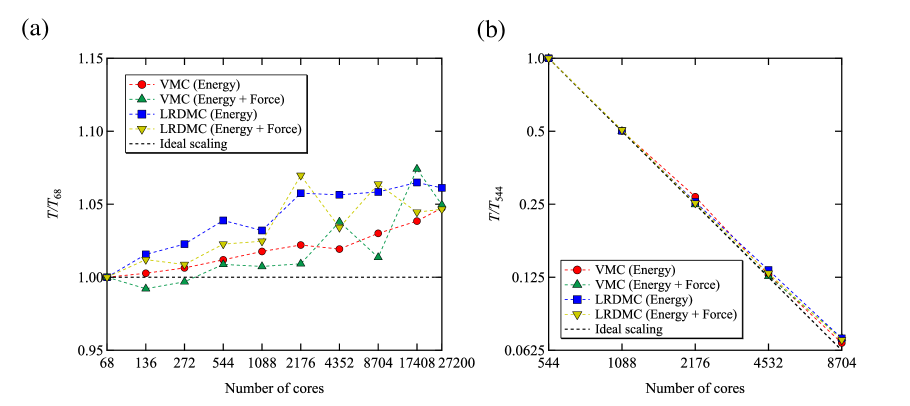
Figure 9: (a) The weak and (b) strong scalings of TurboRVB. The benchmarks were measured using the conventional 2 $\times$ 2 $\times$ 2 diamond with the ccECP pseudo potential (256 electrons in the simulation cell) on Marconi KNL nodes (Cineca supercomputer/SCAI).

X Parallelization and benchmarks

TurboRVB  has been parallelized using the MPI and OpenMP libraries, also supporting the hybrid MPI/OpenMP protocol. As well known, the QMC algorithm is readily parallelized by employing many independent random walks (called walkers), initialized with different seeds for random number generators. Fig. 9 shows the strong and the weak scaling performances of TurboRVB, which are compared with the ideal scaling. The benchmarks have been measured using the conventional 2 $\times$ 2 $\times$ 2 diamond supercell containing 64 carbon atoms for a simulation with 256 electrons on Marconi KNL nodes (Cineca supercomputer/SCAI, Intel Xeon Phi 7250 CPU, 1.40 GHz, 68 cores per node without hyperthreading). For the weak scaling case, we set the number of walkers $M$ to the minimum possible one (one walker per core) and increased the number of cores from 68 (one node) to 27200 (400 nodes). On the other hand, for the strong scaling case, we fixed the number of walkers $M$ = 2176 and increased the number of cores from 544 (8 nodes) to 8704 (128 nodes) with the hybrid MPI/OpenMP protocol (the number of openMP threads was set to four). For both cases, the performances are excellent, because all techniques are off from the ideal scaling by $\sim$ 5% at worst in all cases performed here. At present, the code does not support the use of GPU accelerators. This feature is currently under development.

XI Postprocessing

XI.1 Correlated Samplings

A very efficient and easy-to-use correlated sampling technique has been implemented in TurboRVB. This is very useful in evaluating total energy differences between two very similar WFs. One of its practical sides is to investigate whether a conversion of a WF (e.g., JSD $\to$ JAGP) has been successful. A user should run a short VMC calculation using one of the two mentioned WFs, during which the walkers’ history is stored in an appropriate scratch area (turborvb.scratch). After that, a second run should be executed (by using the readforward.x module) to determine at the end the correlated energy difference and the overlap between the two WFs. Correlated samplings for LRDMC or for the difference in other quantities, e.g., forces, have not been implemented yet. The latter could be very important for the frozen phonon calculation based on the ionic force difference method, which represents a possible subject of research.

XI.2 Physical properties

TurboRVB  enables us to calculate various properties using the optimized many-body WF at both the VMC and LRDMC levels by averaging local observables and applying the forward walking technique Becca and Sorella (2017). The observables presently available in the readforward.x module can be categorized as follows: $\rm(\hskip 1.79993pti\hskip 1.79993pt)$ Charge density [$\rho\left({\mathbf{r}}\right)={\rho^{\uparrow}}\left({\mathbf{r}}\right)+{\rho^{\downarrow}}\left({\mathbf{r}}\right)$] and spin density [${\rho^{\sigma}}\left({\mathbf{r}}\right)=({\rho^{\uparrow}}\left({\mathbf{r}}\right)-{\rho^{\downarrow}}\left({\mathbf{r}}\right))/2$], fundamental properties obtained by a stochastic evaluation of multi-dimensional integrals, involving the many-body WF and improved estimators, such as those proposed by Assaraf, Caffarel, and Scemama Assaraf et al. (2007). Fig. 10 shows the charge density of the square four hydrogen (H₄) depicted by C. Genovese et al. $\rm(\hskip 0.80002ptii\hskip 0.80002pt)$ Electronic correlation functions, such as the charge-charge and spin-spin structure factors, useful to study the critical behavior close to a phase transition, or the physical properties of a given phase. $\rm(iii)$ The expectation values of the spin component along the quantization axis (${S_{z}}$) and the spin square (${S^{2}}$) operators inside a sphere centered on each atom Genovese et al. (2019a, 2020), whose radius can be specified by the user. $\rm(iv)$ The Berry phase: ${z_{\alpha}}=\braket{\Psi}{{e^{i\left({2\pi/L^{\alpha}}\right)\sum\nolimits_{i=1}^{N}{r_{i}^{\alpha}}}}}{\Psi}$, where the complex polarization is computed for the $\alpha=\{x,y,z\}$ component ${r_{i}^{\alpha}}$ of the position vector $\mathbf{r}_{i}$, and $L^{\alpha}$ is the supercell length in the same direction $\alpha$ Stella et al. (2011). This property can be used to characterize the metal-insulator transition based on the many-body WF, as it has been done in the one-dimensional hydrogen chain by L. Stella et al. (Fig. 11).

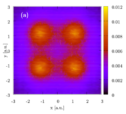
Figure 10: The $xy$-plane charge density of the square four hydrogen (H₄), calculated using a JAGP WF. Reprinted with permission from Genovese et al. (2019b), J. Chem. Phys., published by AIP in 2019.

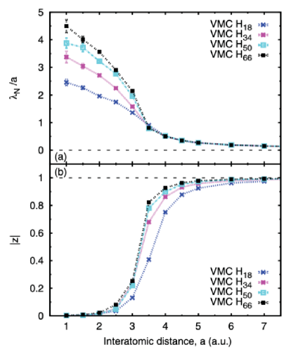
Figure 11: (a) Electronic localization length ${\lambda}_{N}$ divided by the interatomic distance $a$ as a function of $a$, for the one-dimensional hydrogen chain, where ${\lambda}_{N}$ is defined as ${\lambda_{N}}=\left({L/2\pi}\right)\sqrt{-\ln{{\left|{{z_{N}}}\right|}^{2}}/N}$, $N$ is the number of electrons (hydrogen atoms), and $L$ is the length of the simulation cell along to the one dimensional chain. (b) Modulus of the complex polarization $z_{N}$ as a function of the interatomic distance of the hydrogen atoms. According to the previous works Resta and Sorella (1999); Capello et al. (2005), in the thermodynamic limit ($N\to 0$), a metal can be characterized by a vanishing modulus of the complex polarization ($\left|{{z_{N}}}\right|\to 0$, ${\lambda_{N}}\to+\infty$), while it becomes unity in the insulating case ($\left|{{z_{N}}}\right|\to 1$, ${\lambda_{N}}\to 0$). Thus, one can discuss the metal-insulator transition. Reprinted with permission from Stella et al. (2011), Phys. Rev. B, published by APS in 2011.

XII Applications

Since the start of the TurboRVB project in 2003 by M. Casula and S. Sorella Casula and Sorella (2003), the code has been applied to study atomic species, molecular systems, and various materials, including challenging systems such as large complexes, surfaces, liquids, and so on. Here, we provide a brief review of the applications done so far.

XII.1 Molecular systems

TurboRVB  has been employed to study the properties of several molecular systems, including small diatomic systems (such as Li₂, Casula et al. (2004) Be₂, Marchi et al. (2009); Sorella and Zen (2014) B₂, Marchi et al. (2009) C₂, Marchi et al. (2009); Genovese et al. (2019a) N₂, Marchi et al. (2009) O₂, Casula et al. (2004); Marchi et al. (2009); Zen et al. (2014b); Genovese et al. (2020), F₂, Marchi et al. (2009) Na₂, Nakano et al. (2019) LiF, Marchi et al. (2009) CN, Marchi et al. (2009) Fe₂ Casula et al. (2009)), reactive oxygen species (singlet O₂, O${}_{2}^{-}$, OH^∙, OH^-, NO^∙, NO^-, HOO^∙, HOO^-, cis and trans HOOO^∙), Zen et al. (2014b) aromatic molecules (benzeneCasula et al. (2004, 2005b), oligoacene seriesDupuy and Casula (2018), see section XII.4), the water molecule,Casula et al. (2004); Zen et al. (2013) dimerSterpone et al. (2008); Zen et al. (2015b) and hexamer clusters,Zen et al. (2015b) the Zundel ion (H₅O${}_{2}^{+}$) Dagrada et al. (2014); Mouhat et al. (2017), H₂S, SO₂, NH₃, PH₃,Luo et al. (2014) and others. Most of the studies report both variational and FN diffusion Monte Carlo results, and several of the WF ansätze available in TurboRVB are tested. Often, it is shown that quite good results are already obtained at the variational level, and the FN DMC further improves the accuracy of the outcomes. For instance, see the case of the sodium dimer in Fig. 12.

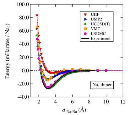
Figure 12: PES of the sodium dimer. The dashed lines show the obtained Murrell-Sorbie function. The error bars are within the markers. The obtained LRDMC PES agrees with the CCSD(T) and experimental ones. Reprinted with permission from Nakano et al. (2019), J. Chem. Theory Comput., published by ACS in 2019.

Table 3 and Fig. 13 report the binding energies for the molecular dimers of the first-row atoms, evaluated using LRDMC with the JSD, JAGP, or JPf WF ansätze as guiding functions. Some of them are close or reach the chemical accuracy (i.e., 1 kcal/mol or $\sim$0.04 eV). A systematic improvement going from the JSD $\to$ JAGP $\to$ JPf can be appreciated. It follows from the employment of a more flexible parametrization of the WF, which improves both the variational energy and the quality of the nodes. However, the improvement given by the JPf ansatz over JAGP and JSD is even more fundamental than what Table 3 and Fig. 13 indicate, where the reported binding energies are evaluated as the difference between the energy of the molecule and twice the energy of the atom. This evaluation does not highlight that JPf is a size-consistent ansatz, while both the JSD and the JAGP have a size-consistency issue with most of the molecules considered. Let us consider the oxygen molecule as an example: the O₂ ground state is a spin triplet (${}^{3}\Sigma_{g}^{-}$) which, in both JSD and JAGP, can be described using two unpaired electrons with the same spin. However, as we take the oxygen atoms far apart (say, the O-O system), they should both be in the ground state for the oxygen atom, which is also a spin triplet (${}^{3}P$). Neither JSD nor JAGP have the flexibility to describe the O-O system by the same WF parametrization used for the O₂, thus $E_{\text{O-O}}>2E_{\text{O}}$. In contrast, JPf has the flexibility to describe the dissociation limit correctly, so $E_{\text{O-O}}^{\text{JPf}}=2E_{\text{O}}^{\text{JPf}}$. Fig. 14 shows that JPf is indeed able to provide a reliable dissociation curve of the oxygen molecule, whereas JSD and JAGP are reliable only in proximity of the minimum. Notice that the FN projection scheme alleviates in part the limitations of the underlying ansatz, as both JSD and JAGP have a smaller size-inconsistency at the LRDMC than at the VMC level, but the correction is incomplete and the inconsistency is sizable ($>1$ eV) for all but the JPf ansatz. Therefore, in general, JPf will yield a better description of the overall potential energy surface (PES), including binding energies, vibrational frequencies, zero-point motion, transition states, and so on.

Table 3: Binding energy of the first-row dimers calculated by TurboRVB with LRDMC and different types of ansätze as a guiding function (GF), at the experimental bond length (see. Ref. Toulouse and Umrigar, 2008). Js denotes the symmetric (i.e., spin-independent) Jastrow factor. LRDMC calculations are performed with several lattice spaces $a$ and extrapolated for $a\to 0$. The spin-orbit coupling and the zero point energies Marchi et al. (2009) are not included in these evaluations.

Binding energy (eV)	Li2	Be2	B2	C2	N2	O2	F2
LRDMC (GF=JSD)	0.976(6)	0.144(7)	2.83(1)	5.74(2)	9.67(1)	4.94(3)	1.27(1)
LRDMC (GF=JsAGPs)	0.9812(12)	-0.0270(12)	2.66(1)	6.01(1)	9.91(1)	5.06(2)	1.56(1)
LRDMC (GF=JPf)	1.0580(12)	0.0304(22)	2.75(1)	6.31(1)	9.97(1)	5.127(6)	1.64(1)
Est. exact	1.06(4)	0.1153(3)	2.91(6)	6.43(2)	9.902(3)	5.233(3)	1.693(5)

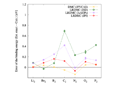
Figure 13: Binding energies of the first-row dimers at their experimental bond length (see. Table. 3). The vertical axis shows the difference between the LRDMC and the estimated exact binding energies. The results obtained from the DMC using a Jastrow correlated full-valence-CAS as trial WF (DMC(JFVCAS)) are taken from Ref. Toulouse and Umrigar, 2008.

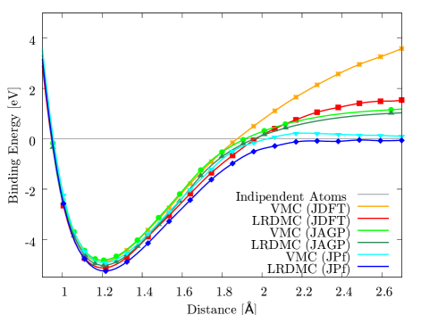
Figure 14: O₂ dissociation curve as obtained with TurboRVB  at the variational (VMC) and fixed-node projected (LRDMC) levels of theory and using JSD with DFT orbitals (JDFT), JAGP and JPf WF ansätze.

The applications of TurboRVB are not limited to single point evaluations. As discussed in Sec. VI, a distintive feature of TurboRVB  among most QMC codes is the efficent evaluation of atomic forces. This capability has been extensively exploited to investigate several properties of the PES, such as vibrational properties, and to perform geometry optimizations and molecular dynamics simulations at finite temperature. It is important to remember that QMC atomic forces are, as the QMC energy, affected by a stochastic error. In a first attemptZen et al. (2012) to evaluate vibrational frequencies of a triatomic molecule (namely, water), a grid of points close to the guessed minimum geometry was used to evaluate energy and forces. The results were used to fit the PES around the minimum with a truncated Taylor expansion, yielding evaluations of the structural minimum and of both the harmonic and anharmonic vibrational frequencies (using the second-order perturbation theory). It was observed that the inclusion of the estimates of forces reduces the stochastic error on the vibrational frequencies by around an order of magnitude with respect to the fit using only the energy evaluations (on the same grid and using the same sampling size on each single point evaluation). This corresponds to about a 25 times larger speedup. Moreover, it was observed that the optimal grid is a tradeoff between maximizing the precision on the vibrational properties and minimizing the errors on the fit. A systematic study of the quality of the variational WF ansätze in relation to the vibrational (and other) properties of the water molecule is reported in Zen et al. (2013). Afterward, Y. Luo et al.Luo et al. (2014); Luo and Sorella (2015) automated the process of finding the optimal grid by performing fits on samples generated by a finite temperature molecular dynamics, and applied the approach to H₂O, H₂S, SO₂, NH₃, and PH₃. The obtained vibrational frequencies are in good agreement with the experimental values.

Zen et al. (2015b) applied the second-order LD to study the structural properties of liquid water. They obtained radial distribution functions in good agreement with recent neutron scattering and X-ray experiments, especially for the position of the oxygen-oxygen peak, which is very sensitive to the quality of the water description and, in particular to the inclusion of dispersive vdW forces. This is a stringent test for ab initio approaches as the shape of the peak can be directly compared with neutron scattering data.

F. Mouhat et al. developed a path integral LD formalism particularly suited for QMC and applied it to the Zundel ion (H₅O${}_{2}^{+}$), with the aim of studying nuclear quantum effectsMouhat et al. (2017). The outcome of their study shows how essential is the inclusion of nuclear quantum effects to properly deal with proton transfer in water and aqueous systems, even at room temperature.

XII.2 Weakly bonded systems and non-covalent interactions

An important application for QMC is the description of systems interacting through weak van der Waals (vdW) dispersive interactions, which are fundamental in supramolecular chemistry, layered and porous materials, molecular crystals, adsorption of molecules on surfaces, and so on. vdW interactions play a major role also in non-covalent intra-molecular bonds, which result from the interplay of forces of different nature, including electrostatic contributions. An accurate evaluation of the overall strength of these non-covalent bonds requires each component of the interaction to be modeled correctly. This is a big challenge for all ab initio approaches, and only a few methods prove reliable. QMC and CCSD(T) are considered to yield very accurate estimates, and there is a general agreement among the predictions from these two theories. Thus, they are typically used to produce benchmark values. Traditionally, mean-field schemes have difficulties in describing dispersive interactions, because they arise from non-local electron correlations, completely missed by local density functionals. However, in the context of DFT, there has been an intensive effort in developing new exchange correlation functionals Grimme et al. (2010) to include vdW interactions. This is usually done in a semi-empirical way, often building on the benchmark provided by CCSD(T) or QMC.

The non-covalent interactions are typically a tiny fraction of the total energy of a compound. Similarly to the cases discussed in Sec. XII.1, also in the evaluation of weak interactions it is important to use a size-consistent approach. However, very often, the molecules form a closed shell, and most of the times the intermolecular interactions are among fragments having zero spin. In this case, a single Slater determinant is a size-consistent ansatz, and so is the JSD. The AGP (without Jastrow) is not size-consistent, due to the presence of unphysical charge fluctuations Sorella et al. (2007); Goetz and Neuscamman (2017), but a very flexible (i.e., large) Jastrow factor allows damping the charge fluctuations and recovering the size-consistency in the JAGP. This is of course true also in a subsequent FN-DMC projection, which is indeed equivalent to applying an infinitely flexible Jastrow factor to the trial WF. At the variational level, the JSD ansatz occasionally leads to better results than the JAGP. Even though JAGP leads to a lower total energy, it is indeed difficult to use a Jastrow factor large enough to damp any charge fluctuation. So, there is a worse error cancellation when energy differences are considered in JAGP. This was observed, for instance, in the water dimer,Zen et al. (2015b) although at the FN level JSD and JAGP lead to the same binding energy. It should also be considered that in the widely used DMC schemeUmrigar et al. (1993) a size-consistency issue was present in any simulation with finite time step $\tau$, until the modification of the “standard” algorithm has been introduced by Zen et al. (2016a), whose solution removes almost completely the size-consistency error. At variance with DMC, the LRDMC algorithm does not suffer from this bias, and it is always size consistent.

The DMC scheme is commonly used to project a single Slater determinant WF where only the Jastrow factor has been optimized, while the antisymmetric part is filled with DFT orbitalsNemec et al. (2010) (JDFT). The resulting FN energy is usually biased by the nodal surface, kept frozen from previous DFT or lower level mean-field calculations. Optimizing the Jastrow factor and determinant together, which is routinely done in TurboRVB, improves significantly the total energy. However, in the evaluation of non-covalent interactions, there is not yet a clearcut indication of the advantage of the full optimization over JDFT. This is due to the fact that the error cancellation plays a major role. Indeed, it is expected that, for non-covalent interactions, JDFT has almost the same bias in the interacting and non-interacting systems. When pseudopotentials are used, DLAZen et al. (2019) can be used to remove any bias given by the Jastrow optimization.

TurboRVB with JDFT, JSD, and JAGP guiding functions has been applied to several interesting systems, such as molecular hydrogen adsorbed on benzene Beaudet et al. (2008), benzene dimers Sorella et al. (2007), graphite layers Spanu et al. (2009), water or methanol molecules adsorbed on a clay surface (see Fig. 15) Zen et al. (2016b), metalic clusters Nissenbaum et al. (2009), and to evaluate the cohesive energies of B₂O₃ polymorphs Ferlat et al. (2019).

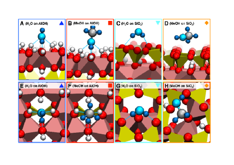
Figure 15: Adsorption of water and methanol on the hydroxyl-terminated and the silicate-terminated faces of kaolinite (side view in first row, top view in second row). The adsorbed molecule on kaolinite is depicted in cyan and gray and the H-bonds are represented by the blue dashed lines. Reprinted with permission from Zen et al. (2016b), J. Phys. Chem. C, published by ACS in 2016.

XII.3 Strongly correlated and superconducting materials

Another important QMC application is the study of strongly correlated materials, that represents a challenge for any theoretical method, because in several cases a fully consistent description remains, so far, elusive. In this context, QMC methods have been widely used for solving, as accurately as possible, strongly correlated lattice Hamiltonians, like, for instance, the Hubbard model. Real-space ab initio QMC methods could fill the gap between realistic Hamiltonians and lattice models, by providing an accuracy similar to the one reached in lattice Hamiltonians, while keeping the complexity of real materials. TurboRVB  has been originally conceived in this perspective, with the idea that one of the most flexible WF ansätze tested on correlated lattice modelsCalandra et al. (1998); Capriotti et al. (1999); Becca et al. (2000); Capriotti et al. (2001); Sorella et al. (2002), namely the generalized version of the resonating valence bond (RVB) WF, could be translated into a successful variational WF for ab initio systems. One of the most appealing features of the RVB WF is that it allows several broken-symmetry phases, such as antiferromagnetic insulators and superconductors, which are present - and sometimes coexisting - in the extremely rich phase diagrams of strongly correlated materials. As introduced in Sec. III, the RVB WF employed in TurboRVB  takes the static and dynamic correlation effects into consideration beyond the commonly used Jastrow-Slater determinant (JSD) WF. Therefore, the code is expected to describe strongly correlated systems more accurately. In particular, among the various families of correlated WFs which go beyond the simplest JSD form, the JAGP/JPfaffian families are very suitable to describe extended systems, as they keep a compact and still strongly correlated form even in the thermodynamic limit. Indeed, as detailed in Sec. III, the AGP part is the particle number conserving version of the BCS WF. In the same way, the JAGP variational form can be seen as an efficient formulation of a RVB WF. Thus, superconducting materials including cuprates Bednorz and Müller (1986) and iron pnictides and selenides Kamihara et al. (2008) are prominent applications of the JAGP/RVB WFs. By running extensive VMC calculations for CaCuO₂, a parent compound of cuprate high-temperature superconductors, M. Marchi et al. validated the JAGP description by correctly finding the expected $d$-wave symmetry of the pairing function Marchi et al. (2011). M. Casula and S. Sorella applied the RVB WF to FeSe, one of the iron-based high-temperature superconductors Casula and Sorella (2013), whose electronic structure and pairing mechanism have been unclear and intensively debated. They determined the symmetry of the superconducting order parameter and the size of its gap entirely from first principles, by analyzing the AGP pairing function (Fig. 16). B. Busemeyer et al. applied DMC and LRDMC to study the structural and magnetic properties of the normal state of FeSe under pressure, and reported that collinear spin configurations are energetically more favorable than other spin patterns, such as ferromagnetic, checkerboard, and staggered dimer, over a large range of pressures Busemeyer et al. (2016).

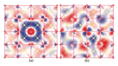
Figure 16: (a) Even-even and (b) odd-even components of the AGP pairing function of FeSe at 0 GPa obtained by VMC calculations, where even and odd refer to the parities of the orbitals to the reflection through the Fe plane. The contour plots show $\Phi\left({{{\mathbf{R}}_{{\text{center}}}},{\mathbf{r}}}\right)$ with ${{\mathbf{R}}_{{\text{center}}}}$ set to be the iron lattice site at the center of the supercell, while ${\mathbf{r}}$ spans the plane defined by the 4 $\times$ 4 lattice. Red (yellow) balls are iron (selenium) sites. Arbitrary units of blue (red) intensity indicate negative (positive) regions with corresponding magnitude. Reprinted with permission from Casula and Sorella (2013) Phys. Rev. B, published by APS in 2013.

XII.4 Aromatic and honeycomb lattice compounds

Aromatic compounds are also successful examples of the RVB theory, because they are characterized by resonating C-C bonds that can be efficiently represented by antisymmetrized singlet pairing functions (i.e., antisymmetrized product of geminals, or AGP). M. Casula et al. applied the AGP WF combined with a Jastrow factor to the simplest aromatic compound, that is, the benzene molecule (C₆H₆) for the first time Casula et al. (2004, 2005b). They reported that the inclusion of the resonance between the two possible Kekulé states significantly lowers the VMC energy compared with the one obtained by a single Kekulé WF. They also showed the importance of adding a three-body Jastrow factor to improve the AGP description, just in the spirit of the RVB framework. By selectively switching on the intersite resonances, they proved that the Dewar contributions (i.e., including the third nearest neighbor carbons) improves the description of the resonating valence bond. C. Genovese et al. have applied a more general AGP WF, i.e., the Pfaffian, to the benzene molecule Genovese et al. (2020). They reported that the obtained atomization energies are reasonably consistent with the experimental value at the LRDMC level. On the other hand, when starting from JDFT, i.e., from frozen DFT nodes, the obtained atomization energy is severely underestimated in most cases, implying that the optimization of the nodal surface at the VMC level is essential to obtain a correct value for the atomization energy. As mentioned in Sec. XII.2, S. Sorella et al. applied the RVB WF to calculate the binding energy of the face-to-face and displaced parallel benzene dimers Sorella et al. (2007), and obtained the binding energy very close to the experimental value in the displaced parallel case. N. Dupuy and M. Casula applied the same RVB WF to study the ground-state properties of the oligoacene series, from anthracene up to the nonacene. Dupuy and Casula (2018) They found that the ground state obtained by the RVB WF has a weak diradical or polyradical instabilities until the nonacene, which is in contrast with the results previously found by lower-level theories, such as Hartree-Fock, hybrid functionals, and CASSCF in a restricted active space. TurboRVB has been applied not only to simple aromatic molecules but also to honeycomb lattice compounds, in order to study the role of RVB correlations, in other words, to investigate whether the resonance energy is sizable also in extended systems. M. Marchi et al. studied the nature of chemical bonds in graphene using the RVB WF Marchi et al. (2011), and found that the RVB energy gain becomes extremely small in the thermodynamic limit i.e., in the infinite lattice. Conversely, S. Sorella et al. applied the RVB WF to isotropically strained graphene Sorella et al. (2018) (Fig. 17) and found that the RVB effect is crucial in the Kekulé-like dimerized (DIM) phase that has been proposed to become stable under the isotropic strain (Fig. 18). They also reported that the JAGP energy gain with respect to JSD is negligible in the perfect honeycomb structure - as previously found by M. Marchi et al. - but is extremely important in the DIM phase.

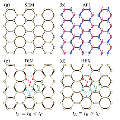
Figure 17: The graphene structures studied in Ref. 166. (a) SEM honeycomb, semimetallic; (b) AFI honeycomb antiferromagnetic insulator; (c) DIM dimerized Kekulé-like insulator; (d) HEX distorted hexagonal insulator. There are two carbons per unit cell in (a) and (b), six in (c) and (d). $t_{A}$, $t_{B}$, and $t_{C}$ schematically denote different hopping integrals magnitudes. Reprinted with permission from Sorella et al. (2018), Phys. Rev. Lett., published by APS in 2018.

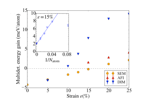
Figure 18: Energy gains by the resonance effect, measured by the energy per atom difference between the single determinant ansatz (Jastrow-Slater determinant WF) and the corresponding multideterminant JAGP WF. The largest energy gain occurs in the DIM state, underlining its resonating valence-bond nature, actually increasing for large strain $\varepsilon$. Small negative values at small strain are finite-size effects. Inset: finite-size scaling of this correlation energy gain in the DIM state at $\varepsilon$ = 15%. Reprinted with permission from Sorella et al. (2018), Phys. Rev. Lett., published by APS in 2018.

XII.5 Organic compounds: diradicals and conjugated systems

Diradical and conjugated organic compounds are other interesting applications of the RVB WF, because both static and dynamic correlation effects play important roles in these systems. A. Zen et al. found that the RVB WF gives a correct torsion barrier of the ethylene (C₂H₄) and the triple-singlet gap in the methylene (CH₂) Zen et al. (2014a). They also investigated the charge-transfer and diradical nature of the electronic states of the retinal minimal model (penta-2,4-dieniminium cation) at the VMC and LRDMC levels  Zen et al. (2015a). They proved that the dynamical electronic correlation is key to get a reliable ground state energy surface in proximity of the conical intersection between the electronic ground- and first excited-state of the molecule. Their obtained energy landscapes significantly different from the CASSCF ones, inverting the relative stability of several torsional paths, and similar to what was obtained by other correlated approaches. M. Barborini et al. applied VMC and LRDMC to calculate the torsion barriers of 1,3-butadiene and the ring-opening barrier of cyclobutene Barborini and Guidoni (2012), which are in good agreement with the experimental results. M. Barborini and E. Coccia investigated the potential energy curves of the two spin states of tetramethyleneethane (TME) molecule and the two anionic states of TME as a function of the torsion of the central dihedral angle Barborini and Coccia (2015). Through ab initio geometrical optimizations at the VMC level, they proposed possible structural interconversions between the states, which are in agreement with the ion photoelectron spectroscopy experiments.

The bond length alternation (BLA), namely, the impact on the geometry of the difference between the single and double carbon bonds, is one of the key structural descriptors in conjugated organic compounds. M. Barborini et al. investigated the effects of the static and dynamical electronic correlations on the BLA of the 1,3-butadiene Barborini and Guidoni (2015a) using a VMC-JAGP ansatz and other quantum chemistry calculations. They found inconsistency between BLAs obtained by CCSD(T)-CBS (the most accurate) and VMC-JAGP calculations, but the reason for the discrepancy is still unclear. They also investigated the structural properties of polyacetylene chains H-(C₂H₂)_n-H up to $N$ = 12 acetylene units Barborini and Guidoni (2015b), in which they revealed that the BLA obtained by the extrapolation to $n$ $\to$ $\infty$ is 0.0910(7) Å, which is compatible with the experimental data. E. Coccia et al. applied VMC to study geometries of the retinal model, the chromophore of the rhodopsin involved in the mechanism of vision, and discussed the effects of the electronic correlation on the BLA Coccia and Guidoni (2012); Coccia et al. (2013) by comparing with DFT and quantum chemistry methods. Wave-function and geometry optimizations of the retinal model were also performed in the presence of the protein field, classically described via electrostatic and mechanical interactions: the complex environment dramatically affects the BLA of the chromophore, which consistently increases with respect to the gas-phase case. They also performed VMC geometry optimization of the peridinin chromophore in order to verify the interplay between the BLA and the optical properties of a large conjugated moiety, involved in the light-harvesting step of photosynthesis in the peridinin-chlorophyll-protein complex Coccia et al. (2014). Comparison with DFT and wave-function approaches shows that the combined application of RVB-based VMC and Bethe-Salpeter methods for geometry and excitations, respectively, gives an accurate estimation of the electronic transition energies of peridinin. They recently applied VMC optimization to obtain a ground state structure of keto-1, enol-1, and enol-2 forms of oxyluciferin Coccia et al. (2017), which is used to calculate the $S^{1}$ $\leftarrow$ $S^{0}$ absorption energy based on the Bethe-Salpeter formalism. E. Coccia et al. carried out a systematic basis-set analysis on polarizability, quadrupole moment and electronic density of C₂H₂ molecule, with the aim to test VMC and LRDMC calculations in the presence of an external electric field Coccia et al. (2012). In particular, a relatively small hybrid (Gaussian + Slater functions) basis set was seen to be able to properly reproduce reference values.

XII.6 Metal-organic complexes

Recently, TurboRVB  has also been used to study metal-organic complexes. S. Chu et al. studied free-energy reaction barriers of water splitting reactions, using a simplified computational model based on the cobalt ion Chu et al. (2016) (Fig. 19). They found that the total free-energy differences of the water oxidation, computed at the QMC level, fairly agree with the experimental reference values, in a surprisingly better way than the corresponding CCSD(T) ones. M. Barborini and L. Guidoni applied VMC to tackle the geometry optimization of a Fe₂S₂(SH)₂^- model complex (High-Spin and Broken Symmetry states) Barborini and Guidoni (2016) based on the extended broken-symmetry (EBS) approach. The number of applications is still limited in this category, but the recent development of sophisticated transition-metal pseudopotentials will make it more feasible in the near future.

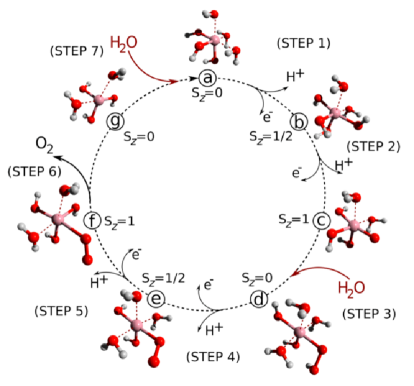
Figure 19: Reaction cycle involving the cobalt ion model, studied in Ref. 176 by VMC and LRDMC. The pink, red, and white balls represent the cobalt, oxygen, and hydrogen atoms, respectively. Reprinted with permission from Chu et al. (2016), J. Chem. Theory Comput., published by ACS in 2016.

XII.7 Crystals polymorphism

Ab initio electronic calculations allow one to study the phase stability between crystals polymorphs, by comparing the enthalpies or free energies, and by computing their equation of states (EOSs). As mentioned in the introduction, DFT’s predictive power strongly depends on the choice of the exchange and correlation functionals, sometimes causing qualitatively different phase stability predictions. On the other hand, VMC and LRDMC calculations do not suffer from this drawback in principle. S. Sorella et al. studied the pressure-induced metal-insulator transition in bulk silicon through EOS calculations  Sorella et al. (2011). They obtained a reasonable transition pressure at room temperature by VMC, however still a little far from the experimental value. N. Devaux et al. studied the $\alpha$-$\gamma$ phase transition in elemental cerium at the VMC and LRDMC levels Devaux et al. (2015). They revealed that the volume-collapse transition could be understood as a conventional first-order transition of electronic origin, induced by the $p$-$f$ hybridization, and by the strong local repulsion affecting the $f$ states. H. Hay et al. investigated the effect of long-range van der Waals forces in the SiO₂ polymorphs using DFT and QMC Hay et al. (2015). Their LRDMC calculations showed that the obtained energy differences in quartz-cristobalite and quartz-stishovite agree well with the experimental values within sub-chemical accuracy, implying that QMC is a promising method in describing both conventional and high-pressure SiO₂ polymorphs. Notice that, at present, only the zero-temperature energy (without the entropic term) is available at the VMC and LRDMC levels. Therefore, the entropic effects are estimated by DFT-PBE calculations Sorella et al. (2011). In the near future, it will be possible to estimate the entropic corrections directly within the VMC framework, via phonon calculations under the quasi-harmonic approximation. As described in Sec. IV, considering twist boundary conditions is essential to correct the one-body finite-size errors for periodic systems, especially in a metallic case. Although the twisted average approach is commonly used to correct the error, one can also use the exact special twist (EST) methodDagrada et al. (2016) developed by M. Dagrada et al. to save some computational cost. EST works even in realistic systems, namely, the bcc-hydrogen, the bcc-lithium, and the silicon in the high-pressure $\beta$-tin phaseDagrada et al. (2016).

XII.8 One-dimensional chains

One-dimensional chains of atoms have been intensively studied based on both effective and ab initio Hamiltonians, because they embody many important open questions in modern condensed matter physics, despite their simplicity. The finite or infinite hydrogen chains are ideal systems for this purpose, because it is not necessary to use a pseudopotential or to consider the relativistic effects. They are therefore benchmark systems. L. Stella et al. investigated the metal-insulator transition in the hydrogen chain by explicitly calculating the complex polarization Stella et al. (2011), as shown in Sec. XI. They found that the model has not a metal-insulator transition and always behaves as an insulating 1D Hubbard model at half-filling, at least for a large enough interatomic distance ($R>1$). M. Motta et al. (Simons Collaboration on the Many-Electron Problem) Motta et al. (2017) undertook a comprehensive benchmark study in the finite and infinite linear hydrogen chains using state-of-the-art many-body methods, including VMC and LRDMC with extrapolations to the thermodynamic and the complete-basis-set limits. They provide accurate potential energies curves online, which will be very useful for benchmarking other methods. They have recently investigated the ground states of the hydrogen-chain more in details, namely, the insulator-to-metal transition, dimerization, and magnetic phases Motta et al. (2019). They revealed a fascinating phase diagram, with several emergent quantum phases, depending on the interproton distance.

XII.9 Liquid and solid hydrogen/helium

Hydrogen behavior at high pressures is still not fully understood and subject of intense research. In 1935, Wigner and Huntington predicted its metallization upon compression Wigner and Huntington (1935), while Ashcroft also proposed its high-$T_{\text{c}}$ superconductivity Ashcroft (1968). Besides its fundamental interest as the simplest realistic condensed matter system in Nature, calculating its equilibrium properties remains of fundamental importance for planetary science applications Guillot (2005). This system is particularly challenging for DFT-based simulations, due to the presence of strong correlation effects and a subtle interplay between structural and electronic phase transitions. A straightforward way to study a phase diagram under pressure and at finite temperature in QMC is to apply the Langevin molecular dynamics described in Sec. VIII. First-order phase transitions can be identified from a discontinuous behavior in the calculated equation of state, and of pair correlation functions. C. Attaccalite and S. Sorella have formulated a second-order LD suitable for QMC simulation for the first time, as described in Sec. VIII. They applied it to assess the relative stability of solid and liquid hydrogen at high pressure and room temperature Attaccalite and Sorella (2008). Years later, in a series of works, G. Mazzola et al. applied this technique to study the proposed liquid-liquid transition (LLT) from a molecular insulating to an atomic conducting phase of hydrogen Mazzola et al. (2014); Mazzola and Sorella (2015). G. Mazzola and S. Sorella have also formulated the accelerated first-order LD Mazzola and Sorella (2017), as described in Sec. VIII, to study such an elusive phase transition with properly equilibrated simulations Mazzola and Sorella (2017). Finally, under the same framework the first QMC molecular dynamics simulations of an hydrogen-helium mixture has been performed at Jupiter’s interior conditions Mazzola et al. (2018). The study revealed that mixing He has a significant influence on the H metallization pressure as shown in Fig. 20, and provided useful benchmark for the equation of states currently adopted by the planetary science community. M. Dagrada et al. revealed that their developed EST technique also works well in the LD simulation for liquid hydrogen, but a perfect agreement with the twisted-average technique is achieved only when relatively large supercells are used Dagrada et al. (2016). Therefore, a careful finite size scaling analysis is needed when the EST technique is employed, though the thermodynamic limit extrapolation is much smoother at the special twist, saving some computational cost. Moreover, EST allows for the determinant/AGP optimization.

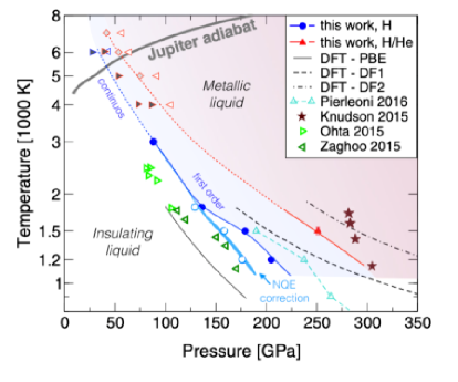
Figure 20: Phase Diagram of dense hydrogen and a hydrogen-helium mixture. “This work” refers to the results obtained by VMC-Langevin dynamics simulations. The shaded areas represent the liquid-liquid transitions (LLT) between the insulating-molecular and the metallic-atomic fluids. The solid symbols refer to their QMC LLTs for the pure hydrogen (blue circles) and for the hydrogen-helium mixture (red triangle), and the solid blue and red lines indicate first order LLTs. The empty (solid) left (right) triangles correspond to simulations displaying a clear atomic (molecular) behavior, on the other hand, the red diamonds represent an intermediate behavior. A calculated Jupiter’s adiabat calculated is shown as a gray line. Pure hydrogen first-order LLT predicted by QMC (cyan) and DFT (solid and dashed lines) are also shown. The light green and dark green triangles and the brown stars represent experimental results. Reprinted with permission from Mazzola et al. (2018), Phys. Rev. Lett., published by APS in 2018.

XII.10 Excited states

TurboRVB  allows studying not only the ground-state electronic properties but also excited states. It is trivial to obtain excitation properties when they are characterized by different particles or different spin projection, because these quantities are clearly conserved. For example, M. Barborini et al. calculated the ${}^{3}B_{1u}$ $\leftarrow$ ${}^{1}A_{g}$ vertical triplet excitation of the ethylene molecule and its adiabatic excitation ${}^{3}A_{1}$ $\leftarrow$ ${}^{1}A_{g}$Barborini et al. (2012). One can also deal with nontrivial cases based on a flexible symmetry-adapted RVB WF within its MO representation, which was proposed by N. Dupuy et al. in 2015 Dupuy et al. (2015). Instead of dealing with a linear combination of symmetry-adapted configuration state functions, they construct a symmetry-adapted RVB WF that accurately describes the targeted symmetry. They reported that their developed constrained (fixed-rank) minimization of the geminal expansion is stable without symmetry contamination of the starting excited state symmetry; as a result, the vertical ionization energies and the electron affinities of anthracene obtained by VMC and LRDMC calculations agree with the experimental values.

XII.11 Connection to experimental spectroscopies

M. Barborini et al. proposed a new ab initio approach to calculate quasiparticle WFs (QPWF) of isolated systems and resolved in momentum space, based on the correlated sampling technique. They applied the new approach to simulate Scanning Tunneling Microscopy (STM) images Barborini et al. (2016) and Angle-Resolved Photoemission Spectroscopy (ARPES) Barborini et al. (2018). The STM image of [CuCl₄]^2- obtained by this approach is shown in Fig. 21. It reveals that the electronic correlation has a significant effect on the QPWF in this system. Indeed, the resulting STM image clearly differs from that obtained by uncorrelated methods (i.e., the Hartree-Fock counterpart). In general, the electronic calculation should be useful to interpret the experimental results theoretically. We believe therefore that TurboRVB can become useful also for state-of-the-art research in this field.

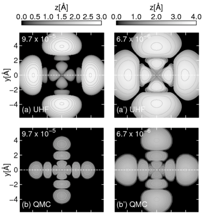
Figure 21: The STM images of in-plane [CuCl₄]^2- simulated using UHF and QMC calculations. The left column shows the isosurfaces of the square modulus of the eQPWF for a fixed value of probability density of 9.7 $\times$ 10^-5 Å^-3, while in the right column the isosurfaces take the value of 6.7 $\times$ 10^-6 Å^-3. The top panels ($a$ and $a^{\prime}$) display the LUMO+1 UHF molecular orbitals, while the middle panels ($b$ and $b^{\prime}$) display the QMC images. Reprinted with permission from Barborini et al. (2016), J. Chem. Theory Comput., published by ACS in 2016.

XIII Python module:Turbo-Genius

In general, a computational study involves many complicated operations, such as preparing input files, searching for optimal parameters, performing benchmark studies, transferring information coming from previous calculations to a subsequent simulation’s input file, and analyzing output files. Automatizing these operations can significantly save researcher’s burden, avoid trivial human errors, and is beneficial for accelerating the distribution of a computational package to a much wider community. We are now developing a python-based workflow system suitable for TurboRVB  named Turbo-Genius, like NexusKrogel (2016) and QMC-SWKonkov and Peverati (2019). The workflow system has been implemented in Python 3 in an object-oriented fashion, so the modules are highly extensible. Notice that, since TurboRVB  is an all-in-one package, any other commercial code is not necessary to run the code. There are two main modules, turbo-genius-serial.py and turbo-genius-sequential.py, which manage other modules/classes. The former allows one to perform a single job specified by an option (e.g., turbo-genius-serial.py -j makefort10), and the latter does a sequential job (e.g., makefort10.x $\to$ convertfort10mol.x $\to$ prep.x $\to$ turborvb.x). By using Turbo-Genius, one can also analyze a simulation output. For example, one can plot an optimization history, average the variational parameters after optimization, and search for an optimal number of equilibration steps and a reblocking length.Flyvbjerg and Petersen (1989) Turbo-Genius  is still at an early stage of development. However, its main features are already there. In the near future, the Turbo-Genius modules will be capable of sophisticated TurboRVB  jobs automatizations, as well as setting optimal parameters depending on target systems.

XIV Conclusions

In this paper, we have reviewed TurboRVB, an ab initio quantum Monte Carlo package featuring two well established QMC algorithms for electronic structure: variational Monte Carlo, and diffusion Monte Carlo. The beginning of the TurboRVB development dates back to 2003, with the Ph.D thesis project of M. Casula supervised by S. Sorella. Since then, TurboRVB has rapidly grown up, and it has been applied to the study of several molecular and condensed matter systems, from benzene to high-temperature superconducting materials. Central to this package are variational parameterizations of correlated electronic WFs in the product form $\Psi=\Phi_{\text{AS}}*\exp J$, made of an antisymmetric part ($\Phi_{\text{AS}}$), and a Jastrow factor ($J$).

Concerning the antisymmetric part, TurboRVB implements five ansätze (in order of decreasing variational flexibility): $\rm(\hskip 1.79993pti\hskip 1.79993pt)$ the Pfaffian (Pf), $\rm(\hskip 0.80002ptii\hskip 0.80002pt)$ the Pfaffian with constrained number of molecular orbitals (Pfn), $\rm(iii)$ the Antisymmetrized Geminal Power (AGP), $\rm(iv)$ the Antisymmetrized Geminal Power with constrained number of molecular orbitals (AGPn), and $\rm(\hskip 0.59998ptv\hskip 0.59998pt)$ the single Slater determinant (SD). Notably, the user can freely navigate between these ansätze. Indeed, the package includes conversion modules, which allow the user to choose the most suitable WF form for the target system.

All the above ansätze can be optimized by state-of-the-art algorithms, namely, the stochastic reconfiguration and the linear method, thus achieving highly accurate variational and fixed-node energies, with a computational cost remaining at the single-determinant level, thanks to efficient algorithmic developments.

The stochastic optimization of many variational parameters (so far up to the order of $10^{5}$) is feasible in TurboRVB thanks to an efficient evaluation of energy derivatives using the AAD. This algorithmic scheme, which gives the code an original architecture, drastically decreases the computational cost of ionic forces calculations, keeping them of order $N^{3}$. Thus, it paves the way for efficient structural optimizations and molecular dynamics simulations at the VMC level of theory. Indeed, by means of the TurboRVB  package, it is at present possible to perform QMC molecular dynamics simulations of dense hydrogen (with up to 256 ions) and liquid water (with up to 64 water molecules), with a remarkably large number of atoms, not far from the DFT state of the art. Thanks to TurboRVB, nuclear quantum effects are also accessible in a correlated electronic environment provided by the VMC WF.

Large scale calculations are possible with TurboRVB not only because of cutting-edge algorithmic developments but also by virtue of an efficient parallelization based on a hybrid MPI and OpenMP protocol, that is ideal for employing GPU accelerators as well, recently available in the most advanced HPC infrastructures.

A python wrapper, named Turbo-Genius, has recently been developed to make the code user-friendly, and to allow both beginners and professional users to handle it more efficiently. We will continue developing TurboRVB and Turbo-Genius to implement new QMC algorithms and to extend their range of applications for the current developers and expected new upcoming contributors and users.

XV Data availability

The data that supports the findings of this study are available within this article and the cited references. TurboRVB  is available from S.S.’s web site [https://people.sissa.it/$\sim$sorella/] upon request.

XVI Acknowledgements

The authors acknowledge all contributors for the development of the code TurboRVB over the last twenty years. We would especially like to acknowledge very fruitful collaborations with F. Becca, G. Carleo, C. Cavazzoni, N. Devaux, N. Dupuy, L. Guidoni, H. Hay, R. Hlubina, Y. Iqbal, R. Maezono, F. Mouhat, A. Parola, K. Seki, T. Shirakawa, L. Spanu, L. Stella, L.F. Tocchio, and S. Yunoki.

K.N. is grateful for computational resources from PRACE project No. 2019204934 and those from the facilities of Research Center for Advanced Computing Infrastructure at Japan Advanced Institute of Science and Technology (JAIST). K.N. also acknowledges a financial support from the Simons Foundation and that from Grant-in-Aid for Scientific Research on Innovative Areas (No. 16H06439). C.A. acknowledges funding from the European Union Seventh Framework Program under grant agreement No. 785219 Graphene Core 2 and COST Action TUMIEE CA17126. M.C. is grateful to the French grand équipement national de calcul intensif (GENCI) for the computational time provided through these years under the project number 0906493, for the funded PRACE projects Nos. 2012061116, 2015133179, 2016163936, and for the access to the Hokusai and K-computer granted by the Institute of Physical and Chemical Research (RIKEN). Y.L. was supported by the Argonne Leadership Computing Facility, which is a U.S. Department of Energy Office of Science User Facility operated under contract DE-AC02-06CH11357. A.Z.’s work is sponsored by the Air Force Office of Scientific Research, Air Force Material Command, U.S. Air Force, under Grant No. FA9550-19-1-7007. S.S. acknowledges a financial support from PRIN 2017BZPKSZ and computational resources from PRACE project No. 2019204934. S.S is also grateful for his wife L. Urgias for bearing the too many weekends spent for the development of TurboRVB.

We dedicate this paper to the memory of P.W. Anderson, remembering him as one of the most influential contributors to physics and chemistry of the past century, and in particular for deeply inspiring this work with his RVB theory of matter.

XVII References

References

- Ramprasad et al. (2017) R. Ramprasad, R. Batra, G. Pilania, A. Mannodi-Kanakkithodi, and C. Kim, Npj Comput. Mater. 3, 54 (2017).
- Rajan (2005) K. Rajan, Mater. Today 8, 38 (2005).
- Kohn and Sham (1965) W. Kohn and L. J. Sham, Phys. Rev. 140, A1133 (1965).
- Martin (2004) R. M. Martin, Electronic structure : basic theory and practical methods (Cambridge University Press, 2004).
- Medvedev et al. (2017) M. G. Medvedev, I. S. Bushmarinov, J. Sun, J. P. Perdew, and K. A. Lyssenko, Science 355, 49 (2017).
- Perdew and Schmidt (2001) J. P. Perdew and K. Schmidt, in AIP Conference Proceedings, Vol. 577 (AIP, 2001) pp. 1–20.
- Burke (2012) K. Burke, J. Chem. Phys. 136, 150901 (2012).
- Cohen et al. (2012) A. J. Cohen, P. Mori-Sánchez, and W. Yang, Chem. Rev. 112, 289 (2012).
- Szabo and Ostlund (1982) A. Szabo and N. Ostlund, Modern quantum chemistry (Macmillan PubliShing Co., Inc., 1982).
- Møller and Plesset (1934) C. Møller and M. S. Plesset, Phys. Rev. 46, 618 (1934).
- Knowles and Handy (1984) P. J. Knowles and N. C. Handy, Chem. Phys. Lett. 111, 315 (1984).
- Roos et al. (1980) B. O. Roos, P. R. Taylor, P. E. Si, et al., Chem. Phys. 48, 157 (1980).
- Čížek (1966) J. Čížek, J. Chem. Phys. 45, 4256 (1966).
- Foulkes et al. (2001) W. Foulkes, L. Mitas, R. Needs, and G. Rajagopal, Rev. Mod. Phys. 73, 33 (2001).
- Becca and Sorella (2017) F. Becca and S. Sorella, Quantum Monte Carlo approaches for correlated systems (Cambridge University Press, 2017).
- Metropolis and Ulam (1949) N. Metropolis and S. Ulam, J. Am. Stat. Assoc. 44, 335 (1949).
- Kim et al. (2018) J. Kim, A. D. Baczewski, T. D. Beaudet, A. Benali, M. C. Bennett, M. A. Berrill, N. S. Blunt, E. J. L. Borda, M. Casula, D. M. Ceperley, S. Chiesa, B. K. Clark, R. C. Clay, K. T. Delaney, M. Dewing, K. P. Esler, H. Hao, O. Heinonen, P. R. C. Kent, J. T. Krogel, I. Kylänpää, Y. W. Li, M. G. Lopez, Y. Luo, F. D. Malone, R. M. Martin, A. Mathuriya, J. McMinis, C. A. Melton, L. Mitas, M. A. Morales, E. Neuscamman, W. D. Parker, S. D. P. Flores, N. A. Romero, B. M. Rubenstein, J. A. R. Shea, H. Shin, L. Shulenburger, A. F. Tillack, J. P. Townsend, N. M. Tubman, B. V. D. Goetz, J. E. Vincent, D. C. Yang, Y. Yang, S. Zhang, and L. Zhao, J. Phys. Condens. Matter 30, 195901 (2018).
- Needs et al. (2009) R. J. Needs, M. D. Towler, N. D. Drummond, and P. L. Ríos, J. Phys. Condens. Matter 22, 023201 (2009).
- Wagner et al. (2009) L. K. Wagner, M. Bajdich, and L. Mitas, J. Comput. Phys. 228, 3390 (2009).
- (20) C. J. Umrigar and C. Filippi, “Cornell-Holland Ab-initio Materials Package (CHAMP),” http://pages.physics.cornell.edu/~cyrus/champ.html, [Online; accessed 27-Oct.-2019].
- Spencer et al. (2019) J. S. Spencer, N. S. Blunt, S. Choi, J. Etrych, M.-A. Filip, W. M. C. Foulkes, R. S. Franklin, W. J. Handley, F. D. Malone, V. A. Neufeld, et al., J. Chem. Theory Comput. 15, 1728 (2019).
- Zhang et al. (1997) S. Zhang, J. Carlson, and J. E. Gubernatis, Phys. Rev. B 55, 7464 (1997).
- Motta and Zhang (2018) M. Motta and S. Zhang, Wiley Interdiscip. Rev.: Comput. Mol. Sci. 8, e1364 (2018).
- Booth et al. (2009) G. H. Booth, A. J. Thom, and A. Alavi, J. Chem. Phys. 131, 054106 (2009).
- Booth et al. (2013) G. H. Booth, A. Grüneis, G. Kresse, and A. Alavi, Nature 493, 365 (2013).
- Thom (2010) A. J. W. Thom, Phys. Rev. Lett. 105, 263004 (2010).
- Spencer and Thom (2016) J. S. Spencer and A. J. Thom, J. Chem. Phys. 144, 084108 (2016).
- Blunt et al. (2014) N. S. Blunt, T. W. Rogers, J. S. Spencer, and W. M. C. Foulkes, Phys. Rev. B 89, 245124 (2014).
- Malone et al. (2015) F. D. Malone, N. Blunt, J. J. Shepherd, D. Lee, J. Spencer, and W. Foulkes, J. Chem. Phys. 143, 044116 (2015).
- Ten-no (2013) S. Ten-no, J. Chem. Phys. 138, 164126 (2013).
- Ohtsuka and Ten-no (2015) Y. Ohtsuka and S. Ten-no, J. Chem. Phys. 143, 214107 (2015).
- Ten-no (2017) S. Ten-no, J. Chem. Phys. 147, 244107 (2017).
- McClean and Aspuru-Guzik (2015) J. R. McClean and A. Aspuru-Guzik, Phys. Rev. A 91, 012311 (2015).
- Nagy and Savona (2018) A. Nagy and V. Savona, Phys. Rev. A 97, 052129 (2018).
- Pauling (1960) L. Pauling, The Nature of the Chemical Bond (Cornell university press, 1960).
- Anderson (1973) P. Anderson, Mater. Res. Bull. 8, 153 (1973).
- Nakano et al. (2020) K. Nakano, R. Maezono, and S. Sorella, Phys. Rev. B 101, 155106 (2020).
- Umrigar (1993) C. Umrigar, Phys. Rev. Lett. 71, 408 (1993).
- Stedman et al. (1998) M. Stedman, W. Foulkes, and M. Nekovee, J. Chem. Phys. 109, 2630 (1998).
- Flyvbjerg and Petersen (1989) H. Flyvbjerg and H. G. Petersen, J. Chem. Phys. 91, 461 (1989).
- Sorella and Capriotti (2010) S. Sorella and L. Capriotti, J. Chem. Phys. 133, 234111 (2010).
- Sorella (1998) S. Sorella, Phys. Rev. Lett. 80, 4558 (1998).
- Sorella et al. (2007) S. Sorella, M. Casula, and D. Rocca, J. Chem. Phys. 127, 014105 (2007).
- Sorella (2005) S. Sorella, Phys. Rev. B 71, 241103 (2005).
- Umrigar et al. (2007) C. J. Umrigar, J. Toulouse, C. Filippi, S. Sorella, and R. G. Hennig, Phys. Rev. Lett. 98, 110201 (2007).
- Toulouse and Umrigar (2007) J. Toulouse and C. J. Umrigar, J. Chem. Phys. 126, 084102 (2007).
- Casula et al. (2005a) M. Casula, C. Filippi, and S. Sorella, Phys. Rev. Lett. 95, 100201 (2005a).
- Ten Haaf et al. (1995) D. F. Ten Haaf, H. J. Van Bemmel, J. M. Van Leeuwen, W. Van Saarloos, and D. M. Ceperley, Phys. Rev. B 51, 13039 (1995).
- Calandra Buonaura and Sorella (1998) M. Calandra Buonaura and S. Sorella, Phys. Rev. B 57, 11446 (1998).
- Sorella and Capriotti (2000) S. Sorella and L. Capriotti, Phys. Rev. B 61, 2599 (2000).
- Casula (2005) M. Casula, New QMC approaches for the simulation of electronic systems: a first application to aromatic molecules and transition metal compounds, Ph.D. thesis, International School for Advanced Studies (SISSA) (2005).
- Casula et al. (2010) M. Casula, S. Moroni, S. Sorella, and C. Filippi, J. Chem. Phys. 132, 154113 (2010).
- Casula (2006) M. Casula, Phys. Rev. B 74, 161102 (2006).
- Zen et al. (2019) A. Zen, J. G. Brandenburg, A. Michaelides, and D. Alfè, J. Chem. Phys. 151, 134105 (2019).
- Note (1) The correlation energy is typically defined as the difference between the exact energy and the Hartree-Fock energy, which is the variational minimum for a SD ansatz.
- Note (2) However, the Jastrow factor makes not factorizable when expectation values of quantum operators are evaluated. For this reason it is not a feasible route to traditional quantum chemistry approaches, as it requires stochastic approaches to evaluate efficiently the corresponding multidimensional integrals.
- López Ríos et al. (2006) P. López Ríos, A. Ma, N. D. Drummond, M. D. Towler, and R. J. Needs, Phys. Rev. E 74, 066701 (2006).
- Note (3) Indeed, with backflow each time an electron is moved, all the entries in (or several of them, if cut-offs are used) can be changed, resulting in a much more expensive algorithm.
- Kato (1957) T. Kato, Commun. Pure Appl. Math. 10, 151 (1957).
- Bajdich et al. (2006) M. Bajdich, L. Mitas, G. Drobný, L. K. Wagner, and K. E. Schmidt, Phys. Rev. Lett. 96, 130201 (2006).
- Bajdich et al. (2008) M. Bajdich, L. Mitas, L. K. Wagner, and K. E. Schmidt, Phys. Rev. B 77, 115112 (2008).
- Genovese et al. (2019a) C. Genovese, T. Shirakawa, and S. Sorella, arXiv , 1911.09748 (2019a).
- Kasteleyn (1963) P. Kasteleyn, J. Math. Phys. 4, 287 (1963).
- Note (4) Some properties of the Pfaffian operator and their proofs are given in Bajdich et al. (2008).
- Casula and Sorella (2003) M. Casula and S. Sorella, J. Chem. Phys. 119, 6500 (2003).
- Zen et al. (2014a) A. Zen, E. Coccia, Y. Luo, S. Sorella, and L. Guidoni, J. Chem. Theory Comput. 10, 1048 (2014a).
- Zen et al. (2015a) A. Zen, E. Coccia, S. Gozem, M. Olivucci, and L. Guidoni, J. Chem. Theory Comput. 11, 992 (2015a).
- Note (5) can be computed after a standard block diagonalization of the matrix , being an unitary matrix and is a diagonal matrix, such that , where is the diagonal matrix obtained by taking the inverse square root of each diagonal element of . At this stage we carefully remove from the basis the elements corresponding to the smallest eigenvalues in order to work with a sufficiently large condition number that guarantees stable finite precision numerical calculations.
- Genovese et al. (2020) C. Genovese, T. Shirakawa, K. Nakano, and S. Sorella, arXiv , 2002.03347 (2020).
- Note (6) The nonzero eigenvalues of are .
- Marchi et al. (2009) M. Marchi, S. Azadi, M. Casula, and S. Sorella, J. Chem. Phys. 131, 154116 (2009).
- Note (7) The output of AAD are matrices where is either the log of the WF or the corresponding local energy computed on a given configuration. Then the projected derivatives corresponding to easily follows from Eq. 67, by applying the chain rule.
- Note (8) It shall be noticed that there is not necessarily one leading term in the expansion in Eq. 71. For instance, when the term with have equal weight to the term .
- Note (9) The seniority number is the number of unpaired electrons in a determinant.
- Pritchard et al. (2019) B. P. Pritchard, D. Altarawy, B. T. Didier, T. D. Gibson, and T. L. Windus, J. Chem. Inf. Model. 59, 4814 (2019).
- Trail and Needs (2015) J. R. Trail and R. J. Needs, J. Chem. Phys. 142, 064110 (2015).
- Krogel et al. (2016) J. T. Krogel, J. A. Santana, and F. A. Reboredo, Phys. Rev. B 93, 75143 (2016).
- Trail and Needs (2017) J. R. Trail and R. J. Needs, J. Chem. Phys. 146, 204107 (2017).
- Bennett et al. (2017) M. C. Bennett, C. A. Melton, A. Annaberdiyev, G. Wang, L. Shulenburger, and L. Mitas, J. Chem. Phys. 147, 224106 (2017).
- Bennett et al. (2018) M. C. Bennett, G. Wang, A. Annaberdiyev, C. A. Melton, L. Shulenburger, and L. Mitas, J. Chem. Phys. 149, 104108 (2018).
- Annaberdiyev et al. (2018) A. Annaberdiyev, G. Wang, C. A. Melton, M. Chandler Bennett, L. Shulenburger, and L. Mitas, J. Chem. Phys. 149, 134108 (2018).
- Burkatzki et al. (2007) M. Burkatzki, C. Filippi, and M. Dolg, J. Chem. Phys. 126, 234105 (2007).
- Burkatzki et al. (2008) M. Burkatzki, C. Filippi, and M. Dolg, J. Chem. Phys. 129, 164115 (2008).
- Fahy et al. (1990) S. Fahy, X. W. Wang, and S. G. Louie, Phys. Rev. B 42, 3503 (1990).
- Sorella et al. (2015) S. Sorella, N. Devaux, M. Dagrada, G. Mazzola, and M. Casula, J. Chem. Phys. 143, 244112 (2015).
- Lin et al. (2001) C. Lin, F. H. Zong, and D. M. Ceperley, Phys. Rev. E 64, 016702 (2001).
- Dagrada et al. (2016) M. Dagrada, S. Karakuzu, V. L. Vildosola, M. Casula, and S. Sorella, Phys. Rev. B 94, 245108 (2016).
- Rajagopal et al. (1994) G. Rajagopal, R. J. Needs, S. Kenny, W. M. C. Foulkes, and A. James, Phys. Rev. Lett. 73, 1959 (1994).
- Rajagopal et al. (1995) G. Rajagopal, R. Needs, A. James, S. Kenny, and W. Foulkes, Phys. Rev. B 51, 10591 (1995).
- Pisani et al. (1988) C. Pisani, R. Dovesi, and C. Roetti, in Hartree-Fock ab initio treatment of crystalline systems, Vol. 48 (Springer Berlin, 1988).
- Dovesi et al. (2018) R. Dovesi, A. Erba, R. Orlando, C. M. Zicovich-Wilson, B. Civalleri, L. Maschio, M. Rérat, S. Casassa, J. Baima, S. Salustro, et al., Wiley Interdiscip. Rev.: Comput. Mol. Sci. 8, e1360 (2018).
- Karakuzu et al. (2017) S. Karakuzu, L. F. Tocchio, S. Sorella, and F. Becca, Phys. Rev. B 96, 205145 (2017).
- Fraser et al. (1996) L. M. Fraser, W. M. C. Foulkes, G. Rajagopal, R. J. Needs, S. D. Kenny, and A. J. Williamson, Phys. Rev. B 53, 1814 (1996).
- Williamson et al. (1997) A. J. Williamson, G. Rajagopal, R. J. Needs, L. M. Fraser, W. M. C. Foulkes, Y. Wang, and M.-Y. Chou, Phys. Rev. B 55, R4851 (1997).
- Kent et al. (1999) P. R. C. Kent, R. Q. Hood, A. J. Williamson, R. J. Needs, W. M. C. Foulkes, and G. Rajagopal, Phys. Rev. B 59, 1917 (1999).
- Kwee et al. (2008) H. Kwee, S. Zhang, and H. Krakauer, Phys. Rev. Lett. 100, 126404 (2008).
- Chiesa et al. (2006) S. Chiesa, D. M. Ceperley, R. M. Martin, and M. Holzmann, Phys. Rev. Lett. 97, 076404 (2006).
- Frisch et al. (2016) M. J. Frisch, G. W. Trucks, H. B. Schlegel, G. E. Scuseria, M. A. Robb, J. R. Cheeseman, G. Scalmani, V. Barone, G. A. Petersson, H. Nakatsuji, X. Li, M. Caricato, A. V. Marenich, J. Bloino, B. G. Janesko, R. Gomperts, B. Mennucci, H. P. Hratchian, J. V. Ortiz, A. F. Izmaylov, J. L. Sonnenberg, D. Williams-Young, F. Ding, F. Lipparini, F. Egidi, J. Goings, B. Peng, A. Petrone, T. Henderson, D. Ranasinghe, V. G. Zakrzewski, J. Gao, N. Rega, G. Zheng, W. Liang, M. Hada, M. Ehara, K. Toyota, R. Fukuda, J. Hasegawa, M. Ishida, T. Nakajima, Y. Honda, O. Kitao, H. Nakai, T. Vreven, K. Throssell, J. A. Montgomery, Jr., J. E. Peralta, F. Ogliaro, M. J. Bearpark, J. J. Heyd, E. N. Brothers, K. N. Kudin, V. N. Staroverov, T. A. Keith, R. Kobayashi, J. Normand, K. Raghavachari, A. P. Rendell, J. C. Burant, S. S. Iyengar, J. Tomasi, M. Cossi, J. M. Millam, M. Klene, C. Adamo, R. Cammi, J. W. Ochterski, R. L. Martin, K. Morokuma, O. Farkas, J. B. Foresman, and D. J. Fox, “Gaussian 16 Revision C.01,” (2016), gaussian Inc. Wallingford CT.
- Giannozzi et al. (2009) P. Giannozzi, S. Baroni, N. Bonini, M. Calandra, R. Car, C. Cavazzoni, D. Ceresoli, G. L. Chiarotti, M. Cococcioni, I. Dabo, et al., J. Phys. Condens. Matter. 21, 395502 (2009).
- Perdew and Zunger (1981) J. P. Perdew and A. Zunger, Phys. Rev. B 23, 5048 (1981).
- Azadi et al. (2010) S. Azadi, C. Cavazzoni, and S. Sorella, Phys. Rev. B 82, 125112 (2010).
- Dunning Jr (1989) T. H. Dunning Jr, J. Chem. Phys. 90, 1007 (1989).
- Nakano et al. (2019) K. Nakano, R. Maezono, and S. Sorella, J. Chem. Theory Comput. 15, 4044 (2019).
- Assaraf et al. (2017) R. Assaraf, S. Moroni, and C. Filippi, J. Chem. Theory Comput. 13, 5273 (2017).
- Umrigar (2009) C. Umrigar, Int. J. Quantum Chem 36, 217 (2009).
- Attaccalite and Sorella (2008) C. Attaccalite and S. Sorella, Phys. Rev. Lett. 100, 114501 (2008).
- Zen et al. (2013) A. Zen, Y. Luo, S. Sorella, and L. Guidoni, J. Chem. Theory Comput. 9, 4332 (2013).
- Mazzola et al. (2012) G. Mazzola, A. Zen, and S. Sorella, J. Chem. Phys. 137, 134112 (2012).
- Amari (1998) S.-I. Amari, Neural Comput. 10, 251 (1998).
- Neuscamman et al. (2012) E. Neuscamman, C. J. Umrigar, and G. K.-L. Chan, Phys. Rev. B 85, 045103 (2012).
- Luo et al. (2014) Y. Luo, A. Zen, and S. Sorella, J. Chem. Phys. 141, 194112 (2014).
- Box and Muller (1958) G. E. P. Box and M. E. Muller, Ann. Math. Statist. 29, 610 (1958).
- Mazzola et al. (2014) G. Mazzola, S. Yunoki, and S. Sorella, Nat. Commun. 5, 3487 (2014).
- Mouhat et al. (2017) F. Mouhat, S. Sorella, R. Vuilleumier, A. M. Saitta, and M. Casula, J. Chem. Theory Comput. 13, 2400 (2017).
- Trotter (1959) H. F. Trotter, Proc. Amer. Math. Soc. 10, 545 (1959).
- Tuckerman et al. (1992) M. Tuckerman, B. J. Berne, and G. J. Martyna, J. Chem. Phys. 97, 1990 (1992).
- Sexton and Weingarten (1992) J. C. Sexton and D. H. Weingarten, Nucl. Phys. B 380, 667 (1992).
- Ceriotti et al. (2010) M. Ceriotti, M. Parrinello, T. E. Markland, and D. E. Manolopoulos, J. Chem. Phys. 133, 124104 (2010).
- Mazzola and Sorella (2017) G. Mazzola and S. Sorella, Phys. Rev. Lett. 118, 015703 (2017).
- Mazzola et al. (2018) G. Mazzola, R. Helled, and S. Sorella, Phys. Rev. Lett. 120, 025701 (2018).
- Note (10) We assume, without loss of generality, that .
- Assaraf et al. (2007) R. Assaraf, M. Caffarel, and A. Scemama, Phys. Rev. E 75, 035701 (2007).
- Stella et al. (2011) L. Stella, C. Attaccalite, S. Sorella, and A. Rubio, Phys. Rev. B 84, 245117 (2011).
- Genovese et al. (2019b) C. Genovese, A. Meninno, and S. Sorella, J. Chem. Phys. 150, 084102 (2019b).
- Resta and Sorella (1999) R. Resta and S. Sorella, Phys. Rev. Lett. 82, 370 (1999).
- Capello et al. (2005) M. Capello, F. Becca, M. Fabrizio, S. Sorella, and E. Tosatti, Phys. Rev. Lett. 94, 026406 (2005).
- Casula et al. (2004) M. Casula, C. Attaccalite, and S. Sorella, J. Chem. Phys. 121, 7110 (2004).
- Sorella and Zen (2014) S. Sorella and A. Zen, “The new resonating valence bond method for ab-initio electronic simulations,” in Many-Electron Approaches in Physics, Chemistry and Mathematics: A Multidisciplinary View, edited by V. Bach and L. Delle Site (Springer International Publishing, Cham, 2014) pp. 377–392.
- Zen et al. (2014b) A. Zen, B. L. Trout, and L. Guidoni, J. Chem. Phys. 141, 014305 (2014b).
- Casula et al. (2009) M. Casula, M. Marchi, S. Azadi, and S. Sorella, Chem. Phys. Lett. 477, 255 (2009).
- Casula et al. (2005b) M. Casula, S. Yunoki, C. Attaccalite, and S. Sorella, Comput. Phys. Commun. 169, 386 (2005b).
- Dupuy and Casula (2018) N. Dupuy and M. Casula, J. Chem. Phys. 148, 134112 (2018).
- Sterpone et al. (2008) F. Sterpone, L. Spanu, L. Ferraro, S. Sorella, and L. Guidoni, J. Chem. Theory Comput. 4, 1428 (2008).
- Zen et al. (2015b) A. Zen, Y. Luo, G. Mazzola, L. Guidoni, and S. Sorella, J. Chem. Phys. 142, 144111 (2015b).
- Dagrada et al. (2014) M. Dagrada, M. Casula, A. M. Saitta, S. Sorella, and F. Mauri, J. Chem. Theory Comput. 10, 1980 (2014).
- Note (11) A theory is size-consistent if the energy of the supersystem made of two fragments A and B at a sufficiently large distance is equal to the sum of the energy of the fragments. When a theory is size consistent it is equivalent to take as reference energy for a interaction energy evaluation the sum of the fragments or the supersystem with the fragments far apart, whereas if the theory is not there is an arbitrary shift as large as in the interaction energy.
- Note (12) JSD and JAGP could describe the O-O system if the number of unpaired is changed, for instance if four unpaired are used. However, this is not the right parametrization of the O2 molecule.
- Toulouse and Umrigar (2008) J. Toulouse and C. J. Umrigar, J. Chem. Phys. 128, 174101 (2008).
- Aziz and Slaman (1989) R. A. Aziz and M. Slaman, Chem. Phys. 130, 187 (1989).
- Merritt et al. (2009) J. M. Merritt, V. E. Bondybey, and M. C. Heaven, Science 324, 1548 (2009).
- Langhoff and Bauschlicher (1991) S. R. Langhoff and C. W. Bauschlicher, J. Chem. Phys. 95, 5882 (1991).
- Bytautas and Ruedenberg (2005) L. Bytautas and K. Ruedenberg, J. Chem. Phys. 122, 154110 (2005).
- Zen et al. (2012) A. Zen, D. Zhelyazov, and L. Guidoni, J. Chem. Theory Comput. 8, 4204 (2012).
- Note (13) Indeed, in order to improve the precision by an order of magnitude the sampling (so, the computational cost) has to be increased by two orders of magnitude. Considering that the evaluation of the energy and all the force components in TurboRVB costs only 4 times the evaluation of only the energy with the same sampling (see Sec. VI), the speedup is 100/4=25.
- Luo and Sorella (2015) Y. Luo and S. Sorella, Front. Mater. 2, 29 (2015).
- Grimme et al. (2010) S. Grimme, J. Antony, S. Ehrlich, and H. Krieg, J. Chem. Phys. 132, 154104 (2010).
- Goetz and Neuscamman (2017) B. V. D. Goetz and E. Neuscamman, J. Chem. Theory Comput. 13, 2035 (2017).
- Umrigar et al. (1993) C. Umrigar, M. Nightingale, and K. Runge, J. Chem. Phys. 99, 2865 (1993).
- Zen et al. (2016a) A. Zen, S. Sorella, M. J. Gillan, A. Michaelides, and D. Alfè, Phys. Rev. B 93, 241118 (2016a).
- Nemec et al. (2010) N. Nemec, M. D. Towler, and R. Needs, J. Chem. Phys. 132, 034111 (2010).
- Beaudet et al. (2008) T. D. Beaudet, M. Casula, J. Kim, S. Sorella, and R. M. Martin, J. Chem. Phys. 129, 164711 (2008).
- Spanu et al. (2009) L. Spanu, S. Sorella, and G. Galli, Phys. Rev. Lett. 103, 196401 (2009).
- Zen et al. (2016b) A. Zen, L. M. Roch, S. J. Cox, X. L. Hu, S. Sorella, D. Alfè, and A. Michaelides, J. Phys. Chem. C 120, 26402 (2016b).
- Nissenbaum et al. (2009) D. Nissenbaum, L. Spanu, C. Attaccalite, B. Barbiellini, and A. Bansil, Phys. Rev. B 79, 035416 (2009).
- Ferlat et al. (2019) G. Ferlat, M. Hellgren, F.-X. Coudert, H. Hay, F. Mauri, and M. Casula, Phys. Rev. Materials 3, 063603 (2019).
- Calandra et al. (1998) M. Calandra, F. Becca, and S. Sorella, Phys. Rev. Lett. 81, 5185 (1998).
- Capriotti et al. (1999) L. Capriotti, A. E. Trumper, and S. Sorella, Phys. Rev. Lett. 82, 3899 (1999).
- Becca et al. (2000) F. Becca, M. Capone, and S. Sorella, Phys. Rev. B 62, 12700 (2000).
- Capriotti et al. (2001) L. Capriotti, F. Becca, A. Parola, and S. Sorella, Phys. Rev. Lett. 87, 097201 (2001).
- Sorella et al. (2002) S. Sorella, G. B. Martins, F. Becca, C. Gazza, L. Capriotti, A. Parola, and E. Dagotto, Phys. Rev. Lett. 88, 117002 (2002).
- Bednorz and Müller (1986) J. G. Bednorz and K. A. Müller, Z. Phys. B 64, 189 (1986).
- Kamihara et al. (2008) Y. Kamihara, T. Watanabe, M. Hirano, and H. Hosono, J. Am. Chem. Soc. 130, 3296 (2008).
- Marchi et al. (2011) M. Marchi, S. Azadi, and S. Sorella, Phys. Rev. Lett. 107, 086807 (2011).
- Casula and Sorella (2013) M. Casula and S. Sorella, Phys. Rev. B 88, 155125 (2013).
- Busemeyer et al. (2016) B. Busemeyer, M. Dagrada, S. Sorella, M. Casula, and L. K. Wagner, Phys. Rev. B 94, 035108 (2016).
- Sorella et al. (2018) S. Sorella, K. Seki, O. O. Brovko, T. Shirakawa, S. Miyakoshi, S. Yunoki, and E. Tosatti, Phys. Rev. Lett. 121, 066402 (2018).
- Barborini and Guidoni (2012) M. Barborini and L. Guidoni, J. Chem. Phys. 137, 224309 (2012).
- Barborini and Coccia (2015) M. Barborini and E. Coccia, J. Chem. Theory Comput. 11, 5696 (2015).
- Barborini and Guidoni (2015a) M. Barborini and L. Guidoni, J. Chem. Theory Comput. 11, 508 (2015a).
- Barborini and Guidoni (2015b) M. Barborini and L. Guidoni, J. Chem. Theory Comput. 11, 4109 (2015b).
- Coccia and Guidoni (2012) E. Coccia and L. Guidoni, J. Comput. Chem. 33, 2332 (2012).
- Coccia et al. (2013) E. Coccia, D. Varsano, and L. Guidoni, J. Chem. Theory Comput. 9, 8 (2013).
- Coccia et al. (2014) E. Coccia, D. Varsano, and L. Guidoni, J. Chem. Theory Comput. 10, 501 (2014).
- Coccia et al. (2017) E. Coccia, D. Varsano, and L. Guidoni, J. Chem. Theory Comput. 13, 4357 (2017).
- Coccia et al. (2012) E. Coccia, O. Chernomor, M. Barborini, S. Sorella, and L. Guidoni, J. Chem. Theory Comput. 8, 1952 (2012).
- Chu et al. (2016) S. Chu, E. Coccia, M. Barborini, and L. Guidoni, J. Chem. Theory Comput. 12, 5803 (2016).
- Barborini and Guidoni (2016) M. Barborini and L. Guidoni, J. Chem. Phys. 145, 124107 (2016).
- Sorella et al. (2011) S. Sorella, M. Casula, L. Spanu, and A. Dal Corso, Phys. Rev. B 83, 075119 (2011).
- Devaux et al. (2015) N. Devaux, M. Casula, F. Decremps, and S. Sorella, Phys. Rev. B 91, 081101 (2015).
- Hay et al. (2015) H. Hay, G. Ferlat, M. Casula, A. P. Seitsonen, and F. Mauri, Phys. Rev. B 92, 144111 (2015).
- Motta et al. (2017) M. Motta, D. M. Ceperley, G. K.-L. Chan, J. A. Gomez, E. Gull, S. Guo, C. A. Jiménez-Hoyos, T. N. Lan, J. Li, F. Ma, A. J. Millis, N. V. Prokof’ev, U. Ray, G. E. Scuseria, S. Sorella, E. M. Stoudenmire, Q. Sun, I. S. Tupitsyn, S. R. White, D. Zgid, and S. Zhang (Simons Collaboration on the Many-Electron Problem), Phys. Rev. X 7, 031059 (2017).
- Motta et al. (2019) M. Motta, C. Genovese, F. Ma, Z.-H. Cui, R. Sawaya, G. K. Chan, N. Chepiga, P. Helms, C. Jimenez-Hoyos, A. J. Millis, et al., arXiv , 1911.01618 (2019).
- Wigner and Huntington (1935) E. Wigner and H. Huntington, J. Chem. Phys. 3, 764 (1935).
- Ashcroft (1968) N. W. Ashcroft, Phys. Rev. Lett. 21, 1748 (1968).
- Guillot (2005) T. Guillot, Annu. Rev. Earth Planet. Sci. 33, 493 (2005).
- Mazzola and Sorella (2015) G. Mazzola and S. Sorella, Phys. Rev. Lett. 114, 105701 (2015).
- Barborini et al. (2012) M. Barborini, S. Sorella, and L. Guidoni, J. Chem. Theory Comput. 8, 1260 (2012).
- Dupuy et al. (2015) N. Dupuy, S. Bouaouli, F. Mauri, S. Sorella, and M. Casula, J. Chem. Phys. 142, 214109 (2015).
- Barborini et al. (2016) M. Barborini, S. Sorella, M. Rontani, and S. Corni, J. Chem. Theory Comput. 12, 5339 (2016).
- Barborini et al. (2018) M. Barborini, S. Sorella, M. Rontani, and S. Corni, J. Chem. Phys. 149, 154102 (2018).
- Krogel (2016) J. T. Krogel, Comput. Phys. Commun. 198, 154 (2016).
- Konkov and Peverati (2019) V. Konkov and R. Peverati, SoftwareX 9, 7 (2019).