Distributed Non-Convex Optimization with Sublinear Speedup under Intermittent Client Availability

Abstract.

Federated learning is a new distributed machine learning framework, where a bunch of heterogeneous clients collaboratively train a model without sharing training data. In this work, we consider a practical and ubiquitous issue when deploying federated learning in mobile environments: intermittent client availability, where the set of eligible clients may change during the training process. Such intermittent client availability would seriously deteriorate the performance of the classical Federated Averaging algorithm (FedAvg for short). Thus, we propose a simple distributed non-convex optimization algorithm, called Federated Latest Averaging (FedLaAvg for short), which leverages the latest gradients of all clients, even when the clients are not available, to jointly update the global model in each iteration. Our theoretical analysis shows that FedLaAvg attains the convergence rate of $O(E^{1/2}/(N^{1/4}T^{1/2}))$, achieving a sublinear speedup with respect to the total number of clients. We implement FedLaAvg along with several baselines and evaluate them over the benchmarking MNIST and Sentiment140 datasets. The evaluation results demonstrate that FedLaAvg achieves more stable training than FedAvg in both convex and non-convex settings and indeed reaches a sublinear speedup.

1. Introduction

Federated Learning (FL) is a new paradigm of distributed machine learning (Li et al., 2019a; Kairouz et al., 2019; McMahan et al., 2017). It allows multiple clients to collaboratively train a global model without needing to upload local data to a centralized cloud server. In the FL setting, data are massively distributed over clients, with non-IID distribution (Hsieh et al., 2019; Li et al., 2020b) and unbalance in quantity (Mohri et al., 2019); in these ways, FL is distinguished from traditional distributed optimization (Li et al., 2014). Furthermore, the agents participating in FL are typically unreliable heterogeneous clients, e.g., mobile devices, with limited computation resources and unstable communication links (Tu et al., 2020; Hu et al., 2020; Wu et al., 2020; Li et al., 2019b; Wang et al., 2020), resulting in a varying set of eligible clients during the training process. These new features pose challenges in designing and analyzing learning algorithms for FL.

One of the leading challenges in deploying FL systems is client availability, where the clients may not be available throughout the entire training process. Consider the typical FL scenario where Google’s mobile keyboard Gboard polishes its language models among numerous mobile-device users (Bonawitz et al., 2019; Yang et al., 2018; Hard et al., 2018). To minimize the negative impact on user experience, only devices that meet certain requirements (e.g., charging, idle, and free Wi-Fi) are eligible for model training. These requirements are usually met at night local time but are not satisfied in the daytime when the devices are busy. Such intermittent client availability would introduce bias into training data. In particular, the clients with longer time available are more likely to be selected to participate, and thus their training data would be over-represented. In contrast, the training data of the clients, who have shorter time available and lower chance to be chosen, may be under-represented. Further, if the free resources on local devices (e.g., CPU and RAM) are also incorporated, the availability patterns of different clients would be more diverse, implying that the data representations are more differentiated in the collaborative training process. Nevertheless, the test data distribution, which is irrelevant with client availability in the training phase, would be inconsistent with the training data distribution. This inconsistency is also known as dataset shift (Quiñonero-Candela et al., 2009; Moreno-Torres et al., 2012), a notorious obstacle to the convergence of machine learning algorithms (Subbaswamy et al., 2019; Snoek et al., 2019), which also exists in FL, and can degrade the generalization ability of FL algorithms.

Existing work in the literature has not touched the issue of intermittent client availability, and the convergence analysis of FL algorithms always requires all the clients to be available throughout the training process. In this case, there is no bias in the training data, which is an essential condition to obtain the positive convergence results. Much effort (Wang and Joshi, 2018; Yu et al., 2019b; Khaled et al., 2019; Stich, 2019; Stich and Karimireddy, 2019; Li et al., 2020a; Karimireddy et al., 2020; Cho et al., 2020) has been expended in proving the convergence of the classical FedAvg algorithm (McMahan et al., 2017). One line of work (Wang and Joshi, 2018; Yu et al., 2019b; Khaled et al., 2019; Stich, 2019; Stich and Karimireddy, 2019) assumed that all the clients are available and participate in each iteration of the training, to establish the $O(1/\sqrt{NT})$ convergence of FedAvg. However, the requirement of full client participation would significantly increase the synchronization latency of the collaborative training process, and is hard to be satisfied in practical cross-device FL scenarios. Another line of work (Li et al., 2020a; Karimireddy et al., 2020; Cho et al., 2020) allowed partial client participation but required all the clients to be available, to proved an $O(1/T)$ convergence of FedAvg. In their analysis, clients are selected either uniformly at random (Li et al., 2020a; Karimireddy et al., 2020) or according to a certain strategy (Cho et al., 2020), which are, however, possible only if all clients are available.

In this work, we integrate the consideration of intermittent client availability into the design and analysis of the FL algorithm. We first formulate a practical model for intermittent client availability in FL; this model allows the set of available clients to follow any time-varying distribution, with the assumption that each client needs to be available at least once during any period with length $E$. Under such a client availability model, FedAvg would diverge even in a simple learning scenario with a quadratic objective (shown in Section 3.1), because the training data are biased towards those highly available clients. For general distributed non-convex optimization, we propose a simple Federated Latest Averaging algorithm, namely FedLaAvg, to approximately balance the influence of each client’s data on the global model training. Specifically, instead of averaging only the gradients collected from participating clients, FedLaAvg averages the latest gradients of all clients. By setting appropriate parameters, we can prove an $O(E^{1/2}/(N^{1/4}T^{1/2}))$ convergence for FedLaAvg, implying that FedLaAvg can achieve a sublinear speedup with respect to the total number of clients. We summarize our contributions as follows.

• To the best of our knowledge, we are the first to study the problem of intermittent client availability in FL, an ubiquitous phenomenon in practical mobile environments, and present a formal formulation thereof.

• We demonstrate that even with exact (not stochastic) gradient descent, two clients in the system, one local iteration on either client, and a simple quadratic (convex) optimization objective, FedAvg can diverge due to intermittent client availability.

• We identify the reasons behind the divergence of FedAvg and further propose a convergent algorithm FedLaAvg, which aggregates the latest gradients of all clients in each training iteration. Our theoretical analysis shows the $O(E^{1/2}/(N^{1/4}T^{1/2}))$ convergence of FedLaAvg for general distributed non-convex optimization.

• Using the public MNIST and Sentiment140 datasets, we evaluate FedLaAvg and compare its performance with FedSGD, FedAvg, and FedProx (Li et al., 2020b). The evaluation results validate the superiority of our FedLaAvg in terms of more smooth training process, sublinear speedup, and lower training loss.

2. Problem Formulation

We consider a general distributed non-convex optimization scenario in which $N$ clients collaboratively solve the following consensus optimization problem:

$$\min_{\mathbf{x}\in\mathbb{R}^{m}}f(\mathbf{x})\triangleq\sum_{i=1}^{N}w_{i}\mathbb{E}_{\xi_{i}\sim\mathcal{D}_{i}}[F(\mathbf{x};\xi_{i})]=\sum_{i=1}^{N}w_{i}\tilde{f_{i}}(\mathbf{x}).$$

Each client $i$ holds training data $\xi_{i}\sim\mathcal{D}_{i}$, and $w_{i}$ is the weight of this client (typically the proportion of client $i$’s local data volume in the total data volume of the FL system (McMahan et al., 2017)). Function $F(\mathbf{x};\xi_{i})$ is the training error of model parameters $\mathbf{x}$ over local data $\xi_{i}$, and $\tilde{f_{i}}(\mathbf{x})$ is the local generalization error, taking expectation over the randomness of local data. In iteration $t$, participating client $i$ observes the local stochastic gradient: $\mathbf{g}^{t}_{i}=\nabla F(\mathbf{x}^{t-1};\xi_{i}^{t})$, where $\mathbf{x}^{t-1}$ is the model parameters from the previous iteration and $\xi_{i}^{t}$ is the local training data in this iteration. We note $\mathbb{E}\left[\mathbf{g}^{t}_{i}\mid\xi^{[t-1]}\right]=\nabla\tilde{f_{i}}(\mathbf{x}^{t-1})$, where $\xi^{[t-1]}$ is the historical training data from all clients before iteration $t$: $\xi^{[t-1]}\triangleq\{\xi_{i}^{\tau}|i\in\{1,2,\cdots,N\},\tau\in\{1,2,\cdots,t-1\}\}.$ To simplify the analysis of unbalanced data volume among clients, we use a scaling technique to obtain a revised local objective function: $f_{i}(\mathbf{x})=w_{i}N\tilde{f_{i}}(\mathbf{x}).$ Then, we can rewrite the global objective function as $f(\mathbf{x})=\frac{1}{N}\sum_{i=1}^{N}f_{i}(\mathbf{x}).$

In this study, we make three assumptions regarding the objective funtions as follows.

Assumption 1.

Local objective functions $f_{i}$ are all $L$-smooth: $\lVert\nabla f_{i}(\mathbf{u})-\nabla f_{i}(\mathbf{v})\rVert\leq L\lVert\mathbf{u}-\mathbf{v}\rVert,\,\forall i,\,\mathbf{u},\,\mathbf{v}$. The corollary is $f_{i}(\mathbf{v})\leq f_{i}(\mathbf{u})+\left\langle\mathbf{v}-\mathbf{u},\nabla f_{i}(\mathbf{u})\right\rangle+\frac{L}{2}\parallel\mathbf{v}-\mathbf{u}\parallel^{2},\,\forall i,\,\mathbf{u},\,\mathbf{v}$.

Assumption 2.

Bounded variance: with variance $\sigma>0$, $\forall i,\,\mathbf{x}$, $\mathbb{E}_{\xi_{i}\sim\mathcal{D}_{i}}\left[\left\lVert\nabla F\left(\mathbf{x};\xi_{i}\right)-\nabla f_{i}\left(\mathbf{x}\right)\right\rVert^{2}\right]\leq\sigma^{2}.$

Assumption 3.

Bounded gradient: with gradient norm $G>0$, $\forall i,\,\mathbf{x}$, $\mathbb{E}_{\xi_{i}\sim\mathcal{D}_{i}}\left[\parallel\nabla F\left(\mathbf{x};\xi_{i}\right)\parallel^{2}\right]\leq G^{2}$.

To model intermittent client availability, we use $\mathcal{C}^{t}$ to denote the set of available clients in iteration $t$. We formally introduce Assumption 4 regarding the intermittent client availability model in FL.

Assumption 4.

Minimal availability: each client $i$ is available at least once in any period with $E$ successive iterations: $\forall i,\,\forall t,\,\exists\tau\in\{t,t+1,\cdots,t+E-1\},\text{ such that }i\in\mathcal{C}^{\tau}.$

Assumption 1 is standard, and Assumptions 2 and 3 have also been widely made in the literature (Yu et al., 2019b; Stich, 2019; Li et al., 2020a; Zhang et al., 2012; Stich et al., 2018; Yu et al., 2019a). Specifically, Yu et al. (2019b) worked with non-convex functions under Assumptions 1–3, and required all clients to be available and to participate in each iteration. Meanwhile, Li et al. (2020a) focused on convex functions while imposing the same full client availability requirement. The full client availability model in existing work is equivalent to the special case of our intermittent client availability model by setting $E=1$ in Assumption 4. Furthermore, Assumption 4 regarding the intermittent client availability model is reasonable in practical FL. For example, as discussed earlier, clients are typically available at night, and thus Assumption 4 with $E$ equal to the number of iterations in one day can describe such a client availability scenario.

3. Algorithm Design

If the ideal full client availability is guaranteed, FedAvg with only one local iteration is equivalent to the classical mini-batch SGD and can converge. However, under the practical intermittent client availability model, the equivalence does not hold, and we show that FedAvg would produce arbitrarily poor results, even if only one local iteration is performed. We further investigate the underlying reasons for the divergence of FedAvg, and then propose a new convergent algorithm called FedLaAvg.

3.1. Divergence of FedAvg

Example 0.

We consider a distributed optimization problem with only two clients (denoted as $1$ and $2$) and a convex objective function. The goal is to learn the mean of one-dimensional data from these two clients. Following the problem formulation in Section 2, the local data distribution is $\xi_{i}\sim\mathcal{D}_{i}$ with mean $\mathbf{e}_{i}=\mathbb{E}\left[\xi_{i}\right]$. For simplicity, we assume the amounts of data from the two clients are balanced. We can formulate this learning problem as minimizing the mean square error (MSE):

$$f(\mathbf{x}) =\frac{1}{2}\sum_{i=1}^{2}f_{i}(\mathbf{x})=\frac{1}{2}\sum_{i=1}^{2}\mathbb{E}_{\xi_{i}\sim\mathcal{D}_{i}}\left[(\mathbf{x}-\xi_{i})^{2}\right]$$

$$=\frac{1}{2}\sum_{i=1}^{2}(\mathbf{x}-\mathbf{e}_{i})^{2}+\frac{1}{2}\sum_{i=1}^{2}\mathbb{E}_{\xi_{i}\sim\mathcal{D}_{i}}\left[(\xi_{i}-\mathbf{e}_{i})^{2}\right].$$

For this example, we consider a specific intermittent client availability model: two clients are available periodically and alternately, i.e., in each period, client 1 is available in the first $t_{1}$ iterations, and client 2 is available in the following $t_{2}$ iterations. Let $k$ index the period; we then have

$$1\in\mathcal{C}^{k(t_{1}+t_{2})+i},k\in\mathbb{N},i\in\{1,2,\cdots,t_{1}\};$$

$$2\in\mathcal{C}^{k(t_{1}+t_{2})+i},k\in\mathbb{N},i\in\{t_{1}+1,t_{1}+2\cdots,t_{1}+t_{2}\}.$$

This model describes the client availability with a regular diurnal pattern, which has been widely observed in previous studies (Bonawitz et al., 2019; Yang et al., 2018; Eichner et al., 2019), and is a typical subcase of our intermittent client availability model. For example, clients around the world participate in FL at night. Clients 1 and 2 may correspond to clients from two different geographic regions, respectively.

Theorem 2.

Suppose each client computes the exact (not stochastic) gradient. In Example 1, even with a sufficiently low learning rate, the model parameters returned by FedAvg at the end of each period, i.e., $\mathbf{x}^{k(t_{1}+t_{2})}$, would converge to $(t_{1}\mathbf{e}_{1}+t_{2}\mathbf{e}_{2})/(t_{1}+t_{2})$, which can be arbitrarily far away from the optimal solution $\mathbf{x}^{*}=(\mathbf{e}_{1}+\mathbf{e}_{2})/2$.

Proof of Theorem 2.

In Example 1, the training process of FedAvg is that the two clients train the global model using their own local data alternatively. Hence, after a certain number of training iterations, the global model parameters would be “pulled” in opposite directions when different clients are available, and would finally oscillate periodically around $(t_{1}\mathbf{e}_{1}+t_{2}\mathbf{e}_{2})/(t_{1}+t_{2})$. The detailed proof is given as follows.

We first show that if $\gamma<1/2$, $\mathbf{x}^{k(t_{1}+t_{2})}$ would converge to

$$X=\frac{\left(1-2\gamma\right)^{t_{2}}\left(\mathbf{e}_{1}-\mathbf{e}_{2}\right)+\mathbf{e}_{2}-\mathbf{e}_{1}\left(1-2\gamma\right)^{t_{1}+t_{2}}}{1-\left(1-2\gamma\right)^{t_{1}+t_{2}}}.$$

Note that for iterations where client $1$ is available, we have

$$\forall t\in\{k(t_{1}+t_{2})+i\mid k\in\mathbb{N},i\in\{1,\cdots,t_{1}\}\},\,\mathbf{x}^{t+1}\!=\mathbf{x}^{t}-2\gamma\left(\mathbf{x}^{t}-\mathbf{e}_{1}\right),$$

where $\gamma$ is the learning rate. Rearrange the equation, we have

$$\mathbf{x}^{t+1}-\mathbf{e}_{1}=(1-2\gamma)\left(\mathbf{x}^{t}-\mathbf{e}_{1}\right),$$

which implies that $\left(\mathbf{x}^{t}-\mathbf{e}_{1}\right)$ is a geometric progression. Hence, we have

(1) $$\mathbf{x}^{k\left(t_{1}+t_{2}\right)+t_{1}}=\left(1-2\gamma\right)^{t_{1}}\left(\mathbf{x}^{k\left(t_{1}+t_{2}\right)}-\mathbf{e}_{1}\right)+\mathbf{e}_{1}.$$

Applying the same analysis on iterations where client $2$ is available, we have

(2) $$\mathbf{x}^{\left(k+1\right)\left(t_{1}+t_{2}\right)}=\left(1-2\gamma\right)^{t_{2}}\left(\mathbf{x}^{k\left(t_{1}+t_{2}\right)+t_{1}}-\mathbf{e}_{2}\right)+\mathbf{e}_{2}.$$

Substituting (1) into (2), we have

$$\mathbf{x}^{\left(k+1\right)\left(t_{1}+t_{2}\right)}$$

$$= \left(1-2\gamma\right)^{t_{1}+t_{2}}\left(\mathbf{x}^{k\left(t_{1}+t_{2}\right)}-\mathbf{e}_{1}\right)+\left(1-2\gamma\right)^{t_{2}}\left(\mathbf{e}_{1}-\mathbf{e}_{2}\right)+\mathbf{e}_{2}.$$

Based on this recursion formula, we have

$$\mathbf{x}^{k\left(t_{1}+t_{2}\right)}=\left(1-2\gamma\right)^{\left(t_{1}+t_{2}\right)k}\mathbf{x}^{0}+\left(1-\left(1-2\gamma\right)^{\left(t_{1}+t_{2}\right)k}\right)X.$$

Since $\gamma<\frac{1}{2}$, we have $\lim_{k\to+\infty}{\mathbf{x}^{k\left(t_{1}+t_{2}\right)}}=X$. Based on L’Hopital’s rule, we then have $\lim_{\gamma\to 0^{+}}{X}=(t_{1}\mathbf{e}_{1}+t_{2}\mathbf{e}_{2})/(t_{1}+t_{2})$.

The global minimization objective is

$$f(\mathbf{x})=\frac{1}{2}\sum_{i=1}^{2}(\mathbf{x}-\mathbf{e}_{i})^{2}+\frac{1}{2}\sum_{i=1}^{2}\mathbb{E}_{\xi_{i}\sim\mathcal{D}_{i}}\left[(\xi_{i}-\mathbf{e}_{i})^{2}\right],$$

and the minimum is reached when $\mathbf{x}=\mathbf{x}^{*}=(\mathbf{e}_{1}+\mathbf{e}_{2})/2$. Note that $(\mathbf{e}_{1}+\mathbf{e}_{2})/2=(t_{1}\mathbf{e}_{1}+t_{2}\mathbf{e}_{2})/(t_{1}+t_{2})$ only when $\mathbf{e}_{1}=\mathbf{e}_{2}$ (data distributions are IID) or $t_{1}=t_{2}$. Hence, FedAvg will produce arbitrarily poor-quality results without these inpractical assumptions. ∎

3.2. Federated Latest Averaging

As shown in Section 3.1, intermittent client availability seriously degrades the performance of FedAvg. In FL, the overall data distribution is an unbiased mixture of all clients’ local data distributions. FedAvg can be proven to converge in the full client participation scenario (Yu et al., 2019b), because it uses the current gradients of all clients to update the global model. This makes the training data distribution in each iteration consistent with the overall data distribution. However, due to the intermittent client availability, some clients are selected to participate in the training process more frequently, introducing the bias into training data. To mitigate the bias problem, we imitate the full client participation scenario, and attempt to leverage the gradient information of all clients for model training in each iteration. The difficulty in employing this idea is that as some clients are absent from the training due to being either unavailable or unselected, we cannot obtain the current gradients of these clients. To resolve the lack of gradient information, we propose a natural and simple idea: using the latest gradient of the client when its current gradient is not available. By doing so, we can eliminate the bias in training data, and establish the convergence result.

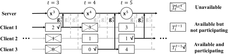
Figure 1. A simple illustration of FedLaAvg. The cloud server chooses $K=1$ client with the most outdated gradient from the available clients to participate in each iteration. The black lines between iterations mean the chosen client participates in this iteration and uploads its current gradient, while the grey dotted lines mean the cloud server uses the absent client’s latest gradient in this iteration. Number $T^{t-1}_{i}$ in the rectangles denotes the latest iteration in which the client $i$ participates.

We present in Algorithm 1 the detailed procedures of FedLaAvg, and give Figure 1 for easy illustration. In each iteration $t$, each selected client $i$ locally calculates the gradient $\mathbf{g}^{t}_{i}$, and the cloud server maintains the average latest gradient $\mathbf{g}^{t}$ of all clients. The client selection principle in FedLaAvg is to choose the $K$ clients that are absent from the training process for the longest time from the available clients (Lines 5–7). Together with Assumption 4, we can guarantee that each client is selected at least once during any period with $I$ successive iterations, where $I$ is a function of parameters $K$, $N$, and $E$ (please refer to Lemma 2 in Section 4 for the details). Based on this condition, we can establish an upper bound for the difference between each client’s latest gradient and its current gradient, which would be critical for the convergence analysis of FedLaAvg in Section 4. To implement this principle, we use $T^{t}_{i}$ to record the latest iteration before or at $t$ in which client $i$ participates in the training process. During the aggregation procedure (Lines 8–9), to reduce the aggregation overhead, each selected client uploads the gradient difference: the difference between the gradients computed in the current participating iteration and the previous participating iteration, i.e., $\mathbf{g}^{t}_{i}-\mathbf{g}^{T^{t-1}_{i}}_{i}$, rather than the current gradient $\mathbf{g}^{t}_{i}$ as in the traditional FedAvg algorithm. Once the gradient difference from each client $i$ is received, the cloud server would update the global gradient (Line 9). Following this aggregation method, the cloud server only needs to store the average latest gradient $\mathbf{g}^{t}$ and run $K$ update operations. It can be proved by induction that at the end of each iteration $t$, the resulting gradient is indeed the average latest gradient:

(3) $$\mathbf{g}^{t}=\frac{1}{N}\sum_{i=1}^{N}\mathbf{g}^{T^{t}_{i}}_{i}.$$

Once the average latest gradient $\mathbf{g}^{t}$ is obtained, the cloud server uses it to update the global model parameters in (4).

Algorithm 1 Federated Latest Averaging Algorithm

1:  Input: initial model parameters $\mathbf{x}^{0}$; number of clients $N$; number of total iterations $T$; learning rate $\gamma$; proportion of selected clients $\beta$ (i.e., the number of participating clients in each iteration is $K=\beta N$.)

2:  Initialization: $\mathbf{g}^{0}\leftarrow\mathbf{0};\,\forall i\in\{1,2,\cdots,N\},\,\mathbf{g}_{i}^{0}\leftarrow\mathbf{0},\,T_{i}^{0}\leftarrow 0$.

3:  for $t=1$ to $T$ do

4:     $\mathbf{g}^{t}\leftarrow\mathbf{g}^{t-1}$

5:     $\mathcal{C}^{t}\leftarrow$ the set of available clients

6:     $\mathcal{B}^{t}\leftarrow$ $K$ clients from $\mathcal{C}^{t}$ with the lowest $T^{t-1}_{i}$ values

7:     Update $T^{t}_{i}$ values: $T^{t}_{i}\leftarrow t,\,\forall i\in\mathcal{B}^{t};\;T^{t}_{i}\leftarrow T^{t-1}_{i},\,\forall i\notin\mathcal{B}^{t}.$

8:     Each client $i\in\mathcal{B}^{t}$ calculates local gradient $\mathbf{g}^{t}_{i}$ and uploads gradient difference $\mathbf{g}^{t}_{i}-\mathbf{g}^{T^{t-1}_{i}}_{i}$.

9:     Once receiving the gradient information from client $i$, the cloud server calculates the global gradient:

$$\mathbf{g}^{t}\leftarrow\mathbf{g}^{t}+\frac{1}{N}\left(\mathbf{g}^{t}_{i}-\mathbf{g}^{T^{t-1}_{i}}_{i}\right).$$

10:     The cloud server updates the global model parameters:

(4) $$\mathbf{x}^{t}\leftarrow\mathbf{x}^{t-1}-\gamma\mathbf{g}^{t}.$$

11:  end for

4. Convergence Analysis

In this section, under intermittent client availability, we show that FedLaAvg achieves $O(E^{1/2}/(N^{1/4}T^{1/2}))$ convergence rate on general non-convex functions with a sublinear speedup in terms of the total number of clients.

4.1. Convergence on Example 1

We first demonstrate that FedLaAvg converges in Example 1, where FedAvg produces an arbitrarily poor-quality result. The convergence analysis of FedLaAvg for this simple example sheds light on the analysis for the case of general non-convex optimization in the next subsection.

Theorem 1.

Suppose each client computes the exact (not stochastic) gradient. In Example 1, after $T$ iterations, FedLaAvg with the learning rate $\gamma=1/(2\sqrt{T})$ produces a solution $\hat{\mathbf{x}}$ that is within $O(1/\sqrt{T})$ range of the optimal solution $\mathbf{x}^{*}$: $\left(\hat{\mathbf{x}}-\mathbf{x}^{*}\right)^{2}=O(1/\sqrt{T}),$ where we choose $\hat{\mathbf{x}}=\arg\min_{\mathbf{x}^{t}}f(\mathbf{x}^{t})$ as the output.

Proof of Theorem 1.

We recall that

$$f(\mathbf{x})=\left(\mathbf{x}-\frac{\mathbf{e}_{1}+\mathbf{e}_{2}}{2}\right)^{2}+\frac{\left(\mathbf{e}_{1}-\mathbf{e}_{2}\right)^{2}}{4}+\frac{1}{2}\sum_{i=1}^{2}\mathbb{E}_{\xi_{i}\sim\mathcal{D}_{i}}\left[(\xi_{i}-\mathbf{e}_{i})^{2}\right],$$

where the latter two terms are not associated with the variable $\mathbf{x}$. Hence, we only need to focus on the following part of the loss function: $\hat{f}(\mathbf{x})=\left(\mathbf{x}-\mathbf{x}^{*}\right)^{2},$ where $\mathbf{x}^{*}=\frac{\mathbf{e}_{1}+\mathbf{e}_{2}}{2}$ is the optimal solution. Note that

(5) $$\hat{f}(\mathbf{x}^{t})-\hat{f}(\mathbf{x}^{t-1})=\left(\mathbf{x}^{t}-\mathbf{x}^{t-1}\right)^{2}+2\left(\mathbf{x}^{t-1}-\mathbf{x}^{*}\right)\left(\mathbf{x}^{t}-\mathbf{x}^{t-1}\right).$$

We calculate the difference of $\mathbf{x}$ between two successive iterations:

$$\mathbf{x}^{t}-\mathbf{x}^{t-1} =-\frac{\gamma}{2}\left(\mathbf{g}_{1}^{T^{t}_{1}}+\mathbf{g}_{2}^{T^{t}_{2}}\right)=-\gamma\left(\mathbf{x}^{T^{t}_{1}}-\mathbf{e}_{1}+\mathbf{x}^{T^{t}_{2}}-\mathbf{e}_{2}\right)$$

(6) $$=-\gamma\left(\mathbf{x}^{T^{t}_{1}}+\mathbf{x}^{T^{t}_{2}}-2\mathbf{x}^{*}\right),$$

where $T^{t}_{i}$ is defined in Section 3.2. Hence, we have

$$2\left(\mathbf{x}^{t-1}-\mathbf{x}^{*}\right)\left(\mathbf{x}^{t}-\mathbf{x}^{t-1}\right)$$

$$= -\gamma\left(2\mathbf{x}^{t-1}-2\mathbf{x}^{*}\right)\left(\mathbf{x}^{T^{t}_{1}}+\mathbf{x}^{T^{t}_{2}}-2\mathbf{x}^{*}\right)$$

$$= -\frac{\gamma}{2}\left(2\mathbf{x}^{t-1}-2\mathbf{x}^{*}\right)^{2}-\frac{\gamma}{2}\left(\mathbf{x}^{T^{t}_{1}}+\mathbf{x}^{T^{t}_{2}}-2\mathbf{x}^{*}\right)^{2}$$

(7) $$+\frac{\gamma}{2}\left(2\mathbf{x}^{t-1}-\mathbf{x}^{T^{t}_{1}}-\mathbf{x}^{T^{t}_{2}}\right)^{2}.$$

Substituting (4.1) and (4.1) into (5), we have

(8) $$\hat{f}(\mathbf{x}^{t})-\hat{f}(\mathbf{x}^{t-1})\leq-2\gamma\left(\mathbf{x}^{t-1}-\mathbf{x}^{*}\right)^{2}+\frac{\gamma}{2}\left(2\mathbf{x}^{t-1}-\mathbf{x}^{T^{t}_{1}}-\mathbf{x}^{T^{t}_{2}}\right)^{2},$$

which follows from $0<\gamma\leq 1/2$.

The algorithm starts from model parameters $\mathbf{x}^{0}$. When client $1$ is available, $\mathbf{x}$ moves towards $\mathbf{e}_{1}$, and when client $2$ is available, $\mathbf{x}$ moves towards $\mathbf{e}_{2}$. Hence, $\mathbf{x}$ is always within $G/2$ range of $\mathbf{x}^{*}$:

(9) $$-\frac{G}{2}\leq\mathbf{x}^{t}-\mathbf{x}^{*}\leq\frac{G}{2},\,\forall t\geq 0,$$

where $G=\max\left\{2\left(\mathbf{x}^{0}-\mathbf{x}^{*}\right),\left\lvert\mathbf{e}_{1}-\mathbf{e}_{2}\right\rvert\right\}$ is the the largest gradient norm during the training process. Substituting (9) into (4.1), we have

(10) $$-\gamma G\leq\mathbf{x}^{t}-\mathbf{x}^{t-1}\leq\gamma G.$$

Referring to the specific client availability model in this example, we have $t-T^{t}_{i}\leq I=\max\left\{t_{1},t_{2}\right\}$, $i=1,\,2$. Therefore, when $t\geq T^{t}_{i}+2$, summing (10) over iterations from $T^{t}_{i}+1$ to $t-1$, we have

(11) $$-\gamma IG\leq\mathbf{x}^{t-1}-\mathbf{x}^{T^{t}_{i}}\leq\gamma IG,\,i=1,\,2.$$

Note that when $t=T^{t}_{i}$ or $t=T^{t}_{i}+1$, the above formula also holds.

Substituting (11) into (8), we have

$$\hat{f}(\mathbf{x}^{t})-\hat{f}(\mathbf{x}^{t-1})\leq-2\gamma\left(\mathbf{x}^{t-1}-\mathbf{x}^{*}\right)^{2}+2\gamma^{3}I^{2}G^{2}.$$

Rearranging the formula, we have

$$\left(\mathbf{x}^{t-1}-\mathbf{x}^{*}\right)^{2}\leq\frac{1}{2\gamma}\left(\hat{f}(\mathbf{x}^{t-1})-\hat{f}(\mathbf{x}^{t})\right)+\gamma^{2}I^{2}G^{2}.$$

Summing this inequility over iterations from 1 to $T$, we have

$$\frac{1}{T}\sum_{t=1}^{T}\left(\mathbf{x}^{t-1}-\mathbf{x}^{*}\right)^{2} \leq\frac{1}{2\gamma T}\left(\hat{f}(\mathbf{x}^{0})-\hat{f}(\mathbf{x}^{T})\right)+\gamma^{2}I^{2}G^{2}$$

(12) $$\leq\frac{1}{2\gamma T}\left(\hat{f}(\mathbf{x}^{0})-\hat{f}(\mathbf{x}^{*})\right)+\gamma^{2}I^{2}G^{2}.$$

Substituting $\gamma=1/(2\sqrt{T})$ into (4.1), we have

$$\frac{1}{T}\sum_{t=1}^{T}\left(\mathbf{x}^{t-1}-\mathbf{x}^{*}\right)^{2} \leq\frac{1}{\sqrt{T}}\left(\hat{f}(\mathbf{x}^{0})-\hat{f}(\mathbf{x}^{*})\right)+\frac{I^{2}G^{2}}{4T}$$

$$=\frac{1}{\sqrt{T}}\left(f(\mathbf{x}^{0})-f(\mathbf{x}^{*})\right)+\frac{I^{2}G^{2}}{4T}.$$

Finally, we have

$$\left(\hat{\mathbf{x}}-\mathbf{x}^{*}\right)^{2}\leq\frac{1}{T}\sum_{t=1}^{T}\left(\mathbf{x}^{t-1}-\mathbf{x}^{*}\right)^{2}$$

$$\leq \frac{1}{\sqrt{T}}\left(f(\mathbf{x}^{0})-f(\mathbf{x}^{*})\right)+\frac{I^{2}G^{2}}{4T}=O\left(\frac{1}{\sqrt{T}}\right).$$

∎

4.2. Convergence on General Non-Convex Functions

In this subsection, we show the $O(E^{1/2}/(N^{1/4}T^{1/2}))$ convergence of FedLaAvg on general non-convex functions. First, we introduce Lemma 2 about client participation.

Lemma 0.

Under Assumption 4, the client selection policy in FedLaAvg guarantees that for each client, the latest participating iteration is at most $I$ iterations earlier than the current iteration: $t-T^{t}_{i}\leq I,\,\forall t,\,\forall i,\,\text{where}\,I=\left\lceil\frac{N}{K}\right\rceil E-1$

Proof of Lemma 2.

Please refer to Appendix B.1. ∎

With such a client participation condition, we can derive a key result for analyzing the convergence of FedLaAvg.

Theorem 3.

By setting $\gamma\leq 1/(2L)$ in FedLaAvg, we can derive the following bound on the average expected squared gradient norm under Assumptions 1–4:

$$\frac{1}{T}\sum_{t=1}^{T}\mathbb{E}\left[\left\lVert\nabla f(\mathbf{x}^{t-1})\right\rVert^{2}\right]$$

$$\leq \underbrace{\frac{2\gamma IL\left(G^{2}+\sigma^{2}\right)}{\sqrt{N}}+\frac{2\gamma^{2}I^{2}L^{2}G^{2}}{1-2\gamma L}+4\gamma^{2}I^{2}L^{2}G^{2}}_{\text{gradient staleness}}$$

$$+\underbrace{\frac{4\gamma\sigma^{2}L}{N}}_{\text{gradient variance}}+\underbrace{\frac{4}{\gamma T}\left(\mathbb{E}\left[f(\mathbf{x}^{0})\right]-\mathbb{E}\left[f(\mathbf{x}^{*})\right]\right)}_{\text{objective distance}},$$

where $\mathbf{x}^{*}$ is the the optimal solution for the general non-convex optimization problem.

Proof Sketch of Theorem 3.

Based on Assumption 1 about smoothness, we decompose the difference of the loss function values in two successive iterations, i.e., $\mathbb{E}[f(\mathbf{x}^{t})]-\mathbb{E}[f(\mathbf{x}^{t-1})]$, into several terms. With Lemma 2, we show that the gradient staleness, i.e., difference between the latest gradient and the corresponding current gradient, is bounded. With Assumption 3, we show that the error related to stochastic gradient variance is also bounded. With the gradient staleness bound and the gradient variance bound, we further prove an upper bound for each decomposed term mentioned above. Finally, we prove the theorem by summing up the bounds over iterations $t$ from $1$ to $T$ and rearranging the resulted inequation. For the detailed proof, please refer to Appendix B.2. ∎

Before presenting our main result, we consider the full client participation setting discussed in Yu et al. (2019b), in which our FedLaAvg reduces to FedAvg. Since $K=N$, $E=1$, and $I=\lceil N/K\rceil E-1=0$ in this setting, the gradient staleness term vanishes and the result in Theorem 3 becomes

$$\frac{1}{T}\sum_{t=1}^{T}\mathbb{E}\left[\left\lVert\nabla f(\mathbf{x}^{t-1})\right\rVert^{2}\right]\leq\frac{4\gamma\sigma^{2}L}{N}+\frac{4}{\gamma T}\left(\mathbb{E}\left[f(\mathbf{x}^{0})\right]-\mathbb{E}\left[f(\mathbf{x}^{*})\right]\right).$$

Choosing $\gamma=\sqrt{N}/(2L\sqrt{T})$, when $T\geq N$, we can obtain the $O(1/\sqrt{NT})$ convergence, which is consistent with the linear speedup in terms of $N$ as proven in Yu et al. (2019b).

For the intermittent client availability setting considered in this work, FedLaAvg achieves a sublinear speedup by choosing appropriate hyperparameters. For easy illustration, we define the loss difference between the initial solution $\mathbf{x}^{0}$ and the optimal solution $\mathbf{x}^{*}$ as $B=f(\mathbf{x}^{0})-f(\mathbf{x}^{*})$. In addition, we recall that $\beta=K/N$ is the proportion of the selected clients in each iteration.

Corollary 0.

By choosing the learning rate $\gamma=\frac{\beta^{\frac{1}{2}}N^{\frac{1}{4}}}{2LE^{\frac{1}{2}}T^{\frac{1}{2}}}$ and requiring $\gamma\leq 1/(4L)$ in FedLaAvg, we have the following convergence result:

$$\frac{1}{T}\sum_{t=1}^{T}\mathbb{E}\left[\left\lVert\nabla f(\mathbf{x}^{t-1})\right\rVert^{2}\right]=O\left(\frac{E^{\frac{1}{2}}\left(G^{2}+\sigma^{2}+LB\right)}{N^{\frac{1}{4}}T^{\frac{1}{2}}\beta^{\frac{1}{2}}}+\frac{EG^{2}N^{\frac{1}{2}}}{T\beta}\right).$$

When $T\geq EN^{3/2}/\beta$, we further obtain the sublinear speedup with respect to the total number of clients:

$$\frac{1}{T}\sum_{t=1}^{T}\mathbb{E}\left[\left\lVert\nabla f(\mathbf{x}^{t-1})\right\rVert^{2}\right]=O\left(\frac{E^{\frac{1}{2}}\left(G^{2}+\sigma^{2}+LB\right)}{N^{\frac{1}{4}}T^{\frac{1}{2}}\beta^{\frac{1}{2}}}\right)=O\left(\frac{E^{\frac{1}{2}}}{N^{\frac{1}{4}}T^{\frac{1}{2}}}\right).$$

Proof of Corollary 4.

Please refer to Appendix B.3. ∎

5. Extension to Communication Round-Based Setting

In practical FL deployment, for communication efficiency, each participating client is allowed to perform multiple local training iterations before uploading the accumulated local model update in each communication round (McMahan et al., 2017). Although we focused in earlier sections on the case where participating clients communicate every iteration, FedLaAvg can be trivially extended to support multiple local iterations per communication round.

Algorithm 2 The Communication Round-Based Federated Latest Averaging Algorithm

1:  Input: initial model parameters $\mathbf{x}^{0}$; number of clients $N$; number of total rounds $R$; learning rate $\gamma$; number of local iterations $C$; proportion of selected clients $\beta$ (i.e., the number of participating clients in each round is $K=\beta N$.)

2:  Do initialization:

$$\mathbf{u}^{0}\leftarrow\mathbf{0},\,\forall i\in\{1,2,\cdots,N\},\,\mathbf{u}_{i}^{0}\leftarrow\mathbf{0},\,R_{i}^{0}\leftarrow 0.$$

3:  for $r=1$ to $R$ do

4:     $\mathbf{u}^{r}\leftarrow\mathbf{u}^{r-1}$

5:     $\hat{\mathcal{C}}^{r}\leftarrow$ the set of available clients

6:     $\hat{\mathcal{B}}^{r}\leftarrow$ $K$ clients from $\hat{\mathcal{C}}^{r}$ with the lowest $R_{i}^{r-1}$ values

7:     Update $R_{i}^{r}$ values:

$$R_{i}^{r}\leftarrow r,\,\forall i\in\hat{\mathcal{B}}^{r};\,R_{i}^{r}\leftarrow R_{i}^{r-1},\,\forall i\notin\hat{\mathcal{B}}^{r}.$$

8:     Each client $i\in\hat{\mathcal{B}}^{r}$ calculates the accumulated local model update $\mathbf{u}_{i}^{r}$ and uploads the update difference $\mathbf{u}_{i}^{r}-\mathbf{u}_{i}^{R_{i}^{r-1}}$ in parallel.

9:     Once receiving the update information from client $i$, the cloud server calculates the global update:

$$\mathbf{u}^{r}\leftarrow\mathbf{u}^{r}+\frac{1}{N}\left(\mathbf{u}_{i}^{r}-\mathbf{u}_{i}^{R_{i}^{r-1}}\right).$$

10:     The cloud server updates the global model parameters:

$$\mathbf{x}^{rC}\leftarrow\mathbf{x}^{rC-C}+\mathbf{u}^{r}.$$

11:  end for

We introduce some notations to represent the training process of the communication round-based FedLaAvg. $C$ denotes the local iteration number. Let $\hat{\mathcal{C}}^{r}\triangleq\bigcap_{t=(r-1)C+1}^{rC}\mathcal{C}^{t}$ be the set of available clients in round $r$. Each client $i$ observes the stochastic gradient $\mathbf{g}^{t}_{i}$ on the local model parameters in each local iteration, and accumulates these stochastic gradients to obtain the local model update $\mathbf{u}_{i}^{r}\triangleq-\gamma\sum_{t=(r-1)C+1}^{rC}\mathbf{g}^{t}_{i}$ in round $r$. After collecting the local model updates at the end of round $r$, (i.e., in iteration $t=rC$), the cloud server calculates the global model parameters $\mathbf{x}^{rC}$. Similar to the notation $T^{t}_{i}$, we use $R_{i}^{r}$ to denote the latest round where client $i$ is available before or in round $r$. We define $r^{t}\triangleq\lfloor(t-1)/C\rfloor+1$ as the round that iteration $t$ belongs to. The one-iteration-per-round scenario corresponds to the special case using the specific notations: $C=1$, $r^{t}=t$, $\hat{\mathcal{C}}^{r^{t}}=\mathcal{C}^{t}$, $\mathbf{u}_{i}^{r^{t}}=-\gamma\mathbf{g}^{t}_{i}$, and $R_{i}^{r^{t}}=T^{t}_{i}$.

To apply FedLaAvg to the multiple-iteration-per-round scenario, we need only replace the cached gradient $\mathbf{g}^{t}$ in Algorithm 1 with cached update $\mathbf{u}^{r}$. The communicated gradient difference $\mathbf{g}^{t}_{i}-\mathbf{g}^{T^{t-1}_{i}}_{i}$ is replaced with the update difference $\mathbf{u}_{i}^{r}-\mathbf{u}_{i}^{R_{i}^{r-1}}$. The algorithm is formally presented in Algorithm 2.

As we consider multiple local iterations per communication round, client availability should be measured in rounds. Hence we replace Assumption 4 with Assumption 5:

Assumption 5.

Minimal availability: each client $i$ is available at least once in any period with $E$ successive rounds:

$$\forall i,\,\forall r,\,\exists\hat{r}\in\{r,r+1,\cdots,r+E-1\},\text{ such that }i\in\hat{\mathcal{C}}^{\hat{r}}.$$

Under Assumption 5, we can establish the following convergence rate of the extended algorithm:

Theorem 1.

We recall that $B=f(\mathbf{x}^{0})-f(\mathbf{x}^{*})$ and $\beta=K/N$. Let the communication round-based FedLaAvg execute $R$ rounds. By choosing the learning rate $\gamma=(\beta^{1/2}N^{1/4})/(2LCE^{1/2}R^{1/2})$ and requiring $\gamma\leq 1/(4L)$, we have the following convergence result:

$$\frac{1}{R}\sum_{r=1}^{R}\mathbb{E}\left[\left\lVert\nabla f(\mathbf{x}^{rC-1})\right\rVert^{2}\right]=O\left(\frac{E^{\frac{1}{2}}\left(G^{2}+\sigma^{2}+LB\right)}{N^{\frac{1}{4}}R^{\frac{1}{2}}\beta^{\frac{1}{2}}}+\frac{EG^{2}N^{\frac{1}{2}}}{R\beta}\right).$$

When $R\geq EN^{3/2}/\beta$, we further have

$$\frac{1}{R}\sum_{r=1}^{R}\mathbb{E}\left[\left\lVert\nabla f(\mathbf{x}^{rC-1})\right\rVert^{2}\right]=O\left(\frac{E^{\frac{1}{2}}\left(G^{2}+\sigma^{2}\right)+BL}{\beta^{\frac{1}{2}}N^{\frac{1}{4}}R^{\frac{1}{2}}}\right)=O\left(\frac{E^{\frac{1}{2}}}{N^{\frac{1}{4}}R^{\frac{1}{2}}}\right).$$

Proof of Theorem 1.

Please refer to Appendix C. ∎

6. Experiments

In this section, we evaluate the performance of FedLaAvg in different tasks, datasets, models, and availability settings.

6.1. Experimental Setups

6.1.1. Federated learning tasks.

We choose the following two tasks for evaluation.

Image classification. We first take an image classification task over the MNIST dataset (LeCun et al., 1998), to validate the convergence of FedLaAvg, and the divergence of FedAvg even in a simple convex setting. The dataset consists of 70000 28$\times$28 grey images of hand-written digits, where 60000 images are for training and the other 10000 ones are for testing. In this task, we adopt the multinomial logistic regression model, which has a convex optimization objective. To simulate non-IID data distribution, we set each client to hold only images of one certain digit, and the number of clients holding the same digit to be $N/10$. To simulate data unbalance, we let the number of samples on each client roughly follow a normal distribution with mean $6\times 10^{4}/N$ and variance $(1\times 10^{4}/N)^{2}$.

Sentiment analysis. In the general non-convex case, we take a binary text sentiment classification task on the Sentiment140 dataset (Go et al., 2009). The dataset consists of 1600000 tweets collected from 659775 twitter users. In this task, we use a two-layer LSTM binary classifier with 16 hidden units and pretrained 25D GloVe embeddings (Pennington et al., 2014) as the classification model. We naturally partition this dataset by letting each Twitter account correspond to a client. We keep only the clients who hold more than 40 samples and get 1473 clients, and randomly select one-tenth of the data as the test dataset.

Figure 2. The availability setting with diurnal pattern adopted in the MNIST experiments. Clients holding digits $0,\cdots,D-1$ are available in white grids, while the remaining clients are available in black grids.

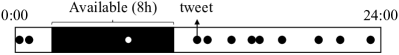
Figure 3. The availability setting adopted in the Sentiment140 experiments. The black or white dots denote that the client sent a tweet at this moment one day.

(a) Legends

(b) $E=100$, $D=3$

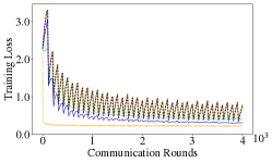
(c) $E=100$, $D=5$

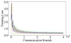
(d) $E=50$, $D=1$

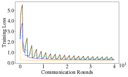
(e) $E=100$, $D=1$

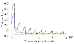
(f) $E=200$, $D=1$

Figure 4. Training losses of FedSGD, FedAvg, FedProx, FedLaAvg, and sequential SGD in the MNIST image classification task with different client availability settings.

6.1.2. Baselines

We choose the following baselines for comparison.

FedAvg and FedSGD. FedAvg was proposed by the seminal work of FL (McMahan et al., 2017), which naively uses the average of the collected local model updates to update the global model. FedSGD is a special case of FedAvg with only one local iteration.

FedProx. FedProx (Li et al., 2020b) is the first variant of FedAvg with guaranteed convergence while allowing partial client participation. The main modification to FedAvg is that FedProx adds a quadratic proximal term to explicitly limit the local model updates. We follow the practice of the original work (Li et al., 2020b) to set the proxy term coefficient as 1.0 for MNIST and 0.01 for Sentiment140.

Sequential SGD. We run the standard SGD algorithm to train the global model using the whole dataset, and set the total number of iterations in each round as $\beta NC$. This ensures the same amount of computation per round with the distributed algorithms. The result of sequential SGD can be regarded as the ideal solution for the optimization problem.

6.1.3. Availability Settings and Other Settings

We simulate the client availability as follows.

In the MNIST image classification experiments, we adopt the typical subcase of our intermittent client availability model with the diurnal pattern (Bonawitz et al., 2019; Yang et al., 2018; Eichner et al., 2019), depicted in Figure 2. In the white grids, the clients holding digits $0,1,\cdots,D-1$ are available for $E$ rounds, and in the black grids, the remaining clients are available for the next $E$ rounds. This setting captures that the client availability correlates with the local data distribution in practice, and $D$ controls the degree of such availability heterogeneity.

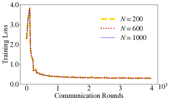
(a) Training loss with different $N$

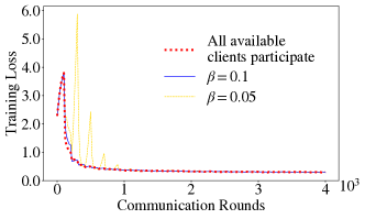
(b) Training loss with different $\beta$

Figure 5. Training losses of FedLaAvg on MNIST dataset by varying the total number of clients $N$ and the proportion of selected clients $\beta$.

(a) Legends

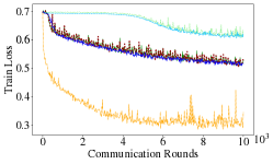
(b) $E=120$, $\alpha=0.25$

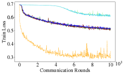
(c) $E=120$, $\alpha=0.5$

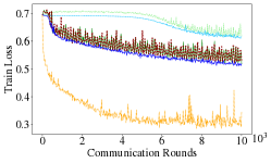
(d) $E=24$, $\alpha=0$

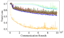
(e) $E=120$, $\alpha=0$

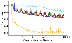
(f) $E=240$, $\alpha=0$

Figure 6. Training losses of FedSGD, FedAvg, FedProx, FedLaAvg, and sequential SGD in the Sentiment140 sentiment analysis task with different client availability settings.

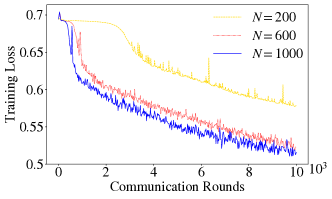
(a) Training loss with different $N$

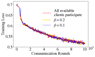
(b) Training loss with different $\beta$

Figure 7. Training losses of FedLaAvg on Sentiment140 dataset by varying the total number of clients $N$ and the proportion of selected clients $\beta$.

In the sentiment analysis experiments over Sentiment140, we assume that clients are available only when the Twitter users are sleeping, such that the devices are idle and eligible for the model training. Hence, we set each client to be available for eight hours each day, during which the client sends the least number of tweets, as illustrated in Figure 3. To capture the correlation of client availability and local data distribution in practical FL, we vary the label balance as a function of the time of day. In particular, we randomly drop tweets sent in 0:00–1:00 such that $\alpha$ proportion of tweets are positive sentiment; we randomly drop tweets sent in 12:00-13:00 such that $1-\alpha$ proportion of tweets are positive sentiment; and we linearly interpolate for other hours of day.

As the default experiment settings, we set the total number of clients $N=1000$, the period length $E=100$ for MNIST and $E=120$ for Sentiment140, the availability heterogeneity controlling parameter $D=1$ for MNIST and $\alpha=0.0$ for Sentiment140, the proportion of selected clients in each round $\beta=0.1$, and the number of local iterations $C=10$. For hyperparameters, we set the learning rate to $0.01$, and the local batch size to $5$ for MNIST and $2$ for Sentiment140, respectively.

6.2. Results in the Convex Case

We first compare FedLaAvg with the aforementioned baselines in the MNIST image classification task under various availability settings. In particular, we vary $E$ from $50$ to $200$, which controls the maximum number of unavailable rounds, and vary $D$ from 1 to 5, which controls the differentiation of client availability. We show the results in Figure 4. In general, we observe that FedLaAvg converges in approximately 2000 rounds under all the five availability settings. In addition, FedLaAvg approaches sequential SGD in terms of training loss. These coincide with Theorem 3. In contrast, FedSGD, FedAvg, and FedProx suffer from periodic osillation in any availability setting, especially when either $E$ or $D$ is large, which validates Theorem 2. By comparing FedProx and FedAvg, we can see that the training losses of these two algorithms almost overlap, which indicates that FedProx also cannot solve the issue of intermittent client availablity. By comparing FedLaAvg with one and multiple local iterations, we find that introducing multiple local iterations speeds up the convergence with respect to communication rounds in practice.

We then evaluate the effect of the total number of clients $N$ and the proportion of selected clients $\beta$ on FedLaAvg in Figure 5. From Figure 5(a), we can see that FedLaAvg with different $N$ behaves almost uniformly. This is because a larger $N$ improves the convergence by reducing the variance of the global model update, while for such a simple convex training scenario, the variance is already small enough with $N=200$. From Figure 5(b), we observe that selecting more clients in each round leads to more stable training, but after reaching a certain threshold, selecting further more clients would not help much.

6.3. Results in the Non-Convex Case

We next evaluate FedLaAvg and the baselines over the Sentiment140 dataset. First, we compare different algorithms under various availability settings in Figure 6. In particular, we vary $E$ from 24 to 240, and vary $\alpha$ from 0 to 0.5, which controls the differentiation of client availability. Similar to the convex case, FedLaAvg converges in all the five availability settings, while FedSGD, FedAvg, and FedProx suffer from severe oscillation, especially when either $E$ is large or $\alpha$ is small; FedProx still cannot solve the issue of intermittent client availability. We note that $\alpha=0.5$ indicates that the ratio of positive tweets is fixed at $0.5$ throughout the training process. There is nearly no correlation between client availability and local data distribution in this setting, and thus the performance of FedAvg is similar to that of FedLaAvg. In addition, we observe that introducing multiple local iterations to FedLaAvg significantly speeds up the convergence, which further validates the empirical communication efficiency improvement of local iterations.

We finally evaluate the impacts of the total number of clients $N$ and the proportion of selected clients $\beta$ on FedLaAvg, and show the results in Figure 7. From Figure 7(a), we observe that FedLaAvg with a larger $N$ converges much faster, which validates the sublinear speedup with respect $N$. From Figure 7(b), we can see that $\beta$ has little effect on the convergence of FedLaAvg in this task.

For all the experiments above, we also show the test accuracies with training rounds in Appendix E, which behave consistently with the training losses.

7. Conclusion

In this work, we investigate intermittent client availability in FL and its impact on the convergence of the classical FedAvg algorithm. We use a collection of time-varying sets to represent the available clients in each training iteration, which can accurately model the intermittent client availability. Furthermore, we design a simple FedLaAvg algorithm with an $O(E^{1/2}/(N^{1/4}T^{1/2}))$ convergence guarantee for general distributed non-convex optimization problems. Empirical studies with the standard MNIST and Sentiment140 datasets demonstrate the effectiveness and efficiency of FedLaAvg with a remarkable performance improvement and a sublinear speedup.

Appendix A Divergence of the concurrent work under intermittent client availability

The concurrent work (Ruan et al., 2020) considered a different availability setting, where the number of local iterations performed by client $i$ in round $r$ can take an arbitrary value $s_{r}^{i}$ from $\{0,1,\cdots,C\}$, following some time-varying distribution. For the clients submitting incompleted work, i.e., $1\leq s_{r}^{i}<C$, they proposed to scale the model update by $w_{i}^{r}=\frac{C}{s_{i}^{r}}w_{i}$, to force equal contribution to the global model among clients. Under this framework, they proved the convergence, which, however, is tailed with a bias term $\frac{M_{R}}{R}$; $R$ is the total number of communication rounds, and $M_{R}$ represents the accumulated training data bias throughout the training process. Specifically, $M_{R}=\sum_{r=1}^{R}\mathbb{E}\left[z_{r}\right]$, where $z_{r}=0$ if all clients contribute equally to the global model update in round $r$, i.e., $\frac{\mathbb{E}\left[w_{i}^{r}s_{i}^{r}\right]}{w_{i}}$ take the same value for all clients $i$, and $z_{r}=1$ else. When there exists a single client $i$ whose $s_{r}^{i}=0$ with probability $p_{i}>0$, i.e., client $i$ is unavailable in round $r$, the proposed scaling technique cannot work and $z_{r}=p_{i}$. Further, if there exists multiple clients whose $s_{r}^{i}=0$ with probability $p_{i}>0$, $z_{r}$ is even larger. The work (Ruan et al., 2020) claims that their method converges if $M_{R}$ increases sublinearly with $R$.

The proposed method works mainly in the scenario that in most rounds of training, there are no unavailable clients. However, under intermittent client availability considered in this work, there exist unavailable clients in almost every round. E.g., in our Example 1, two clients are available alternately, and there is always one client unavailable throughout the training process, i.e., $s_{i}^{r}=1$ with probability $1$, indicating that $M_{R}=R$ and the method diverges. Further, the work (Ruan et al., 2020) proposed to kick out frequently unavailable clients if the evaluated training data bias introduced by keeping the clients, i.e., $\frac{M_{R}}{R}$, is larger than that introduced by kicking the clients out. This, however, still cannot solve the bias problem, since the bias always exists no matter whether frequently unavailable clients are kicked out or not.

Appendix B Detailed Proof of the Convergence of FedLaAvg

B.1. Proof of Lemma 2

Proof of Lemma 2.

$\forall t,\forall i$, we focus on the training process from $t$ (not included). In iteration $t+I+1$, under Assumption 4, client $i$ has been available for at least $\lceil N/K\rceil$ times. Note the $\lceil N/K\rceil$ iterations as $\tau_{1},\tau_{2},\cdots,\tau_{\lceil N/K\rceil}$. We prove the lemma by contradiction. Suppose $i$ is not selected in any of these iterations. Then we have $T_{i}^{\tau_{\lceil N/K\rceil}}=T^{t}_{i}$. In the $\lceil N/K\rceil$ iterations where client $i$ is available, $\lceil N/K\rceil K$ clients have been selected. All these clients (noted as $j$) are with $T_{j}^{\tau}\leq T^{t}_{i}$ for all iterations $\tau$ before it participates in the training process and $T_{j}^{\tau}>T^{t}_{i}$ for all iterations $\tau$ after participation. Hence, the $\lceil N/K\rceil K$ clients are distinct. Including client $i$, the system has at least $\lceil N/K\rceil K+1$ clients. However, the system has only $N\leq\lceil N/K\rceil K<\lceil N/K\rceil K+1$ clients. This forms a contradiction. Therefore, for all $t$, the next iteration $t_{next}$ where $i$ participates in the training process after iteration $t$ satisfies

(13) $$t_{next}\leq t+I+1.$$

For all client $i$, by setting $t$ to iterations where client $i$ is selected in (13), we can derive

$$\forall i,\>\forall t,\>t-T^{t}_{i}\leq I.$$

∎

B.2. Proof of Theorem 3

Note that local gradient is not calculated in each iteration. In this subsection of the appendix, for mathematical analysis, we extend the definition $\mathbf{g}^{t}_{i}\triangleq\nabla F(\mathbf{x}^{t-1},\xi_{i}^{t})$. For iterations where client $i$ does not participate, $\xi_{i}^{t}$ is a random variable which follows $\xi_{i}^{t}\sim\mathcal{D}_{i}$.

Lemma 0.

Under Assumption 2 and 3, we have

$$\mathbb{E}\left[\left\lVert\mathbf{g}^{t}_{i}\right\rVert^{2}\right]\leq G^{2},\forall i,\forall t$$

and

$$\mathbb{E}\left[\left\lVert\mathbf{g}^{t}_{i}-\nabla f_{i}(\mathbf{x}^{t-1})\right\rVert^{2}\right]\leq\sigma^{2},\forall i,\forall t.$$

Proof of Lemma 1.

Our Assumptions 2 and 3 take the expectation over the randomness of one training iteration. But we care about the expectation taken over the randomness of the whole training process. This trivial lemma builds the gap.

For the gradient, we have

(14) $$\mathbb{E}\left[\left\lVert\mathbf{g}^{t}_{i}\right\rVert^{2}\right]\overset{(a)}{=}\mathbb{E}\left[\mathbb{E}\left[\left\lVert\mathbf{g}^{t}_{i}\right\rVert^{2}\mid\xi^{[t-1]}\right]\right]=\mathbb{E}\left[\mathbb{E}\left[\left\lVert\nabla F\left(\mathbf{x}^{t-1},\xi_{i}^{t}\right)\right\rVert^{2}\mid\mathbf{x}^{t-1}\right]\right]\overset{(b)}{\leq}\mathbb{E}\left[G^{2}\right]=G^{2},$$

where (a) follows from Law of Total Expectation $\mathbb{E}[\mathbb{E}[\mathbf{X}|\mathbf{Y}]]=\mathbb{E}[\mathbf{X}]$; (b) follows from Assumption 3.

For the variance, we have

(15) $$\mathbb{E}\left[\left\lVert\mathbf{g}^{t}_{i}-\nabla f_{i}(\mathbf{x}^{t-1})\right\rVert^{2}\right]\overset{(a)}{=}\mathbb{E}\left[\mathbb{E}\left[\left\lVert\mathbf{g}^{t}_{i}-\nabla f_{i}(\mathbf{x}^{t-1})\right\rVert^{2}\mid\xi^{[t-1]}\right]\right]$$

$$= \mathbb{E}\left[\mathbb{E}\left[\left\lVert\nabla F\left(\mathbf{x}^{t-1};\xi_{i}^{t}\right)-\nabla f_{i}\left(\mathbf{x}^{t-1}\right)\right\rVert^{2}\mid\mathbf{x}^{t-1}\right]\right]\overset{(b)}{\leq}\mathbb{E}\left[\sigma^{2}\right]=\sigma^{2},$$

where (a) follows from Law of Total Expectation $\mathbb{E}[\mathbb{E}[\mathbf{X}|\mathbf{Y}]]=\mathbb{E}[\mathbf{X}]$; (b) follows from Assumption 2. ∎

Lemma 0.

$\forall i,\forall t$, we have

$$\mathbb{E}\left[\left\lVert\sum_{i=1}^{N}\left(\mathbf{g}^{T^{t}_{i}}_{i}-\nabla f_{i}(\mathbf{x}^{T^{t}_{i}-1})\right)\right\rVert^{2}\right]=\sum_{i=1}^{N}\mathbb{E}\left[\left\lVert\mathbf{g}^{T^{t}_{i}}_{i}-\nabla f_{i}(\mathbf{x}^{T^{t}_{i}-1})\right\rVert^{2}\right].$$

Proof of Lemma 2..

This lemma follows because training data are independent across clients. Specifically, note that

(16) $$\mathbb{E}\left[\left\lVert\sum_{i=1}^{N}\left(\mathbf{g}^{T^{t}_{i}}_{i}-\nabla f_{i}(\mathbf{x}^{T^{t}_{i}-1})\right)\right\rVert^{2}\right]$$

$$= \sum_{p=1}^{N}\sum_{q=1}^{N}\mathbb{E}\left[\left\langle\mathbf{g}^{T^{t}_{p}}_{p}-\nabla f_{p}(\mathbf{x}^{T^{t}_{p}-1}),\mathbf{g}^{T^{t}_{q}}_{q}-\nabla f_{q}(\mathbf{x}^{T^{t}_{q}-1})\right\rangle\right]$$

$$\overset{(a)}{=} \sum_{p=1}^{N}\sum_{q=1}^{N}\mathbb{E}\left[\mathbb{E}\left[\left\langle\mathbf{g}^{T^{t}_{p}}_{p}-\nabla f_{p}(\mathbf{x}^{T^{t}_{p}-1}),\mathbf{g}^{T^{t}_{q}}_{q}-\nabla f_{q}(\mathbf{x}^{T^{t}_{q}-1})\right\rangle\mid\xi^{\left[\min\{T^{t}_{p},T^{t}_{q}\}\right]}\right]\right]$$

$$\overset{(b)}{=} \sum_{i=1}^{N}\mathbb{E}\left[\left\lVert\mathbf{g}^{T^{t}_{i}}_{i}-\nabla f_{i}(\mathbf{x}^{T^{t}_{i}-1})\right\rVert^{2}\right],$$

where (a) follows from Law of Total Expectation $\mathbb{E}[\mathbb{E}[\mathbf{X}|\mathbf{Y}]]=\mathbb{E}[\mathbf{X}]$. Then we illustrate (b) case by case. Note that

$$\mathbb{E}\left[\mathbb{E}\left[\left\langle\mathbf{g}^{T^{t}_{p}}_{p}-\nabla f_{p}(\mathbf{x}^{T^{t}_{p}-1}),\mathbf{g}^{T^{t}_{q}}_{q}-\nabla f_{q}(\mathbf{x}^{T^{t}_{q}-1})\right\rangle\mid\xi^{\left[\min\{T^{t}_{p},T^{t}_{q}\}\right]}\right]\right]$$

is equal to $\mathbb{E}\left[\left\lVert\mathbf{g}^{T^{t}_{i}}_{i}-\nabla f_{i}(\mathbf{x}^{T^{t}_{i}-1})\right\rVert^{2}\right]$ when $p=q=i$. When $p\neq q$, without loss of generality, suppose $T^{t}_{p}\leq T^{t}_{q}$. Then it is equal to

(17) $$\mathbb{E}\left[\mathbb{E}\left[\left\langle\mathbf{g}^{T^{t}_{p}}_{p}-\nabla f_{p}(\mathbf{x}^{T^{t}_{p}-1}),\mathbf{g}^{T^{t}_{q}}_{q}-\nabla f_{q}(\mathbf{x}^{T^{t}_{q}-1})\right\rangle\mid\xi^{\left[T^{t}_{p}\right]}\right]\right]$$

$$= \mathbb{E}\left[\left\langle\mathbf{g}^{T^{t}_{p}}_{p}-\nabla f_{p}(\mathbf{x}^{T^{t}_{p}-1}),\mathbb{E}\left[\mathbf{g}^{T^{t}_{q}}_{q}-\nabla f_{q}(\mathbf{x}^{T^{t}_{q}-1})\mid\xi^{\left[T^{t}_{p}\right]}\right]\right\rangle\right]$$

because $\mathbf{g}^{T^{t}_{p}}_{p}$ and $f_{q}(\mathbf{x}^{T^{t}_{p}-1})$ are determined by $\xi^{\left[T^{t}_{p}\right]}$. When $T^{t}_{p}<T^{t}_{q}$, we have $\mathbb{E}[\mathbf{g}^{T^{t}_{q}}_{q}-\nabla f_{q}(\mathbf{x}^{T^{t}_{q}-1})\mid\xi^{[T^{t}_{p}]}]=0$. When $T^{t}_{p}=T^{t}_{q}$, we have

(18) $$\mathbb{E}\left[\left\langle\mathbf{g}^{T^{t}_{p}}_{p}-\nabla f_{p}(\mathbf{x}^{T^{t}_{p}-1}),\mathbb{E}\left[\mathbf{g}^{T^{t}_{q}}_{q}-\nabla f_{q}(\mathbf{x}^{T^{t}_{q}-1})\mid\xi^{\left[T^{t}_{p}\right]}\right]\right\rangle\right]$$

$$= \mathbb{E}\left[\left\langle\mathbf{g}^{T^{t}_{p}}_{p}-\nabla f_{p}(\mathbf{x}^{T^{t}_{p}-1}),\mathbf{g}^{T^{t}_{p}}_{q}-\nabla f_{q}(\mathbf{x}^{T^{t}_{p}-1})\right\rangle\right]$$

$$\overset{(a)}{=} \mathbb{E}\left[\mathbb{E}\left[\left\langle\mathbf{g}^{T^{t}_{p}}_{p}-\nabla f_{p}(\mathbf{x}^{T^{t}_{p}-1}),\mathbf{g}^{T^{t}_{p}}_{q}-\nabla f_{q}(\mathbf{x}^{T^{t}_{p}-1})\right\rangle\mid\xi^{\left[T^{t}_{p}-1\right]}\right]\right]$$

$$\overset{(b)}{=} 0,$$

where (a) follows from Law of Total Expectation $\mathbb{E}[\mathbb{E}[\mathbf{X}|\mathbf{Y}]]=\mathbb{E}[\mathbf{X}]$; (b) follows because $\xi_{p}^{T^{t}_{p}}$ and $\xi_{q}^{T^{t}_{p}}$ are independent, and thus the covariance of $\mathbf{g}^{T^{t}_{p}}_{p}$ and $\mathbf{g}^{T^{t}_{p}}_{q}$ is 0. ∎

Lemma 0.

Under Assumptions 1 and 3, $\forall t,\forall t_{0}\leq t,\forall i$, we have

$$\mathbb{E}\left[\left\lVert\nabla f_{i}(\mathbf{x}^{t-1})-\nabla f_{i}(\mathbf{x}^{t_{0}-1})\right\rVert^{2}\right]\leq\left(t-t_{0}\right)^{2}L^{2}\gamma^{2}G^{2}.$$

Proof of Lemma 3..

This lemma follows the intuition that the difference of $\mathbf{x}$ in two iterations is bounded by the number of iterations between them.

(19) $$\mathbb{E}\left[\left\lVert\nabla f_{i}(\mathbf{x}^{t-1})-\nabla f_{i}(\mathbf{x}^{t_{0}-1})\right\rVert^{2}\right]$$

$$= \mathbb{E}\left[\left\lVert\sum_{\tau=t_{0}}^{t-1}\left(\nabla f_{i}(\mathbf{x}^{\tau})-\nabla f_{i}(\mathbf{x}^{\tau-1})\right)\right\rVert^{2}\right]$$

$$\overset{(a)}{\leq} \left(t-t_{0}\right)\sum_{\tau=t_{0}}^{t-1}\mathbb{E}\left[\left\lVert\nabla f_{i}(\mathbf{x}^{\tau})-\nabla f_{i}(\mathbf{x}^{\tau-1})\right\rVert^{2}\right]$$

$$\overset{(b)}{\leq} \left(t-t_{0}\right)L^{2}\sum_{\tau=t_{0}}^{t-1}\mathbb{E}\left[\left\lVert\mathbf{x}^{\tau}-\mathbf{x}^{\tau-1}\right\rVert^{2}\right]$$

$$\overset{(c)}{=} \left(t-t_{0}\right)L^{2}\gamma^{2}\sum_{\tau=t_{0}}^{t-1}\mathbb{E}\left[\left\lVert\frac{1}{N}\sum_{j=1}^{N}\mathbf{g}^{T_{j}^{\tau}}_{j}\right\rVert^{2}\right]$$

$$\overset{(d)}{\leq} \left(t-t_{0}\right)L^{2}\gamma^{2}\frac{1}{N}\sum_{\tau=t_{0}}^{t-1}\sum_{j=1}^{N}\mathbb{E}\left[\left\lVert\mathbf{g}^{T_{j}^{\tau}}_{j}\right\rVert^{2}\right]$$

$$\overset{(e)}{\leq} \left(t-t_{0}\right)^{2}L^{2}\gamma^{2}G^{2},$$

where (a) and (d) follows from the convexity of $\left\lVert\cdot\right\rVert^{2}$; (b) follows from Assumption 1; (c) follows from (4) and (3); (e) follows from Lemma 1. ∎

Corollary 0.

Corollary of Lemma 3:

$$\mathbb{E}\left[\left\lVert\nabla f(\mathbf{x}^{t-1})-\nabla f(\mathbf{x}^{t_{0}-1})\right\rVert^{2}\right]\leq(t-t_{0})^{2}L^{2}\gamma^{2}G^{2}.$$

Proof of Corollary 4. .

(20) $$\mathbb{E}\left[\left\lVert\nabla f(\mathbf{x}^{t-1})-\nabla f(\mathbf{x}^{t_{0}-1})\right\rVert^{2}\right]$$

$$\overset{(a)}{\leq} \frac{1}{N}\sum_{i=1}^{N}\mathbb{E}\left[\left\lVert\nabla f_{i}\left(\mathbf{x}^{t-1}\right)-\nabla f_{i}(\mathbf{x}^{t_{0}-1})\right\rVert^{2}\right]$$

$$\overset{(b)}{\leq} (t-t_{0})^{2}L^{2}\gamma^{2}G^{2},$$

where (a) follows from the convexity of $\parallel\cdot\parallel^{2}$; (b) follows from Lemma 3. ∎

Main Proof of Theorem 3..

From Assumption 1, local objective functions $f_{i}$ are all $L-smooth$, and thus the global objective function $f$, which is the mean of them, is also $L-smooth$. Hence, fixing $t\geq 1$, we have

(21) $$\mathbb{E}\left[f(\mathbf{x}^{t})\right]\leq\mathbb{E}\left[f(\mathbf{x}^{t-1})\right]+\frac{L}{2}\mathbb{E}\left[\left\lVert\mathbf{x}^{t}-\mathbf{x}^{t-1}\right\rVert^{2}\right]+\mathbb{E}\left[\left\langle\nabla f(\mathbf{x}^{t-1}),\mathbf{x}^{t}-\mathbf{x}^{t-1}\right\rangle\right].$$

We decompose the terms on the right, during which we refer to Lemma 3 and Corollary 4. Specifically, we first focus on the second term:

(22) $$\mathbb{E}\left[\left\lVert\mathbf{x}^{t}-\mathbf{x}^{t-1}\right\rVert^{2}\right]$$

$$\overset{(a)}{=} \gamma^{2}\mathbb{E}\left[\left\lVert\frac{1}{N}\sum_{i=1}^{N}\mathbf{g}^{T^{t}_{i}}_{i}\right\rVert^{2}\right]$$

$$= \gamma^{2}\mathbb{E}\left[\left\lVert\frac{1}{N}\sum_{i=1}^{N}\left(\mathbf{g}^{T^{t}_{i}}_{i}-\nabla f_{i}(\mathbf{x}^{T^{t}_{i}-1})\right)+\frac{1}{N}\sum_{i=1}^{N}\nabla f_{i}(\mathbf{x}^{T^{t}_{i}-1})\right\rVert^{2}\right]$$

$$\overset{(b)}{\leq} 2\gamma^{2}\mathbb{E}\left[\left\lVert\frac{1}{N}\sum_{i=1}^{N}\left(\mathbf{g}^{T^{t}_{i}}_{i}-\nabla f_{i}(\mathbf{x}^{T^{t}_{i}-1})\right)\right\rVert^{2}\right]+2\gamma^{2}\mathbb{E}\left[\left\lVert\frac{1}{N}\sum_{i=1}^{N}\nabla f_{i}(\mathbf{x}^{T^{t}_{i}-1})\right\rVert^{2}\right]$$

$$\overset{(c)}{=} \frac{2\gamma^{2}}{N^{2}}\sum_{i=1}^{N}\mathbb{E}\left[\left\lVert\mathbf{g}^{T^{t}_{i}}_{i}-\nabla f_{i}(\mathbf{x}^{T^{t}_{i}-1})\right\rVert^{2}\right]+2\gamma^{2}\mathbb{E}\left[\left\lVert\frac{1}{N}\sum_{i=1}^{N}\nabla f_{i}(\mathbf{x}^{T^{t}_{i}-1})\right\rVert^{2}\right]$$

$$\overset{(d)}{=} \frac{2\gamma^{2}\sigma^{2}}{N}+2\gamma^{2}\mathbb{E}\left[\left\lVert\frac{1}{N}\sum_{i=1}^{N}\nabla f_{i}(\mathbf{x}^{T^{t}_{i}-1})\right\rVert^{2}\right],$$

where (a) follows from (4) and (3); (b) follows from the convexity of $\parallel\cdot\parallel^{2}$; (c) follows from Lemma 2; (d) follows from Lemma 1.

Define $T^{t}\triangleq min_{i}\left(T^{t}_{i}\right)$. Focus on the third term in (21),

(23) $$\mathbb{E}\left[\left\langle\nabla f(\mathbf{x}^{t-1}),\mathbf{x}^{t}-\mathbf{x}^{t-1}\right\rangle\right]$$

$$\overset{(a)}{=} -\gamma\mathbb{E}\left[\left\langle\nabla f(\mathbf{x}^{t-1}),\frac{1}{N}\sum_{i=1}^{N}\mathbf{g}^{T^{t}_{i}}_{i}\right\rangle\right]$$

$$= -\gamma\mathbb{E}\left[\left\langle\nabla f(\mathbf{x}^{t-1})-\nabla f(\mathbf{x}^{T^{t}-1}),\frac{1}{N}\sum_{i=1}^{N}\mathbf{g}^{T^{t}_{i}}_{i}\right\rangle\right]-\gamma\mathbb{E}\left[\left\langle\nabla f(\mathbf{x}^{T^{t}-1}),\frac{1}{N}\sum_{i=1}^{N}\mathbf{g}^{T^{t}_{i}}_{i}\right\rangle\right]$$

$$= -\gamma\mathbb{E}\left[\left\langle\nabla f(\mathbf{x}^{t-1})-\nabla f(\mathbf{x}^{T^{t}-1}),\frac{1}{N}\sum_{i=1}^{N}\left(\mathbf{g}^{T^{t}_{i}}_{i}-\nabla f_{i}(\mathbf{x}^{T^{t}_{i}-1})\right)\right\rangle\right]$$

$$-\gamma\mathbb{E}\left[\left\langle\nabla f(\mathbf{x}^{t-1})-\nabla f(\mathbf{x}^{T^{t}-1}),\frac{1}{N}\sum_{i=1}^{N}\nabla f_{i}(\mathbf{x}^{T^{t}_{i}-1})\right\rangle\right]$$

$$-\gamma\mathbb{E}\left[\left\langle\nabla f(\mathbf{x}^{T^{t}-1}),\frac{1}{N}\sum_{i=1}^{N}\mathbf{g}^{T^{t}_{i}}_{i}\right\rangle\right],$$

where (a) follows from (3) and (4). We further focus on the first term in (23):

(24) $$-\gamma\mathbb{E}\left[\left\langle\nabla f(\mathbf{x}^{t-1})-\nabla f(\mathbf{x}^{T^{t}-1}),\frac{1}{N}\sum_{i=1}^{N}\left(\mathbf{g}^{T^{t}_{i}}_{i}-\nabla f_{i}(\mathbf{x}^{T^{t}_{i}-1})\right)\right\rangle\right]$$

$$= -\frac{\gamma^{2}IL}{\sqrt{N}}\mathbb{E}\left[\left\langle\frac{1}{\gamma IL}\left(\nabla f(\mathbf{x}^{t-1})-\nabla f(\mathbf{x}^{T^{t}-1})\right),\frac{\sqrt{N}}{N}\sum_{i=1}^{N}\left(\mathbf{g}^{T^{t}_{i}}_{i}-\nabla f_{i}(\mathbf{x}^{T^{t}_{i}-1})\right)\right\rangle\right]$$

$$\overset{(a)}{\leq} \frac{\gamma^{2}IL}{2\sqrt{N}}\mathbb{E}\left[\left\lVert\frac{1}{\gamma IL}\left(\nabla f(\mathbf{x}^{t-1})-\nabla f(\mathbf{x}^{T^{t}-1})\right)\right\rVert^{2}\right]$$

$$+\frac{\gamma^{2}IL}{2\sqrt{N}}\mathbb{E}\left[\left\lVert\frac{\sqrt{N}}{N}\sum_{i=1}^{N}\left(\mathbf{g}^{T^{t}_{i}}_{i}-\nabla f_{i}(\mathbf{x}^{T^{t}_{i}-1})\right)\right\rVert^{2}\right]$$

$$\overset{(b)}{\leq} \frac{\gamma^{2}ILG^{2}}{2\sqrt{N}}+\frac{\gamma^{2}IL}{2\sqrt{N}}\mathbb{E}\left[\left\lVert\frac{\sqrt{N}}{N}\sum_{i=1}^{N}\left(\mathbf{g}^{T^{t}_{i}}_{i}-\nabla f_{i}(\mathbf{x}^{T^{t}_{i}-1})\right)\right\rVert^{2}\right]$$

$$\overset{(c)}{=} \frac{\gamma^{2}ILG^{2}}{2\sqrt{N}}+\frac{\gamma^{2}IL}{2N^{\frac{3}{2}}}\sum_{i=1}^{N}\mathbb{E}\left[\left\lVert\left(\mathbf{g}^{T^{t}_{i}}_{i}-\nabla f_{i}(\mathbf{x}^{T^{t}_{i}-1})\right)\right\rVert^{2}\right]$$

$$\overset{(d)}{\leq} \frac{\gamma^{2}ILG^{2}}{2\sqrt{N}}+\frac{\gamma^{2}IL\sigma^{2}}{2\sqrt{N}},$$

where (a) follows from Cauchy–Schwarz inequality and AM-GM inequality; (b) follows from Corollary 4 with $t_{0}$ assigned as $T^{t}$ and Lemma 2; (c) follows from Lemma 2; (d) follows from Lemma 1. Then we focus on the second term in 23 (Note that $\gamma<1/(2L)$ and thus we can extract the root of $1-2\gamma L$):

(25) $$-\gamma\mathbb{E}\left[\left\langle\nabla f(\mathbf{x}^{t-1})-\nabla f(\mathbf{x}^{T^{t}-1}),\frac{1}{N}\sum_{i=1}^{N}\nabla f_{i}(\mathbf{x}^{T^{t}_{i}-1})\right\rangle\right]$$

$$= -\gamma\mathbb{E}\left[\left\langle\frac{1}{\sqrt{1-2\gamma L}}\left(\nabla f(\mathbf{x}^{t-1})-\nabla f(\mathbf{x}^{T^{t}-1})\right),\frac{1}{N}\sqrt{1-2\gamma L}\sum_{i=1}^{N}\nabla f_{i}(\mathbf{x}^{T^{t}_{i}-1})\right\rangle\right]$$

$$\overset{(a)}{\leq} \frac{\gamma}{2\left(1-2\gamma L\right)}\mathbb{E}\left[\left\lVert\nabla f(\mathbf{x}^{t-1})-\nabla f(\mathbf{x}^{T^{t}-1})\right\rVert^{2}\right]$$

$$+\frac{\gamma\left(1-2\gamma L\right)}{2}\mathbb{E}\left[\left\lVert\frac{1}{N}\sum_{i=1}^{N}\nabla f_{i}(\mathbf{x}^{T^{t}_{i}-1})\right\rVert^{2}\right]$$

$$\overset{(b)}{\leq} \frac{\gamma^{3}I^{2}L^{2}G^{2}}{2\left(1-2\gamma L\right)}+\frac{\gamma\left(1-2\gamma L\right)}{2}\mathbb{E}\left[\left\lVert\frac{1}{N}\sum_{i=1}^{N}\nabla f_{i}(\mathbf{x}^{T^{t}_{i}-1})\right\rVert^{2}\right],$$

where (a) follows from Cauchy–Schwarz inequality and AM-GM inequality; (b) follows from Corollary 4 and Lemma 2. We finally focus on the third term in (23):

(26) $$\mathbb{E}\left[\left\langle\nabla f(\mathbf{x}^{T^{t}-1}),\frac{1}{N}\sum_{i=1}^{N}\mathbf{g}^{T^{t}_{i}}_{i}\right\rangle\right]$$

$$\overset{(a)}{=} \mathbb{E}\left[\mathbb{E}\left[\left\langle\nabla f(\mathbf{x}^{T^{t}-1}),\frac{1}{N}\sum_{i=1}^{N}\mathbf{g}^{T^{t}_{i}}_{i}\right\rangle\mid\xi^{\left[T^{t}-1\right]}\right]\right]$$

$$= \mathbb{E}\left[\frac{1}{N}\sum_{i=1}^{N}\mathbb{E}\left[\left\langle\nabla f(\mathbf{x}^{T^{t}-1}),\mathbf{g}^{T^{t}_{i}}_{i}\right\rangle\mid\xi^{\left[T^{t}-1\right]}\right]\right]$$

$$\overset{(b)}{=} \mathbb{E}\left[\frac{1}{N}\sum_{i=1}^{N}\mathbb{E}\left[\mathbb{E}\left[\left\langle\nabla f(\mathbf{x}^{T^{t}-1}),\mathbf{g}^{T^{t}_{i}}_{i}\right\rangle\mid\xi^{\left[T^{t}_{i}-1\right]}\right]\mid\xi^{\left[T^{t}-1\right]}\right]\right]$$

$$\overset{(c)}{=} \frac{1}{N}\sum_{i=1}^{N}\mathbb{E}\left[\mathbb{E}\left[\left\langle\nabla f(\mathbf{x}^{T^{t}-1}),\nabla f_{i}(\mathbf{x}^{T^{t}_{i}-1})\right\rangle\mid\xi^{\left[T^{t}-1\right]}\right]\right]$$

$$\overset{(d)}{=} \frac{1}{N}\sum_{i=1}^{N}\mathbb{E}\left[\left\langle\nabla f(\mathbf{x}^{T^{t}-1}),\nabla f_{i}(\mathbf{x}^{T^{t}_{i}-1})\right\rangle\right]$$

$$= \mathbb{E}\left[\left\langle\nabla f(\mathbf{x}^{T^{t}-1}),\frac{1}{N}\sum_{i=1}^{N}\nabla f_{i}(\mathbf{x}^{T^{t}_{i}-1})\right\rangle\right]$$

$$\overset{(e)}{=} \frac{1}{2}\mathbb{E}\left[\left\lVert\nabla f(\mathbf{x}^{T^{t}-1})\right\rVert^{2}\right]+\frac{1}{2}\mathbb{E}\left[\left\lVert\frac{1}{N}\sum_{i=1}^{N}\nabla f_{i}(\mathbf{x}^{T^{t}_{i}-1})\right\rVert^{2}\right]$$

$$-\frac{1}{2}\mathbb{E}\left[\left\lVert\nabla f(\mathbf{x}^{T^{t}-1})-\frac{1}{N}\sum_{i=1}^{N}\nabla f_{i}(\mathbf{x}^{T^{t}_{i}-1})\right\rVert^{2}\right],$$

where (a), (b) and (d) follows from Law of Total Expectation $\mathbb{E}[\mathbb{E}[\mathbf{X}|\mathbf{Y}]]=\mathbb{E}[\mathbf{X}]$; (c) follows because $\forall i:T^{t}\leq T^{t}_{i}$, and thus $f(\mathbf{x}^{T^{t}-1})$ is determined by $\xi^{\left[T^{t}_{i}-1\right]}$; (e) follows from $\langle\mathbf{u},\vv\rangle=\frac{1}{2}(\parallel\mathbf{u}\parallel^{2}+\parallel\vv\parallel^{2}-\parallel\mathbf{u}-\vv\parallel^{2})$. In (26), we further deal with the last term,

(27) $$\mathbb{E}\left[\left\lVert\nabla f(\mathbf{x}^{T^{t}-1})-\frac{1}{N}\sum_{i=1}^{N}\nabla f_{i}(\mathbf{x}^{T^{t}_{i}-1})\right\rVert^{2}\right]$$

$$= \mathbb{E}\left[\left\lVert\frac{1}{N}\sum_{i=1}^{N}\left(\nabla f_{i}(\mathbf{x}^{T^{t}-1})-\nabla f_{i}(\mathbf{x}^{T^{t}_{i}-1})\right)\right\rVert^{2}\right]$$

$$\overset{(a)}{\leq} \frac{1}{N}\sum_{i=1}^{N}\mathbb{E}\left[\left\lVert\left(\nabla f_{i}(\mathbf{x}^{T^{t}_{i}-1})-\nabla f_{i}(\mathbf{x}^{T^{t}-1})\right)\right\rVert^{2}\right]$$

$$\overset{(b)}{\leq} \frac{1}{N}\sum_{i=1}^{N}(T^{t}_{i}-T^{t})^{2}L^{2}\gamma^{2}G^{2}$$

$$\overset{(c)}{\leq} I^{2}L^{2}\gamma^{2}G^{2},$$

where (a) follows from the convexity of $\parallel\cdot\parallel^{2}$; (b) follows from Lemma 3 with $t$ assigned as $T^{t}_{i}$ and $t_{0}$ assigned as $T^{t}$; (c) follows from Lemma 2, $T^{t}_{i}\leq t$, and $T^{t}=\min_{i}\left(T^{t}_{i}\right)$. Substituting (27) into (26) and (24)–(26) into (23), we have:

$$\mathbb{E}\left[\left\langle\nabla f(\mathbf{x}^{t-1}),\mathbf{x}^{t}-\mathbf{x}^{t-1}\right\rangle\right]$$

$$\leq \frac{\gamma^{2}ILG^{2}}{2\sqrt{N}}+\frac{\gamma^{2}IL\sigma^{2}}{2\sqrt{N}}+\frac{\gamma^{3}I^{2}L^{2}G^{2}}{2\left(1-2\gamma L\right)}+\frac{\gamma^{3}I^{2}L^{2}G^{2}}{2}$$

$$-\gamma^{2}L\mathbb{E}\left[\left\lVert\frac{1}{N}\sum_{i=1}^{N}\nabla f_{i}(\mathbf{x}^{T^{t}_{i}-1})\right\rVert^{2}\right]-\frac{\gamma}{2}\mathbb{E}\left[\left\lVert\nabla f(\mathbf{x}^{T^{t}-1})\right\rVert^{2}\right].$$

Further substituting (22) and (B.2) into (21), we have

(29) $$\mathbb{E}\left[f(\mathbf{x}^{t})\right]-\mathbb{E}\left[f(\mathbf{x}^{t-1})\right]$$

$$\leq \frac{\gamma^{2}\sigma^{2}L}{N}+\frac{\gamma^{2}IL\left(G^{2}+\sigma^{2}\right)}{2\sqrt{N}}+\frac{\gamma^{3}I^{2}L^{2}G^{2}}{2\left(1-2\gamma L\right)}+\frac{\gamma^{3}I^{2}L^{2}G^{2}}{2}-\frac{\gamma}{2}\mathbb{E}\left[\left\lVert\nabla f(\mathbf{x}^{T^{t}-1})\right\rVert^{2}\right].$$

We rearrange (29) with summation to obtain the convergence result. First, we rearrange (29):

(30) $$\mathbb{E}\left[\left\lVert\nabla f(\mathbf{x}^{T^{t}-1})\right\rVert^{2}\right]\leq \frac{2\gamma\sigma^{2}L}{N}+\frac{\gamma IL\left(G^{2}+\sigma^{2}\right)}{\sqrt{N}}+\frac{\gamma^{2}I^{2}L^{2}G^{2}}{1-2\gamma L}+\gamma^{2}I^{2}L^{2}G^{2}$$

$$+\frac{2}{\gamma}\left(\mathbb{E}\left[f(\mathbf{x}^{t-1})\right]-\mathbb{E}\left[f(\mathbf{x}^{t})\right]\right).$$

Summing (30) over iterations from 1 to $T$ and dividing both sides by $T$, we have

(31) $$\frac{1}{T}\sum_{t=1}^{T}\mathbb{E}\left[\left\lVert\nabla f(\mathbf{x}^{T^{t}-1})\right\rVert^{2}\right]\leq \frac{2\gamma\sigma^{2}L}{N}+\frac{\gamma IL\left(G^{2}+\sigma^{2}\right)}{\sqrt{N}}+\frac{\gamma^{2}I^{2}L^{2}G^{2}}{1-2\gamma L}+\gamma^{2}I^{2}L^{2}G^{2}$$

$$+\frac{2}{\gamma T}\left(\mathbb{E}\left[f(\mathbf{x}^{0})\right]-\mathbb{E}\left[f(\mathbf{x}^{*})\right]\right),$$

where $\mathbf{x}^{*}$ is the optimal solution for the global objective function $f(\mathbf{x})$.

Finally, we build the gap between $\nabla f(\mathbf{x}^{t-1})$ and $\nabla f(\mathbf{x}^{T^{t}-1})$. Lemma 2 implies that $t-T^{t}\leq I$ since $T^{t}=\min_{i}T^{t}_{i}$. Hence, we have

(32) $$\mathbb{E}\left[\left\lVert\nabla f(\mathbf{x}^{t-1})\right\rVert^{2}\right]$$

$$= \mathbb{E}\left[\left\lVert\nabla f(\mathbf{x}^{t-1})-\nabla f(\mathbf{x}^{T^{t}-1})+\nabla f(\mathbf{x}^{T^{t}-1})\right\rVert^{2}\right]$$

$$\overset{(a)}{\leq} 2\mathbb{E}\left[\left\lVert\nabla f(\mathbf{x}^{t-1})-\nabla f(\mathbf{x}^{T^{t}-1})\right\rVert^{2}\right]+2\mathbb{E}\left[\left\lVert\nabla f(\mathbf{x}^{T^{t}-1})\right\rVert^{2}\right]$$

$$\overset{(b)}{\leq} 2\gamma^{2}I^{2}L^{2}G^{2}+2\mathbb{E}\left[\left\lVert\nabla f(\mathbf{x}^{T^{t}-1})\right\rVert^{2}\right],$$

where (a) follows from the convexity of $\parallel\cdot\parallel^{2}$; (b) follows from Corollary 4. Sum (32) over iterations from 1 to $T$, devide both sides by $T$, and substitute (31) into it. We then have

(33) $$\frac{1}{T}\sum_{t=1}^{T}\mathbb{E}\left[\left\lVert\nabla f(\mathbf{x}^{t-1})\right\rVert^{2}\right]\leq \frac{4\gamma\sigma^{2}L}{N}+\frac{2\gamma IL\left(G^{2}+\sigma^{2}\right)}{\sqrt{N}}+\frac{2\gamma^{2}I^{2}L^{2}G^{2}}{1-2\gamma L}+4\gamma^{2}I^{2}L^{2}G^{2}$$

$$+\frac{4}{\gamma T}\left(\mathbb{E}\left[f(\mathbf{x}^{0})\right]-\mathbb{E}\left[f(\mathbf{x}^{*})\right]\right).$$

∎

B.3. Proof of Corollary 4

Proof of Corollary 4.

We first summarize the $O(\cdot)$ form of Theorem 3:

(34) $$\frac{1}{T}\sum_{t=1}^{T}\mathbb{E}\left[\left\lVert\nabla f(\mathbf{x}^{t-1})\right\rVert^{2}\right]=O\left(\frac{\gamma IL\left(G^{2}+\sigma^{2}\right)}{\sqrt{N}}+\frac{\gamma^{2}I^{2}L^{2}G^{2}}{1-2\gamma L}+\frac{B}{\gamma T}\right).$$

Substituting $\gamma$ with $(\beta^{1/2}N^{1/4})/(2LE^{1/2}T^{1/2})$, we have

(35) $$\frac{1}{T}\sum_{t=1}^{T}\mathbb{E}\left[\left\lVert\nabla f(\mathbf{x}^{t-1})\right\rVert^{2}\right] \overset{(a)}{=} O\left(\frac{\gamma IL\left(G^{2}+\sigma^{2}\right)}{\sqrt{N}}+I^{2}\gamma^{2}L^{2}G^{2}+\frac{B}{\gamma T}\right)$$

$$= O\left(\frac{I\beta^{\frac{1}{2}}\left(G^{2}+\sigma^{2}\right)}{N^{\frac{1}{4}}E^{\frac{1}{2}}T^{\frac{1}{2}}}+\frac{I^{2}\beta G^{2}N^{\frac{1}{2}}}{ET}+\frac{BLE^{\frac{1}{2}}}{\beta^{\frac{1}{2}}N^{\frac{1}{4}}T^{\frac{1}{2}}}\right)$$

$$\overset{(b)}{=} O\left(\frac{E^{\frac{1}{2}}\left(G^{2}+\sigma^{2}+BL\right)}{\beta^{\frac{1}{2}}N^{\frac{1}{4}}T^{\frac{1}{2}}}+\frac{EG^{2}N^{\frac{1}{2}}}{\beta T}\right),$$

where (a) follows because $\gamma\leq 1/(4L)$, and thus $1-2\gamma L>1/2$; (b) follows because from Lemma 2, $I=\lceil N/K\rceil E=O(E/\beta)$.

When $T\geq EN^{3/2}/\beta$, we have

(36) $$\frac{1}{T}\sum_{t=1}^{T}\mathbb{E}\left[\left\lVert\nabla f(\mathbf{x}^{t-1})\right\rVert^{2}\right]=O\left(\frac{E^{\frac{1}{2}}\left(G^{2}+\sigma^{2}+BL\right)}{\beta^{\frac{1}{2}}N^{\frac{1}{4}}T^{\frac{1}{2}}}\right)=O\left(\frac{1}{N^{\frac{1}{4}}T^{\frac{1}{2}}}\right),$$

where the final equation follows if we care only about $N$ and $T$, and regard other parameters as constants. ∎

As shown in Section 1, FedAvg is proven to achieve $O(1/\sqrt{NT})$ convergence when all clients participate in each training iteration. However, we can prove only the $O(1/(N^{1/4}T^{1/2}))$ convergence for FedLaAvg because of the partial client participation as a result of the intermittent client availability. Specifically, this gap is introduced by (23). The randomness of the stochastic gradient $\mathbf{g}^{T^{t}_{i}}_{i}$ is an obstacle for the convergence analysis. With full client participation, we can reduce this randomness by the following equations:

(37) $$\mathbb{E}\left[\left\langle\nabla f(\mathbf{x}^{t-1}),\frac{1}{N}\sum_{i=1}^{N}\mathbf{g}^{T^{t}_{i}}_{i}\right\rangle\right]=\mathbb{E}\left[\left\langle\nabla f(\mathbf{x}^{t-1}),\frac{1}{N}\sum_{i=1}^{N}\mathbf{g}^{t}_{i}\right\rangle\right]$$

$$= \mathbb{E}\left[\mathbb{E}\left[\left\langle\nabla f(\mathbf{x}^{t-1}),\frac{1}{N}\sum_{i=1}^{N}\mathbf{g}^{t}_{i}\right\rangle\mid\xi^{[t-1]}\right]\right]=\mathbb{E}\left[\left\langle\nabla f(\mathbf{x}^{t-1}),\frac{1}{N}\sum_{i=1}^{N}\nabla f_{i}(\mathbf{x}^{t-1})\right\rangle\right].$$

However, with partial client participation, (37) no longer holds. We analyze the gap between

$$\mathbb{E}\left[\left\langle\nabla f(\mathbf{x}^{t-1}),\frac{1}{N}\sum_{i=1}^{N}\mathbf{g}^{T^{t}_{i}}_{i}\right\rangle\right]\text{ and }\mathbb{E}\left[\left\langle\nabla f(\mathbf{x}^{T^{t}-1}),\frac{1}{N}\sum_{i=1}^{N}\nabla f_{i}(\mathbf{x}^{T^{t}_{i}-1})\right\rangle\right]$$

in (23). Then, we further study the upper bound for the absolute value of the first term of the gap, i.e.,
$\mathbb{E}\left[\left\langle\nabla f(\mathbf{x}^{t-1})-\nabla f(\mathbf{x}^{T^{t}-1}),\frac{1}{N}\sum_{i=1}^{N}\left(\mathbf{g}^{T^{t}_{i}}_{i}-\nabla f_{i}(\mathbf{x}^{T^{t}_{i}-1})\right)\right\rangle\right]$ in (24). This term is the inner product of two vectors. The norm of the second vector is bounded by $O(1/N)$, but the norm of the fisrt term is not related to $N$. Hence, the upper bound that we can obtain for the inner product is $O(1/\sqrt{N})$, while the $O(1/\sqrt{NT})$ convergence needs an upper bound in the order of $O(1/N)$. Whether the $O(1/(N^{1/4}T^{1/2}))$ convergence is a tight bound requires further studies.

Appendix C Detailed Convergence Proof for the Communication Round-Based Setting

To make the proof more concise, we introduce an mathematically equivalent Algorithm 3 of Algorithm 2. Note that $\mathbf{x}^{t}$ (when $t$ is not multiple of $C$) is intermediate variable for mathematical analysis. In addition, $\mathbf{g}_{i}^{\tau}$ ($\tau\leq 0$) is extraly defined to avoid undefined symbols when $R_{i}^{r^{t}}=0$ in (38). It can be proved by induction that all variables defined in Algorithm 2 are consistent with those in Algorithm 3.

Algorithm 3 An equivalent Algorithm of Algorithm 2

1:  Input: Initial model $\mathbf{x}^{0}$

2:  $\mathbf{g}_{i}^{\tau}\leftarrow\mathbf{0},\,\forall i\in\{1,2,\cdots,N\},\,\tau\in\{0,-1,\cdots,1-C\}$

3:  $R_{i}^{0}\leftarrow\mathbf{0},\,\forall i\in\{1,2,\cdots,N\}$

4:  for $t=1$ to $RC$ do

5:     $r^{t}\leftarrow\lfloor(t-1)/C\rfloor+1$

6:     if $t-1$ is a multiple of $C$ then

7:        $\hat{\mathcal{C}}^{r^{t}}\leftarrow$ the set of available clients in round $r^{t}$

8:        $\hat{\mathcal{B}}^{r^{t}}\leftarrow$ $K$ clients from $\hat{\mathcal{C}}^{r^{t}}$ with the lowest $R_{i}^{r^{t}-1}$ values

9:        Update $R_{i}^{r^{t}}$ values: $R_{i}^{r^{t}}\leftarrow r^{t},\,\forall i\in\hat{\mathcal{B}}^{r^{t}};\,R_{i}^{r^{t}}\leftarrow R_{i}^{r^{t}-1},\,\forall i\notin\hat{\mathcal{B}}^{r^{t}}$.

10:        $\mathbf{x}^{t-1}_{i}\leftarrow\mathbf{x}^{t-1},\,\forall i\in\hat{\mathcal{B}}^{r^{t}}$

11:     end if

12:     $\mathbf{g}^{t}_{i}\leftarrow\nabla F\left(\mathbf{x}^{t-1}_{i};\xi_{i}^{t}\right),\,\forall i\in\hat{\mathcal{B}}^{r^{t}}$

13:     Update the global model parameters:

(38) $$\mathbf{x}^{t}\leftarrow\mathbf{x}^{t-1}-\gamma\sum_{i=1}^{N}\mathbf{g}^{R_{i}^{r^{t}}C-r^{t}C+t}_{i}.$$

14:     Update the local model parameters:

(39) $$\mathbf{x}^{t}_{i}\leftarrow\mathbf{x}^{t-1}_{i}-\gamma\mathbf{g}^{t}_{i}.$$

15:  end for

With equavalence between Algorithm 2 and 3 established, we indroduce the corresponding equavalent lemmas of Lemmas 2–3.

Lemma 0.

Under Assumption 5, following Algorithm 2, with $I=\lceil N/K\rceil E-1$, $\forall r,\forall i$, we have

(40) $$r-R_{i}^{r}\leq I.$$

Proof of Lemma 1.

Replacing $t$ with $r$ and $T^{t}_{i}$ with $R_{i}^{r}$, the proof is exactly the same with that of Lemma 2. ∎

Lemma 0.

Corresponding lemma of Lemma 1:

$$\mathbb{E}\left[\left\lVert\mathbf{g}^{t}_{i}\right\rVert^{2}\right]\leq G^{2},\forall i,\forall t;$$

$$\mathbb{E}\left[\left\lVert\mathbf{g}^{t}_{i}-\nabla f_{i}(\mathbf{x}_{i}^{t-1})\right\rVert^{2}\right]\leq\sigma^{2},\forall i,\forall t.$$

Proof of Lemma 2.

Replacing $\mathbf{x}^{t-1}$ with $\mathbf{x}^{t-1}_{i}$, the proof is exactly the same with that of Lemma 1. ∎

Lemma 0.

Corresponding lemma of Lemma 2: $\forall i,\forall t$, we have

$$\mathbb{E}\left[\left\lVert\sum_{i=1}^{N}\left(\mathbf{g}^{R_{i}^{r^{t}}C-r^{t}C+t}_{i}-\nabla f_{i}(\mathbf{x}_{i}^{R_{i}^{r^{t}}C-r^{t}C+t-1})\right)\right\rVert^{2}\right]$$

$$= \sum_{i=1}^{N}\mathbb{E}\left[\left\lVert\mathbf{g}^{R_{i}^{r^{t}}C-r^{t}C+t}_{i}-\nabla f_{i}(\mathbf{x}_{i}^{R_{i}^{r^{t}}C-r^{t}C+t-1})\right\rVert^{2}\right].$$

Proof of Lemma 3.

Replacing $\mathbf{g}^{T^{t}_{i}}_{i}$ with $\mathbf{g}^{R_{i}^{r^{t}}C-r^{t}C+t}_{i}$ and $\nabla f_{i}(\mathbf{x}^{T^{t}_{i}-1})$ with $\nabla f_{i}(\mathbf{x}_{i}^{R_{i}^{r^{t}}C-r^{t}C+t-1})$, the proof is exactly the same with that of Lemma 2. ∎

Note that Lemma 3 and Corollary 4 still hold. Their proof follows as well if we replace the relation $\mathbf{x}^{\tau}-\mathbf{x}^{\tau-1}=\sum_{j=1}^{N}\mathbf{g}^{T_{j}^{\tau}}_{j}$ with $\mathbf{x}^{\tau}-\mathbf{x}^{\tau-1}=\sum_{j=1}^{N}\mathbf{g}_{j}^{R_{j}^{r_{\tau}}C-r_{\tau}C+\tau}$.

Main proof of Theorem 1.

The proof is similar to that of Theorem 3 and Corollary 4. We illustrate it in detail as follow.

Fix $t\geq 1$, by Assumption 1, we have

(41) $$\mathbb{E}\left[f(\mathbf{x}^{t})\right]\leq\mathbb{E}\left[f(\mathbf{x}^{t-1})\right]+\frac{L}{2}\mathbb{E}\left[\left\lVert\mathbf{x}^{t}-\mathbf{x}^{t-1}\right\rVert^{2}\right]+\mathbb{E}\left[\left\langle\nabla f(\mathbf{x}^{t-1}),\mathbf{x}^{t}-\mathbf{x}^{t-1}\right\rangle\right].$$

Focus on the second term on the right. Following the procedure of (22), we omit the intermediate results and show the final bound:

(42) $$\mathbb{E}\left[\left\lVert\mathbf{x}^{t}-\mathbf{x}^{t-1}\right\rVert^{2}\right]\leq\frac{2\gamma^{2}\sigma^{2}}{N}+2\gamma^{2}\mathbb{E}\left[\left\lVert\frac{1}{N}\sum_{i=1}^{N}\nabla f_{i}(\mathbf{x}_{i}^{R_{i}^{r^{t}}C-r^{t}C+t-1})\right\rVert^{2}\right].$$

For simplicity, we define $\hat{T}^{t}$ as $\min_{i}\left(R_{i}^{r^{t}}C-r^{t}C+t\right)$. Focus on the third term in (41), we can separate it into 3 parts

(43) $$\mathbb{E}\left[\left\langle\nabla f(\mathbf{x}^{t-1}),\mathbf{x}^{t}-\mathbf{x}^{t-1}\right\rangle\right]$$

$$= -\gamma\mathbb{E}\left[\left\langle\nabla f(\mathbf{x}^{t-1})-\nabla f(\mathbf{x}^{\hat{T}^{t}-1}),\frac{1}{N}\sum_{i=1}^{N}\left(\mathbf{g}^{R_{i}^{r^{t}}C-r^{t}C+t}_{i}-\nabla f_{i}(\mathbf{x}_{i}^{R_{i}^{r^{t}}C-r^{t}C+t-1})\right)\right\rangle\right]$$

$$-\gamma\mathbb{E}\left[\left\langle\nabla f(\mathbf{x}^{t-1})-\nabla f(\mathbf{x}^{\hat{T}^{t}-1}),\frac{1}{N}\sum_{i=1}^{N}\nabla f_{i}(\mathbf{x}_{i}^{R_{i}^{r^{t}}C-r^{t}C+t-1})\right\rangle\right]$$

$$-\gamma\mathbb{E}\left[\left\langle\nabla f(\mathbf{x}^{\hat{T}^{t}-1}),\frac{1}{N}\sum_{i=1}^{N}\mathbf{g}^{R_{i}^{r^{t}}C-r^{t}C+t}_{i}\right\rangle\right].$$

We further focus on the first term in (43). Following the procedure of (24), we have the following bound:

(44) $$-\gamma\mathbb{E}\left[\left\langle\nabla f(\mathbf{x}^{t-1})-\nabla f(\mathbf{x}^{\hat{T}^{t}-1}),\frac{1}{N}\sum_{i=1}^{N}\left(\mathbf{g}^{R_{i}^{r^{t}}C-r^{t}C+t}_{i}-\nabla f_{i}(\mathbf{x}_{i}^{R_{i}^{r^{t}}C-r^{t}C+t-1})\right)\right\rangle\right]$$

$$\leq \frac{\gamma^{2}ICL\left(G^{2}+\sigma^{2}\right)}{2\sqrt{N}}.$$

Then we focus on the second term in (43). Following the procedure of (25), we have

(45) $$\gamma\mathbb{E}\left[\left\langle\nabla f(\mathbf{x}^{t-1})-\nabla f(\mathbf{x}^{\hat{T}^{t}-1}),\frac{1}{N}\sum_{i=1}^{N}\nabla f_{i}(\mathbf{x}_{i}^{R_{i}^{r^{t}}C-r^{t}C+t-1})\right\rangle\right]$$

$$\leq \frac{\gamma^{3}I^{2}C^{2}L^{2}G^{2}}{2\left(1-2\gamma L\right)}+\frac{\gamma\left(1-2\gamma L\right)}{2}\mathbb{E}\left[\left\lVert\frac{1}{N}\sum_{i=1}^{N}\nabla f_{i}(\mathbf{x}_{i}^{R_{i}^{r^{t}}C-r^{t}C+t-1})\right\rVert^{2}\right].$$

We finally focus on the third term in (43). Following the procedure of (26) and (27), we have

$$\mathbb{E}\left[\left\langle\nabla f(\mathbf{x}^{\hat{T}^{t}-1}),\frac{1}{N}\sum_{i=1}^{N}\mathbf{g}^{R_{i}^{r^{t}}C-r^{t}C+t}_{i}\right\rangle\right]$$

$$\overset{(b)}{=} \frac{1}{2}\mathbb{E}\left[\left\lVert\nabla f(\mathbf{x}^{\hat{T}^{t}-1})\right\rVert^{2}\right]+\frac{1}{2}\mathbb{E}\left[\left\lVert\frac{1}{N}\sum_{i=1}^{N}\nabla f_{i}(\mathbf{x}_{i}^{R_{i}^{r^{t}}C-r^{t}C+t-1})\right\rVert^{2}\right]-\frac{1}{2}I^{2}L^{2}C^{2}\gamma^{2}G^{2}.$$

Substituting (44)–(C) into (43), we have:

(47) $$\mathbb{E}\left[\left\langle\nabla f(\mathbf{x}^{t-1}),\mathbf{x}^{t}-\mathbf{x}^{t-1}\right\rangle\right]$$

$$\leq \frac{\gamma^{2}ICL\left(G^{2}+\sigma^{2}\right)}{2\sqrt{N}}+\frac{\gamma^{3}I^{2}C^{2}L^{2}G^{2}}{2\left(1-2\gamma L\right)}+\frac{\gamma^{3}I^{2}C^{2}L^{2}G^{2}}{2}$$

$$-\gamma^{2}L\mathbb{E}\left[\left\lVert\frac{1}{N}\sum_{i=1}^{N}\nabla f_{i}(\mathbf{x}_{i}^{R_{i}^{r^{t}}C-r^{t}C+t-1})\right\rVert^{2}\right]-\frac{\gamma}{2}\mathbb{E}\left[\left\lVert\nabla f(\mathbf{x}^{\hat{T}^{t}-1})\right\rVert^{2}\right].$$

Further substituting (42) and (47) into (41), we have

$$\mathbb{E}\left[f(\mathbf{x}^{t})\right]-\mathbb{E}\left[f(\mathbf{x}^{t-1})\right]$$

$$\leq \frac{\gamma^{2}\sigma^{2}L}{N}+\frac{\gamma^{2}ICL\left(G^{2}+\sigma^{2}\right)}{2\sqrt{N}}+\frac{\gamma^{3}I^{2}C^{2}L^{2}G^{2}}{2\left(1-2\gamma L\right)}+\frac{\gamma^{3}I^{2}C^{2}L^{2}G^{2}}{2}-\frac{\gamma}{2}\mathbb{E}\left[\left\lVert\nabla f(\mathbf{x}^{\hat{T}^{t}-1})\right\rVert^{2}\right].$$

Rearrange the above equation and we have

(49) $$\mathbb{E}\left[\left\lVert\nabla f(\mathbf{x}^{\hat{T}^{t}-1})\right\rVert^{2}\right]\leq \frac{2\gamma\sigma^{2}L}{N}+\frac{\gamma ICL\left(G^{2}+\sigma^{2}\right)}{\sqrt{N}}+\frac{\gamma^{2}I^{2}C^{2}L^{2}G^{2}}{\left(1-2\gamma L\right)}+\gamma^{2}I^{2}C^{2}L^{2}G^{2}$$

$$+\frac{2}{\gamma}\left(\mathbb{E}\left[f(\mathbf{x}^{t-1})\right]-\mathbb{E}\left[f(\mathbf{x}^{t})\right]\right).$$

Summing (49) over iterations from 1 to $RC$ and dividing both sides by $RC$, we have

(50) $$\frac{1}{RC}\sum_{t=1}^{RC}\mathbb{E}\left[\left\lVert\nabla f(\mathbf{x}^{\hat{T}^{t}-1})\right\rVert^{2}\right]\leq \frac{2\gamma\sigma^{2}L}{N}+\frac{\gamma ICL\left(G^{2}+\sigma^{2}\right)}{\sqrt{N}}+\frac{\gamma^{2}I^{2}C^{2}L^{2}G^{2}}{\left(1-2\gamma L\right)}$$

$$+\gamma^{2}I^{2}C^{2}L^{2}G^{2}+\frac{2}{\gamma RC}\left(\mathbb{E}\left[f(\mathbf{x}^{0})\right]-\mathbb{E}\left[f(\mathbf{x}^{*})\right]\right),$$

where $\mathbf{x}^{*}$ is the optimal value for the objective function $f(\mathbf{x})$.

Finally, we build the gap between $\nabla f(\mathbf{x}^{r^{t}C-1})$ and $\nabla f(\mathbf{x}^{\hat{T}^{t}-1})$. Lemma 1 implies that $t-\hat{T}^{t}\leq IC$, thus $r^{t}C-\hat{T}^{t}\leq(I+1)C$. Hence, we have

(51) $$\mathbb{E}\left[\left\lVert\nabla f(\mathbf{x}^{r^{t}C-1})\right\rVert^{2}\right]$$

$$\leq 2\mathbb{E}\left[\left\lVert\nabla f(\mathbf{x}^{r^{t}C-1})-\frac{1}{C}\sum_{\tau=(r_{t}-1)C+1}^{r_{t}C}\nabla f(\mathbf{x}^{\hat{T}^{\tau}-1})\right\rVert^{2}\right]$$

$$+2\mathbb{E}\left[\left\lVert\frac{1}{C}\sum_{\tau=(r_{t}-1)C+1}^{r_{t}C}\nabla f(\mathbf{x}^{\hat{T}^{\tau}-1})\right\rVert^{2}\right]$$

$$\leq 2\gamma^{2}\left(I+1\right)^{2}C^{2}L^{2}G^{2}+2\frac{1}{C}\sum_{\tau=(r_{t}-1)C+1}^{r_{t}C}\mathbb{E}\left[\left\lVert\nabla f(\mathbf{x}^{\hat{T}^{\tau}-1})\right\rVert^{2}\right],$$

which follows from the convexity of $\parallel\cdot\parallel^{2}$and Corollary 4.

Summing 51 over $t\in\left\{C,2C,\cdots,RC\right\}$, dividing both sides by $R$ and substituting 50 into it, we have

(52) $$\frac{1}{R}\sum_{r=1}^{R}\mathbb{E}\left[\left\lVert\nabla f(\mathbf{x}^{rC-1})\right\rVert^{2}\right]$$

$$\leq \frac{4\gamma\sigma^{2}L}{N}+\frac{2\gamma ICL\left(G^{2}+\sigma^{2}\right)}{\sqrt{N}}+\left(\frac{2I^{2}}{\left(1-2\gamma L\right)}+4I^{2}+4I+2\right)\gamma^{2}C^{2}L^{2}G^{2}$$

$$+\frac{4}{\gamma RC}\left(\mathbb{E}\left[f(\mathbf{x}^{0})\right]-\mathbb{E}\left[f(\mathbf{x}^{*})\right]\right).$$

Then, we write the $O(\cdot)$ expression of the above equation:

(53) $$\frac{1}{R}\sum_{t=1}^{R}\mathbb{E}\left[\left\lVert\nabla f(\mathbf{x}^{rC-1})\right\rVert^{2}\right]=O\left(\frac{\gamma ICL\left(G^{2}+\sigma^{2}\right)}{\sqrt{N}}+\frac{I^{2}\gamma^{2}C^{2}L^{2}G^{2}}{\left(1-2\gamma L\right)}+\frac{B}{\gamma RC}\right).$$

Substituting $\gamma$ with $(\beta^{1/2}N^{1/4})/(2LCE^{1/2}R^{1/2})$, we have

(54) $$\frac{1}{R}\sum_{t=1}^{R}\mathbb{E}\left[\left\lVert\nabla f(\mathbf{x}^{rC-1})\right\rVert^{2}\right]=O\left(\frac{E^{\frac{1}{2}}\left(G^{2}+\sigma^{2}+BL\right)}{\beta^{\frac{1}{2}}N^{\frac{1}{4}}R^{\frac{1}{2}}}+\frac{EG^{2}N^{\frac{1}{2}}}{\beta R}\right).$$

If we further choose $R>EN^{3/2}/\beta$, we have

(55) $$\frac{1}{R}\sum_{t=1}^{R}\mathbb{E}\left[\left\lVert\nabla f(\mathbf{x}^{rC-1})\right\rVert^{2}\right]=O\left(\frac{E^{\frac{1}{2}}\left(G^{2}+\sigma^{2}\right)+BL}{\beta^{\frac{1}{2}}N^{\frac{1}{4}}R^{\frac{1}{2}}}\right)=O\left(\frac{1}{N^{\frac{1}{4}}R^{\frac{1}{2}}}\right).$$

The final equation follows if we care only about $N$ and $R$, and regard other parameters as constants. ∎

Appendix D Complexity Analysis

We analyze the time and space complexity of Algorithms 1 and 2 in this appendix. We use $P$ to denote the time complexity of one backpropagation and $Q$ to denote the number of parameters in the deep learning model.

In each iteration of Algorithm 1, each client performs one backpropagation to obtain the local gradient and computes the gradient difference. This requires $O(P+Q)$ time complexity per client per iteration and $O(Q)$ space complexity to locally store the gradient calculated in the previous participating iteration. The cloud server selects $K$ clients from $\mathcal{C}^{t}$ in each iteration $t$. Our implementation is sorting an array of $T^{t-1}_{i}$ first and picking the $K$ clients from $\mathcal{C}^{t}$ with the lowest $T^{t-1}_{i}$ according to the sorted array. This requires $O(N\log{N})$ time complexity to sort the array and $O(N)$ space complexity to store the array. Then, the cloud server aggregates the gradient difference to obtain the average latest gradient $\mathbf{g}^{t}$, and update the global model. This requires $O(KQ)$ time complexity and $O(Q)$ space complexity. To summarize, the time complexity of each iteration in Algorithm 1 is $O(P+Q)$ on each client and $O(N\log{N}+KQ)$ on the cloud server. The space complexity is $O(Q)$ on each client and $O(N+Q)$ on the cloud server. By similar analysis, the time complexity of each round in Algorithm 2 is $O(CP+Q)$ on each client and $O(N\log{N}+KQ)$ on the cloud server. The space complexity is $O(Q)$ on each client and $O(N+Q)$ on the cloud server.

Compared with FedAvg, FedLaAvg only needs to additionally store the latest gradients of all clients, incurring $O(Q)$ disk space on each resource-limited client and $O(N+Q)$ memory space on the resource-rich cloud server, which are acceptable and affordable.

Appendix E Supplementary Experiment Results

In this section, we show the test accuracies with training rounds for each experiment. Figure 8 compares the test accuracies of FedLaAvg and other baselines in the MNIST image classification task under various availability settings; Figure 9 shows the test accuracies of FedLaAvg with different total number of clients $N$ and proportion of selected clients $\beta$; Figure 10 compares the test accuracies of FedLaAvg and other baselines in the Sentiment140 dataset under various availability settings; Figure 11 compares shows the test accuracies of FedLaAvg with different $N$ and $\beta$. All figures show consistent results with the training losses

(a) Legends

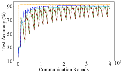
(b) $E=100$, $D=3$

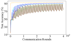
(c) $E=100$, $D=5$

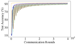
(d) $E=50$, $D=1$

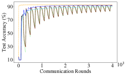
(e) $E=100$, $D=1$

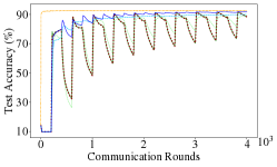
(f) $E=200$, $D=1$

Figure 8. Test accuracies of FedSGD, FedAvg, FedProx, FedLaAvg, and sequential SGD in the MNIST image classification task with different client availability settings.

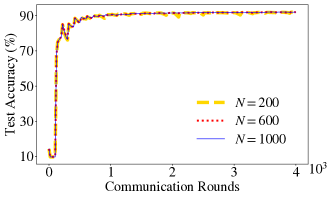
(a) Test accuracy with different $N$

(b) Test accuracy with different $\beta$

Figure 9. Test accuracies of FedLaAvg on MNIST dataset by varying the total number of clients $N$ and the proportion of selected clients $\beta$.

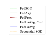
(a) Legends

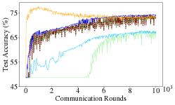
(b) $E=120$, $\alpha=0.25$

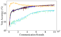
(c) $E=120$, $\alpha=0.5$

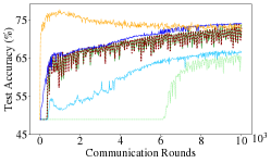
(d) $E=24$, $\alpha=0$

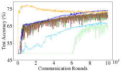
(e) $E=120$, $\alpha=0$

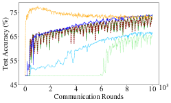
(f) $E=240$, $\alpha=0$

Figure 10. Test accuracies of FedSGD, FedAvg, FedProx, FedLaAvg, and sequential SGD in the Sentiment140 sentiment analysis task with different client availability settings.

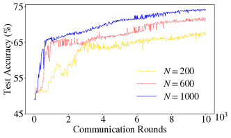
(a) Test accuracy with different $N$

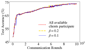
(b) Test accuracy with different $\beta$

Figure 11. Test accuracies of FedLaAvg on Sentiment140 dataset by varying the total number of clients $N$ and the proportion of selected clients $\beta$.

Appendix F Supplementary Notes for the Experiment Environment

The MNIST dataset is available from http://yann.lecun.com/exdb/mnist/. The Sentiment140 dataset is available from http://help.sentiment140.com/for-students. The pretrained GloVe embeddings can be downloaded from http://nlp.stanford.edu/data/glove.twitter.27B.zip. In addition, experiments are conducted on machines with operating system Ubuntu 18.04.3, CUDA version 10.1, and one NVIDIA GeForce RTX 2080Ti GPU. The average runtime on our machine is approximately 10 hours per experiment.

References

• (1)
• Bonawitz et al. (2019) Keith Bonawitz, Hubert Eichner, Wolfgang Grieskamp, Dzmitry Huba, Alex Ingerman, Vladimir Ivanov, Chloé Kiddon, Jakub Konečný, Stefano Mazzocchi, H. Brendan McMahan, Timon Van Overveldt, David Petrou, Daniel Ramage, and Jason Roselander. 2019. Towards Federated Learning at Scale: System Design. In Proceedings of MLSys.
• Cho et al. (2020) Yae Jee Cho, Jianyu Wang, and Gauri Joshi. 2020. Client Selection in Federated Learning: Convergence Analysis and Power-of-Choice Selection Strategies. CoRR abs/2010.01243 (2020).
• Eichner et al. (2019) Hubert Eichner, Tomer Koren, Brendan McMahan, Nathan Srebro, and Kunal Talwar. 2019. Semi-Cyclic Stochastic Gradient Descent. In Proceedings of ICML. 1764–1773.
• Go et al. (2009) Alec Go, Richa Bhayani, and Lei Huang. 2009. Twitter Sentiment Classification Using Distant Supervision. CS224N project report, Stanford (2009).
• Hard et al. (2018) Andrew Hard, Kanishka Rao, Rajiv Mathews, Françoise Beaufays, Sean Augenstein, Hubert Eichner, Chloé Kiddon, and Daniel Ramage. 2018. Federated Learning for Mobile Keyboard Prediction. CoRR abs/1811.03604 (2018).
• Hsieh et al. (2019) Kevin Hsieh, Amar Phanishayee, Onur Mutlu, and Phillip B. Gibbons. 2019. The Non-IID Data Quagmire of Decentralized Machine Learning. CoRR abs/1910.00189 (2019).
• Hu et al. (2020) Hanpeng Hu, Dan Wang, and Chuan Wu. 2020. Distributed Machine Learning through Heterogeneous Edge Systems. In Proceedings of AAAI. 7179–7186.
• Kairouz et al. (2019) Peter Kairouz, H. Brendan McMahan, Brendan Avent, Aurélien Bellet, Mehdi Bennis, Arjun Nitin Bhagoji, Keith Bonawitz, Zachary Charles, Graham Cormode, Rachel Cummings, Rafael G. L. D’Oliveira, Salim El Rouayheb, David Evans, Josh Gardner, Zachary Garrett, Adrià Gascón, Badih Ghazi, Phillip B. Gibbons, Marco Gruteser, Zaïd Harchaoui, Chaoyang He, Lie He, Zhouyuan Huo, Ben Hutchinson, Justin Hsu, Martin Jaggi, Tara Javidi, Gauri Joshi, Mikhail Khodak, Jakub Konecný, Aleksandra Korolova, Farinaz Koushanfar, Sanmi Koyejo, Tancrède Lepoint, Yang Liu, Prateek Mittal, Mehryar Mohri, Richard Nock, Ayfer Özgür, Rasmus Pagh, Mariana Raykova, Hang Qi, Daniel Ramage, Ramesh Raskar, Dawn Song, Weikang Song, Sebastian U. Stich, Ziteng Sun, Ananda Theertha Suresh, Florian Tramèr, Praneeth Vepakomma, Jianyu Wang, Li Xiong, Zheng Xu, Qiang Yang, Felix X. Yu, Han Yu, and Sen Zhao. 2019. Advances and Open Problems in Federated Learning. CoRR abs/1912.04977 (2019).
• Karimireddy et al. (2020) Sai Praneeth Karimireddy, Satyen Kale, Mehryar Mohri, Sashank J. Reddi, and Ananda Theertha Suresh. 2020. Scaffold: Stochastic Controlled Averaging for Federated Learning. In Proceedings of ICML.
• Khaled et al. (2019) Ahmed Khaled, Konstantin Mishchenko, and Peter Richtárik. 2019. First Analysis of Local GD on Heterogeneous Data. CoRR abs/1909.04715 (2019).
• LeCun et al. (1998) Yann LeCun, Léon Bottou, Yoshua Bengio, and Patrick Haffner. 1998. Gradient-Based Learning Applied to Document Recognition. Proc. IEEE (1998), 2278–2324.
• Li et al. (2019b) Liping Li, Wei Xu, Tianyi Chen, Georgios B. Giannakis, and Qing Ling. 2019b. RSA: Byzantine-Robust Stochastic Aggregation Methods for Distributed Learning from Heterogeneous Datasets. In Proceedings of AAAI. 1544–1551.
• Li et al. (2014) Mu Li, David G. Andersen, Jun Woo Park, Alexander J. Smola, Amr Ahmed, Vanja Josifovski, James Long, Eugene J. Shekita, and Bor-Yiing Su. 2014. Scaling Distributed Machine Learning with the Parameter Server. In Proceedings of OSDI. 583–598.
• Li et al. (2019a) Tian Li, Anit Kumar Sahu, Ameet Talwalkar, and Virginia Smith. 2019a. Federated Learning: Challenges, Methods, and Future Directions. CoRR abs/1908.07873 (2019).
• Li et al. (2020b) Tian Li, Anit Kumar Sahu, Manzil Zaheer, Maziar Sanjabi, Ameet Talwalkar, and Virginia Smith. 2020b. Federated Optimization in Heterogeneous Networks. In Proceedings of MLSys.
• Li et al. (2020a) Xiang Li, Kaixuan Huang, Wenhao Yang, Shusen Wang, and Zhihua Zhang. 2020a. On the Convergence of FedAvg on Non-IID Data. In Proceedings of ICLR.
• McMahan et al. (2017) Brendan McMahan, Eider Moore, Daniel Ramage, Seth Hampson, and Blaise Aguera y Arcas. 2017. Communication-Efficient Learning of Deep Networks from Decentralized Data. In Proceedings of AISTATS. 1273–1282.
• Mohri et al. (2019) Mehryar Mohri, Gary Sivek, and Ananda Theertha Suresh. 2019. Agnostic Federated Learning. In Proceedings of ICML. 4615–4625.
• Moreno-Torres et al. (2012) Jose G. Moreno-Torres, Troy Raeder, Rocío Alaiz-Rodríguez, Nitesh V. Chawla, and Francisco Herrera. 2012. A Unifying View on Dataset Shift in Classification. Pattern Recognition 45, 1 (2012), 521–530.
• Pennington et al. (2014) Jeffrey Pennington, Richard Socher, and Christopher D. Manning. 2014. Glove: Global Vectors for Word Representation. In Proceedings of EMNLP. 1532–1543.
• Quiñonero-Candela et al. (2009) Joaquin Quiñonero-Candela, Masashi Sugiyama Sugiyama, Anton Schwaighofer, and Neil D. Lawrence. 2009. Dataset Shift in Machine Learning. The MIT Press.
• Ruan et al. (2020) Yichen Ruan, Xiaoxi Zhang, Shu-Che Liang, and Carlee Joe-Wong. 2020. Towards Flexible Device Participation in Federated Learning for Non-IID Data. CoRR abs/2006.06954 (2020).
• Snoek et al. (2019) Jasper Snoek, Yaniv Ovadia, Emily Fertig, Balaji Lakshminarayanan, Sebastian Nowozin, D. Sculley, Joshua Dillon, Jie Ren, and Zachary Nado. 2019. Can You Trust Your Model’s Uncertainty? Evaluating Predictive Uncertainty under Dataset Shift. In Proceedings of NeurIPS. 13969–13980.
• Stich (2019) Sebastian U. Stich. 2019. Local SGD Converges Fast and Communicates Little. In Proceedings of ICLR.
• Stich et al. (2018) Sebastian U Stich, Jean-Baptiste Cordonnier, and Martin Jaggi. 2018. Sparsified SGD with Memory. In Proceedings of NeurIPS. 4447–4458.
• Stich and Karimireddy (2019) Sebastian U. Stich and Sai Praneeth Karimireddy. 2019. The Error-Feedback Framework: Better Rates for SGD with Delayed Gradients and Compressed Communication. CoRR abs/1909.05350 (2019).
• Subbaswamy et al. (2019) Adarsh Subbaswamy, Peter Schulam, and Suchi Saria. 2019. Preventing Failures Due to Dataset Shift: Learning Predictive Models That Transport. In Proceedings of AISTATS. 3118–3127.
• Tu et al. (2020) Yuwei Tu, Yichen Ruan, Satyavrat Wagle, Christopher G. Brinton, and Carlee Joe-Wong. 2020. Network-Aware Optimization of Distributed Learning for Fog Computing. In Proceedings of INFOCOM. 2509–2518.
• Wang and Joshi (2018) Jianyu Wang and Gauri Joshi. 2018. Cooperative SGD: A unified Framework for the Design and Analysis of Communication-Efficient SGD Algorithms. CoRR abs/1808.07576 (2018).
• Wang et al. (2020) Jianyu Wang, Qinghua Liu, Hao Liang, Gauri Joshi, and H. Vincent Poor. 2020. Tackling the Objective Inconsistency Problem in Heterogeneous Federated Optimization. In Proceedings of NeurIPS.
• Wu et al. (2020) Zhaoxian Wu, Qing Ling, Tianyi Chen, and Georgios B. Giannakis. 2020. Federated Variance-Reduced Stochastic Gradient Descent With Robustness to Byzantine Attacks. IEEE Trans. Signal Process. 68 (2020), 4583–4596.
• Yan et al. (2020) Yikai Yan, Chaoyue Niu, Yucheng Ding, Zhenzhe Zheng, Fan Wu, Guihai Chen, Shaojie Tang, and Zhihua Wu. 2020. Distributed Non-Convex Optimization with Sublinear Speedup under Intermittent Client Availability. CoRR abs/2002.07399 (2020).
• Yang et al. (2018) Timothy Yang, Galen Andrew, Hubert Eichner, Haicheng Sun, Wei Li, Nicholas Kong, Daniel Ramage, and Françoise Beaufays. 2018. Applied Federated Learning: Improving Google Keyboard Query Suggestions. CoRR abs/1812.02903 (2018).
• Yu et al. (2019a) Hao Yu, Rong Jin, and Sen Yang. 2019a. On the Linear Speedup Analysis of Communication Efficient Momentum SGD for Distributed Non-Convex Optimization. In Proceedings of ICML. 7184–7193.
• Yu et al. (2019b) Hao Yu, Sen Yang, and Shenghuo Zhu. 2019b. Parallel Restarted SGD with Faster Convergence and Less Communication: Demystifying Why Model Averaging Works for Deep Learning. In Proceedings of AAAI. 5693–5700.
• Zhang et al. (2012) Yuchen Zhang, Martin J Wainwright, and John C Duchi. 2012. Communication-Efficient Algorithms for Statistical Optimization. In Proceedings of NeurIPS. 1502–1510.