ResiliNet: Failure-Resilient Inference in Distributed Neural Networks

Abstract

Federated Learning aims to train distributed deep models without sharing the raw data with the centralized server. Similarly, in distributed inference of neural networks, by partitioning the network and distributing it across several physical nodes, activations and gradients are exchanged between physical nodes, rather than raw data. Nevertheless, when a neural network is partitioned and distributed among physical nodes, failure of physical nodes causes the failure of the neural units that are placed on those nodes, which results in a significant performance drop. Current approaches focus on resiliency of training in distributed neural networks. However, resiliency of inference in distributed neural networks is less explored. We introduce ResiliNet, a scheme for making inference in distributed neural networks resilient to physical node failures. ResiliNet combines two concepts to provide resiliency: skip hyperconnection, a concept for skipping nodes in distributed neural networks similar to skip connection in resnets, and a novel technique called failout, which is introduced in this paper. Failout simulates physical node failure conditions during training using dropout, and is specifically designed to improve the resiliency of distributed neural networks. The results of the experiments and ablation studies using three datasets confirm the ability of ResiliNet to provide inference resiliency for distributed neural networks.

1 Introduction

Deep neural networks (DNNs) have boosted the state-of-the-art performance in various domains, such as image classification, segmentation, natural language processing, and speech recognition (Krizhevsky et al., 2012; Hinton et al., 2012; LeCun et al., 2015; Sutskever et al., 2014). In certain DNN-empowered IoT applications, such as image-based defect detection or recognition of parts during product assembly, or anomaly behavior detection in a crowd, the inference task is intended to run for a prolonged period of time, that is, there is a continuous stream of samples in inference. In these applications, a recent trend (Teerapittayanon et al., 2017; Tao and Li, 2018) has been to partition and distribute the computation graph of a previously-trained neural network over physical nodes along an edge-to-cloud path (e.g. on edge and fog servers) so that the forward-propagation occurs in-network while the data traverses toward the cloud. This inference in distributed DNN architecture is motivated by two observations: Firstly, deploying DNNs directly onto IoT devices for huge multiply-add operations is often infeasible, as many IoT devices are low-powered and resource-constrained (Zhou et al., 2019a). Secondly, placing the DNNs in the cloud may not be reasonable for such prolonged inference tasks, as the raw data, which is often large, has to be continuously transmitted from IoT devices to the DNN model in the cloud, which results in the high consumption of network resources and possible privacy concerns (Jeong et al., 2018; Teerapittayanon et al., 2017).

A natural question that arises within this setting is whether the inference task of a distributed DNN is resilient to the failure of individual physical nodes, since distributing a DNN over several machines induces a higher risk of failures. The failure model in this paper is crash-only non-Byzantine; physical nodes could fail due to power outages, cable cuts, natural disasters, or hardware/software failures. Providing failure-resiliency for such inference tasks is vital, as physical node failures are more probable during a long-running inference task (e.g., in a continuous stream of samples). Failure of a physical node causes the failure of the DNN units that are placed on the node, and is especially troublesome for IoT applications that cannot tolerate poor performance while the physical node is being recovered. The following question is the topic of our study.

How can we make distributed DNN inference resilient to physical node failures?

Several frameworks have been developed for distributed training of neural networks (Abadi et al., 2016; Paszke et al., 2019; Chilimbi et al., 2014). On the other hand, inference in distributed DNNs has emerged as an approach for DNN-empowered IoT applications. Providing failure-resiliency during inference for such IoT applications is crucial. Authors in (Yousefpour et al., 2019) introduce the concept of skip hyperconnections in distributed DNNs that provides some failure-resiliency for inference in distributed DNNs. Skip hyperconnections skip one or more physical nodes in the vertical hierarchy of a distributed DNN. These forward connections between non-subsequent physical nodes help in making distributed DNNs more resilient to physical failures, as they provide alternative pathways for information when a physical node has failed. Although superficially they might seem similar to skip connections in residual networks (He et al., 2016a), skip hyperconnections serve a completely different purpose. While the former aim at solving the vanishing gradient problem during training, the latter are based on the underlying insight that during inference, if at least a part of the incoming information for a physical node is present (via skip hyperconnections), given their generalization power, the neural network may be able to provide a reasonable output, thus providing failure-resiliency.

A key observation in the aforementioned work is that the weights learned during training using skip hyperconnections are not aware that there might be physical node failures. In other words, the information about failure of physical nodes is not used during training to make the learned weights aware of such failures. As such, skip hyperconnections by themselves do not make the learned weights more resilient to physical failures, as they are just a way to diminish the effects of losing the information flow at inference time.

Key Contributions: Motivated by this limitation, (1) we introduce ResiliNet, which utilizes a new regularization scheme we call failout, in addition to skip hyperconnections, for making inference in distributed DNNs resilient to physical node failures. Failout is a regularization technique that during training “fails” (i.e. shuts down) the physical nodes of the distributed DNN, each hosting several neural network layers, thus simulating inference failure conditions. Failout effectively embeds a resiliency mechanism into the learned weights of the DNN, as it forces the use of skip hyperconnections during failure. The training procedure using failout could be applied offline, and would not necessarily be done during runtime (hence, shutting down physical nodes would be doing so in simulation). Although in DFG framework (Yousefpour et al., 2019) skip hyperconnections are always active both during training and inference, in ResiliNet skip hyperconnections are active during training and during inference only when the physical node that they bypass fails (for bandwidth savings).

(2) Through experiments using three datasets we show that ResiliNet minimizes the degradation impact of physical node failures during inference, under several failure conditions and network structures. Finally, (3) through extensive ablation studies, we explore the rate of failout, the weight of hyperconnections, and the sensitivity of skip hyperconnections in distributed DNNs. ResiliNet’s major novelty is in providing failure-resiliency through special training procedures, rather than traditional “system-based” approaches of redundancy, such as physical node replication or backup.

2 Resiliency-based Regularization for DNNs

2.1 Distributed neural networks

A distributed DNN is a DNN that is split according to a partition map and distributed over a set of physical nodes (a form of model parallelism). This concept is sometimes referred to as split learning, where only activations and gradients are transferred in the distributed DNN, which can result in improvements in privacy. This article studies the resiliency of previously-partitioned distributed DNN models during inference. We do not study the problem of optimal partitioning of a DNN; the optimal DNN partitioning depends on factors such as available network bandwidth, type of DNN layers, and the neural network topology (Hu et al., 2019; Kang et al., 2017; Zhou et al., 2019b). We do not consider doing any neural architecture search in this article. Nevertheless, in our experiments, we consider different partitions of the DNNs.

Since a distributed DNN resides on different physical nodes, during inference, the vector of output values from one physical node must be transferred (e.g. through a TCP socket) to another physical node. The transfer link (pipe) between two physical nodes is called a hyperconnection (Yousefpour et al., 2019). Hyperconnections transfer information (e.g. feature maps) as in traditional connections between neural network layers, but through a physical communication network. Unlike a typical neural network connection that connects two units and transfers a scalar, a hyperconnection connects two physical nodes and transfers a vector of scalars. Hyperconnections are one of two types: simple or skip. A simple hyperconnection connects a physical node to the physical node that has the next DNN layer. Skip hyperconnections are explained next.

2.2 Skip Hyperconnections

The concept of skip hyperconnections is similar to that of skip connections in residual networks (ResNets) (He et al., 2016a). A skip hyperconnection (Yousefpour et al., 2019) is a hyperconnection that skips one or more physical nodes in a distributed neural network, forwarding the information to a physical node that is further away in the distributed neural network structure. During training, the DNN learns to use the skip hyperconnections to allow a downstream physical node (closer to cloud) receive information from more than one upstream physical node. Consequently, during inference, if a physical node fails, information from the prior working nodes are still capable of propagating forward to downstream working physical nodes via these skip hyperconnections, providing some failure-resiliency (Yousefpour et al., 2019).

ResiliNet also uses skip hyperconnections, but in a slightly different manner from the DFG framework. When there is no failure during inference, or no failout during training (failout, to be discussed), the skip hyperconnections are not active. When failure occurs during inference (failures can be detected by simple heartbeat mechanisms), or failout during training, skip hyperconnections become active, to route the blocked information flow. This setup in ResiliNet significantly saves bandwidth, compared to DFG, which requires skip hyperconnections to be always active. The advantage here is in routing information during failure, that is otherwise not possible. Also, the bandwidth for the routed information over the failed node is the same as when there is no failure (skip hyperconnection only finds a detour). In the experiment we also show through experiments that if skip hyperconnections are always active, the performance only increases negligibly.

2.3 Failout Regularization

In the DFG framework (Yousefpour et al., 2019), the information regarding failure of the physical nodes is not used during training to make the learned weights more aware of such failures. Although skip hyperconnections increase the failure-resiliency of distributed DNNs, they do not make the learned weights more prepared for such failures. This is because all neural network components are present during training, as opposed to inference time where some physical nodes may fail. In order to account for the learned weights being more adapted to specific failure scenarios, we introduce failout regularization, which simulates inference-time physical node failure conditions during training.

During training, failout “fails” (i.e., shuts down) a physical node, to make the learned weights more adaptive to such failures and the distributed neural network more failure-resilient. By “failing” a physical node, we mean temporarily removing the neural network components that reside on the physical node, along with all their incoming and outgoing connections. Failout’s training procedure could be done offline, and would not necessarily be employed during runtime. Therefore failing physical nodes would be temporarily removing their neural network components in simulation.

When the neural components of a given physical node shut down using failout, the neural layers of the downstream physical node that are connected to the failing physical node will not receive information from the failing physical node, forcing their weights to take into account this situation and utilize the received information from the skip hyperconnection. In other words, failout forces the information passage through the skip hyperconnections during training, hence adapting the weights of the neural network to account for these failure scenarios during inference.

Formally, consider a neural network which is distributed over $V$ different nodes $v_{i}$, $i\in[1,V]$, where for each $v_{i}$, we define its failure rate (probability of failure) $f_{i}\in[0,1]$. Following this, we define a binary mask $b$ with $V$ components, where its $i$-th element $b_{i}$ follows a Bernoulli distribution, with a mean equal to $1-f_{i}$, that is $b_{i}\sim Ber(1-f_{i})$. During training, for each batch of examples, a new mask $b$ is sampled, and if $b_{i}=0$, the neural components of physical node $v_{i}$ are dropped from computation ($v_{i}$’s output is set to zero in simulated off-line training), thus simulating a real failure scenario. Formally, if $Y_{i}$ denotes the output of node $v_{i}$, then $Y_{i}=b_{i}H_{i}(X_{i})$, where $H_{i}(.)$ is a non-linear transform on $X_{i}$, the input of physical node $v_{i}$.

Consider a vertically distributed DNN where the nodes are numbered in sequence $1,2,\ldots,V$ from upstream to downstream (cloud). In this setting, for ResiliNet we can derive an equation for $X_{i+1}$, the input to node $v_{i}$, as

$$X_{i+1}=Y_{i}\odot Y_{i-1},$$ (1)

where the operator $\odot$ is defined as: in $X_{i+1}=Y_{i}\odot Y_{i-1}$, when node $v_{i}$ is alive $X_{i+1}=Y_{i}$, and when node $v_{i}$ fails, $X_{i+1}=Y_{i-1}$. In this definition, we can see that the skip hyperconnection is only active when there is a failure, which corresponds to ResiliNet. In the experiments, we also consider a case where skip hyperconnections are always active (we call it ResiliNet+), for which Eq. 1 is modified to

$$X_{i+1}=Y_{i}\oplus Y_{i-1}.$$ (2)

Although, superficially, failout seems similar to dropout (Srivastava et al., 2014), failout removes a whole segment of neural components, including neurons and weights, for a different purpose of failure-resiliency of distributed DNNs (and not only regularizing the neural network). Another distinction between failout and dropout is in their behavior during inference. In dropout, at inference, the weights of connections are multiplied by the probability of survival of their source neuron to account for model averaging from exponentially many thinned models. Furthermore, DNN units are not dropped during inference in dropout, making the model averaging a necessity. In contrast, failout does not multiply weights of hyperconnections by the probability of survival, since, during inference, physical nodes may fail, though not necessarily at the same rate as during training. Said differently, failout does not use the model ensemble analogy as used in standard dropout, hence does not need the mixed results of the model ensembles. To verify our hypothesis, we conducted experiments using different datasets in a setting where the weights of hyperconnections are multiplied by the probability of survival of the physical nodes, and we observed a sheer reduction in performance.

3 Experiments

We compare ResiliNet’s performance with that of DFG (Yousefpour et al., 2019) and vanilla (distributed DNN with no skip hyperconnections and no failout).

3.1 Scenarios and Datasets

Vertically distributed MLP: This is the simplest scenario for a distributed DNN in which the MLP is split vertically across physical nodes shown in the left of Fig. 2.

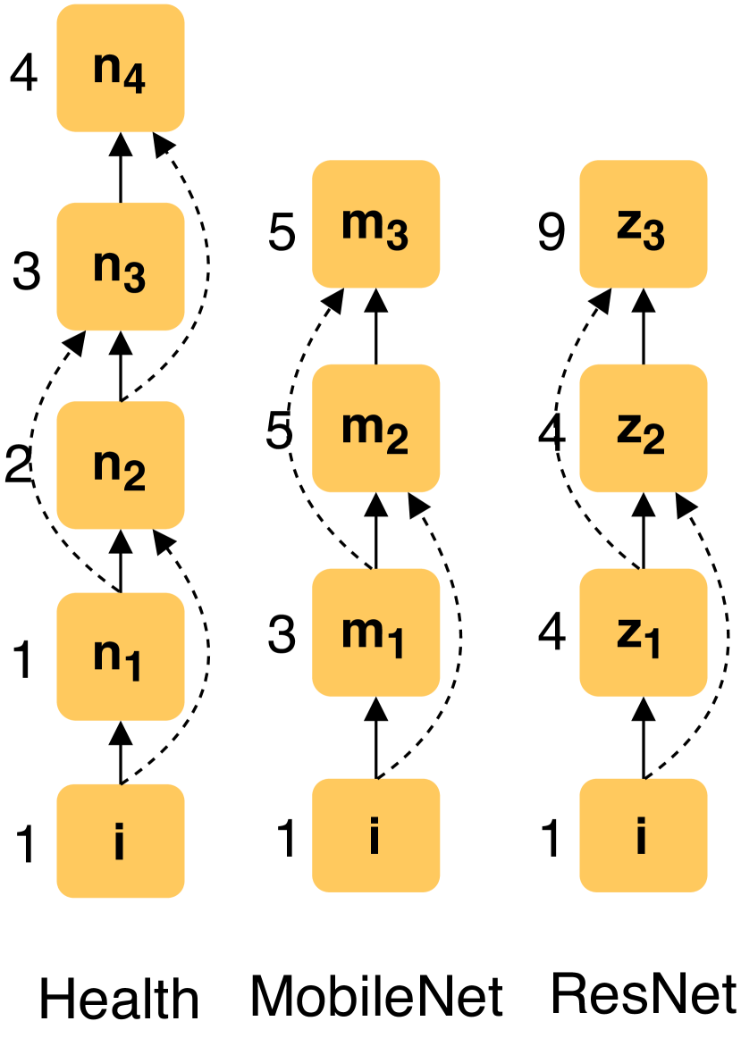
Figure 1: Distributed neural network setup and number of layers on each node.

Figure 2: Average performance

For this scenario, we use the UCI health activity classification dataset (“Health” for short), described in (Banos et al., 2015). This dataset is an example of an IoT application for medical purposes where the inference task will run over a long period of time. The dataset is comprised of readings from various sensors placed at the chest, left ankle, and right arm of 10 patients. There are a total of 23 features, each corresponding to a type of data collected from sensors. For this experiment, we split a DNN that consists of ten hidden layers of width 250, over 4 physical nodes as follows. The physical node $n_{1}$ hosts one hidden layer, $n_{2}$ two, $n_{3}$ three, and $n_{4}$ four (also summarized in Fig. 4). The dataset is labeled with the 12 activities a patient is performing at a given time, and the task is to classify the type of activity. We remove the activities that do not belong to one of the classes. After reprocessing, the dataset has 343,185 data points and is roughly uniformly distributed across each class. Hence, we use a standard cross-entropy loss function for the classification. For evaluation, we separate data into train, validation, and test with an 80/10/10 split.

Vertically distributed CNN: The two architectures in the right in Fig. 2 present the neural network structure proposed for these scenarios and how the CNNs are split. For these scenarios, we use two datasets, ImageNet Large Scale Visual Recognition Challenge (ILSVRC) and CIFAR-10. We utilize the ILSVRC dataset for measuring the performance of ResiliNet in distributed CNNs. However, for ablation studies for distributed CNNs, we use the CIFAR-10 dataset, since we run several iterations of experiments with different hyperparameters. We also employ data augmentation to improve model generalization.

For CIFAR-10 and ImageNet datasets, we use the MobileNetV1 CNN architecture  (Howard et al., 2017) and split it across 3 physical nodes. We chose version 1 of MobileNet (MobileNetV1), as it does not have any of the skip connections that are present in MobileNetV2. Moreover, since non-residual models cannot effectively deal with layer failure (Veit et al., 2016), we also consider neural networks with residual connections and experiment with ResNet-18 (He et al., 2016a). The ResNet-18 architecture has 18 layers, and we partition these stacked layers across the three physical nodes: $z_{1}$ contains four layers, $z_{2}$ four, and $z_{3}$ 9 plus the remaining layers. The MobileNetV1 architecture has 13 “stacked layers”, each with the following six layers: depth-wise convolution, batch normalization, ReLU, convolution, batch normalization, and ReLU. We partition these 13 stacked layers across the three physical nodes.

3.2 Experiment Settings

We implemented our experiments using TensorFlow and Keras on Amazon Web Service EC2 instances. Batch sizes of 1024, 128, and 1024 are used for the Health, CIFAR-10, and ImageNet experiments, respectively. The learning rate of 0.001 is used for the health activity classification and CIFAR-10 experiments. Learning rate decay with an initial rate of 0.01 is used for the ImageNet experiment. The image size of $160\times 160\times 3$ pixels is used for the ImageNet experiment. The rate of failout for ResiliNet is set to $10\%$ (other rates of failout are explored later in ablation studies).

Failure probabilities: To empirically evaluate different schemes, we use three different failure settings outlined in Fig. 4. A failure setting is a tuple, where each element $i$ is the probability that the physical node $v_{i}$ fails during inference. For example, the setting Normal could represent more reasonable network condition, where the probability of failure is low, while the settings Poor and Hazardous represent failure settings (only for experiments) when the failures are very frequent in the physical network. It is worth noting that the specific values of failure probabilities do not change the overall trend in the results and are only chosen so we have some benchmark for three different failure conditions.

To obtain values for the failure probabilities, we have the following observations: 1) the top physical node ($n_{4}$, $m_{3}$, $z_{3}$ in Fig. 2) is the cloud, and hence is always available; 2) the nodes closer to the cloud are more available than the ones far from the cloud; 3) the physical nodes closer to the cloud and data centers (e.g., backbone nodes) have relatively high availability of around 98% (Meza et al., 2018): such nodes have a mean time between failures (MTBF) of 3521 hours and a mean time to repair (MTTR) of 71 hours. Thus, the availability of those nodes is around 98%, while presumably the physical nodes closer to end-user are expected to have less availability, of around 92%-98% (in failure setting Normal). Once we obtain values for failure setting Normal, we simply increase them for settings Poor and Hazardous.

3.3 Performance Evaluation

	Failing		Top-1 Accuracy (%)
	Nodes	Prob. ($\%$)	ResiliNet+	ResiliNet	DFG	Vanilla
Health	None	87.43	97.85	97.77	97.90	97.85
	$n_{1}$	7.01	97.35	93.26	64.42	7.95
	$n_{2}$	3.64	94.32	95.59	22.49	7.99
	$n_{3}$	0.88	97.74	97.12	92.48	8.10
	$n_{1},n_{2}$	0.32	8.02	8.12	8.2	7.93
	$n_{1},n_{3}$	0.08	97.33	91.12	60.13	7.98
	$n_{2},n_{3}$	0.04	7.99	7.86	7.98	7.97
	$n_{1},n_{2},n_{3}$	0.003	7.98	8.11	7.89	7.91
	Average		97.36	97.02	92.21	86.57
MobileNet	None	94.08	88.11	87.75	87.54	86.64
	$m_{1}$	3.92	78.98	75.55	69.42	10.27
	$m_{2}$	1.92	75.65	59.18	62.76	9.85
	$m_{1},m_{2}$	0.08	9.71	10.11	10.02	10.07
	Average		87.45	86.66	86.29	82.1

Table 1: Individual physical node failures

Table 1 shows the performance of different schemes for certain physical node failures. The first two columns show the failing nodes, along with the probability of occurrence of those node failures under Normal failure setting. Recall that Vanilla is a distributed DNN that does not have skip hyperconnections and does not use failout. We assume that, when there is no information available to do the classification task due to failures, we do random guessing. ResiliNet+ is a scheme based on ResiliNet where skip hyperconnections are always active, during inference (or validation) and training. (In this table, for MobileNet experiment CIFAR-10 dataset is used).

Figure 3: Experiment settings

Experiment	Dist. MLP	Dist. MobileNet	Dist. ResNet-18
Dataset	UCI Health	ImageNet, CIFAR-10	CIFAR-10
Nodes Order	$[n_{4},n_{3},n_{2},n_{1}]$	$[m_{3},m_{2},m_{1}]$	$[z_{3},z_{2},z_{1}]$
Failure Setting
Normal	$[0\%,1\%,4\%,8\%]$	$[0\%,2\%,4\%]$	$[0\%,2\%,4\%]$
Poor	$[0\%,5\%,9\%,13\%]$	$[0\%,5\%,10\%]$	$[0\%,5\%,10\%]$
Hazardous	[$0\%,15\%,20\%,22\%]$	$[0\%,15\%,20\%]$	$[0\%,15\%,20\%]$

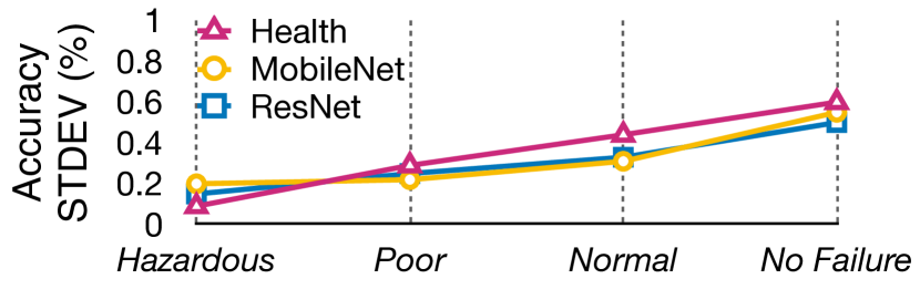
Figure 4: Impact of hypercon. weight in ResiliNet

(a) Health: In the health activity classification experiment, we see that the failure of even a single physical node compromises the performance of Vanilla due to random guessing, resulting top-1 accuracy of around 8%. On the other hand, DFG, ResiliNet, and ResiliNet+ subvert Vanilla’s inability to pass data over failed physical nodes, thereby achieving significantly greater performance. The results also show that, in this experiment, ResiliNet and ResiliNet+ perform better than DFG in all of the cases, except for when there is no failure. In certain physical nodes failures, such as when $n_{1}$, $n_{2}$, or $\{n_{1},n_{3}\}$ fail, ResiliNet and ResiliNet+ greatly surpass the accuracy of the both DFG and Vanilla, providing a high level of failure-resiliency. When physical node failures $\{n_{1},n_{2}\}$ and $\{n_{2},n_{3}\}$ occur, all schemes do not provide high accuracy, due to inaccessibility of the path for information flow.

(b) MobileNet on CIFAR-10: In the MobileNet experiment with CIFAR-10 dataset, Vanilla is outperformed by other three schemes when there is any combination of failures. ResiliNet and ResiliNet+ both offer a great performance when $m_{1}$ fails; nevertheless, DFG performs marginally better than ResiliNet when $m_{2}$ fails. ResiliNet+ consistently has the highest accuracy in this experiment.

We can see that ResiliNet overall maintains a higher accuracy than DFG and vanilla. We can also see that ResiliNet+ outperforms all of the schemes. However, this benefit comes at a cost of having the skip hyperconnections always active, which results in higher bandwidth usage. In the rest of the experiments, we choose ResiliNet among the two ResiliNets. This is a pessimistic choice and it is justified by the bandwidth savings.

Previously, we discussed and showed how the accuracy is affected when particular physical nodes fail. Nevertheless, some of the physical node failures are not as probable as others (e.g. multiple physical nodes failure vs. single physical node failure), and hence it is interesting to see the average accuracy in different node failure settings. Fig. 2 shows the average top-1 accuracy of the three methods under different failure settings, with 10 iterations for the health activity classification experiment, and 2 iterations for the MobileNet experiment on ImageNet (confidence intervals are very small and negligible and are omitted). Key result 1: as expected, in both experiments, ResiliNet seems to outperform DFG and Vanilla. The high performance of ResiliNet is more evident in severe node failure conditions.

3.4 Ablation Studies

Now that the validity of failout has been empirically shown to provide an increase in failure-resiliency of distributed neural networks, we now investigate the importance of individual skip hyperconnections, their weights, as well as the optimal rate of failout. To do so, we raise four important questions in what follows and empirically provide answers to these questions. We use the CIFAR-10 dataset for ablation studies of the distributed CNN, and use Health for ablation studies of distributed MLPs.

1. What is the best choice of weights for the hyperconnections? Hyperconnections can have weights, similar to the weights of the connections in neural networks. We begin by assessing the choice of weights of the hyperconnections. Although by default, the weight of hyperconnections in ResiliNet is $\mathbf{1}$, we pondered if setting the weights relative to the reliability of their source physical nodes could improve the accuracy. Reliability of a physical node $v_{i}$ is $r_{i}=(1-p_{i})$, where $p_{i}$ is the probability of failure of node $v_{i}$. We proposed two heuristics, called “Relative Reliability” and “Reliability,” that are described as follows:
Consider two physical nodes $v_{1}$ and $v_{2}$ feeding data through hyperconnections to physical node $v_{3}$. If physical node $v_{1}$ is less reliable than physical node $v_{2}$ ($r_{1}<r_{2}$), setting $v_{1}$’s hyperconnections weight with a smaller value than that of $v_{2}$ may improve the performance. Thus, for the hyperconnection weight connecting node $v_{i}$ to node $v_{j}$, in Reliability heuristic, we set $\mathbf{\overline{\overline{w}}}_{ij}=r_{i}$, where $\mathbf{\overline{\overline{w}}}_{ij}$ denotes the weight of hyperconnection from physical node $v_{i}$ to node $v_{j}$. Comparably, in Relative Reliability heuristic, we set $\mathbf{\overline{\overline{w}}}_{ij}=\frac{r_{i}}{\sum_{k\in H_{j}}{r_{k}}}$, where $H_{j}$ is the set of incoming hyperconnection indices to the physical node $v_{j}$.

We experiment with the following four hyperconnection weight schemes in ResiliNet for 10 runs: (1) weight of $\mathbf{1}$, (2) Reliability heuristic, (3) Relative Reliability heuristic, and (4) uniform random weight between 0 and 1. Key result 2: surprisingly, all of the four hyperconnection weight schemes resulted in a similar performance. Since all of the values for average accuracy are similar in these experiments, we report in Fig. 4 the standard deviation among these weight schemes in ResiliNet.

We see that the standard deviation among the weight schemes is negligible, constantly below 1%. This suggests that there may not be a significant difference in accuracy when using any of the reasonable weighting scheme (e.g. heuristic of $\mathbf{1}$). Key observation 1: we also experimented with a scheme in which the hyperconnection weight is uniformly and randomly distributed between 0 and 10, and observed that the accuracy dropped significantly for the distributed MLPs. Key observation 2: surprisingly, the accuracy of distributed CNNs stays in the same range as in other schemes, when hyperconnection weight is a uniform random number between 0 and 10. We hypothesize that, for distributed MLPs, a reasonable hyperconnection weight scheme is a scheme that assigns the weights of hyperconnections between 0 and 1. Nevertheless, further investigation may be required in different distributed DNN architectures to assess the full effectiveness of hyperconnection weights.

Table 2: Impact of failout rate in ResiliNet. Numbers represent average top-1 accuracy in %.

Failout Rate	“Failure”			5%			10%			30%			50%
Experiment	H	M	R	H	M	R	H	M	R	H	M	R	H	M	R
Failure Setting
No Failure	N/A	N/A	N/A	97.84	88.23	91.94	97.81	88.53	91.43	97.53	87.75	88.44	96.92	84.60	85.79
Normal	96.32	86.78	89.54	96.64	85.03	89.50	97.07	85.87	88.70	97.04	86.66	86.28	96.52	84.01	84.13
Poor	95.81	81.61	86.16	94.96	80.30	85.81	95.70	81.92	84.59	95.86	84.92	82.97	95.38	82.99	81.55
Hazardous	91.95	77.46	78.60	89.36	70.32	78.82	90.58	73.16	77.03	91.06	79.93	76.97	90.67	79.35	76.65

2. What is the optimal rate of failout? In this ablation experiment, we investigate the effect of failout by setting the rate of failout to fixed rates of 5%, 10%, 30%, 50%, and a varying rate of “Failure,” where the failout rate for a physical node is equal to its probability of failure during inference. Table 2 illustrates the impact of failout rate in ResiliNet. Key result 3: ResNet (R) seems to favor Failure failout rate, and MobileNet (M) favors higher failout rates of around 30%.. Key observation 3: we hypothesize that, since a significant portion of the DNN is dropped during training when using failout, higher failout rate results in lower accuracy, as opposed to standard dropout. Key observation 4: based on our preliminary experiments, we conclude that the optimal failout rate should be seen as a hyperparameter, and be tuned for the experiment.

3. Which skip hyperconnections are more important? It is important to see which skip hyperconnections in ResiliNet are more important, thereby contributing more to the resiliency of the distributed neural network. This is helpful for certain scenarios in which having all skip hyperconnections is not possible (e.g. due to the cost of establishing new connections, or some communication constraints). To perform these experiments, we shut down (i.e. disconnect) a certain configuration of skip hyperconnections while keeping other skip hyperconnections active and every experiment setting the same, to see changes in the performance. The results are presented in Fig. 5. The bars show the average top-1 accuracy of 10 runs, under different “configs” in which a certain combination of skip hyperconnections are shut down. The present skip hyperconnections are shown in the tables next to the bar charts. Letters in the tables indicate the source physical node of the skip hyperconnection. In the health activity classification experiment, since there are three skip hyperconnections in the distributed neural network, there are eight possible configurations of skip hyperconnections (“Config 1” through “Config 8”). Similarly, in the experiments with MobileNet and ResNet-18, we consider all four configurations, as we have two skip hyperconnections.

In the health activity classification (Fig. 5a), we can see a uniform accuracy gain, when going from Config 1 towards Config 8. We can also see that, by looking at Config 2 through Config 4, if only one skip hyperconnection is allowed in a scenario, it should be the skip hyperconnection from input to $n_{2}$ (labeled as $i$). This is also evident when comparing Config 5 and Config 6: the skip hyperconnection from input to $n_{2}$ is more important. In the Hazardous reliability scenario, a proper subset of two skip hyperconnections can achieve up to a 24% increase in average accuracy (Config 1 vs. Config 6). Key result 4: this hints that individual skip hyperconnections are more important when there are more failures in the network. In the experiment with MobileNet, we also observe a uniform accuracy increase, when going from Config 1 towards Config 4. We can see that the skip hyperconnection from input to $m_{2}$ is more important that the skip hyperconnection from $m_{1}$ to $m_{3}$ (Config 2 vs. Config 3). Nonetheless, if both skip hyperconnections are present (Config 4), the performance is at its peak. Comparably, in the experiment with ResNet (Fig. 5c), we can see that the skip hyperconnection from node $z_{1}$ to $z_{3}$ is more important than the skip hyperconnection from input to $z_{2}$. We can also see that, when we have all the skip hyperconnections, the performance of the distributed DNNs are at their peak.

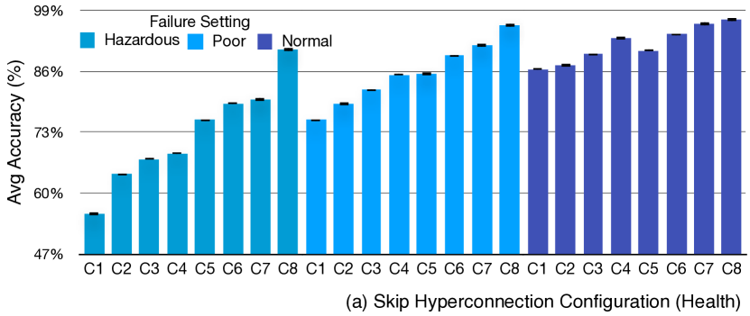
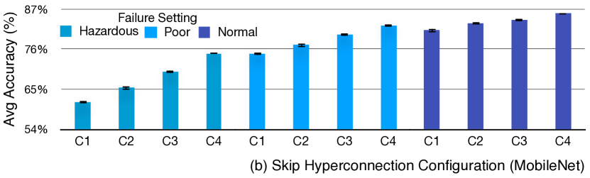
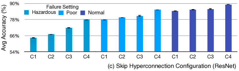
Config	Skip Hyperconnection
C1	None
C2	$n$ 2
C3	$n$ 1
C4	$i$
C5	$n$ 1 , $n$ 2
C6	$n$ 2 , $i$
C7	$n$ 1 , $i$
C8	All
Config	Skip Hyperconnection
C1	None
C2	$m$ 1
C3	$i$
C4	All
Config	Skip Hyperconnection
C1	None
C2	$i$
C3	$z$ 1
C4	All

Figure 5: Ablation studies for analyzing sensitivity of ResiliNet’s skip hyperconnections in (a) health activity classification experiment, (b) MobileNet experiment, (c) ResNet experiment. The charts show average top-1 accuracy (with error bars showing standard deviation). The tables to the right of the charts show the present skip hyperconnections in each skip hyperconnection configuration. (Notation: letters indicate the source physical node of the corresponding skip hyperconnection)

This ablation study demonstrates that, by searching for a particular important subset of skip hyperconnections in a distributed neural network, especially in the Hazardous reliability scenarios, we can achieve a large increase in the average accuracy. We point the interested reader to (He et al., 2016b; Veit et al., 2016; Jastrzebski et al., 2018) for more in-depth analyses of representations and functions induced by skip connections in neural networks.

4 Related Work

a. Distributed Neural Networks. Federated Learning is a paradigm that allows clients collaboratively train a shared global model (Wang et al., 2020; Kairouz et al., 2019; Bonawitz et al., 2019). Similarly, distributed training of neural networks has received significant attention (Abadi et al., 2016; Paszke et al., 2019; Chilimbi et al., 2014). Resilient distributed training against adversaries is studied in  (Chen et al., 2018; Damaskinos et al., 2019). Nevertheless, inference in distributed neural networks is less explored, although application scenarios that need ongoing and long inference tasks are emerging (Teerapittayanon et al., 2017; Morshed et al., 2017; Liu et al., 2018; Tao and Li, 2018; Hu et al., 2019; Dey et al., 2019).

b. Neural Network Fault Tolerance. A related concept to failure is fault, which is when units or weights become defective (i.e. stuck at a certain value, or random bit flip). Studies on fault tolerance of neural networks date back to the early 90s, and are limited to mathematical models of small neural networks (e.g. neural networks with one hidden layer or unit-only and weight-only faults) (Mehrotra et al., 1994; Bolt, 1992; Phatak and Koren, 1995).

c. Neural Network Robustness. A line of research related to our study is robust neural networks (Goodfellow et al., 2015; Szegedy et al., 2014; Cisse et al., 2017; Bastani et al., 2016; El Mhamdi et al., 2017). Robustness in neural networks has gained considerable attention lately, and is especially important when the neural networks are to be developed in commercial products. These studies are primarily focused on adversarial examples, examples that are only slightly different from correctly classified examples drawn from the data distribution. Despite the relation to our study, we are not focusing on the robustness of neural networks to adversarial examples. We study resiliency of distributed DNN inference in the presence of failure of a large group of neural network units. DFG framework in (Yousefpour et al., 2019) uses skip hyperconnections for failure-resiliency of distributed DNN inference. We showed how ResiliNet differs from DFG in skip hyperconnections setup, and in its novel use of failout to provide greater failure-resiliency.

d. Regularization Methods. Some regularization methods that implicitly increase robustness are dropout (Srivastava et al., 2014), dropConnect (Wan et al., 2013), DropBlock (Ghiasi et al., 2018), zoneout (Krueger et al., 2016), cutout (DeVries and Taylor, 2017), swapout (Singh et al., 2016), and stochastic depth (Huang et al., 2016). Although there are similarities between failout and these methods in terms of the regularization procedure, these methods largely differ in spirit from ours. In particular, although during training, dropout turns off neurons and dropConnect discards weights, they both enable an ensemble of models for regularization. On the other hand, failout shuts down an entire physical node in a distributed neural network to simulate actual failures in the physical network, for providing failure-resiliency. Stochastic depth is a procedure to train very deep neural networks effectively and efficiently. The focus of zoneout, DropBlock, swapout, and cutout is on regularizing recurrent neural networks and CNNs, while they are not designed for failure-resiliency.

5 Conclusion

Federated Learning utilize deep learning models for training or inference without accessing raw data from clients. Similarly, we presented ResiliNet, a framework for providing failure-resiliency of distributed DNN inference that combines two concepts: skip hyperconnections and failout. We saw how ResiliNet can improve the failure-resiliency of distributed MLPs and distributed CNNs. We also observed experimentally that, the weight of hyperconnections may not change the performance of distributed DNNs if the hyperconnections weights are chosen in certain range. We also observed that the rate of failout should be seen as a hyperparameter and be tuned. Finally, we observed that some skip hyperconnections are more important than others, especially under more extreme failure scenarios.

Future Work: We view ResiliNet as an important first step in studying failure-resiliency in distributed DNNs. This study opens several paths for related research opportunities. Firstly, it is interesting to study the distributed DNNs that are both horizontally and vertically distributed. Moreover, finding optimal hyperconnection weights through training (not through heuristics) may be a future research direction. Finally, instead of having only skip hyperconnection to bypass a node, we can have a skip layer, a layer to approximate the neural components of a failed physical node.

6 Broader and Ethical Impact

Energy and Resources: ResiliNet may take longer to converge, due to its failout regularization procedure. Moreover, if a distributed DNN is already trained, it needs to be re-trained with skip hyperconnections and failout; though, the training can be done offline. Additionally, some hyper-parameter tuning may be needed during training. These training settings depend on the availability of large computational resources that necessitate similarly substantial energy consumption (Strubell et al., 2019). We did not prioritize computationally efficient hardware and algorithms in the experiment. Nevertheless, if ResiliNet is deployed and is powered by renewable energy and, the impacts of the hyperparameter tuning will be offset over a long period of time. Regarding bandwidth usage, ResiliNet+ also increases the use of bandwidth due the activity of the skip hyperconnections both during training and inference.

Bias: Secondly, as the large scale deployment of powerful deep learning algorithms becomes easier and more practical, the number of new applications that will use the infrastructure will undoubtedly grow. With the new applications, there is a risk that models are over-fit and biased to a particular setting. The bias and over-fit may impact people (e.g. when the model may not be “fair”), especially when more people become users of such applications. Although we do not provide solutions or countermeasures to these issues, we acknowledge that this type of research can implicitly carry a negative impact in the future regarding the issues described above. Follow-up work focusing on applications must therefore include this type of consideration.

7 Supplementary Material

7.1 Different configurations of hyperconnections

In this paper, all of the experiments are conducted on vertically distributed DNNs, as they are more common form of distributed DNNs. Nevertheless, one could imagine a distributed DNN that is both vertically and horizontally distributed. For example, when a DNN is used for image-based defect detection in a factory or automatic recognition of parts during product assembly, maybe it is distributed vertically and horizontally for dispersed presence (Teerapittayanon et al., 2017; Yousefpour et al., 2019). In these cases, the horizontal distribution of DNN helps to extend the DNN to multiple regions which may are geographically distributed. As an example, in a case where inference runs across geographically distributed sites, the first few layers of the distributed DNN can be duplicated (horizontally) and placed on the corresponding physical nodes in those sites, so that they can perform the forward pass on the first few layers. One (or more) downstream node can then combine the immediate activations sent from those physical nodes and send the combined activation to the upper layers of the DNN.

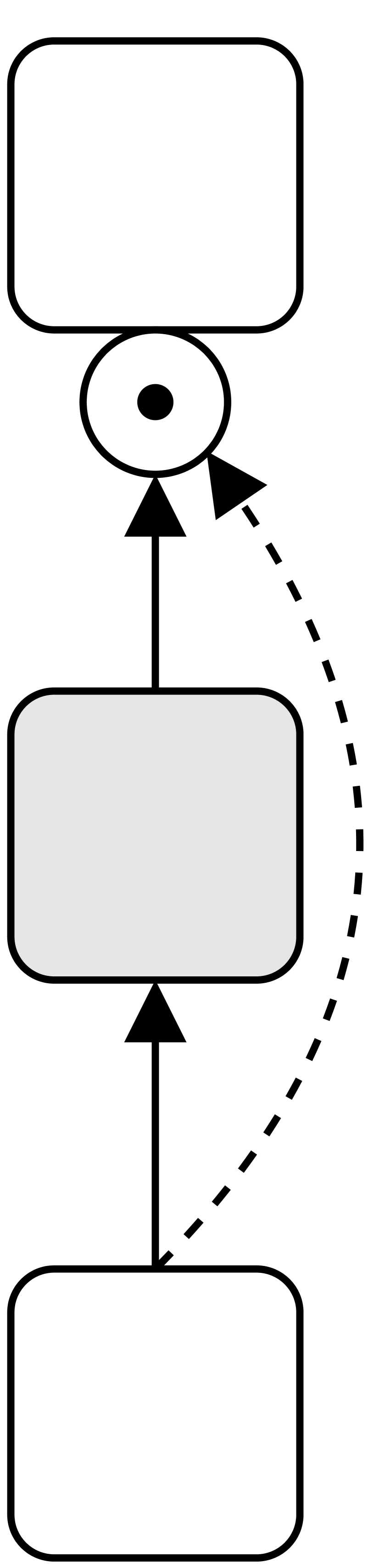
(a) b

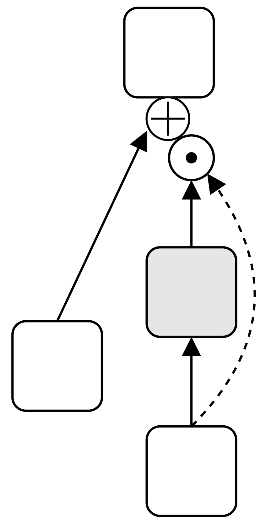
(b)

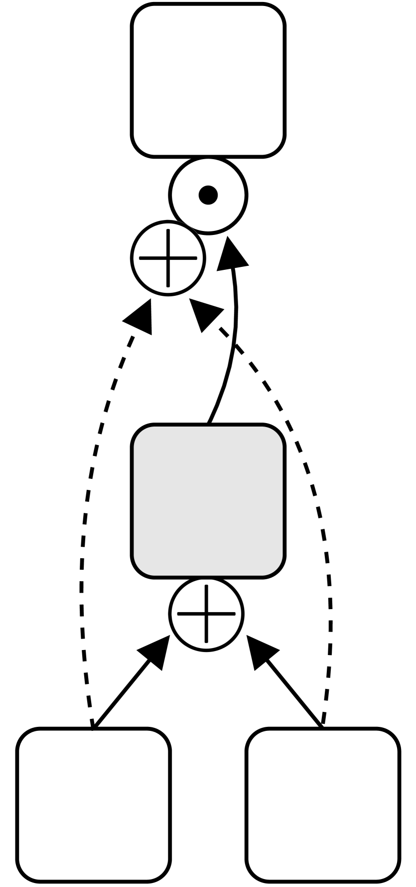
(c)

Figure 6: ResiliNet’s configurations of hyperconnections. Boxes denote physical nodes and arrows denote hyperconnections. The shaded physical node is the “failing node” that undergoes failure (during inference) or failout (during training). (a) The failing node is the only child of its parent and has only one child, (b) The failing node is not the only child of its parent and has one child, (c) The failing node is the only child of its parent and has more than one child.

Figure 6 shows ResiliNet’s different configurations of hyperconnections. Figure 6a shows a vertically distributed DNN, and Fig. 6b and Fig. 6c show a distributed DNN that is both vertically and horizontally distributed. Other distributed DNN architectures could be constructed based on the combination of these three basic hyperconnection configurations. In ResiliNet, skip hyperconnections are active only during failure or failout; Thus, in Fig. 6, the symbol $\odot$ represents this behavior, which was defined previously in the paper as follows: in $X_{i+1}=Y_{i}\odot Y_{i-1}$, when node $v_{i}$ (shaded in gray in Fig. 6a) is alive $X_{i+1}=Y_{i}$, and when node $v_{i}$ fails, $X_{i+1}=Y_{i-1}$. The symbol $\oplus$ simply denotes addition. For instance, in Fig. 6b, the input to the top node is the sum of the output of the node on the left, and the output of one of the nodes on the right, depending on if the gray node is alive or not. Recall that in ResiliNet+, we replace the symbol $\odot$ with the symbol $\oplus$. Thus, in the figure for hyperconnection configurations of ResiliNet+, we would just have a single symbol $\oplus$ on the input to the top node that adds all the incoming outputs.

7.2 Different Structure of distributed DNN

In this subsection, to verify our claims regarding the superior performance of ResiliNet, we consider different partitions of DNNs onto distributed physical nodes and measure their performance. For this ablation study, we consider the distributed MLP in health activity classification experiment, and the distributed MobileNet. For the MLP in health activity classification experiment, instead of the 1$\rightarrow$1$\rightarrow$2$\rightarrow$3$\rightarrow$4 partition that we considered in the paper, we experiment with partition 1$\rightarrow$2$\rightarrow$3$\rightarrow$2$\rightarrow$3. For MobileNet, instead of the 1$\rightarrow$3$\rightarrow$5$\rightarrow$5 partition, we experiment with partition 2$\rightarrow$2$\rightarrow$4$\rightarrow$6.

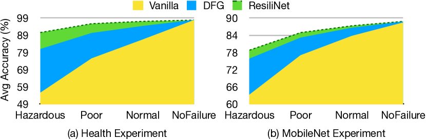
Figure 7: Average performance under new partition

The results of our experiments with these new two partitions are depicted in Fig. 7. We can see that, ResiliNet consistently outperforms both DFG and vanilla, and this verify our claims regarding the superior performance of ResiliNet in a new distributed DNN partition. We also experimented with other partitions, and observed the same trends.

8 Frequently Asked Questions

In this section, we hope to answer the frequently asked questions by the reviewers of this paper and the audience of this work when we present it.

8.1 What exactly the failure settings are and why nodes fail with those particular probabilities?

Answer: The failure settings are representations of real-world failure conditions, simply to show that under more severe conditions, ResiliNet’s benefit is more evident. And regarding failure values, the nodes closer to the cloud have less failure rate. That is why in Fig. 4 the failure rate of nodes closer to the cloud are less than those farther from the cloud. See the next question.

8.2 What is a typical failure probability in a real system?

Answer: For cloud, it is almost 0% (99.999% availability). Devices closer to the cloud and data centers, e.g., backbone nodes, have also relatively high availability; according to Meza, Justin, et al. “A large scale study of data center network reliability”, published in Proceedings of the Internet Measurement Conference, 90% of such nodes have a mean time between failures (MTBF) of 3521 hours and a mean time to repair (MTTR) of 71 hours. Thus, the availability of those nodes is around 98%. Devices closer to end-user are expected to have less availability, of around 92%-98%. These numbers are in accordance with the failure setting “Normal” in the paper. Similarly, other failure settings have lower reliability.

8.3 How does time to detect a failure impact ResiliNet in a real deployment?

Answer: Note that with the heartbeat mechanism (mentioned in the paper), time to detect a failure is in order of seconds (at most minutes), while the time to fix a node is in order of hours; per Meza, Justin, et al. “A large scale study of data center network reliability”, published in Proceedings of the Internet Measurement Conference, 90% of backbone nodes have a mean time to repair of 71 hours.

8.4 What is the failure model of physical nodes?

Answer: Our failure model is crash-only non-Byzantine.

8.5 Do skip hyperconnections increase bandwidth usage?

Answer: In ResiliNet, skip hyperconnections are active only during failure (and during failout), and they only route the blocked information flow. Note that skip hyperconnection’s advantage is in routing information during failure, that is otherwise not possible. The bandwidth for the routed information over the failed node is the same as when there is no failure (skip hyperconnection only finds a detour).

8.6 What is the bandwidth savings of ResiliNet?

Answer: Here we measure the bandwidth savings of ResiliNet compared to DFG. In DFG, skip hyperconnections are always active during training and inference. However, in ResiliNet, skip hyperconnections are only activated when a node fails. To obtain the bandwidth savings, we measure the size of the data that is passed among nodes at any given time. Table 3 shows the bandwidth savings in different experiments.

Table 3: Bandwidth savings of ResiliNet

Experiment	Dist. MLP	Dist. MobileNet	Dist. ResNet-18
Dataset	UCI Health	ImageNet     CIFAR-10	CIFAR-10
Bandwidth savings	$40.35\%$	$47.06\%$     $46.23\%$	$40.61\%$

8.7 How about experiments on actual sensors and devices?

Answer: The training procedure in ResiliNet can be performed completely off-line (not during runtime), and later the learned network can be deployed. Hence, the actual deployment would not impact the training. It is also worth noting that, with real implementation, since the failure rates and time to repair during inference are most larger, the benefits of ResiliNet would be more evident. Recall that the benefit of ResiliNet is more evident in more extreme failure conditions.

8.8 Is this distributed inference framework related to Federated Learning?

Answer: This is a similar setting to Federated Learning, but it differs from it significantly. Federated Learning aims to train distributed deep models without sharing the raw data with the centralized server. In Federated Learning, model parameters are available to all participants and data are locally distributed among devices. Conversely, in distributed inference of neural networks, model parameters are split by different nodes. In other words, by partitioning the network and distributing it across several physical nodes, activations and gradients are exchanged between physical nodes, rather than raw data.

8.9 Is there any assumption on the distribution of data on different nodes?

Answer: No, we do not assume any distribution of data (e.g. on IoT nodes).

8.10 What is the suggested/optimal range for failout rate?

Answer: Based on Table 2 the rate of failout should be chosen less than 0.5.

8.11 Why is failout related to regularization?

Answer: The main similarities can be drawn to dropout regularization, which serves as the main inspiration to this work. In dropout, by dropping units at random in layers of neural network, the learned weights are regularized to show a more robust behavior that does not depend entirely on output of one particular set of neurons, but on all of them as a whole. Similarly, in failout we randomly drop a physical node, which allows regularizing weights in the following nodes, making them less dependent on this particular node (which can fail).

8.12 How are skip hyperconnections activated? What is the protocol to reconfigure?

Answer: ResiliNet simply routes information through the skip hyperconnection, when a failure is detected. Once failed node is fixed, ResiliNet turns off the skip hyperconnection and sends the data normally.

8.13 Why not permit a systems approach of dynamically provisioning a replica to replace the faulty node?

Answer: We think this approach is not as efficient as simply starting a new connection upon failure of a node. In the systems approach, we would have some sort of a backup node or a reserved resource, to start upon failure; in ResiliNet we just open a connection (e.g., TCP connection) after failure detection for starting a skip hyperconnection.

8.14 How much do skip hyperconnections add to the size of the model and training time?

Answer: When hyperconnections do not normally introduce new parameters their size is negligible. Only when hyperconnections need to match the dimensions (e.g., in CNNs), they introduce new parameters. The training time is in fact slightly reduced, as training time is usually faster with networks with residual connection (skip hyperconnections are similar to residual connections).

References

- (1)
- Abadi et al. (2016) Martín Abadi, Paul Barham, Jianmin Chen, Zhifeng Chen, Andy Davis, Jeffrey Dean, Matthieu Devin, Sanjay Ghemawat, Geoffrey Irving, Michael Isard, et al. 2016. Tensorflow: a system for large-scale machine learning.. In OSDI, Vol. 16. 265–283.
- Banos et al. (2015) Oresti Banos, Claudia Villalonga, Rafael Garcia, Alejandro Saez, Miguel Damas, Juan A Holgado-Terriza, Sungyong Lee, Hector Pomares, and Ignacio Rojas. 2015. Design, implementation and validation of a novel open framework for agile development of mobile health applications. Biomedical engineering online 14, 2 (2015).
- Bastani et al. (2016) Osbert Bastani, Yani Ioannou, Leonidas Lampropoulos, Dimitrios Vytiniotis, Aditya Nori, and Antonio Criminisi. 2016. Measuring neural net robustness with constraints. In Neural Information Processing Systems (NeurIPS). 2613–2621.
- Bolt (1992) George Ravuama Bolt. 1992. Fault Tolerance in Artificial Neural Networks. Ph.D. Dissertation. University of York.
- Bonawitz et al. (2019) Keith Bonawitz, Hubert Eichner, Wolfgang Grieskamp, Dzmitry Huba, Alex Ingerman, Vladimir Ivanov, Chloe Kiddon, Jakub Konecny, Stefano Mazzocchi, H Brendan McMahan, et al. 2019. Towards federated learning at scale: System design. arXiv preprint arXiv:1902.01046 (2019).
- Chen et al. (2018) Lingjiao Chen, Hongyi Wang, Zachary Charles, and Dimitris Papailiopoulos. 2018. DRACO: Byzantine-resilient Distributed Training via Redundant Gradients. In Proceedings of the 35th International Conference on Machine Learning, Vol. 80. PMLR, 903–912.
- Chilimbi et al. (2014) Trishul M Chilimbi, Yutaka Suzue, Johnson Apacible, and Karthik Kalyanaraman. 2014. Project Adam: Building an Efficient and Scalable Deep Learning Training System.. In OSDI, Vol. 14. 571–582.
- Cisse et al. (2017) Moustapha Cisse, Piotr Bojanowski, Edouard Grave, Yann Dauphin, and Nicolas Usunier. 2017. Parseval networks: Improving robustness to adversarial examples. In Proceedings of the 34th International Conference on Machine Learning-Volume 70. JMLR, 854–863.
- Damaskinos et al. (2019) Georgios Damaskinos, El Mahdi El Mhamdi, Rachid Guerraoui, Arsany Hany Abdelmessih Guirguis, and Sébastien Louis Alexandre Rouault. 2019. AGGREGATHOR: Byzantine Machine Learning via Robust Gradient Aggregation. (2019). Conference on Systems and Machine Learning (SysML).
- DeVries and Taylor (2017) Terrance DeVries and Graham W Taylor. 2017. Improved Regularization of Convolutional Neural Networks with Cutout. arXiv preprint arXiv:1708.04552 (2017).
- Dey et al. (2019) Swarnava Dey, Jayeeta Mondal, and Arijit Mukherjee. 2019. Offloaded Execution of Deep Learning Inference at Edge: Challenges and Insights. In IEEE International Conference on Pervasive Computing and Communications Workshops. 855–861.
- El Mhamdi et al. (2017) EM El Mhamdi, R Guerraoui, and S Rouault. 2017. On the robustness of a neural network. In 2017 IEEE 36th Symposium on Reliable Distributed Systems (SRDS). 84–93.
- Ghiasi et al. (2018) Golnaz Ghiasi, Tsung-Yi Lin, and Quoc V Le. 2018. Dropblock: A regularization method for convolutional networks. In Advances in Neural Information Processing Systems. 10727–10737.
- Goodfellow et al. (2015) Ian Goodfellow, Jonathon Shlens, and Christian Szegedy. 2015. Explaining and Harnessing Adversarial Examples. In International Conference on Learning Representations.
- He et al. (2016a) Kaiming He, Xiangyu Zhang, Shaoqing Ren, and Jian Sun. 2016a. Deep residual learning for image recognition. In Proceedings of the IEEE conference on computer vision and pattern recognition (CVPR). 770–778.
- He et al. (2016b) Kaiming He, Xiangyu Zhang, Shaoqing Ren, and Jian Sun. 2016b. Identity mappings in deep residual networks. In European conference on computer vision. Springer, 630–645.
- Hinton et al. (2012) Geoffrey Hinton, Li Deng, Dong Yu, George E Dahl, Abdel-rahman Mohamed, Navdeep Jaitly, Andrew Senior, Vincent Vanhoucke, Patrick Nguyen, Tara N Sainath, et al. 2012. Deep neural networks for acoustic modeling in speech recognition: The shared views of four research groups. IEEE Signal processing magazine 29, 6 (2012), 82–97.
- Howard et al. (2017) Andrew G Howard, Menglong Zhu, Bo Chen, Dmitry Kalenichenko, Weijun Wang, Tobias Weyand, Marco Andreetto, and Hartwig Adam. 2017. Mobilenets: Efficient convolutional neural networks for mobile vision applications. arXiv preprint arXiv:1704.04861 (2017).
- Hu et al. (2019) Chuang Hu, Wei Bao, Dan Wang, and Fengming Liu. 2019. Dynamic Adaptive DNN Surgery for Inference Acceleration on the Edge. In IEEE Conference on Computer Communications (INFOCOM). 1423–1431.
- Huang et al. (2016) Gao Huang, Yu Sun, Zhuang Liu, Daniel Sedra, and Kilian Q Weinberger. 2016. Deep networks with stochastic depth. In European conference on computer vision. Springer, 646–661.
- Jastrzebski et al. (2018) Stanisław Jastrzebski, Devansh Arpit, Nicolas Ballas, Vikas Verma, Tong Che, and Yoshua Bengio. 2018. Residual Connections Encourage Iterative Inference. In International Conference on Learning Representations.
- Jeong et al. (2018) Hyuk-Jin Jeong, Hyeon-Jae Lee, Chang Hyun Shin, and Soo-Mook Moon. 2018. Ionn: Incremental offloading of neural network computations from mobile devices to edge servers. In Proceedings of the ACM Symposium on Cloud Computing. 401–411.
- Kairouz et al. (2019) Peter Kairouz, H Brendan McMahan, Brendan Avent, Aurélien Bellet, Mehdi Bennis, Arjun Nitin Bhagoji, Keith Bonawitz, Zachary Charles, Graham Cormode, Rachel Cummings, et al. 2019. Advances and open problems in federated learning. arXiv preprint arXiv:1912.04977 (2019).
- Kang et al. (2017) Yiping Kang, Johann Hauswald, Cao Gao, Austin Rovinski, Trevor Mudge, Jason Mars, and Lingjia Tang. 2017. Neurosurgeon: Collaborative intelligence between the cloud and mobile edge. In ACM SIGARCH Computer Architecture News, Vol. 45.
- Krizhevsky et al. (2012) Alex Krizhevsky, Ilya Sutskever, and Geoffrey E Hinton. 2012. Imagenet classification with deep convolutional neural networks. In Advances in neural information processing systems. 1097–1105.
- Krueger et al. (2016) David Krueger, Tegan Maharaj, János Kramár, Mohammad Pezeshki, Nicolas Ballas, Nan Rosemary Ke, Anirudh Goyal, Yoshua Bengio, Aaron Courville, and Chris Pal. 2016. Zoneout: Regularizing rnns by randomly preserving hidden activations. arXiv preprint arXiv:1606.01305 (2016).
- LeCun et al. (2015) Yann LeCun, Yoshua Bengio, and Geoffrey Hinton. 2015. Deep learning. nature 521, 7553 (2015), 436–444.
- Liu et al. (2018) Peng Liu, Bozhao Qi, and Suman Banerjee. 2018. EdgeEye: An Edge Service Framework for Real-time Intelligent Video Analytics. In Proceedings of the 1st International Workshop on Edge Systems, Analytics and Networking. ACM, 1–6.
- Mehrotra et al. (1994) Kishan Mehrotra, Chilukuri K Mohan, Sanjay Ranka, and Ching-tai Chiu. 1994. Fault tolerance of neural networks. Technical Report. Tech. Rep. RL-TR-94-93. Syracuse University.
- Meza et al. (2018) Justin Meza, Tianyin Xu, Kaushik Veeraraghavan, and Onur Mutlu. 2018. A large scale study of data center network reliability. In Proceedings of the Internet Measurement Conference 2018. 393–407.
- Morshed et al. (2017) Ahsan Morshed, Prem Prakash Jayaraman, Timos Sellis, Dimitrios Georgakopoulos, Massimo Villari, and Rajiv Ranjan. 2017. Deep osmosis: Holistic distributed deep learning in osmotic computing. IEEE Cloud Computing 4, 6 (2017), 22–32.
- Paszke et al. (2019) Adam Paszke, Sam Gross, Francisco Massa, Adam Lerer, James Bradbury, Gregory Chanan, Trevor Killeen, Zeming Lin, Natalia Gimelshein, Luca Antiga, et al. 2019. Pytorch: An imperative style, high-performance deep learning library. In Advances in neural information processing systems. 8026–8037.
- Phatak and Koren (1995) Dhananjay S Phatak and Israel Koren. 1995. Complete and partial fault tolerance of feedforward neural nets. IEEE Transactions on Neural Networks 6, 2 (1995), 446–456.
- Singh et al. (2016) Saurabh Singh, Derek Hoiem, and David Forsyth. 2016. Swapout: Learning an ensemble of deep architectures. In Advances in neural information processing systems. 28–36.
- Srivastava et al. (2014) Nitish Srivastava, Geoffrey Hinton, Alex Krizhevsky, Ilya Sutskever, and Ruslan Salakhutdinov. 2014. Dropout: A Simple Way to Prevent Neural Networks from Overfitting. JMLR 15 (2014), 1929–1958.
- Strubell et al. (2019) Emma Strubell, Ananya Ganesh, and Andrew McCallum. 2019. Energy and Policy Considerations for Deep Learning in NLP. In Proceedings of the 57th Annual Meeting of the Association for Computational Linguistics. 3645–3650.
- Sutskever et al. (2014) Ilya Sutskever, Oriol Vinyals, and Quoc V Le. 2014. Sequence to sequence learning with neural networks. In Advances in neural information processing systems. 3104–3112.
- Szegedy et al. (2014) Christian Szegedy, Wojciech Zaremba, Ilya Sutskever, Joan Bruna, Dumitru Erhan, Ian Goodfellow, and Rob Fergus. 2014. Intriguing properties of neural networks. In International Conference on Learning Representations.
- Tao and Li (2018) Zeyi Tao and Qun Li. 2018. eSGD: Communication Efficient Distributed Deep Learning on the Edge. In USENIX Workshop on Hot Topics in Edge Computing (HotEdge 18).
- Teerapittayanon et al. (2017) Surat Teerapittayanon, Bradley McDanel, and HT Kung. 2017. Distributed deep neural networks over the cloud, the edge and end devices. In Distributed Computing Systems (ICDCS), 2017 IEEE 37th International Conference on. 328–339.
- Veit et al. (2016) Andreas Veit, Michael J Wilber, and Serge Belongie. 2016. Residual networks behave like ensembles of relatively shallow networks. In Advances in neural information processing systems. 550–558.
- Wan et al. (2013) Li Wan, Matthew Zeiler, Sixin Zhang, Yann Le Cun, and Rob Fergus. 2013. Regularization of neural networks using dropconnect. In International conference on machine learning. 1058–1066.
- Wang et al. (2020) Hongyi Wang, Mikhail Yurochkin, Yuekai Sun, Dimitris Papailiopoulos, and Yasaman Khazaeni. 2020. Federated learning with matched averaging. In International Conference on Learning Representations.
- Yousefpour et al. (2019) Ashkan Yousefpour, Siddartha Devic, Brian Q. Nguyen, Aboudy Kreidieh, Alan Liao, Alexandre M. Bayen, and Jason P. Jue. 2019. Guardians of the Deep Fog: Failure-Resilient DNN Inference from Edge to Cloud. In Proceedings of the 1st International Workshop on Challenges in Artificial Intelligence and Machine Learning for Internet of Things (AIChallengeIoT). ACM.
- Zhou et al. (2019a) Lu Zhou, Chunhua Su, Zhi Hu, Sokjoon Lee, and Hwajeong Seo. 2019a. Lightweight implementations of NIST P-256 and SM2 ECC on 8-bit resource-constraint embedded device. ACM Transactions on Embedded Computing Systems 18, 3 (2019), 1–13.
- Zhou et al. (2019b) Li Zhou, Hao Wen, Radu Teodorescu, and David HC Du. 2019b. Distributing Deep Neural Networks with Containerized Partitions at the Edge. In 2nd USENIX Workshop on Hot Topics in Edge Computing (HotEdge 19).