Cover Combinatorial Filters and their Minimization Problem (Extended Version)

Abstract

Recent research has examined algorithms to minimize robots’ resource footprints. The class of combinatorial filters (discrete variants of widely-used probabilistic estimators) has been studied and methods for reducing their space requirements introduced. This paper extends existing combinatorial filters by introducing a natural generalization that we dub cover combinatorial filters. In addressing the new —but still NP-complete— problem of minimization of cover filters, this paper shows that multiple concepts previously believedto be true about combinatorial filters (and actually conjectured, claimed, or assumed to be) are in fact false. For instance, minimization does not induce an equivalence relation. We give an exact algorithm for the cover filter minimization problem. Unlike prior work (based on graph coloring) we consider a type of clique-cover problem, involving a new conditional constraint, from which we can find more general relations. In addition to solving the more general problem, the algorithm also corrects flaws present in all prior filter reduction methods. In employing SAT, the algorithm provides a promising basis for future practical development.

1 Introduction

As part of the long history of research in robotic minimalism, a recent thread has devised methods that aim to automatically reduce and reason about robots’ resource footprints. That work fits within the larger context of methodologies and formalisms for tackling robot design problems, being useful for designing robots subject to resource limits [1, 2, 3]. But, more fundamentally, the associated algorithms also help identify the information requirements of certain robot tasks. The methods have the potential to provide insights about the interplay of sensing, state, and actuation within the context of particular tasks. One class of objects where the problem of resource minimization can be clearly posed is in the case of combinatorial filters [4]. These are discrete variants of the probabilistic estimators and recursive Bayesian filters widely adopted for practical use in robots. Combinatorial filters process a stream of discrete sensor inputs and integrate information via transitions between states. The natural question, studied in [5], then is: How few states are needed to realize specified filter functionality? In this paper, we define a more general class of filters and ask the same question.

We start with a simple motivating scenario where the generalization we introduce is exactly what is needed. Figure 1 shows a driving drone patrolling a house. The drone can either drive or fly, but its choice must satisfy navigability constraints. Its wheels can’t drive on grass (F and Y) nor in the pantry (P), owing to spills. Spinning propellers, on the other hand, will disturb the tranquil bedroom (B). Otherwise, either means may be chosen (see inset map pair marking regions in brown/blue for driving/flying). The robot is equipped with an ambient light sensor that is useful because the living room and kitchen are lighter than the bedroom and pantry, while the outdoors is lightest of all.

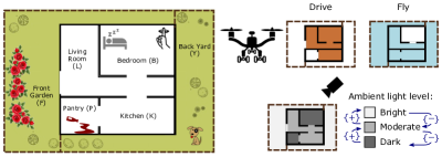
Figure 1: A hybrid drone with a light sensor monitors a home. The robot is capable of driving or flying: the grass outdoors (F and Y) and liquids (P) necessitate that it be airborne; the noise requirement means it may only drive within the bedroom (B). It has a light sensor that distinguishes three levels of ambient brightness. Changes in brightness (increasing ‘$+$’, decreasing ‘$-$’, same ‘$=$’) provide the robot cues about its location.

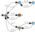
(a) A naïve filter, with one state per region, codifies all valid choices.

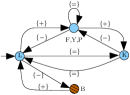
(b) A minimal filter when choosing to fly in the living room (L) and kitchen (K).

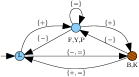
(c) A minimal filter when opting to fly in the living room (L) but not the kitchen (K).

Figure 2: Combinatorial filters that tell the hybrid drone how to locomote. The sequence of symbols  $\{$$+$,$-$,$=$$\}$  is traced on the graph, and the color of the resultant state is the filter’s output (blue for flight, brown for driving mode).

We wish to construct a filter for the drone to determine how to navigate, with the inputs being brightness changes, and the filter’s output providing some valid mode of locomotion. It is easy to give a valid filter by using one state for each location — this naïve filter is depicted in Figure 2(a). In the living room and kitchen, the filter lists two outputs since both modes are applicable there (both locations are covered by the brown and blue choices). Now consider the question of the smallest filter. If we opt to fly in both the living room and kitchen, then the smallest filter is shown in Figure 2(b) with $4$ states. But when choosing to fly in the living room but drive in the kitchen, the minimal filter requires only $3$ states (in Figure 2(c)).

This last filter is also the globally minimal filter. The crux is that states with multiple valid outputs introduce a new degree of freedom which influences the size of the minimal filter. These arise, for instance, whenever there are ‘don’t-care’ options. The flexibility of such states must be retained to truly minimize the number of states.

2 Preliminary Definitions and Problem Description

To begin, we define the filter minimization problem in the most general form, where the input is allowed to be non-deterministic and each state may have multiple outputs. This is captured by the procrustean filter (p-filter) formalism [6].

2.1 P-filters and their minimization

We firstly introduce the notion of p-filter:

Definition 1 (procrustean filter [6]).

A procrustean filter, p-filter or filter for short, is a tuple $(V,V_{0},Y,\tau,C,c)$ with:

• a finite set of states $V$, a non-empty initial set of states $V_{0}\subseteq V$, and a set of possible observations $Y$,

• a transition function $\tau:V\times V\rightarrow 2^{Y}$,

• a set $C$, which we call the output space, and

• an output function $c:V\to 2^{C}\setminus\{\varnothing\}$.

The states, initial states and observations for p-filter $F$ will be denoted $V(F)$, $V_{0}(F)$ and $Y(F)$. Without loss of generality, we will also treat a p-filter as a graph with states as its vertices and transitions as directed edges.

A sequence of observations can be traced on the p-filter:

Definition 2 (reached).

Given any p-filter $F=(V,V_{0},Y,\tau,C,c)$, a sequence of observations $s=y_{1}\dots y_{n}\in Y^{*}$, and states $w_{0},w_{n}\in V$, we say that $w_{n}$ is a state reached by some sequence $s$ from $w_{0}$ in $F$ (or $s$ reaches $w_{n}$ from $w_{0}$), if there exists a sequence of states $w_{0},\dots,w_{n}$ in $F$, such that $\forall i\in\{1,\dots,n\},y_{i}\in\tau(w_{i-1},w_{i})$. We denote the set of all states reached by $s$ from state $w_{0}$ in $F$ as $\mathcal{V}_{w_{0}}(F,s)$. For simplicity, we use $\mathcal{V}(F,s)$, without the subscript, to denote the set of all states reached when starting from any state in $V_{0}$, i.e., $\mathcal{V}(F,s)=\cup_{v_{0}\in V_{0}}\mathcal{V}_{v_{0}}(F,s)$. Note that $\mathcal{V}(F,s)=\varnothing$ holds only when sequence $s$ crashes in $F$ starting from $V_{0}$.

For convenience, we will denote the set of sequences reaching state $v\in V$ from some initial state by $\mathcal{S}^{F}_{v}$.

Definition 3 (extensions, executions and interaction language).

An extension of a state $v$ on a p-filter $F$ is a finite sequence of observations $s$ that does not crash when traced from $v$, i.e., $\mathcal{V}_{v}(F,s)\neq\varnothing$. An extension of any initial state $v_{0}\in V_{0}(F)$ is also called an execution or a string on $F$. The set of all extensions of a state $v$ on $F$ is called the extensions of $v$, written as $\mathcal{L}_{F}(v)$. The extensions of all initial vertices on $F$ is also called the interaction language (or, briefly, just language) of $F$, and is written $\mathcal{L}(F)=\cup_{v_{0}\in V_{0}(F)}\mathcal{L}_{F}(v_{0})$.

Note in particular that the empty string $\epsilon$ belongs to the extensions of any state on the filter, and belongs to the language of the filter as well.

Definition 4 (filter output).

Given any p-filter $F=(V,V_{0},Y,\tau,C,c)$, a string $s$ and an output $o\in C$, we say that $o$ is a filter output with input string $s$, if $o$ is an output from the state reached by $s$, i.e., $o\in\cup_{v\in\mathcal{V}(F,s)}c(v)$. We denote the set of all filter outputs for string $s$ as $\mathcal{C}(F,s)=\cup_{v\in\mathcal{V}(F,s)}c(v)$.

Specifically, for the empty string $\epsilon$, we have $\mathcal{C}(F,\epsilon)=\cup_{v_{0}\in V_{0}(F)}c(v_{0})$.

Definition 5 (output simulating).

Given any p-filter $F$, a p-filter $F^{\prime}$ output simulates $F$ if $\forall s\in\mathcal{L}(F)$, $\mathcal{C}(F^{\prime},s)\neq\varnothing$ and $\mathcal{C}(F^{\prime},s)\subseteq\mathcal{C}(F,s)$.

Plainly in words: for one p-filter to output simulate another, it has to generate some of the outputs of the other, for every string the other admits.

We are interested in practicable p-filters with deterministic behavior:

Definition 6 (deterministic).

A p-filter $F=(V,V_{0},Y,\tau,C,c)$ is deterministic or state-determined, if $|V_{0}|=1$, and for every $v_{1},v_{2},v_{3}\in V$ with $v_{2}\neq v_{3}$, $\tau(v_{1},v_{2})\cap\tau(v_{1},v_{3})=\varnothing$.

Any non-deterministic p-filter $F$ can be state-determinized, denoted $\operatorname{\textsc{Sde}}({F})$, following Algorithm $2$ in [7].

Then the p-filter minimization problem can be formalized as follows:

Problem: P-filter Minimization (pfm) Input: A deterministic p-filter $F$. Output: A deterministic p-filter $F^{\dagger}$ with fewest states, such that $F^{\dagger}$ output simulates $F$.

‘pf’ denotes that the input is a p-filter, and ‘m’ denotes that we are interested in finding a deterministic minimal filter as a solution.

2.2 Complexity of p-filter minimization problems

Definition 7 (state single-outputting and multi-outputting).

A p-filter $F=(V,V_{0},Y,\tau,C,c)$ is state single-outputting or single-outputting for short, if $c$ only maps to singletons, i.e., $|c(v)|=1,\forall v\in V(F)$. Otherwise, we say that $F$ is multi-outputting.

Depending on whether the state in the input p-filter (pf) is single-outputting (so) or multi-outputting (mo), we further categorize the problem pfm into the following problems: so-fm and mo-fm.

Lemma 8.

The filter minimization problem fm of [5] is so-fm, and so-fm is NP-Complete (Theorem $2$ in [5]).

Theorem 9.

mo-fm is NP-Complete.

Proof.

Firstly, so-fm is a special case of mo-fm problems. These mo-fm problems are at least as hard as so-fm. Hence, mo-fm are in NP-hard. On the other hand, a solution for mo-fm can be verified in polynomial time. (Change the equality check on line 7 of Algorithm 1 in [5] to a subset check.) Therefore, mo-fm is NP-Complete. ∎

Next, we examine related prior work on so-fm closely as a means to develop new insights for our algorithms, first for so-fm (Section 4), and then mo-fm (Section 5).

3 Related work: Prior filter minimization ideas (so-fm)

Several elements come together in this section and Figure 3 attempts to show the inter-relationships graphically. The original question of minimizing state in filtering is first alluded to by LaValle [4] as an open problem, who suggested that it is ‘similar to Nerode equivalence classes’. The problem of filter reduction, i.e., so-fm in our terms, was formalized and shown to differ in complexity class from the automata problem in [5]. That paper also proposed a heuristic algorithm, which served as a starting point for subsequent work. The heuristic algorithm uses conflict graphs to designate which vertices cannot be merged (are conflicting). It starts with a conflict relation where two vertices are in conflict when they have different outputs, then iteratively refines the conflict relation. Refinement has two steps: ($i$) introducing edges: two vertices are determined to be conflicting or not via a graph coloring subroutine, and edges are added between conflicting vertices; ($ii$) propagating conflicts upstream: filter states are marked as conflicted when they transition to conflicted states under the same observation. An example input filter, shown in Figure 4(a), is reduced by following this procedure, which is depicted step-by-step in Figures 4(b)–4(e).

A conjecture in [5] was that this algorithm is guaranteed to find a minimal filter if the graph coloring subroutine gives a minimal coloring. (Put another way: the inexactness in arriving at a minimal filter can be traced to the graph coloring giving a suboptimal result.) But this conjecture was later proved to be false by Saberifar et al. [8]. They show an instance where there exist multiple distinct optimal solutions to the graph coloring subproblem, only a strict subset of which lead to the minimal filter. One might naturally ask, and indeed they do ask, the question of whether some optimal coloring is sufficient to arrive at the optimal filter. Following along these lines (see §7.3 in [8]), one might sharpen the original conjecture of [5] to give the following statement:

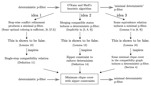
Figure 3: Three distinct insights led to the development of a new algorithm (described in Section 4) for so-fm. This roadmap shows the provenance of those insights in terms of previous ideas in so-fm, which we examine carefully.

Idea 1.

In the step-wise conflict refinement procedure of O’Kane and Shell’s heuristic algorithm [5], some optimal coloring is sufficient to guarantee a minimal filter for so-fm.

Lemma 10.

Idea 1 is false.

Proof.

This is simply shown with a counterexample. Consider the problem of minimizing the input filter shown in Figure 4(a), the heuristic algorithm will first initialize the colors of the vertices with their output. Next, it identifies the vertices that disagree on the outputs of extensions with length $1$ as shown in Figure 4(b), and then refines the colors of the vertices as shown in Figure 4(c) following a minimal graph coloring solution on the conflict graph. Then it further identifies the conflicts on extensions with length $2$, via the conflict graph shown in Figure 4(d), and the vertex colors are further refined as shown in Figure 4(e). Now, no further conflicts can be found. A filter, with $6$ states, is then obtained by merging the states with the same color. However, there exists a minimal filter, with $5$ states, shown in Figure 4(f), that can be found by choosing coloring solution for the conflict graph shown in Figure 4(b). That coloring is suboptimal. ∎

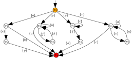
(a) Example input p-filter.

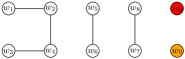
(b) Graphs of initial conflicts for all vertices with the same output.

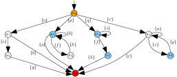
(c) The first refinement of the filter following an optimal coloring of the conflict graphs.

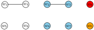
(d) Reduced conflict graphs.

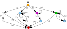
(e) Second refinement of filter following an optimal coloring of the conflict graphs.

(f) The coloring that gives the minimal filter.

Figure 4: An example run of the heuristic minimization algorithm in [5] (a)–(e). This particular input also shows that optimal step-wise conflict refinement may fail to yield a minimal filter (Lemma 10).

This appears to indicate a sort of local optimum arising via sub-problems associated with incremental (or stepwise) reduction. Since optimal colorings for individual steps are seen to be insufficient to guarantee a minimal filter, to find a minimal filter, we would have to enumerate all colorings (suboptimal or otherwise) at each iteration. That is, however, essentially a brute force algorithm. A more informed approach is to compute implications of conflicts more globally, in a way that doesn’t depend on earlier merger decisions. In our algorithm, rather than tracking vertices which are in conflict, we introduce a new notion of compatibility between vertices that may be merged. This notion differs from the one recursively defined in [9], as our compatibility relation is computed in one fell swoop, before making any decisions to reduce the filter:

Definition 11 (compatibility).

Let $F$ be a deterministic p-filter. We say a pair of vertices $v,w\in V(F)$ are compatible, denoted $v\sim_{c}w$, if they agree on the outputs of all their extensions, i.e., $\forall s\in\mathcal{L}_{F}(v)\cap\mathcal{L}_{F}(w),\forall v^{\prime}\in\mathcal{V}_{v}(F,s),\forall w^{\prime}\in\mathcal{V}_{w}(F,s),c(v^{\prime})=c(w^{\prime})$. A mutually compatible set consists of vertices where all pairs are compatible.

Via this notion of compatibility, we get an undirected compatibility graph:

Definition 12 (compatibility graph).

Given a deterministic filter $F$, its compatibility graph $\mathcal{K}(F)$ is an unlabeled undirected graph constructed by creating a vertex associated with each state in $F$, and building an edge between the pair of vertices associated with two compatible states.

This compatibility graph can be constructed in polynomial time. As every filter state and associated compatibility graph state are one-to-one, to simplify notation we’ll use the same symbol for both and context to resolve any ambiguity.

The second idea relates to the type of the output one obtains after merging states that are compatible or not in conflict. Importantly, the filter minimization problem so-fm requires one to give a minimal filter which is deterministic.

Idea 2.

By merging the states that are compatible, the heuristic algorithm always produces a deterministic p-filter.

The definition of the reduction problems within [5, 8, 9] are specified so as to require that the output obtained be deterministic. But this postcondition is never shown or formally established. In fact, it does not always hold.

Lemma 13.

Idea 2 is false.

Proof.

We show that the existing algorithm may produce a non-deterministic filter, which does not output simulate the input filter, and is thus not a valid solution. Consider the filter shown in Figure 5(a) as an input. The vertices with the same color are compatible with each other, with the following exception for $w_{5}$, $w_{6}$ and $w_{7}$. Vertex $w_{5}$ is compatible with $w_{6}$, vertex $w_{6}$ is compatible with $w_{7}$, but $w_{5}$ is not compatible with $w_{7}$. The minimal filter found by the existing algorithm is shown in Figure 5(b). The string $aac$ suffices to shows the non-determinism, reaching both orange and cyan vertices. It fails to output simulate the input because cyan should never be produced. ∎

If determinism can’t be taken for granted, we might constrain the output to ensure the result will be a deterministic filter. To do this, we introduce a zipper constraint when merging compatible states:

Definition 14 (zipper constraint).

In the compatibility graph $G=\mathcal{K}(F)$ of filter $F$, if there exists a set of mutually compatible states $U=\{u_{1},u_{2},\dots,u_{n}\}$, then they can only be selected to be merged if they always transition to a set of states that are also selected to be merged. For any sets of mutually compatible states $U,W\subseteq V(G)$ and some observation $y$, we create a zipper constraint expressed as a pair $(U,W)_{y}$ if $W=\left\{w\in V(G)\mid y\in\tau(u,w)\text{ for some }u\in U\right\}$. We denote the set of all zipper constraints on compatibility graph $G=\mathcal{K}(F)$ by $\mathscr{Z}(F)$.

The zipper constraints for the input filter shown in Figure 5(a) consist of $(\{w_{1},w_{2}\},\{w_{5},w_{6}\})_{a}$ and $(\{w_{3},w_{4}\},\{w_{6},w_{7}\})_{b}$. Constraint $(\{w_{1},w_{2}\},\{w_{5},w_{6}\})_{a}$ is interpreted as: if $w_{1}$ and $w_{2}$ are selected for merger, then $w_{5}$ and $w_{6}$ (reached under $a$) should also be merged. We call it a zipper constraint owing to the resemblance to a zipper fastener: merger of two earlier states, merges (i.e., pulls together) later states. In the worst case, the number of zipper constraints can be exponential in the size of the input filter.

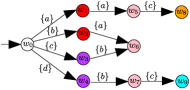
(a) An input filter.

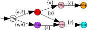
(b) The non-deterministic minimal filter found by the existing algorithm.

Figure 5: A counterexample showing how compatible merges may introduce non-determinism (Lemma 13). The input filter also illustrates a violation of the presumption that an equivalence relation can yield a minimum filter (Lemma 16).

A third idea is used by O’Kane and Shell’s heuristic algorithm and is also stated, rather more explicitly, by Saberifar et al. (see Lemma 5 in [8] and Lemma $5$ in [9]). It indicates that we can obtain a minimal filter via merging operations on the compatible states, which yields a special class of filter minimization problems. For this class, recent work has expoited integer linear programming techniques to compute exact and feasible solutions efficiently [10].

Idea 3.

Some equivalence relation induces a minimal filter in so-fm.

Before examining this, we rigorously define the notion of an induced relation:

Definition 15 (induced relation).

Given a filter $F$ and another filter $F^{\prime}$, if $F^{\prime}$ output simulates $F$, then $F^{\prime}$ induces a relation $R\subseteq V(F)\times V(F)$, where $(v,w)\in R$ if and only if there exists a vertex $v^{\prime}\in V(F^{\prime})$ such that $\mathcal{S}^{F}_{v}\cap\mathcal{S}^{F^{\prime}}_{v^{\prime}}\neq\varnothing$ and $\mathcal{S}^{F}_{w}\cap\mathcal{S}^{F^{\prime}}_{v^{\prime}}\neq\varnothing$. We also say that $v$ and $w$ corresponds to state $v^{\prime}$.

Lemma 16.

Idea 3 is false.

Proof.

It is enough to scrutinize the previous counterexample closely. The minimization problem so-fm for the input filter shown in Figure 5(a), is shown in Figure 6(a). It is obtained by ($i$) splitting vertex $w_{6}$ into an upper part reached by $a$ and a lower part reached by $b$, ($ii$) merging the upper part of $w_{6}$ with $w_{5}$, the lower part of $w_{6}$ with $w_{7}$, and other vertices with those of the same color. This does not induce an equivalence relation, since $w_{6}$ corresponds to two different vertices in the minimal filter. ∎

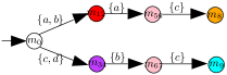
(a) A minimal filter for Figure 5(a).

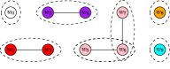
(b) Cliques from the minimal filter.

Figure 6: A minimal filter for Figure 5(a) and its induced cliques.

In light of this, for some filter minimization problems, there may be no quotient operation that produces a minimal filter and an exact algorithm for minimizing filters requires that we look beyond equivalence relations.

Some strings that reach a single state in an input filter may reach multiple states in a minimal p-filter (e.g., $ba$ and $cb$ on Figure 5(a) and 6(a)). On the other hand, strings that reach different states in the input p-filter may reach the same state in the minimal filter (e.g., $a$ and $b$ on those same filters). We say that a state from the input filter corresponds to a state in the minimal filter if there exists some string reaching both of them and, hence, this correspondence is many-to-many. An important observation is this: for each state $s$ in some hypothetical minimal filter, suppose we collect all those states in the input filter that correspond with $s$. When we examine the associated states in the compatibility graph for that collection, they must all form a clique. Were it not so, the minimal filter could have more than one output associated for some strings owing to non-determinism. But this causes it to fail to output simulate the input p-filter.

After firming up and developing these intuitions, the next section introduces the concept of a clique cover which enables representation of a search space that includes relations more general than equivalence relations. Based on this new representation, we propose a graph problem use of zipper constraints, and prove it to be equivalent to filter minimization.

4 A new graph problem that is equivalent to so-fm

By building the correspondence between the input p-filter in Figure 5(a) and the minimal result in Figure 6(a), one obtains the set of cliques in the compatibility graph shown visually in Figure 6(b). Like previous approaches that make state merges by analyzing the compatibility graph, we interpret each clique as a set of states to be merged into one state in the minimal filter. The clique containing $w_{3}$ and $w_{4}$ in Figure 6(b) gives rise to $m_{34}$ in the minimal filter in Figure 6(a) (and $w_{1}$ and $w_{2}$ yields $m_{12}$, and so on). However, states may further be shared across multiple cliques. We observe that $w_{6}$ was merged with $w_{5}$ in the minimal filter to give $m_{56}$, and $w_{6}$ also merged with $w_{7}$ to give $m_{67}$. The former has an incoming edge labeled with an $a$, while the latter has an incoming edge labeled $b$. The vertex $w_{6}$, being shared by multiple cliques, is split into different copies and each copy merged separately.

Generalizing this observation, we turn to searching for the smallest set of cliques that cover all vertices in the compatibility graph. Further, to guarantee that the set of cliques induces a deterministic filter, we must ensure they respect the zipper constraints. It will turn out that a solution of this new constrained minimum clique cover problem always induces a minimal filter for so-fm, and a minimal filter for so-fm always induces a solution for this new problem. The final step is to reduce any mcczc problem to a SAT instance, and leverage SAT solvers to find a minimal filter for so-fm.

4.1 A new minimum clique cover problem

To begin, we extend the preceding argument from the compatibility clique associated to single state $s$, over to all the states in the minimal filter. This leads one to observe that the collection of all cliques for each state in the minimal p-filter forms a clique cover:

Definition 17 (induced clique cover).

Given a p-filter $F$ and another p-filter $F^{\prime}$, we say that a vertex $v$ in $F$ corresponds to a vertex $v^{\prime}_{i}$ in $F^{\prime}$ if $\mathcal{S}^{F}_{v}\cap\mathcal{S}^{F^{\prime}}_{v^{\prime}_{i}}\neq\varnothing$. Then, denoting the subset of vertices of $F$ corresponding to $v^{\prime}_{i}$ in $F^{\prime}$ with $K_{v^{\prime}_{i}}=\{v\in V(F)\,|\,v\text{ corresponds to }v^{\prime}_{i}\}$, we form the collection of all such sets, $\mathbf{Q}(F,F^{\prime})=\{K_{v^{\prime}_{1}},K_{v^{\prime}_{2}},\dots,K_{v^{\prime}_{n}}\}$, for $i\in\{1,\dots,n\}$ where $n=|V(F^{\prime})|$. When $F^{\prime}$ output simulates $F$, then the $K_{v^{\prime}_{i}}$ form cliques in the compatibility graph $\mathcal{K}(F)$. Further, when this collection of sets $\mathbf{Q}(F,F^{\prime})$ covers all vertices in $F$, i.e., $\cup_{K_{i}\in\mathbf{Q}(F,F^{\prime})}=V(F)$, we say that $\mathbf{Q}(F,F^{\prime})$ is an induced clique cover.

It is worth repeating: the size of filter $F^{\prime}$ (in terms of number of vertices) and the size of the induced clique cover (number of sets) are equal.

Without loss of generality, here and henceforth we only consider the p-filter with all vertices reachable from the initial state, since the ones that can never be reached will be deleted during filter minimization anyway.

Each clique of the clique cover represents the states that can be potentially merged. But the zipper constraint, to enforce determinism, requires that the set of vertices to be merged should always transition under the same observation to the ones that can also be merged. Hence, the zipper constraints (of Definition 14) can be evaluated across whole covers:

Definition 18.

A clique cover $\mathbf{K}=\{K_{0},K_{1},\dots,K_{m}\}$ satisfies the set of zipper constraints $\textsc{Zip}=\{(U_{1},W_{1})_{y_{1}},(U_{2},W_{2})_{y_{2}},\dots\}$, when for every zipper constraint $(U_{i},W_{i})_{y_{i}}$, if there exist a clique $K_{s}\in\mathbf{K}$, such that $U_{i}\subseteq K_{s}$, then there exists another clique $K_{t}\in\mathbf{K}$ such that $W_{i}\subseteq K_{t}$.

Now, we have our new graph problem, mcczc.

Problem: Minimum clique cover with zipper constraints (mcczc) Input: A compatibility graph $G$, a set of zipper constraints Zip. Output: A minimal cardinality clique cover of $G$ satisfying Zip.

4.2 From minimal clique covers to filters

Given a minimal cover that solves mcczc, we construct a filter by merging the states in the same clique and choosing edges between these cliques appropriately:

Definition 19 (induced filter).

Given a clique cover $\mathbf{K}$ on the compatibility graph of deterministic p-filter $F$, if $\mathbf{K}$ satisfies all the zipper constraints in $\mathscr{Z}(F)$, then it induces a filter $F^{\prime}=M(F,\mathbf{K})$ by treating cliques as vertices:

1. Create a new filter $F^{\prime}=(V^{\prime},V^{\prime}_{0},Y,\tau^{\prime},C,c^{\prime})$ with $|\mathbf{K}|$ vertices, where each vertex $v^{\prime}$ is associated with a clique $K_{v^{\prime}}$ in $\mathbf{K}$;

2. Add each vertex $v^{\prime}$ in $F^{\prime}$ to $V^{\prime}_{0}$ iff the associated clique contains an initial state in $F$;

3. The output of every $v^{\prime}$ in $F^{\prime}$, with associated clique $K_{v^{\prime}}$, is the set of common outputs for all states in $K_{v^{\prime}}$, i.e., $c^{\prime}(v^{\prime})=\cap_{v\in K_{v^{\prime}}}c(v)$.

4. For any pair of $v^{\prime}$ and $w^{\prime}$ in $F^{\prime}$, inherit all transitions between states in the cliques of $v^{\prime}$ and $w^{\prime}$, i.e., $\tau(v^{\prime},w^{\prime})=\cup_{v\in K_{v^{\prime}},w\in K_{w^{\prime}}}\tau(v,w)$.

5. For each vertex $v^{\prime}$ in $F^{\prime}$ with multiple outgoing edges labeled $y$, keep only the single edge to the vertex $w^{\prime}$, such that all vertices $K_{v^{\prime}}$ transition to under $y$ are included in $K_{w^{\prime}}$. This edge must exist since $\mathbf{K}$ satisfies all $\mathscr{Z}(F)$.

The size of the cover (in terms of number of sets) and size of the induced filter (number of vertices) are equal.

Notice that the earlier intuition is mirrored by this formal construction: states belonging to the same clique are merged when constructing the induced filter; states in multiple cliques are split when we make the edge choice in step 5. Next, we establish that the induced filter indeed supplies the goods:

lemmadeterministicouputsimulating Given any clique cover $\mathbf{K}$ on the compatibility graph $\mathcal{K}(F)$ of a deterministic p-filter $F$, if $\mathbf{K}$ satisfies the zipper constraints $\mathscr{Z}(F)$ and covers all vertices of $\mathcal{K}(F)$, then the induced filter $F^{\prime}=M(F,\mathbf{K})$ is deterministic and output simulates $F$.

Proof.

For any string $s\in\mathcal{L}(F)$, let the vertex reached by string $s$ in $F$ be $v$. Then $v$ must belong at least one clique in $\mathbf{K}$, where all vertices in this clique can be viewed as merged into a new vertex in $F^{\prime}$. Hence, $s$ should reach at least one vertex in $F^{\prime}$ and this vertex yield the same output $\mathcal{C}(F,s)$. Since $\mathbf{K}$ satisfies the zipper constraints $\mathscr{Z}(F)$, the induced filter $F^{\prime}$ must be deterministic since there is no vertex that has any non-deterministic outgoing edges bearing the same label. Because $F^{\prime}$ is deterministic, $\forall s\in\mathcal{L}(F)$, $s$ reaches a single vertex in $F^{\prime}$. In addition, this vertex in $F^{\prime}$ shares the same output $\mathcal{C}(F,s)$. Therefore, $F^{\prime}$ also output simulates $F$. ∎

A surprising aspect of the preceding is how the zipper constraints  —which are imposed to ensure that a deterministic filter is produced— enforce output-simulating behavior, albeit indirectly, too. One might have expected that this separate property would demand a second type of constraint, but this is not so.

On the other hand, needing to satisfy the zipper constraints of the input filter does not entail the imposition of any gratuitous requirements:

lemmacliqueaux Given any deterministic p-filters $F$ and $F^{\prime}$, if $F^{\prime}$ output simulates $F$, then the induced clique cover $\mathbf{Q}(F,F^{\prime})$ on the compatibility graph of $F$ satisfies all zipper constraints in $\mathscr{Z}(F)$.

Proof.

Suppose that $\mathbf{Q}(F,F^{\prime})$ does not satisfy all zipper constraints in $\mathscr{Z}(F)$. Specifically, let $(U,V)_{y}\in\mathscr{Z}(F)$ be the zipper constraint that is violated, where each vertex in $V$ transitions from some vertex in $U$ under observation $y$. Then there exists a clique $K_{s}\in\mathbf{Q}(F,F^{\prime})$, such that $U\subseteq K_{s}$, but there is no clique $K_{j}\in\mathbf{Q}(F,F^{\prime})$ that $V\subseteq K_{j}$. According to the construction of the induced cover, there exists a vertex $v^{\prime}_{s}\in F^{\prime}$, such that $K_{s}$ corresponds to $v^{\prime}_{s}$. For any vertex $u_{1}\in K_{s}$, let $s_{1}\in\mathcal{S}^{F}_{u_{1}}\cap\mathcal{S}^{F^{\prime}}_{v^{\prime}_{s}}$. Then $s_{1}y$ is also a string in both $F$ and $F^{\prime}$ since $u_{1}$ transitions to some vertex $v_{1}$ in $V$ under observation $y$ in $F$ and $F^{\prime}$ is output simulating $F^{\prime}$. Let $\mathcal{V}(F^{\prime},s_{1}y)=\{v^{\prime}_{t}\}$. (It is a singleton set as $F^{\prime}$ is deterministic.) Hence $v_{1}$ corresponds to $v^{\prime}_{t}$ on common string $s_{1}y$. Similarly, each vertex $v\in V$ corresponds to $v^{\prime}_{t}$ on some string ending with $y$. Let the clique corresponding to $v^{\prime}_{t}$ be $K_{t}$, and we have $K_{t}\supseteq V$. But that is a contradiction. ∎

4.3 Correspondence of mcczc and so-fm solutions

To establish the equivalence between mcczc and so-fm, we will show that the induced filter from the solution of mcczc is a minimal filter for so-fm, and the induced clique cover from a minimal filter is a solution for mcczc.

Lemma 20.

Minimal clique covers for mcczc induce minimal filters for so-fm.

Proof.

Given any minimal clique cover $\mathbf{K}=\{K_{1},K_{2},\dots,K_{m}\}$ as a solution for problem mcczc with input p-filter $F$, construct p-filter $F^{\prime}=M(F,\mathbf{K})$. Since $\mathbf{K}$ satisfies the zipper constraints $\mathscr{Z}(F)$, $F^{\prime}$ is deterministic and output simulates $F$ according to Lemma 19. To show that $F^{\prime}$ is a minimal deterministic filter for so-fm, suppose the contrary. Then there exists a minimal deterministic filter $F^{\star}$ with fewer states, i.e., $|V(F^{\star})|<|V(F^{\prime})|$. Hence, $F^{\star}$ induces a clique cover $\mathbf{K^{\star}}$ with fewer cliques than $\mathbf{K}$. Since $F^{\star}$ is deterministic, $\mathbf{K^{\star}}$ satisfies all $\mathscr{Z}(F)$ via Lemma 19. But then $\mathbf{K^{\star}}$ satisfies all the requirements to be a solution for mcczc, and has fewer cliques than $\mathbf{K}$, contradicting the assumption. ∎

Lemma 21.

A minimal filter for so-fm with input $F$ induces a clique cover that solves mcczc with compatibility graph and zipper constraints of $F$.

Proof.

Given minimal filter $F^{\star}$ as a solution for so-fm with input filter $F$, we can construct a clique cover $\mathbf{K}=\mathbf{Q}(F,F^{\star})$ from the minimal filter. For this cover to be a solution for mcczc with compatibility graph $G=\mathcal{K}(F)$ and zipper constraints $\mathscr{Z}(F)$, first, it must satisfy all constraints in $\mathscr{Z}(F)$. Lemma 19 affirms this fact. Second, we must show it to be minimal among all the covers satisfying those constraints. Supposing $\mathbf{K}$ is not a minimal, there must exist a clique cover $\mathbf{K^{\prime}}$ with $|\mathbf{K^{\prime}}|<|\mathbf{K}|$ satisfying $\mathscr{Z}(F)$. Then, consider the induced filter $F^{\prime}=M(F,\mathbf{K^{\prime}})$. Since $\mathbf{K^{\prime}}$ satisfies all the zipper constraints $\mathscr{Z}(F)$, $F^{\prime}$ is deterministic and will output simulate $F$ (Lemma 19). But $|V(F^{\prime})|=|\mathbf{K^{\prime}}|<|\mathbf{K}|=|V(F^{\star})|$, contravening the fact that $F^{\star}$ is a minimal filter. Hence $\mathbf{K}$ is minimal. ∎

Together, they establish the theorem.

Theorem 22.

The solution for mcczc with compatibility graph and zipper constraints of a filter $F$ induces a solution for so-fm with input filter $F$, and vice versa.

Proof.

Lemma 20 and Lemma 21 comprise the complete result. ∎

Having established this correspondence, any so-fm can be solved by tackling its associated mcczc problem, the latter problem being cast as a SAT instance and solved via a solver (see Section 6 for further details).

5 Generalizing to mo-fm

Finally, we generalize the previous algorithm to multi-outputting filters. In mo-fm problems, the input p-filter is deterministic but states in the p-filter may have multiple outputs. One straightforward if unsophisticated approach is to enumerate all filters under different output choices for the states with multiple outputs, and then solve every one the resulting deterministic single-outputting filters as instances of so-fm. The filter with the fewest states among all the minimizers could then be treated as a minimal one for the mo-fm problem.

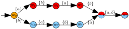
(a) An input filter with multi-outputting states. The colors in each vertex represents its output.

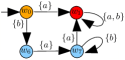
(b) A minimal filter when choosing to output the same color for $w_{4}$ and $w_{5}$.

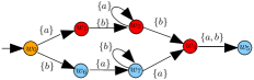
(c) A minimal filter when choosing to output different colors for $w_{4}$ and $w_{5}$.

(d) A minimal filter for the input filter.

Figure 7: A multi-outputting filter minimization problem.

Unfortunately, this is too simplistic. Prematurely committing to an output choice is detrimental. Consider the input filter shown in Figure 7(a), it has two multi-outputting states ($w_{4}$ and $w_{5}$). If we choose to have both $w_{4}$ and $w_{5}$ give the same output, the so-fm minimal filter, shown in Figure 7(b), has $4$ states. If we choose distinct outputs for $w_{4}$ and $w_{5}$, the so-fm minimal filter, shown in Figure 7(c), now has $7$ states. But neither is the minimal mo-fm filter. The true minimizer appears in Figure 7(d), with only $3$ states. It is obtained by splitting both $w_{4}$ and $w_{5}$ into two copies, each copy giving a different output.

The idea underlying a correct approach is that output choices should be made together with the splitting and merging operations during filter minimization. Multi-outputting vertices may introduce additional split operations, but these split operations can still be treated via clique covers on the compatibility graph. This requires that we define a new compatibility relationship—it is only slightly more general than Definition 11:

Definition 23 (group compatibility).

Let $F$ be a deterministic p-filter. We say that the set of states $U=\{u_{1},u_{2},\dots,u_{n}\}$ are group compatible, if there is a common output on all their extensions, i.e.,

$$\forall s\in\bigcup\limits_{u\in U}\mathcal{L}_{F}(u),\bigcap\limits_{w^{\prime}\in W^{\prime}}\!c(w^{\prime})\neq\varnothing,\text{ where }W^{\prime}=\mathcal{V}_{u_{1}}(F,s)\cup\mathcal{V}_{u_{2}}(F,s)\cup\cdots\mathcal{V}_{u_{n}}(F,s).$$

(The preceding exploits the subtle fact, in Definition 3, that $\mathcal{V}_{v}(F,s)=\varnothing$ when tracing $s$ from $v$ crashes in $F$.) With this definition, the compatibility graph must be generalized suitably:

Definition 24 (compatibility simplicial complex).

Given a deterministic multi-output filter $F$, its compatibility simplicial complex is a collection of simplices, where each simplex is a set of group compatible vertices in $F$.

The zipper constraints are generalized too, replacing mutual compatibility with group compatible states:

Definition 25 (generalized zipper constraint).

In the compatibility simplicial complex of filter $F$, if there exists a set of group compatible states $U=\{u_{1},u_{2},\dots,u_{n}\}$, then they can only be selected to be merged if they always transition to a set of states that are also selected to be merged. For any sets of group compatible states $U,W\subseteq V(G)$ and some observation $y$, we create a generalized zipper constraint expressed as a pair $(U,W)_{y}$ if $W=\{w\in V(G)\mid y\in\tau(u,w)$ for some $u\in U\}$.

The information formerly encoded in cliques of edges is now within simplicies; the minimum clique cover on the compatibility graph, thus, becomes a minimum simplex cover on the compatibility simplicial complex. Hence, the mcczc problem is generalized as follows:

Problem: Generalized Minimum Cover with zipper constraints (gmczc) Input: A compatibility simplicial complex $M$, a set of generalized zipper constraints Zip. Output: A minimal cardinality simplex cover of $M$ satisfying Zip.

6 Reduction from mcczc and gmczc to SAT

Prior algorithms for filter minimization used multiple stages to find a set of vertices to merge, solving a graph coloring problem repeatedly as more constraints are identified. In contrast, an interesting aspect of mcczc and its generalized version is that it tackles filter minimization as a constrained optimization problem with all constraints established upfront. Thus the clique (simplex) perspective gives an optimization problem which is tangible and easy to visualize. Still, being a new invention, there are no solvers readily available for direct use. But reducing mcczc (gmczc) to Boolean satisfaction (SAT) enables the use of state-of-the-art solvers to find minimum cliques (simplices).

Since the edges that make up the cliques can be encoded via 1-simplices, in what follows we give the treatment of gmczc.

Next, we follow the standard practice for treating optimization problems via a decision problem oracle, viz. define a $k$-gmczc problem, asking for the existence of a cover with size $k$ satisfying the zipper constraints; one then decreases $k$ to find the minimum cover. Each $k$-gmczc problem can be written as a logic formula in conjunctive normal form (CNF), polynomial in the size of the $k$-gmczc instance, and solved.

Firstly, the $k$-gmczc problem is formalized as follows:

Problem: Minimum simplex cover with zipper constraints ($k$-gmczc) Input: A compatibility simplicial complex $M$, a set of zipper constraints Zip, maximum number of simplices $k$ Output: A simplex cover with no more than $k$ simplices on $M$ that satisfies all zipper constraints in Zip

Then, we represent the simplex cover as choices to assign each vertex $v$ in the compatibility simplicial complex to a simplex $i$, with $1\leq i\leq k$. To represent these choices, we create a boolean variable $R_{v}^{i}$ to represent the fact that $v$ is assigned to simplex $i$, and its negation $\overline{R_{v}^{i}}$ to represent its inverse. The simplex cover is captured by $k\times|V(M)|$ such variables.

A simplex cover for problem $k$-gmczc should guarantee that each vertex in $M$ is assigned to at least one clique, i.e.,

$$\prod_{v\in V(M)}\sum_{1\leq i\leq k}R_{v}^{i}.$$ (1)

For simplicity, we will use “$+$” and “$\sum$” for logic or, “$\cdot$” and “$\prod$” for logic and, “$=$” for logic equivalence.

We denote each simplex in the compatibility simplicial complex as a set. Let the set of simplicies for compatibility simplicial complex $M$ be $E(M)$, which is a collection of sets. For any set $\{v_{1},v_{2},\dots,v_{n}\}$ that does not form a simplex in $M$, i.e., $\bar{S}=2^{V(M)}\setminus(E(M)\cup\{\varnothing\})$, they should never be assigned to the same simplex:

$$\prod_{\{v_{1},v_{2},\dots,v_{n}\}\in\bar{S}}\prod_{1\leq i\leq k}(\overline{R_{v_{1}}^{i}}+\overline{R_{v_{2}}^{i}}+\dots+\overline{R_{v_{n}}^{i}}).$$ (2)

To satisfy each zipper constraint $(U,W)_{y}\in\textsc{Zip}$ (with $|U|=m$ and $|W|=n$), if $U$ is assigned to a simplex $i$ ($1\leq i\leq k$), then there must exist another simplex $j$ ($1\leq j\leq k$), such that all vertices in $W$ are assigned to simplex $j$, i.e.,

$$\sum_{1\leq i\leq k}\prod_{u\in U}R_{u}^{i}\implies\sum_{1\leq j\leq k}\prod_{w\in W}R_{w}^{j}$$

$$= \prod_{1\leq i\leq k}\sum_{u\in U}\overline{R_{u}^{i}}+\sum_{1\leq j\leq k}\prod_{w\in W}R_{w}^{j}.$$

Let $X_{i}=\sum_{u\in U}\overline{R_{u}^{i}}$ and $Y=\sum_{1\leq j\leq k}\prod_{w\in W}R_{w}^{j}$, then

$$\prod_{1\leq i\leq k}\sum_{u\in U}\overline{R_{u}^{i}}+\sum_{1\leq j\leq k}\prod_{w\in W}R_{w}^{j}= X_{1}\cdot X_{2}\cdot\,\cdots\,\cdot X_{k}+Y$$

$$= (X_{1}+Y)\cdot(X_{2}+Y)\cdot\,\cdots\,\cdot(X_{k}+Y)$$

$$= \prod_{1\leq i\leq k}(X_{i}+Y).$$

For each $X_{i}+Y$, we have

$$Y+X_{i} =\sum_{1\leq j\leq k}\prod_{w\in W}R_{w}^{j}+\sum_{u\in U}\overline{R_{u}^{i}}$$

$$=\underbrace{R_{w_{1}}^{1}\cdot R_{w_{2}}^{1}\cdot\,\cdots\,\cdot R_{w_{n}}^{1}}_{z^{i}_{1}}+\underbrace{R_{w_{1}}^{2}\cdot R_{w_{2}}^{2}\cdot\,\cdots\,\cdot R_{w_{n}}^{2}}_{z^{i}_{2}}+$$

$$\dots+\underbrace{R_{w_{1}}^{k}\cdot R_{w_{2}}^{k}\cdots R_{w_{n}}^{k}}_{z^{i}_{k}}+\underbrace{\overline{R_{u_{1}}^{i}}\cdot\text{True}}_{z^{i}_{k+1}}+\underbrace{\overline{R_{u_{2}}^{i}}\cdot\text{True}}_{z^{i}_{k+2}}+\dots+\underbrace{\overline{R_{u_{m}}^{i}}\cdot\text{True}}_{z^{i}_{k+m}}$$

$$=(\sum_{1\leq\ell\leq k+m}z^{i}_{\ell})\cdot(\prod_{1\leq j\leq k}\prod_{1\leq p\leq n}(\overline{z^{i}_{j}}+R_{w_{p}}^{j}))\cdot(\prod_{1\leq q\leq m}(\overline{z^{i}_{k+q}}+\overline{R_{u_{q}}^{i}})).$$

Therefore,

$$\prod_{1\leq i\leq k}\sum_{u\in U}\overline{R_{u}^{i}}+\sum_{1\leq j\leq k}\prod_{w\in W}R_{w}^{j}$$ (3)

$$= \prod_{1\leq i\leq k}(X_{i}+Y)$$

$$= \prod_{1\leq i\leq k}\Big{[}(\sum_{1\leq\ell\leq k+m}z^{i}_{\ell})\cdot(\prod_{1\leq j\leq k}\prod_{1\leq p\leq n}(\overline{z^{i}_{j}}+R_{w_{p}}^{j}))\cdot(\prod_{1\leq q\leq m}(\overline{z^{i}_{k+q}}+\overline{R_{u_{q}}^{i}}))\Big{]}.$$

To solve $k$-gmczc, we need to leverage off-the-shelf SAT solvers to find an assignment of the variables such that formulas in (1), (2) and (3) are satisfied. For any vertex in the compatibility graph, we create $k$ variables. For each zipper constraint, we need to create $k(k+m)$ variables. Suppose that there are $t$ vertices in the input filter $F$ and $x$ zipper constraints. Then, we need $tk+xk(k+m)$ variables. Similarly, (1) gives us $1$ clause for each vertex, (2) gives us at most $k\times 2^{t}$ clauses in total, (3) gives $k(k+m+nk+m)$ for each zipper constraint. Hence, the number of clauses to solve a $k$-gmczc is $t+k\times 2^{t}+xk((n+1)k+2m)$.

To find the minimum solution for gmczc, we will solve $k$-gmczc with $k$ equals the number of states in the input filter, and the decrease $k$ until we cannot find a solution for $k$-gmczc (i.e., the SAT solver times out).

7 Experimental results

The method described was implemented by leveraging a Python implementation of 2018 SAT Competition winner, MapleLCMDistChronoBT [12, 13]. Their solver will return a solution if it solves the $k$-mcczc problem before timing out. If it finds a satisfying assignment, we decrease $k$, and try again. Once no satisfying assignment can be found, we construct a minimal filter from the solution with minimum $k$.

First, as a sanity check, we examined the minimization problems for the inputs shown in Figure 2(a), Figure 5(a) and Figure 7(a). Our implementation takes $0.05\text{\,}\mathrm{s}$, $0.06\text{\,}\mathrm{s}$ and $0.26\text{\,}\mathrm{s}$, respectively, to reduce those filters. All filters found have exactly the minimum number of states, as reported above.

Next, designed a test where we could examine scalability aspects of the method. We generalized the input filter shown in Figure 7(a) to produce a family of instances, each described by two parameters: the $n\times m$-input filter has $n$ rows and $m$ states at each row. (Figure 7(a) is the $2\times 3$ version.) Just like the original filter, the states in the same row share the same color, but the states in different rows have different colors. The initial state $w_{0}$ outputs a single unique color; the last two states, $w_{4}$ and $w_{5}$, output any of the $n$ colors. In this example, the states in the same row, together with $w_{4}$ and $w_{5}$, are compatible with each other.

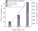
(a) Minimizing inputs with $4$ vertices per row.

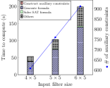
(b) Minimizing inputs with $5$ vertices per row.

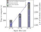
(c) Minimizing inputs with $6$ vertices per row.

Figure 8: A scalability test on the multi-outputting filter minimization problems. Inputs are $n\times m$ parameterized instances akin to Figure 7(a).

The time to construct the zipper constraints, prepare the formulas and the time used by the SAT solver were recorded. We also measured the number of zipper constraints found by our algorithm. Figure 8 summarizes the data for $(n,m)\in\{4,5,6\}\times\{4,5,6\}$. The result shows that about $70\text{\,}\mathrm{\char 37\relax}$ of the time is used in preparing the logical formula, with the SAT solver and construction of the zipper constraints accounting for only a very small fraction of time.

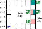
(a) A square environment for the robot to track the exits with the observation indicating its current row.

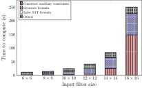
(b) Compute times to minimize filters with different sizes.

Figure 9: Navigating to exit a square environment with a row sensor.

In light of this, to further dissect the computational costs of different phases, we tested a robot in the square grid environment shown in Figure 9(a). The robot starts from the bottom left cell, and moves to some adjacent cell at each time step. The robot only receives observations indicating its row number at each step. We are interested in small filter allowing the robot to recognize whether it has reached a cell with an exit (at the inner side or outer side). States with both inner and outer exits have multiple outputs. To search for a minimal filter, we firstly start with deterministic input filters for a grid world with size $6\times 6$, $8\times 8$, $10\times 10$, $12\times 12$, $14\times 14$, $16\times 16$, and then minimize these filters. We collected the total time spent in different stages of filter minimization, including the construction of zipper constraints, SAT formula generation and resolution of SAT formula by the SAT solver. The results are summarized visually in Figure 9(b).

In this problem, the number of states in the input filter scales linearly with the size of the square. So does the minimal filter. But the particular problem has an important additional property: it represents a worst-case in a certain sense because there are no zipper constraints. We do not indicate this fact to the algorithm, so the construction of zipper constraints examines many cliques, determining that none apply. The results highlight that the construction of the zipper constraints quickly grows to overtake the time to generate the logical formula — even though, in this case, the zipper constraint set is empty.

The preceding hints toward our direction of current research: the construction of $\mathscr{Z}(F)$ by naïvely following Definition 14 is costly. And, though the SAT formula is polynomial in the size of the mcczc instance, that instance can be very large. On the other hand, the need for a zipper constraint can be detected when the output produced fails to be deterministic. Hence, our future work will look at how to generate these constraints lazily.

8 Conclusion

With an eye toward generalizing combinatorial filters, we introduced a new class of filter, the cover filters. Then, in order to reduce the state complexity of such filters, we re-examined earlier treatments of traditional filter minimization; this paper has shown some prior ideas to be mistaken. Building on these insights, we formulate the minimization problem via compatibility graphs, examining covers comprised of cliques formed thereon. We present an exact algorithm that generalizes from the traditional filter minimization problem to cover filters elegantly.

References

- [1] A. Censi, “A Class of Co-Design Problems With Cyclic Constraints and Their Solution,” IEEE Robotics and Automation Letters, vol. 2, no. 1, pp. 96–103, 2017.
- [2] A. Pervan and T. D. Murphey, “Low complexity control policy synthesis for embodied computation in synthetic cells,” in WAFR, Mérida, México, 2018.
- [3] F. Z. Saberifar, J. M. O’Kane, and D. A. Shell, “The hardness of minimizing design cost subject to planning problems,” in WAFR, Mérida, México, 2018.
- [4] S. M. LaValle, “Sensing and filtering: A fresh perspective based on preimages and information spaces,” Found. and Trends in Rob., vol. 1, no. 4, pp. 253–372, 2010.
- [5] J. M. O’Kane and D. A. Shell, “Concise planning and filtering: hardness and algorithms,” IEEE Transactions on Automation Science and Engineering, vol. 14, no. 4, pp. 1666–1681, 2017.
- [6] F. Z. Saberifar, S. Ghasemlou, J. M. O’Kane, and D. A. Shell, “Set-labelled filters and sensor transformations,” in Robotics: Science and Systems, 2016.
- [7] F. Z. Saberifar, S. Ghasemlou, D. A. Shell, and J. M. O’Kane, “Toward a language-theoretic foundation for planning and filtering,” International Journal of Robotics Research—WAFR’16 special issue, vol. 38, no. 2-3, pp. 236–259, 2019.
- [8] F. Z. Saberifar, A. Mohades, M. Razzazi, and J. M. O’Kane, “Combinatorial filter reduction: Special cases, approximation, and fixed-parameter tractability,” Journal of Computer and System Sciences, vol. 85, pp. 74–92, 2017.
- [9] H. Rahmani and J. M. O’Kane, “On the relationship between bisimulation and combinatorial filter reduction,” in Proceedings of IEEE International Conference on Robotics and Automation, Brisbane, Australia, 2018, pp. 7314–7321.
- [10] ——, “Integer linear programming formulations of the filter partitioning minimization problem,” Journal of Combinatorial Optimization, vol. 40, pp. 431–453, 2020.
- [11] Y. Zhang and D. A. Shell, “Cover Combinatorial Filters and their Minimization Problem (Extended Version),” arXiv preprint arXiv:2002.07153, 2020.
- [12] A. Nadel and V. Ryvchin, “Maple_LCM_Dist_ChronoBT: featuring chronological backtracking,” in Proc. of SAT Competition, 2018, pp. 29–30.
- [13] A. Ignatiev, A. Morgado, and J. Marques-Silva, “PySAT: A Python toolkit for prototyping with SAT oracles,” in SAT, 2018, pp. 428–437.