The existence of minimizers for an isoperimetric problem with Wasserstein penalty term in unbounded domains

Abstract

In this article, we consider the (double) minimization problem

$$\min\left\{P(E;\Omega)+\lambda W_{p}(\mathscr{L}^{d}\,\raisebox{-0.5468pt}{\reflectbox{\rotatebox[origin={br}]{-90.0}{$\lnot$}}}\,E,\mathscr{L}^{d}\,\raisebox{-0.5468pt}{\reflectbox{\rotatebox[origin={br}]{-90.0}{$\lnot$}}}\,F)\mathrel{\mathop{\ordinarycolon}}~{}E\subseteq\Omega,~{}F\subseteq\mathbb{R}^{d},~{}\mathinner{\!\left\lvert E\cap F\right\rvert}=0,~{}\mathinner{\!\left\lvert E\right\rvert}=\mathinner{\!\left\lvert F\right\rvert}=1\right\},$$

where $p\geqslant 1$, $\Omega$ is a (possibly unbounded) domain in $\mathbb{R}^{d}$, $P(E;\Omega)$ denotes the relative perimeter of $E$ in $\Omega$ and $W_{p}$ denotes the $p$-Wasserstein distance. When $\Omega$ is unbounded and $d\geqslant 3$, it is an open problem proposed by Buttazzo, Carlier and Laborde in the paper On the Wasserstein distance between mutually singular measures. We prove the existence of minimizers to this problem when $\frac{1}{p}+\frac{2}{d}>1$, $\Omega=\mathbb{R}^{d}$ and $\lambda$ is sufficiently small.

Keywords: isoperimetric problem, Wasserstein distance, quasi-perimeter, unbounded domains, volume constraints.

2010 Mathematics Subject Classifications: 49J45, 49Q20, 49Q05, 49J20.

1 Introduction

In this paper, we consider an open question left by Buttazzo, Carlier and Laborde in [BCL17]. Let $\Omega$ denote a (possibly unbounded) open domain in $\mathbb{R}^{d}$ with volume $\mathinner{\!\left\lvert\Omega\right\rvert}>1$. For $\lambda\geqslant 0$ and $p\geqslant 1$, authors of [BCL17] consider the following (double) minimization problem:

$$\min\left\{P(E;\Omega)+\lambda W_{p}(\mathscr{L}^{d}\,\raisebox{-0.5468pt}{\reflectbox{\rotatebox[origin={br}]{-90.0}{$\lnot$}}}\,E,\mathscr{L}^{d}\,\raisebox{-0.5468pt}{\reflectbox{\rotatebox[origin={br}]{-90.0}{$\lnot$}}}\,F)\mathrel{\mathop{\ordinarycolon}}~{}E\subseteq\Omega,~{}F\subseteq\mathbb{R}^{d},~{}\mathinner{\!\left\lvert E\cap F\right\rvert}=0,~{}\mathinner{\!\left\lvert E\right\rvert}=\mathinner{\!\left\lvert F\right\rvert}=1\right\}$$ (1.1)

where $P(E;\Omega)$ denotes the relative perimeter of $E$ in $\Omega$ ([Mag12]) and $W_{p}$ denotes the $p$-Wasserstein distance ([Vil03]) between probability measures.

As studied in [PR09, LPR14], this type of problem arises from some biological models of bi-layer membranes. To study such an isoperimetric problem with Wasserstein penalty term, to our best knowledge, most literature assume that $\Omega$ is bounded and $F$ is given. For instance, to model materials cracking problem, the first author in [Xia05] studies the existence and regularity when the second term is replaced by $\lambda W_{p}^{p}(\mathscr{L}^{d}\,\raisebox{-0.5468pt}{\reflectbox{\rotatebox[origin={br}]{-90.0}{$\lnot$}}}\,E,\sigma\mathscr{L}^{d}\,\raisebox{-0.5468pt}{\reflectbox{\rotatebox[origin={br}]{-90.0}{$\lnot$}}}\,\Omega)$, where $\Omega$ is bounded and $\mathinner{\!\left\lvert E\right\rvert}=\sigma\mathinner{\!\left\lvert\Omega\right\rvert}$. Milakis in [Mil06] studies an analogous problem for $W_{2}^{2}(\mathscr{L}^{d}\,\raisebox{-0.5468pt}{\reflectbox{\rotatebox[origin={br}]{-90.0}{$\lnot$}}}\,E,\mathscr{L}^{d}\,\raisebox{-0.5468pt}{\reflectbox{\rotatebox[origin={br}]{-90.0}{$\lnot$}}}\,F)$ as the second term when $\Omega$ is a bounded smooth domain and $F$ is given. In other scenarios, for fixed $F$, if one replaces the perimeter term by some functional on $E$ and adopts $W_{2}^{2}(\mathscr{L}^{d}\,\raisebox{-0.5468pt}{\reflectbox{\rotatebox[origin={br}]{-90.0}{$\lnot$}}}\,E,\mathscr{L}^{d}\,\raisebox{-0.5468pt}{\reflectbox{\rotatebox[origin={br}]{-90.0}{$\lnot$}}}\,F)$, such a variational problem corresponds to the Jordan-Kinderlehrer-Otto (JKO) scheme ([JKO98]), which can be regarded as a gradient flow under Wasserstein metric (see the review paper [San17]). This leads to many interesting problems and applications (see [DPMSV16, San18, DMS19]). When $\Omega$ is unbounded, besides the classical Euclidean isoperimetric problem (see [Mor96]) and the founding work by Almgren in [Alm76] on minimizing clusters problem, Knüpfer and Muratov in [KM13, KM14] study an isopermetric problem with a non-Wasserstein term. The penalty term there are generated by a kernel given by an inverse power of the distance. Other related work might be found in [FFM⁺15].

In [BCL17] Buttazzo et al. prove the existence of minimizers to (1.1) for the following cases when $\lambda>0$:

• For any $d$, when $\Omega$ is bounded, the minimization problem (1.1) admits a solution.

• For $d=2$ and $\Omega=\mathbb{R}^{2}$, the minimization problem (1.1) admits a solution.

• For $d=1$, a solution can be constructed by disjoint equal sub-intervals, whose number depends on $\lambda$.

Their proof for the case $d=2$ and $\Omega=\mathbb{R}^{2}$ relies on the fact that for a connected set, its diameter is bounded by its perimeter, which only holds for dimension two. Therefore the existence to such a minimization problem is still open for a unbounded domain $\Omega$ of dimension more than two.

In this article, we adopt a new approach that is valid for every dimension $d$. It provides the existence result in every dimension for small $\lambda$.

Theorem 1.1.

Suppose $p\geqslant 1$, $d\geqslant 1$ with $\frac{1}{p}+\frac{2}{d}>1$ and $\Omega=\mathbb{R}^{d}$, there exists $\lambda_{0}=\lambda_{0}(d,p)>0$, such that for any $0<\lambda\leqslant\lambda_{0}$, the minimization problem

$$\min\left\{P(E)+\lambda W_{p}(\mathscr{L}^{d}\,\raisebox{-0.5468pt}{\reflectbox{\rotatebox[origin={br}]{-90.0}{$\lnot$}}}\,E,\mathscr{L}^{d}\,\raisebox{-0.5468pt}{\reflectbox{\rotatebox[origin={br}]{-90.0}{$\lnot$}}}\,F)\mathrel{\mathop{\ordinarycolon}}~{}E,F\subseteq\mathbb{R}^{d},~{}\mathinner{\!\left\lvert E\cap F\right\rvert}=0,~{}\mathinner{\!\left\lvert E\right\rvert}=\mathinner{\!\left\lvert F\right\rvert}=1\right\}$$ (1.2)

admits a solution.

For $d\geqslant 3$ and $\Omega=\mathbb{R}^{d}$, the main difficulty is that we only have compactness of sets of locally finite perimeter. As a consequence, the limit set of any minimizing sequence with respect to convergence in measure may not satisfy the volume constraint. To overcome this obstacle, we adopt the following strategy:

• Equivalent formulation in a volume parameter $m$. To normalize the parameter $\lambda$ in the problem (1.2), we apply scaling arguments and obtain an equivalent formulation in the problem (3.8) with a volume parameter $\mathinner{\!\left\lvert E\right\rvert}=m$.

• Existence of a minimizing sequence of bounded sets. We prove in Theorem 5.1 that there exists a minimizing sequence of bounded sets to the problem (3.8). In our proof, we use a “covering-packing” technique: We first cover the majority of the set $E$ by a prescribed number of balls with same radius in Proposition 5.3. Here we use the so-called Nucleation Lemma in [Mag12], which is a tool from Almgren’s seminal paper [Alm76] for minimizing clusters problem. Then we pack all balls into a ball of prescribed radius in Theorem 5.4. Applying this “covering-packing” technique to any given minimizing sequence, we obtain an alternative minimizing sequence of bounded sets as desired. Now, by using the known result for $\mathcal{W}_{p}(E)\vcentcolon=\min_{F}W_{p}(E,F)$ on any bounded set $E$, we express the double minimizing problem (3.8) into an equivalent single minimizing problem (5.5): $\textrm{Minimize~{}}P(E)+\mathcal{W}_{p}(E)$ among all bounded sets $E$ with $\mathinner{\!\left\lvert E\right\rvert}=m$.

• Existence of a minimizing sequence of uniformly bounded sets for small volume. To apply the direct method of calculus of variations, we further require uniform boundedness. When the volume is small, in Theorem 6.3 we are able to find a minimizing sequence of uniformly bounded sets to the problem (5.5), through a non-optimality criterion in Proposition 6.2. Our work is inspired by the seminal work of Knüpfer and Muratov in [KM14] for an isoperimetric problem with a competing non-local term in unbounded domains.

Remark.

It is interesting to compare the non-local functional $V(E)=\int_{E}\int_{E}\frac{1}{\mathinner{\!\left\lvert x-y\right\rvert}^{\alpha}}\mathop{}\!\mathrm{d}{x}\mathop{}\!\mathrm{d}{y}$ for $\alpha\in(0,d)$ in [KM14] with the non-local Wasserstein term $\mathcal{W}_{p}(E)=\min_{F}W_{p}(E,F)$. Both non-local terms behave like repulsive effects with respect to the set itself. The non-local term in [KM14], among which the Coulombic repulsion is a special case, is in an exact integral form. Thus it has a natural advantage to compare the functional between different sets. In opposite, the Wasserstein term consists of a minimizing process. It requires to minimize among all disjoint sets of equal volume, and to minimize among all admissible transport plans, which bring novel obstacles.

The remaining of the paper is organized as follows: in Section 2 we introduce the notations throughout the paper. In Section 3 we recall some basic definitions in geometric measure theory, with an emphasis on the theory about sets of finite perimeter and optimal transport theory. In Section 3.3 we reformulate the problem (1.2) into the problem (3.8). In Section 4, we introduce the Wasserstein functional $\mathcal{W}_{p}(E)$ on any bounded Lebesgue measurable set $E$ and study its properties. In Section 5, we prove the existence of a minimizing sequence of bounded sets to the problem (3.8), by which we reformulate again the problem (3.8) into the problem (5.5). In Section 6, for small volume sets, we prove the existence of a minimizing sequence of uniformly bounded sets, and use it to prove the existence of minimizers for the problem (5.5).

2 Notations

We use the following notations below throughout the paper.

$B(x,r)$ or $B_{r}(x)$	Open $d$-ball centered at $x$ of radius $r$ in $\mathbb{R}^{d}$.
$\omega_{d}$	the volume of unit $d-$ball.
$\ell_{d}=(\omega_{d})^{-1/d}$	The radius of $d-$ball of volume 1.
$C_{1}\sqcup C_{2}$	Disjoint union of sets $C_{1}$ and $C_{2}$.
$C_{1}\Delta C_{2}=(C_{1}\setminus C_{2})\cup(C_{2}\setminus C_{1})$	Symmetric difference of sets $C_{1}$ and $C_{2}$.
$rE=\left\{rx\mathrel{\mathop{\ordinarycolon}}x\in E\right\}$	Re-scaling of a set $E$.
$E+a=\left\{x+b\mathrel{\mathop{\ordinarycolon}}x\in E\right\}$	Translation of a set $E$.
$\mathbbm{1}_{E}$	The characteristic function of set $E$.
$\mathscr{L}^{d}$ or $\mathop{}\!\mathrm{d}{x}$	Lebesgue measure.
$\mathscr{L}^{d}\,\raisebox{-0.5468pt}{\reflectbox{\rotatebox[origin={br}]{-90.0}{$\lnot$}}}\,E$	$d-$Lebesgue measure restricted on a set $E$.
$\mathinner{\!\left\lvert E\right\rvert}=\mathscr{L}^{d}(E)$	Volume ($d-$Lebesgue measure) of a set $E$.
$\Phi_{\#}\mu$	Push-forward of measure $\mu$ by the mapping $\Phi$.
$\displaystyle\textrm{dist}(x,E)=\inf_{y\in E}\textrm{dist}(x,y)$	Distance between a point $x$ and a set $E$ in $\mathbb{R}^{d}$.
$\mathcal{P}_{c}(\mathbb{R}^{d})$	the class of all probability measures on $\mathbb{R}^{d}$ with compact support.
$\mu\perp\nu$	measures $\mu$ and $\nu$ are mutually singular.

3 Preliminaries

In this section, we first recall related concepts in geometric measure theory with an emphasis on sets of finite perimeter [Mag12] and optimal transport theory [Vil03, Vil09].

3.1 Sets of finite perimeter

In this subsection, we closely follow Maggi’s book [Mag12].

Definition 1 (Set of finite perimeter).

We say that a Lebesgue measurable set $E\subseteq\mathbb{R}^{d}$ is a set of locally finite perimeter if for every compact set $K\subseteq\mathbb{R}^{d}$ we have

$$\sup\left\{\int_{E}\textrm{div~{}}\phi(x)\mathop{}\!\mathrm{d}{x}\mathrel{\mathop{\ordinarycolon}}\phi\in C_{c}^{1}(\mathbb{R}^{d};\mathbb{R}^{d}),\textrm{spt~{}}\phi\subseteq K,\sup_{\mathbb{R}^{d}}\mathinner{\!\left\lvert\phi\right\rvert}\leqslant 1\right\}<\infty.$$

If the above quantity is bounded independently of $K$, then we say $E$ is a set of finite perimeter.

If $E$ is a set of locally finite perimeter, then there exists a $\mathbb{R}^{d}-$valued Radon measure $\mu_{E}$, called the distributional derivative of set $E$, such that

$$\int_{E}\textrm{div~{}}\phi(x)\mathop{}\!\mathrm{d}{x}=\int_{\mathbb{R}^{d}}\phi\cdot\mathop{}\!\mathrm{d}{\mu_{E}},\qquad\forall\phi\in C_{c}^{1}(\mathbb{R}^{d};\mathbb{R}^{d}).$$

The perimeter of $E$ in $\Omega$, denoted by $P(E;\Omega)$, is the variation of $\mu_{E}$ in $\Omega$, i.e.,

$$P(E;\Omega)\vcentcolon=\mathinner{\!\left\lvert\mu_{E}\right\rvert}(\Omega).$$

When $\Omega=\mathbb{R}^{d}$, we adopt $P(E)$ for simplicity.

Definition 2 (Convergence in measure).

Given a sequence $\{E_{n}\}$ of Lebesgue measurable sets and $E$ in $\mathbb{R}^{d}$, we say that $E_{n}$ locally converges to $E$, denoted by $E_{n}\xrightarrow[]{\textrm{loc}}E$, if

$$\lim_{n\to\infty}\mathinner{\!\left\lvert K\cap(E\Delta E_{n})\right\rvert}=0,\qquad\qquad\forall K\subseteq\mathbb{R}^{d}\textrm{~{}compact}.$$

We say $E_{n}$ converges to $E$, denoted by $E_{n}\to E$, if

$$\lim_{n\to\infty}\mathinner{\!\left\lvert E\Delta E_{n}\right\rvert}=0.$$

Proposition 3.1 (Lower semi-continuity of perimeter).

If $\{E_{n}\}$ is a sequence of sets of locally finite perimeter in $\mathbb{R}^{d}$ with

$$E_{n}\xrightarrow[]{\textrm{loc}}E,\qquad\limsup_{n\to\infty}P(E_{n};K)<\infty,$$

for every compact set $K$ in $\mathbb{R}^{d}$, then $E$ is of locally finite perimeter in $\mathbb{R}^{d}$, $\mu_{E_{n}}\xrightharpoonup{*}\mu_{E}$, and for every open set $\Omega\subseteq\mathbb{R}^{d}$, we have

$$P(E;\Omega)\leqslant\liminf_{n\to\infty}P(E_{n};\Omega).$$

Proposition 3.2 (Compactness of uniformly bounded sets of finite perimeter).

If $r>0$ and $\{E_{n}\}$ are sets of finite perimeter in $\mathbb{R}^{d}$, with

$$\sup_{n}P(E_{n})<\infty,\qquad\mathrm{and}\qquad E_{n}\subseteq B_{r},\quad\forall n.$$

Then there exists a set $E$ of finite perimeter in $\mathbb{R}^{d}$, such that up to extracting a subsequence (still denoted by $E_{n}$):

$$E_{n}\to E,\qquad\mu_{E_{n}}\xrightharpoonup{*}\mu_{E},\qquad E\subseteq B_{r}.$$

Corollary 3.3 (Local compactness of sets of locally finite perimeter).

If $\{E_{n}\}$ are sets of locally finite perimeter in $\mathbb{R}^{d}$ with

$$\sup_{h}P(E_{h};B_{r})<\infty,\qquad\forall r>0.$$

Then there exists a set $E$ of locally finite perimeter, such that up to extracting a subsequence (still denoted by $B_{n}$):

$$E_{n}\xrightarrow[]{\textrm{loc}}E,\qquad\mu_{E_{n}}\xrightharpoonup{*}\mu_{E}.$$

As in [FMP10], the isoperimetric deficit of a set of finite perimeter $E\subseteq\mathbb{R}^{d}$ is defined by

$$D(E)\vcentcolon=\frac{P(E)-P(B_{r})}{P(B_{r})},$$ (3.1)

where $B_{r}$ is a $d-$ball with $\mathinner{\!\left\lvert B_{r}\right\rvert}=\mathinner{\!\left\lvert E\right\rvert}$.

The Fraenkel asymmetry of two measurable sets $E_{1}$ and $E_{2}$ with $\mathinner{\!\left\lvert E_{1}\right\rvert}=\mathinner{\!\left\lvert E_{2}\right\rvert}$ is defined by

$$\Delta(E_{1},E_{2})\vcentcolon=\min_{x\in\mathbb{R}^{d}}\frac{\mathinner{\!\left\lvert E_{1}\Delta(E_{2}+x)\right\rvert}}{\mathinner{\!\left\lvert E_{1}\right\rvert}},$$ (3.2)

where $E_{2}+x=\left\{y+x\mathrel{\mathop{\ordinarycolon}}y\in E_{2}\right\}$.

Theorem 3.4 ([FMP10], Quantitative isoperimetric inequality).

There exists a constant $C(d)$ such that for any set $F\subseteq\mathbb{R}^{d}$ of finite perimeter, we have

$$\Delta(E,B_{r})\leqslant C(d)\sqrt{D(E)},$$ (3.3)

where $B_{r}$ is a $d-$ball with $\mathinner{\!\left\lvert B_{r}\right\rvert}=\mathinner{\!\left\lvert E\right\rvert}$.

3.2 Optimal transport theory

Definition 3 (Wasserstein distance).

Let $\mathcal{P}_{p}(\mathbb{R}^{d})\vcentcolon=\left\{\mu\in\mathcal{P}(\mathbb{R}^{d})\mathrel{\mathop{\ordinarycolon}}\int_{\mathbb{R}^{d}}\mathinner{\!\left\lvert x-x_{0}\right\rvert}^{p}\mathop{}\!\mathrm{d}{\mu}(x)<+\infty\right\}$ for some point $x_{0}\in\mathbb{R}^{d}$. For $\mu,\nu\in\mathcal{P}_{p}(\mathbb{R}^{d})$, the $p$-Wasserstein distance between $\mu$ and $\nu$ is given by

$$W_{p}(\mu,\nu)\vcentcolon=\inf_{\gamma\in\Gamma(\mu,\nu)}\left(\int_{\mathbb{R}^{d}\times\mathbb{R}^{d}}\mathinner{\!\left\lvert x-y\right\rvert}^{p}\mathop{}\!\mathrm{d}{\gamma}(x,y)\right)^{1/p},$$ (3.4)

where $\Gamma(\mu,\nu)$ is the collection of the so-called transport plans from $\mu$ to $\nu$, defined by

$$\Gamma(\mu,\nu)\vcentcolon=\left\{\gamma\in P(\mathbb{R}^{d}\times\mathbb{R}^{d})\mathrel{\mathop{\ordinarycolon}}(\pi_{x})_{\#}\gamma=\mu,(\pi_{y})_{\#}\gamma=\nu\right\},$$ (3.5)

where $\pi_{x},\pi_{y}$ denote the projection from $\mathbb{R}^{d}\times\mathbb{R}^{d}$ onto each marginal space.

With a slight abuse of notation, given two Lebesgue measurable sets $E,F$ with $\mathinner{\!\left\lvert E\right\rvert}=\mathinner{\!\left\lvert F\right\rvert}=m$, $W_{p}(E,F)$ is given by

$$W_{p}(E,F)\vcentcolon=W_{p}(\mathscr{L}^{d}\,\raisebox{-0.5468pt}{\reflectbox{\rotatebox[origin={br}]{-90.0}{$\lnot$}}}\,E,\mathscr{L}^{d}\,\raisebox{-0.5468pt}{\reflectbox{\rotatebox[origin={br}]{-90.0}{$\lnot$}}}\,F)=m^{\frac{1}{p}+\frac{1}{d}}W_{p}(\mathscr{L}^{d}\,\raisebox{-0.5468pt}{\reflectbox{\rotatebox[origin={br}]{-90.0}{$\lnot$}}}\,(m^{-1/d}E),\mathscr{L}^{d}\,\raisebox{-0.5468pt}{\reflectbox{\rotatebox[origin={br}]{-90.0}{$\lnot$}}}\,(m^{-1/d}F)).$$

When $E,F$ are bounded sets of equal volume in $\mathbb{R}^{d}$ and $p\in[1,\infty)$, it is well-known ([Bre91], [GM96], [Amb03], and see also Chapter 1 and Chapter 3 in [San15]) that there exists an optimal transport map $\Phi$ that transports $E$ to $F$, in the sense that $\Phi_{\#}(\mathscr{L}^{d}\,\raisebox{-0.5468pt}{\reflectbox{\rotatebox[origin={br}]{-90.0}{$\lnot$}}}\,E)=\mathscr{L}^{d}\,\raisebox{-0.5468pt}{\reflectbox{\rotatebox[origin={br}]{-90.0}{$\lnot$}}}\,F$ and

$$W_{p}(E,F)=\left(\int_{E}\mathinner{\!\left\lvert x-\Phi(x)\right\rvert}^{p}\mathop{}\!\mathrm{d}{x}\right)^{1/p}.$$

3.3 Equivalent formulation of problem $\eqref{eq: minEset}$

For convenience sake, we consider an equivalent formulation of problem (1.2) by using scaling arguments.

For any $m>0$, denote

$$\mathcal{F}_{m}\mathrel{\mathop{\ordinarycolon}}=\left\{(E,F)\mathrel{\mathop{\ordinarycolon}}~{}E,F\subseteq\mathbb{R}^{d},~{}\mathinner{\!\left\lvert E\cap F\right\rvert}=0,~{}\mathinner{\!\left\lvert E\right\rvert}=\mathinner{\!\left\lvert F\right\rvert}=m\right\}.$$

Then the minimization problem (1.2) becomes

$$\text{ Minimize }\qquad P(E)+\lambda W_{p}(E,F)\qquad\text{ among all }(E,F)\in\mathcal{F}_{1}.$$ (3.6)

Note that for any $(E,F)\in\mathcal{F}_{1}$ and $r>0$, by the scaling argument, it follows that $(rE,rF)\in\mathcal{F}_{m}$ for $m=r^{d}$ with

$$P(rE)=r^{d-1}P(E)\quad\textrm{and}\quad W_{p}(rE,rF)=r^{1+\frac{d}{p}}W_{p}(E,F).$$ (3.7)

Now, by setting $m$ to be the number such that

$$\lambda=m^{\frac{1}{p}+\frac{2}{d}-1}\quad\textrm{and~{}let}\quad r=m^{\frac{1}{d}},$$

we have

$$P(rE)+W_{p}(rE,rF)= r^{d-1}P(E)+r^{1+\frac{d}{p}}W_{p}(E,F)$$

$$= r^{d-1}\left(P(E)+r^{d(\frac{2}{d}+\frac{1}{p}-1)}W_{p}(E,F)\right)$$

$$= r^{d-1}\left(P(E)+\lambda W_{p}(E,F)\right).$$

This gives an equivalent formulation of problem (3.6): For any $m\geqslant 0$,

$$\text{ Minimize }\qquad P(E)+W_{p}(E,F)\qquad\textrm{among~{}all~{}}(E,F)\in\mathcal{F}_{m}.$$ (3.8)

Any solution $(E,F)\in\mathcal{F}_{m}$ to problem (3.8) corresponds to a solution $(m^{-\frac{1}{d}}E,m^{-\frac{1}{d}}F)\in\mathcal{F}_{1}$ to problem (3.6) (i.e. problem (1.2)) for

$$\lambda=m^{{}^{\frac{1}{p}+\frac{2}{d}-1}}$$ (3.9)

and

$$P(m^{-\frac{1}{d}}E)+\lambda W_{p}(m^{-\frac{1}{d}}E,m^{-\frac{1}{d}}F)=m^{\frac{1}{d}-1}\left(P(E)+W_{p}(E,F)\right).$$

As a result, to prove Theorem 1.1, it is equivalent to prove the following theorem:

Theorem 3.5.

For $\frac{1}{p}+\frac{2}{d}>1$ and $\Omega=\mathbb{R}^{d}$, there exists $m_{0}=m_{0}(d,p)>0$, such that for any $0<m\leqslant m_{0}$, the minimization problem

$$\min\left\{P(E)+W_{p}(E,F)\mathrel{\mathop{\ordinarycolon}}(E,F)\in\mathcal{F}_{m}\right\}$$ (3.10)

admits a solution.

4 The Wasserstein functional on bounded sets

Lemma 4.1.

For any bounded Lebesgue measurable set $E\subseteq\mathbb{R}^{d}$, there exists a set $F$ such that $(E,F)\in\mathcal{F}_{m}$ with $m\vcentcolon=\mathinner{\!\left\lvert E\right\rvert}<\infty$, and

$$W_{p}(E,F)=\min\left\{W_{p}(E,\widetilde{F})\mathrel{\mathop{\ordinarycolon}}(E,\widetilde{F})\in\mathcal{F}_{m}\right\}.$$

Proof.

Without loss of generality, we may assume that $m=1$ by applying the scaling argument (3.7). Then the existence of a minimizer $F$ follows from Theorem 3.10 in [BCL17] (as re-stated below ) with $\mu=\mathscr{L}^{d}\,\raisebox{-0.5468pt}{\reflectbox{\rotatebox[origin={br}]{-90.0}{$\lnot$}}}\,E$, $\phi\equiv 1$ and the observation that $\mathscr{L}^{d}\,\raisebox{-0.5468pt}{\reflectbox{\rotatebox[origin={br}]{-90.0}{$\lnot$}}}\,\widetilde{F}\in\mathcal{A}_{\phi}$ whenever $(E,\widetilde{F})\in\mathcal{F}_{m}$. ∎

Here, we restate Theorem 3.10 in [BCL17] with minor modifications in notations:

Theorem 4.2 (Theorem 3.10 in [BCL17]).

For any $\mu\in\mathcal{P}_{c}(\mathbb{R}^{d})$, given a nonnegative integrable function $\phi(x)$ on $\mathbb{R}^{d}$ with $\int_{\mathbb{R}^{d}\setminus\textrm{supp}(\mu)}\phi(x)\mathop{}\!\mathrm{d}{x}>1$, let $\mathcal{A_{\phi}}$ denote a collection of measures, defined by

$$\mathcal{A}_{\phi}=\left\{\nu\in\mathcal{P}_{c}\mathrel{\mathop{\ordinarycolon}}\nu\perp\mu,\frac{\mathop{}\!\mathrm{d}{\nu}}{\mathop{}\!\mathrm{d}{x}}\leqslant\phi\right\}.$$

Then there exists a set $A$ such that the measure $\nu_{0}\mathrel{\mathop{\ordinarycolon}}=\phi\mathscr{L}^{d}\,\raisebox{-0.5468pt}{\reflectbox{\rotatebox[origin={br}]{-90.0}{$\lnot$}}}\,{A}$ is in $\mathcal{A}_{\phi}$ and satisfies

$$W_{p}(\mu,\nu_{0})=\min_{\nu\in A_{\phi}}W_{p}(\mu,\nu).$$

Definition 4.

For any bounded Lebesgue measurable set $E\subseteq\mathbb{R}^{d}$ and $p\geqslant 1$, let $m\vcentcolon=\mathinner{\!\left\lvert E\right\rvert}$ and define the Wasserstein functional on $E$ by

$$\mathcal{W}_{p}(E)\mathrel{\mathop{\ordinarycolon}}=\min\{W_{p}(E,\widetilde{F})\mathrel{\mathop{\ordinarycolon}}~{}(E,\widetilde{F})\in\mathcal{F}_{m}\}.$$ (4.1)

By the scaling argument (3.7), it follows that

$$\mathcal{W}_{p}(rE)=r^{1+\frac{d}{p}}\mathcal{W}_{p}(E).$$ (4.2)

Lemma 4.3.

For any bounded Lebesgue measurable set $E\subseteq\mathbb{R}^{d}$ and $p\geqslant 1$, let $F$ denote a $\mathcal{W}_{p}$-minimizer of $E$ and $\Phi$ denote an optimal transport map that transports $E$ to $F$. Then there is a constant $C_{0}(d)=(3^{1/d}+2)\ell_{d}$ such that

1. For a.e. $x\in E$

   $$\mathinner{\!\left\lvert\Phi(x)-x\right\rvert}\leqslant C_{0}(d)\mathinner{\!\left\lvert E\right\rvert}^{1/d}.$$ (4.3)

2. $$\mathcal{W}_{p}(E)\leqslant C_{0}(d)\mathinner{\!\left\lvert E\right\rvert}^{\frac{1}{p}+\frac{1}{d}}.$$ (4.4)

3. $$\mathinner{\!\left\lvert F\setminus\left\{y\in\mathbb{R}^{d}\mathrel{\mathop{\ordinarycolon}}\textrm{dist}(y,E)\leqslant C_{0}(d)\mathinner{\!\left\lvert E\right\rvert}^{1/d}\right\}\right\rvert}=0.$$ (4.5)

Proof.

Without loss of generality, by (4.2) we may assume that $\mathinner{\!\left\lvert E\right\rvert}=1$.

Let $K=\left\{x\in E\mathrel{\mathop{\ordinarycolon}}\mathinner{\!\left\lvert\Phi(x)-x\right\rvert}>(3^{1/d}+2)\ell_{d}\right\}$. We want to show that $\mathinner{\!\left\lvert K\right\rvert}=0$. Indeed, assume $\mathinner{\!\left\lvert K\right\rvert}>0$, then there exists $x_{0}\in K$ such that for some $0<r\leqslant\ell_{d}$, we have $\mathinner{\!\left\lvert K\cap B(x_{0},r)\right\rvert}>0$.

Since $\mathinner{\!\left\lvert K\cap B(x_{0},r)\right\rvert}\leqslant\mathinner{\!\left\lvert B(x_{0},r)\right\rvert}\leqslant\mathinner{\!\left\lvert B(x_{0},\ell_{d})\right\rvert}=1$ and

$$\mathinner{\!\left\lvert B(x_{0},3^{1/d}\ell_{0})\setminus(E\cup F)\right\rvert}\geqslant\mathinner{\!\left\lvert B(x_{0},3^{1/d}\ell_{d})\right\rvert}-\mathinner{\!\left\lvert E\right\rvert}-\mathinner{\!\left\lvert F\right\rvert}=3-1-1=1,$$

there exists a subset $H\subseteq B(x_{0},3^{1/d}\ell_{d})\setminus(E\cup F)$ with $\mathinner{\!\left\lvert H\right\rvert}=\mathinner{\!\left\lvert K\cap B(x_{0},r)\right\rvert}$ and $\mathinner{\!\left\lvert H\cap(K\cap B(x_{0},r))\right\rvert}=0$. Let $\Psi$ be an optimal transport map from $K\cap B(x_{0},r)$ to $H$.

Now we construct a new mapping:

$$\bar{\Phi}(x)=\left\{\begin{aligned} &\Phi(x)\qquad x\in E\setminus(K\cap B(x_{0},r));\\ &\Psi(x)\qquad x\in K\cap B(x_{0},r).\end{aligned}\right.$$

By our construction, $\mathinner{\!\left\lvert\bar{\Phi}(E)\cap E\right\rvert}=0$. Note that for

$$\mathinner{\!\left\lvert\bar{\Phi}(E)\right\rvert}=\mathinner{\!\left\lvert\Psi(K\cap B(x_{0},r))\right\rvert}+\mathinner{\!\left\lvert\Phi(E\setminus(K\cap B(x_{0},r)))\right\rvert}=\mathinner{\!\left\lvert K\cap B(x_{0},r)\right\rvert}+\mathinner{\!\left\lvert E\setminus(K\cap B(x_{0},r))\right\rvert}=\mathinner{\!\left\lvert E\right\rvert},$$

Thus $(E,\bar{\Phi}(E))\in\mathcal{F}_{1}$. Moreover, for a.e. $x\in K\cap B(x_{0},r)$,

$$\mathinner{\!\left\lvert\Psi(x)-x\right\rvert} \leqslant\mathinner{\!\left\lvert\Psi(x)-x_{0}\right\rvert}+\mathinner{\!\left\lvert x_{0}-x\right\rvert}$$

$$\leqslant 3^{1/d}\ell_{d}+r\leqslant(3^{1/d}+1)\ell_{d}$$

$$<\mathinner{\!\left\lvert\Phi(x)-x\right\rvert}-\ell_{d}.$$

Thus, since $\mathinner{\!\left\lvert K\cap B(x_{0},r)\right\rvert}>0$, it holds that

$$\int_{E}\mathinner{\!\left\lvert\bar{\Phi}(x)-x\right\rvert}^{p}\mathop{}\!\mathrm{d}{x}-\int_{E}\mathinner{\!\left\lvert\Phi(x)-x\right\rvert}^{p}\mathop{}\!\mathrm{d}{x}=\int_{K\cap B(x_{0},r)}\mathinner{\!\left\lvert\Psi(x)-x\right\rvert}^{p}\mathop{}\!\mathrm{d}{x}-\int_{K\cap B(x_{0},r)}\mathinner{\!\left\lvert\Phi(x)-x\right\rvert}^{p}\mathop{}\!\mathrm{d}{x}<0.$$

This shows that

$$W_{p}(E,\bar{\Phi}(E))<W_{p}(E,F),$$

a contradiction with $F$ being the $\mathcal{W}_{p}$-minimizer of $E$.

Hence for a.e. $x\in E$,

$$\mathinner{\!\left\lvert\Phi(x)-x\right\rvert}\leqslant C_{0}(d)\mathinner{\!\left\lvert E\right\rvert}^{1/d}.$$

As a result,

$$\mathcal{W}_{p}(E)=W_{p}(E,F)=\left(\int_{E}\mathinner{\!\left\lvert\Phi(x)-x\right\rvert}^{p}\mathop{}\!\mathrm{d}{x}\right)^{1/p}\leqslant C_{0}(d)\mathinner{\!\left\lvert E\right\rvert}^{\frac{1}{p}+\frac{1}{d}},$$

and

$$\mathinner{\!\left\lvert F\setminus\left\{y\in\mathbb{R}^{d}\mathrel{\mathop{\ordinarycolon}}\textrm{dist}(y,E)\leqslant C_{0}(d)\mathinner{\!\left\lvert E\right\rvert}^{1/d}\right\}\right\rvert}=0.$$

∎

Lemma 4.4 (Lower semi-continuity of $\mathcal{W}_{p}$).

Suppose $\{E_{n}\}$ is any sequence of sets of finite perimeter in $\mathbb{R}^{d}$ with

$$\sup_{n}P(E_{n})<\infty\qquad\mathrm{and}\qquad E_{n}\subseteq B_{R}$$

for each $n$ and some $R>0$. If $E_{n}$ converges to $E$, then we have

$$\mathcal{W}_{p}(E)\leqslant\liminf_{n\to\infty}\mathcal{W}_{p}(E_{n}).$$

Proof.

By the definition of $\liminf$, up to extracting a subsequence of $\left\{E_{n}\right\}$ if necessary (still denoted by $\left\{E_{n}\right\}$), we may assume that

$$\lim_{n\to\infty}\mathcal{W}_{p}(E_{n})=\liminf_{n\to\infty}W_{p}(E_{n}).$$

Let $F_{n}$ denote corresponding $\mathcal{W}_{p}$-minimizer of $E_{n}$ such that $\mathcal{W}_{p}(E_{n})=W_{p}(E_{n},F_{n})$. By Theorem 3.13 and Remark 3.14 in [BCL17], $F_{n}$ is also a set of finite perimeter with a uniform bound on its perimeter. Furthermore, by (4.5) in Lemma 4.3, $\left\{F_{n}\right\}$ are contained in $B_{R^{\prime}}$ for $R^{\prime}=R+C_{0}(d)\mathinner{\!\left\lvert E\right\rvert}^{1/d}$. Thanks to the compactness of sets of finite perimeter, there exists a set $F$ of finite perimeter in $B_{R^{\prime}}$ and a subsequence $\{F_{n_{k}}\}$ such that $F_{n_{k}}\to F$.

Since $W_{p}$ is lower semi-continuous with respect to weak convergence, we have

$$W_{p}(E,F)\leqslant\liminf_{n\to\infty}W_{p}(E_{n_{k}},F_{n_{k}}).$$

For any $k$,

$$E\cap F\subseteq(E\setminus E_{n_{k}})\cup(F\setminus F_{n_{k}})\cup(E_{n_{k}}\cap F_{n_{k}}),$$

which yields that $\mathinner{\!\left\lvert E\cap F\right\rvert}=0$. Therefore,

$$\mathcal{W}_{p}(E)\leqslant W_{p}(E,F)\leqslant\liminf_{k\to\infty}W_{p}(E_{n_{k}},F_{n_{k}})=\liminf_{k\to\infty}\mathcal{W}_{p}(E_{n_{k}})=\lim_{n\to\infty}\mathcal{W}_{p}(E_{n})=\liminf_{n\to\infty}W_{p}(E_{n}).$$

∎

5 Existence of minimizing sequence of bounded sets

In this section, we will prove the following theorem:

Theorem 5.1.

There exists a minimizing sequence of bounded sets to problem (3.8).

We will show that for any minimizing sequence $(E_{n},F_{n})$ to (3.8), there is an alternative minimizing sequence $(\widetilde{E_{n}},\widetilde{F_{n}})$ of bounded sets to (3.8).

Remark.

Here, $(\widetilde{E_{n}},\widetilde{F_{n}})$ is not necessarily uniformly bounded.

We first start with an important lemma, originating from Almgren’s breakthrough work in [Alm76], and rephrased in [Mag12]:

Lemma 5.2 (Nucleation, [Mag12]).

For every $d\geqslant 2$, there exists a positive constant $c(d)$ with the following property: given any set $E\subseteq\mathbb{R}^{d}$ of finite perimeter with $0<\mathinner{\!\left\lvert E\right\rvert}<\infty$, and any positive number $\varepsilon$ with $\varepsilon\leqslant\min\{\mathinner{\!\left\lvert E\right\rvert},\frac{P(E)}{2dc(d)}\}$, there exists a finite family of points $I\subseteq\mathbb{R}^{d}$ such that:

$$\mathinner{\!\left\lvert E\setminus\bigcup_{x\in I}B(x,2)\right\rvert}<\varepsilon\quad\textrm{and}\quad\mathinner{\!\left\lvert E\cap B(x,1)\right\rvert}\geqslant\left(c(d)\frac{\varepsilon}{P(E)}\right)^{d},\quad\forall x\in I.$$

Moreover, $\mathinner{\!\left\lvert x-y\right\rvert}>2$ for every $x,y\in I,x\neq y$, and

$$\#I\leqslant\mathinner{\!\left\lvert E\right\rvert}\left(\frac{P(E)}{c(d)\varepsilon}\right)^{d}.$$

Using this lemma, we have the following proposition:

Proposition 5.3.

Let $E\subseteq\mathbb{R}^{d}$ be a set of finite perimeter with $\mathinner{\!\left\lvert E\right\rvert}<\infty$ and $d\geqslant 2$. For any number $0<\varepsilon\leqslant\min\{\mathinner{\!\left\lvert E\right\rvert},\frac{P(E)}{2dc(d)}\}$, there exists a finite subset $I\subseteq\mathbb{R}^{d}$ with

$$\#I\leqslant\mathinner{\!\left\lvert E\right\rvert}\left(\frac{P(E)}{c(d)\varepsilon}\right)^{d}$$

such that for some number $r\in[2,3]$, the set

$$U\mathrel{\mathop{\ordinarycolon}}=\bigcup_{x\in I}B(x,r)$$

satisfies

$$\mathinner{\!\left\lvert E\setminus U\right\rvert}<\varepsilon\quad\textrm{and}\quad\mathcal{H}^{d-1}(E\cap\partial U)\leqslant\varepsilon.$$

Proof.

By Lemma 5.2, there exists a finite set $I\subseteq\mathbb{R}^{d}$ such that:

$$\mathinner{\!\left\lvert E\setminus\bigcup_{x\in I}B(x,2)\right\rvert}<\varepsilon\qquad\textrm{and}\qquad\qquad\#I\leqslant\mathinner{\!\left\lvert E\right\rvert}\left(\frac{P(E)}{c(d)\varepsilon}\right)^{d}.$$

We now consider the function $f\mathrel{\mathop{\ordinarycolon}}\mathbb{R}^{d}\rightarrow\mathbb{R}$ defined by

$$f(y)\mathrel{\mathop{\ordinarycolon}}=\min_{x\in I}\mathinner{\!\left\lvert y-x\right\rvert},$$

which gives the distance from the point $y$ to the finite set $I$. It is a Lipschitz function with $\mathinner{\!\left\lvert\nabla f(y)\right\rvert}=1$ for a.e. $y$ in $\mathbb{R}^{d}$. Using this function, we see that

$$A\mathrel{\mathop{\ordinarycolon}}=E\setminus\bigcup_{x\in I}B(x,2)=E\cap f^{-1}([2,\infty)).$$

According to the coarea formula (see Theorem 1 in Section 3.4.2 in [EG92]):

$$\int_{A}\mathinner{\!\left\lvert\nabla f(y)\right\rvert}d\mathscr{L}^{d}(y)=\int_{\mathbb{R}}\mathcal{H}^{d-1}(A\cap f^{-1}(t))\mathop{}\!\mathrm{d}{t}.$$

That is,

$$\mathinner{\!\left\lvert A\right\rvert}=\int_{2}^{\infty}\mathcal{H}^{d-1}(E\cap f^{-1}(t))\mathop{}\!\mathrm{d}{t}.$$

Since $\mathinner{\!\left\lvert A\right\rvert}<\varepsilon$, in particular it follows that

$$\int_{2}^{3}\mathcal{H}^{d-1}(E\cap f^{-1}(t))\mathop{}\!\mathrm{d}{t}\leqslant\mathinner{\!\left\lvert A\right\rvert}<\varepsilon.$$

As a result, there exists a $r\in[2,3]$ such that

$$\mathcal{H}^{d-1}(E\cap f^{-1}(r))<\epsilon.$$

Now, for the set $U\mathrel{\mathop{\ordinarycolon}}=\bigcup_{x\in I}B(x,r)$, it holds that

$$\mathinner{\!\left\lvert E\setminus U\right\rvert}\leqslant\mathinner{\!\left\lvert E\setminus\bigcup_{x\in I}B(x,2)\right\rvert}<\varepsilon\quad\textrm{and}\quad\mathcal{H}^{d-1}(E\cap\partial U)=\mathcal{H}^{d-1}(E\cap f^{-1}(r))\leqslant\varepsilon.$$

∎

Theorem 5.4.

For any $m>0$, $(E,F)\in\mathcal{F}_{m}$, and

$$0<\varepsilon\leqslant\min\left\{\mathinner{\!\left\lvert E\right\rvert},~{}\frac{P(E)}{2dc(d)}\right\},$$ (5.1)

there exists $(\widetilde{E},\widetilde{F})\in\mathcal{F}_{m}$ such that

$$P(\widetilde{E})\leqslant P(E)+2\varepsilon,\qquad W_{p}(\widetilde{E},\widetilde{F})\leqslant W_{p}(E,F)+\left(\frac{2}{\omega_{d}}\right)^{1/d}\varepsilon^{\frac{1}{p}+\frac{1}{d}},$$

and $(\widetilde{E},\widetilde{F})\in\mathcal{F}$ are bounded sets inside the ball $B(O,R_{\varepsilon})$ where $O=(0,\cdots,0)$ is the origin in $\mathbb{R}^{d}$,

$$R_{\varepsilon}\mathrel{\mathop{\ordinarycolon}}=\left(6\left(\frac{P(E)}{c(d)\varepsilon}\right)^{d}+C_{0}(d)\left(\frac{P(E)}{c(d)\varepsilon}\right)^{d-1}\right)\mathinner{\!\left\lvert E\right\rvert}+\left(\frac{2\varepsilon}{\omega_{d}}\right)^{1/d}.$$

Proof.

By Proposition 5.3, there exists a finite subset $I$ in $\mathbb{R}^{d}$ and a positive constant $r\in[2,3]$ such that the set

$$U\mathrel{\mathop{\ordinarycolon}}=\bigcup_{x\in I}B(x,r)$$

satisfies

$$\mathinner{\!\left\lvert E\setminus U\right\rvert}<\varepsilon,\qquad\mathcal{H}^{d-1}(E\cap\partial U)\leqslant\varepsilon\quad\textrm{and}\quad\#I\leqslant\mathinner{\!\left\lvert E\right\rvert}\left(\frac{P(E)}{c(d)\varepsilon}\right)^{d}.$$

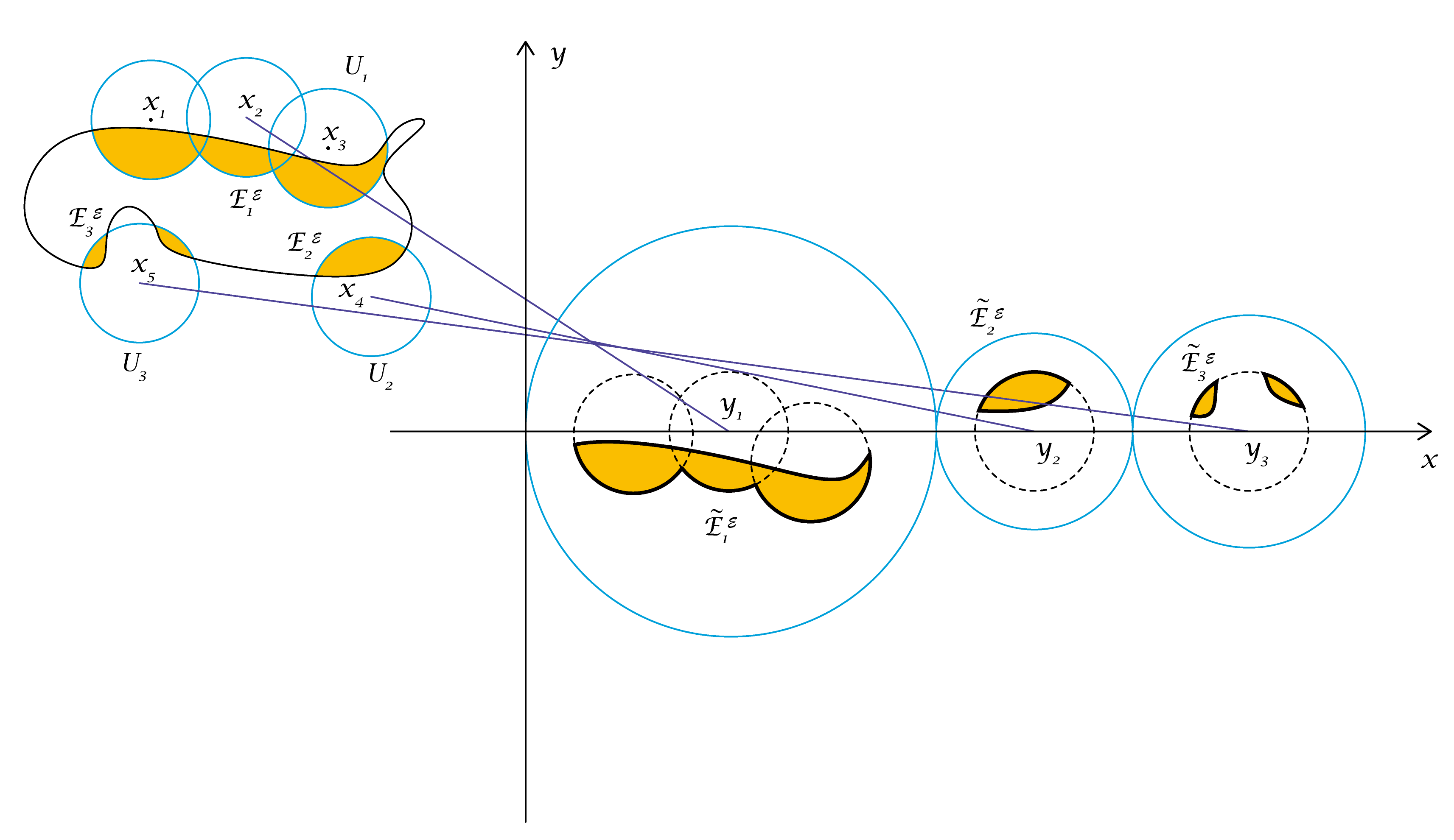
Figure 1: We use balls of fixed radius $r$ to cover the majority of $E$. For each connected part $E_{j}^{\varepsilon}$ combined with $F_{j}^{\varepsilon}$, we pack each pair $(E_{j}^{\varepsilon},F_{j}^{\varepsilon})$ into a ball and then align these balls together inside $B(O,R_{\varepsilon})$. For simplicity and clearness, we do not demonstrate corresponding parts from $F$.

Denote

$$E^{\varepsilon}\vcentcolon=E\cap U\quad\textrm{and}\quad E_{0}^{\varepsilon}\vcentcolon=E\setminus U.$$

Then, $E=E^{\varepsilon}\cup E_{0}^{\varepsilon}$,

$$\mathinner{\!\left\lvert E_{0}^{\varepsilon}\right\rvert}=\mathinner{\!\left\lvert E\setminus\bigcup_{x\in I}B(x,r)\right\rvert}<\varepsilon,\quad\textrm{and}\quad\mathinner{\!\left\lvert E^{\varepsilon}\right\rvert}=\mathinner{\!\left\lvert E\right\rvert}-\mathinner{\!\left\lvert E_{0}^{\varepsilon}\right\rvert}>\mathinner{\!\left\lvert E\right\rvert}-\varepsilon.$$

Since $\#I<\infty$, there are at most $\#I$ many connected components of $U$. Let $I=\bigsqcup_{j=1}^{k}I_{j}$, where $\left\{I_{1},I_{2},\cdots,I_{k}\right\}$ is a partition of $I$ and $k\leqslant\#I$, such that for each $j=1,2,\cdots,k$,

$$U_{j}\mathrel{\mathop{\ordinarycolon}}=\bigcup_{x\in I_{j}}B(x,r)$$

is a connected component of $U$. For each $j=1,2,\cdots,k$, denote

$$E_{j}^{\varepsilon}\vcentcolon=E\cap U_{j}.$$

Then $E^{\varepsilon}=\bigcup_{j=1}^{k}E^{\varepsilon}_{j}$, and $E_{j}^{\varepsilon}\subseteq U_{j}\subseteq B(x_{j},2rn_{j})$ for some point $x_{j}\in I_{j}$, where $n_{j}=\#I_{j}$ denotes the number of points in $I_{j}$.

Note that

$$\sum_{j=0}^{k}P(E_{j}^{\varepsilon})=P(E\setminus U)+P(E\cap U)=P(E)+2\mathcal{H}^{d-1}(E\cap\partial U\})\leqslant P(E)+2\varepsilon.$$ (5.2)

Since $\mathinner{\!\left\lvert F\right\rvert}=\mathinner{\!\left\lvert E\right\rvert}$ and $\mathinner{\!\left\lvert F\cap E\right\rvert}=0$, there exists an optimal transport map $\Phi$ that transports $E$ to $F$. For $j=1,2,\cdots,k$, let $F_{j}^{\varepsilon}\mathrel{\mathop{\ordinarycolon}}=\Phi(E_{j}^{\varepsilon})$ be the image of $E_{j}^{\varepsilon}$ under $\Phi$. Then

$$\sum_{j=1}^{k}W_{p}^{p}(E_{j}^{\varepsilon},F_{j}^{\varepsilon})=\sum_{j=1}^{k}\int_{E_{j}^{\varepsilon}}\mathinner{\!\left\lvert x-\Phi(x)\right\rvert}^{p}\mathop{}\!\mathrm{d}{\mathscr{L}^{d}(x)}=\int_{E^{\varepsilon}}\mathinner{\!\left\lvert x-\Phi(x)\right\rvert}^{p}\mathop{}\!\mathrm{d}{\mathscr{L}^{d}(x)}\leqslant W_{p}^{p}(E,F).$$ (5.3)

Now, let $\hat{F}_{j}^{\varepsilon}$ be a $\mathcal{W}_{p}$-minimizer of the bounded set $E^{\varepsilon}_{j}$. Then, $\mathinner{\!\left\lvert\hat{F}_{j}^{\varepsilon}\right\rvert}=\mathinner{\!\left\lvert E_{j}^{\varepsilon}\right\rvert}$, $\mathinner{\!\left\lvert\hat{F}_{j}^{\varepsilon}\cap E_{j}^{\varepsilon}\right\rvert}=0$ and

$$W_{p}(E_{j}^{\varepsilon},\hat{F}_{j}^{\varepsilon})\leqslant W_{p}(E_{j}^{\varepsilon},F_{j}^{\varepsilon}).$$

Since $E^{\varepsilon}_{j}\subseteq B(x_{j},2rn_{j})\subseteq B(x_{j},6n_{j})$, by (4.5) in Lemma 4.3, it follows that

$$\hat{F}_{j}^{\varepsilon}\subseteq B\left(x_{j},6n_{j}+C_{0}(d)\mathinner{\!\left\lvert E^{\varepsilon}_{j}\right\rvert}^{1/d}\right).$$

Note that

$$\sum_{j=1}^{k}\textrm{diam}\left(B\left(x_{j},6n_{j}+C_{0}(d)\mathinner{\!\left\lvert E^{\varepsilon}_{j}\right\rvert}^{1/d}\right)\right)$$

$$= \sum_{j=1}^{k}\left(12n_{j}+2C_{0}(d)\mathinner{\!\left\lvert E^{\varepsilon}_{j}\right\rvert}^{1/d}\right)=12\cdot\#I+2C_{0}(d)\sum_{j=1}^{k}\mathinner{\!\left\lvert E^{\varepsilon}_{j}\right\rvert}^{1/d}$$

$$\leqslant 12\cdot\#I+2C_{0}(d)k^{1-\frac{1}{d}}\left(\sum_{j=1}^{k}\mathinner{\!\left\lvert E^{\varepsilon}_{j}\right\rvert}\right)^{1/d}\leqslant 12\cdot\#I+2C_{0}(d)(\#I)^{1-\frac{1}{d}}\mathinner{\!\left\lvert E\right\rvert}^{1/d}$$

$$\leqslant 12\mathinner{\!\left\lvert E\right\rvert}\left(\frac{P(E)}{c(d)\varepsilon}\right)^{d}+2C_{0}(d)\left(\mathinner{\!\left\lvert E\right\rvert}\left(\frac{P(E)}{c(d)\varepsilon}\right)^{d}\right)^{1-\frac{1}{d}}\mathinner{\!\left\lvert E\right\rvert}^{1/d}$$

$$= 12\mathinner{\!\left\lvert E\right\rvert}\left(\frac{P(E)}{c(d)\varepsilon}\right)^{d}+2C_{0}(d)\left(\frac{P(E)}{c(d)\varepsilon}\right)^{d-1}\mathinner{\!\left\lvert E\right\rvert}=2R_{\varepsilon}-2\rho_{\varepsilon},$$

where

$$\rho_{\varepsilon}=\left(\frac{2\varepsilon}{\omega_{d}}\right)^{1/d}.$$

Thus, inside the ball $B(O,R_{\varepsilon})$, one may pick $k+1$ pairwise disjoint closed balls

$$\{\overline{B(y_{j},6n_{j}+C_{0}(d)\lvert E^{\varepsilon}_{j}\rvert^{1/d})}\}_{j=1}^{k}\cup\overline{B(y_{0},\rho_{\varepsilon})}.$$

For each $j=1,\cdots,k$, define

$$\widetilde{E}_{j}^{\varepsilon}=E_{j}^{\varepsilon}+(y_{j}-x_{j})\quad\textrm{and}\quad\widetilde{F}_{j}^{\varepsilon}=\hat{F}_{j}^{\varepsilon}+(y_{j}-x_{j}).$$

i.e., we translate the pair $(E_{j}^{\varepsilon},\hat{F}_{j}^{\varepsilon})$ in the ball $B(x_{j},6n_{j}+C_{0}(d)\mathinner{\!\left\lvert E^{\varepsilon}_{j}\right\rvert}^{1/d})$ to the corresponding pair $(\widetilde{E}_{j}^{\varepsilon},\widetilde{F}_{j}^{\varepsilon})$ inside the ball $B(y_{j},6n_{j}+C_{0}(d)|E^{\varepsilon}_{j}|^{1/d})$, as shown see Figure 1.

Since both the perimeter and the Wasserstein distance are translation invariant, we have

$$P(\widetilde{E}_{j}^{\varepsilon})=P(E_{j}^{\varepsilon})\quad\textrm{and}\quad W_{p}(\widetilde{E}_{j}^{\varepsilon},\widetilde{F}_{j}^{\varepsilon})=W_{p}(E_{j}^{\varepsilon},\hat{F}_{j}^{\varepsilon}).$$

Also denote

$$\widetilde{F}_{0}^{\varepsilon}\vcentcolon=B(y_{0},t_{\varepsilon})\setminus B(y_{0},s_{\varepsilon})\quad\textrm{and}\quad\widetilde{E}_{0}^{\varepsilon}\vcentcolon=B(y_{0},s_{\varepsilon}),$$

with

$$t_{\varepsilon}=\left(\frac{2\mathinner{\!\left\lvert E_{0}^{\varepsilon}\right\rvert}}{\omega_{d}}\right)^{1/d}\quad\textrm{and}\quad s_{\varepsilon}=\left(\frac{\mathinner{\!\left\lvert E_{0}^{\varepsilon}\right\rvert}}{\omega_{d}}\right)^{1/d}.$$

Note that

$$\mathinner{\!\left\lvert\widetilde{E}_{0}^{\varepsilon}\right\rvert}=\mathinner{\!\left\lvert E_{0}^{\varepsilon}\right\rvert}=\mathinner{\!\left\lvert\widetilde{F}_{0}^{\varepsilon}\right\rvert}.$$

Since $\mathinner{\!\left\lvert E_{0}^{\varepsilon}\right\rvert}\leqslant\varepsilon$, it follows that $0<s_{\varepsilon}<t_{\varepsilon}\leqslant\rho_{\varepsilon}$. Therefore, both sets $\widetilde{E}_{0}^{\varepsilon}$ and $\widetilde{F}_{0}^{\varepsilon}$ are contained in $B(y_{0},\rho_{\varepsilon})$. Now, define

$$\widetilde{E}\vcentcolon=\bigcup_{j=0}^{k}\widetilde{E}_{j}^{\varepsilon}\quad\textrm{and}\quad\widetilde{F}\vcentcolon=\bigcup_{j=0}^{k}\widetilde{F}_{j}^{\varepsilon}.$$

Then

$$\mathinner{\!\left\lvert\widetilde{E}\cap\widetilde{F}\right\rvert} =\mathinner{\!\left\lvert\bigcup_{j=0}^{k}\widetilde{E}_{j}^{\varepsilon}\cap\bigcup_{j=0}^{k}\widetilde{F}_{j}^{\varepsilon}\right\rvert}=\sum_{j=0}^{k}\mathinner{\!\left\lvert\widetilde{E}_{j}^{\varepsilon}\cap\widetilde{F}_{j}^{\varepsilon}\right\rvert}=0,$$

$$\mathinner{\!\left\lvert\widetilde{E}\right\rvert} =\sum_{j=0}^{k}\mathinner{\!\left\lvert\widetilde{E}_{j}^{\varepsilon}\right\rvert}=\sum_{j=0}^{k}\mathinner{\!\left\lvert E_{j}^{\varepsilon}\right\rvert}=\mathinner{\!\left\lvert E\right\rvert},$$

and similarly $\mathinner{\!\left\lvert\widetilde{F}\right\rvert}=\mathinner{\!\left\lvert F\right\rvert}$. As a result, $(\widetilde{E},\widetilde{F})\in\mathcal{F}$.

Moreover, by applying the isoperimetric inequality on $\widetilde{E}_{0}^{\varepsilon}$, (5.2) implies that

$$P(\widetilde{E})=\sum_{j=0}^{k}P(\widetilde{E}_{j}^{\varepsilon})\leqslant\sum_{j=0}^{k}P({E}_{j}^{\varepsilon})\leqslant P(E)+2\varepsilon.$$

Furthermore,

$$W_{p}^{p}(\widetilde{E},\widetilde{F}) \leqslant\sum_{j=0}^{k}W_{p}^{p}(\widetilde{E}_{j}^{\varepsilon},\widetilde{F}_{j}^{\varepsilon})$$

$$=W_{p}^{p}(\widetilde{E}_{0}^{\varepsilon},\widetilde{F}_{0}^{\varepsilon})+\sum_{j=1}^{k}W_{p}^{p}(E_{j}^{\varepsilon},F_{j}^{\varepsilon})$$

$$\leqslant(t_{\varepsilon})^{p}\mathinner{\!\left\lvert E_{0}^{\varepsilon}\right\rvert}+\sum_{j=1}^{k}W_{p}^{p}(E_{j}^{\varepsilon},F_{j}^{\varepsilon})$$

$$\leqslant\left(\frac{2\varepsilon}{\omega_{d}}\right)^{p/d}\varepsilon+W_{p}^{p}(E,F),$$

by (5.3). Thus, since $p\geqslant 1$, it follows that

$$W_{p}(\widetilde{E},\widetilde{F})\leqslant\left(\left(\frac{2\varepsilon}{\omega_{d}}\right)^{p/d}\varepsilon+W_{p}^{p}(E,F)\right)^{1/p}\leqslant\left(\frac{2\varepsilon}{\omega_{d}}\right)^{1/d}\varepsilon^{1/p}+W_{p}(E,F).$$

∎

Now we use Theorem 5.4 to prove Theorem 5.1.

Proof of Theorem 5.1.

Let $\left\{(E_{n},F_{n})\right\}$ be any minimizing sequence of the functional $P(E)+W_{p}(E,F)$ in $\mathcal{F}_{m}$. For each $n$, pick $\varepsilon_{n}$ small enough so that

$$0<\varepsilon_{n}\leqslant\min\left\{\frac{1}{n},m,~{}\frac{P(E_{n})}{2dc(d)}\right\}.$$

By Theorem 5.4, there exist bounded sets $(\widetilde{E_{n}},\widetilde{F_{n}})\in\mathcal{F}_{m}$ contained in the ball $B(O,R_{\varepsilon_{n}})$, such that

$$P(\widetilde{E_{n}})\leqslant P(E_{n})+\frac{2}{n},\quad\textrm{and}\quad W_{p}(\widetilde{E_{n}},\widetilde{F_{n}})\leqslant W_{p}(E_{n},F_{n})+\left(\frac{2}{\omega_{d}}\right)^{1/d}\left(\frac{1}{n}\right)^{\frac{1}{p}+\frac{1}{d}}.$$

Thus,

$$P(\widetilde{E_{n}})+W_{p}(\widetilde{E_{n}},\widetilde{F_{n}})\leqslant P(E_{n})+W_{p}(E_{n},F_{n})+\frac{2}{n}+\left(\frac{2}{\omega_{d}}\right)^{1/d}\left(\frac{1}{n}\right)^{\frac{1}{p}+\frac{1}{d}}.$$

This shows the sequence of the bounded sets $\left\{(\widetilde{E_{n}},\widetilde{F_{n}})\right\}$ is also a minimizing sequence of the functional $P(E)+W_{p}(E,F)$ in $\mathcal{F}_{m}$. ∎

Corollary 5.5.

For any $m\geqslant 0$, the minimizing problem (3.8) is equivalent to the problem

$$\text{ Minimize }\qquad P(E)+W_{p}(E,F)\qquad\text{ among all bounded sets }(E,F)\in\mathcal{F}_{m}.$$ (5.4)

To solve problem (5.4), it is sufficient to solve the problem

$$\text{ Minimize }\qquad T(E)\mathrel{\mathop{\ordinarycolon}}=P(E)+\mathcal{W}_{p}(E)$$ (5.5)

among all bounded set $E\subseteq\mathbb{R}^{d}$ of finite perimeter with $\mathinner{\!\left\lvert E\right\rvert}=m$. Any solution $E^{*}$ of problem (5.5) together with its $\mathcal{W}_{p}$-minimizer $F^{*}$ provides a solution $(E^{*},F^{*})$ to problem (5.4), and vice versa.

6 Existence of minimizers for small volume

In this section, we will show that problem (5.5) has a solution when $m$ is small and $\frac{1}{p}+\frac{2}{d}>1$. Our work is inspired by [KM14] as mentioned in the introduction.

Theorem 6.1.

Suppose $d\geqslant 1,p\geqslant 1$ with $\frac{1}{p}+\frac{2}{d}>1$, there exists an $m_{0}>0$ such that for any $m\leqslant m_{0}$, the minimization problem (5.5) has a solution.

Recall Theorem 6.1 is equivalent to Theorem 1.1 and Theorem 3.5.

To do so, we start with a few technique propositions.

Proposition 6.2 (Nonoptimality).

Suppose $d\geqslant 1,p\geqslant 1$ with $\frac{1}{p}+\frac{2}{d}>1$, let $G\subseteq\mathbb{R}^{d}$ be a bounded set of finite perimeter with $\mathinner{\!\left\lvert G\right\rvert}=m<\min\{1,\omega_{d}\}$. Suppose there is a partition of $G$ into two disjoint sets of finite perimeter $G_{1}$ and $G_{2}$ with positive volumes such that

$$P(G_{1})+P(G_{2})-P(G)\leqslant\frac{1}{2}T(G_{2}).$$ (6.1)

Then there is an $\varepsilon=\varepsilon(m,d)>0$ such that if

$$\mathinner{\!\left\lvert G_{2}\right\rvert}\leqslant\varepsilon\mathinner{\!\left\lvert G_{1}\right\rvert},$$

there exists a bounded set $E\subseteq\mathbb{R}^{d}$ such that $\mathinner{\!\left\lvert E\right\rvert}=\mathinner{\!\left\lvert G\right\rvert}$ and $T(E)<T(G)$.

Figure 2: If a set $G$ can be split into a dominated part $G_{1}$ and a remainder part $G_{2}$, with a small slicing surface area bounded by $\frac{1}{4}T(G_{2})$, then $G$ may not be a $T$-minimizer.

Proof.

Let $r\mathrel{\mathop{\ordinarycolon}}=\left(\frac{m}{\omega_{d}}\right)^{1/d}<1$. Then $\mathinner{\!\left\lvert B_{r}\right\rvert}=\omega_{d}r^{d}=m=\mathinner{\!\left\lvert G\right\rvert}$. When $T(B_{r})<T(G)$, the result holds for $E=B_{r}$. Thus, without loss of generality, we may assume that $T(B_{r})\geqslant T(G)$.

By direct computation and (4.4) in Lemma 4.3,

$$P(B_{r})=d\omega_{d}r^{d-1}=d\omega_{d}^{1/d}m^{1-1/d}\quad\textrm{and}\quad\mathcal{W}_{p}(B_{r})\leqslant C_{0}(d)m^{\frac{1}{p}+\frac{1}{d}},$$

thus,

$$T(G)\leqslant T(B_{r})\leqslant C(d)\max{(m^{1/p+1/d},m^{1-1/d})}\leqslant C(d)m^{1-1/d},$$ (6.2)

because $\frac{1}{p}+\frac{1}{d}>1-\frac{1}{d}$ and $m<1$. Since $G$ is the disjoint union of $G_{1}$ and $G_{2}$, it follows that

$$\mathcal{W}_{p}(G_{1})+\mathcal{W}_{p}(G_{2})-\mathcal{W}_{p}(G)\leqslant 0.$$ (6.3)

Together with (6.1), it follows that

$$T(G_{1})+T(G_{2})-T(G)\leqslant\frac{1}{2}T(G_{2}),$$

i.e.

$$T(G_{1})+\frac{1}{2}T(G_{2})\leqslant T(G).$$ (6.4)

Let

$$\gamma=\frac{\mathinner{\!\left\lvert G_{2}\right\rvert}}{\mathinner{\!\left\lvert G_{1}\right\rvert}},\ \ell=(1+\gamma)^{1/d},\quad\textrm{and}\quad E=\ell G_{1}.$$

Note that when $\frac{1}{p}+\frac{2}{d}>1$, it follows that $d-1<1+\frac{d}{p}$. Note that $\ell>1$, thus

$$T(E)=\ell^{d-1}P(G_{1})+\ell^{1+d/p}\mathcal{W}_{p}(G_{1})\leqslant\ell^{1+d/p}(P(G_{1})+\mathcal{W}_{p}(G_{1}))=\ell^{1+d/p}T(G_{1}).$$

As a result,

$$T(E)-T(G) \leqslant T(G_{1})-T(G)+(\ell^{1+d/p}-1)T(G_{1})$$

$$=T(G_{1})+T(G_{2})-T(G)-T(G_{2})+(\ell^{1+d/p}-1)T(G_{1})$$

$$=\left(P(G_{1})+P(G_{2})-P(G)\right)+\left(\mathcal{W}_{p}(G_{1})+\mathcal{W}_{p}(G_{2})-\mathcal{W}_{p}(G)\right)-T(G_{2})+(\ell^{1+d/p}-1)T(G_{1})$$

$$\stackrel{{\scriptstyle\eqref{eq: cond_nonopt}}}{{\leqslant}}\frac{1}{2}T(G_{2})+0-T(G_{2})+(\ell^{1+d/p}-1)T(G_{1}),$$

$$=-\frac{1}{2}T(G_{2})+(\ell^{1+d/p}-1)T(G_{1})$$

$$=-\frac{1}{2}T(G_{2})+((1+\gamma)^{1/d+1/p}-1)T(G_{1})$$

$$\leqslant-\frac{1}{2}T(G_{2})+2(1/d+1/p)\gamma T(G_{1})$$

when $\gamma>0$ is small enough. By isoperimetric inequality, we have

$$T(G_{2})\geqslant P(G_{2})\geqslant C(d)\mathinner{\!\left\lvert G_{2}\right\rvert}^{1-1/d}.$$

On the other hand, by (6.4) and (6.2), when $\gamma<1/2$,

$$\gamma T(G_{1})\leqslant\gamma T(G)\leqslant C(d)\gamma m^{1-1/d}=C(d)\gamma^{1/d}(\gamma m)^{1-1/d}\leqslant C(d)\gamma^{1/d}(2\mathinner{\!\left\lvert G_{2}\right\rvert})^{1-1/d}.$$

Hence, combine those inequalities, we have

$$T(E)-T(G) \leqslant-C(d)\mathinner{\!\left\lvert G_{2}\right\rvert}^{1-1/d}+C(d)\gamma^{1/d}\mathinner{\!\left\lvert G_{2}\right\rvert}^{1-1/d}$$

$$\leqslant-C(d)\mathinner{\!\left\lvert G_{2}\right\rvert}^{1-1/d}+C(d)\varepsilon^{1/d}\mathinner{\!\left\lvert G_{2}\right\rvert}^{1-1/d}$$

$$<0,$$

for $\varepsilon$ sufficiently small. ∎

Using the above proposition, we have the following uniform boundedness result:

Theorem 6.3.

Suppose $p\geqslant$, $d\geqslant 1$ with $\frac{1}{p}+\frac{2}{d}>1$, there exists an $m_{0}>0$ such that for every bounded set $G\subseteq\mathbb{R}^{d}$ of finite perimeter with $\mathinner{\!\left\lvert G\right\rvert}\leqslant m_{0}$, there exists a bounded set $E\subseteq\mathbb{R}^{d}$ of finite perimeter with

$$\mathinner{\!\left\lvert E\right\rvert}=\mathinner{\!\left\lvert G\right\rvert},\qquad T(E)\leqslant T(G)\quad\textrm{and}\quad E\subseteq B_{2}.$$ (6.5)

Proof.

We may assume $m\mathrel{\mathop{\ordinarycolon}}=\mathinner{\!\left\lvert G\right\rvert}\leqslant\min\{1,\omega_{d}\}$, and set $r\mathrel{\mathop{\ordinarycolon}}=\left(\frac{m}{\omega_{d}}\right)^{1/d}$. Note that $r\leqslant 1$ and $\mathinner{\!\left\lvert B_{r}\right\rvert}=\omega_{d}r^{d}=\mathinner{\!\left\lvert G\right\rvert}$. Thus, when $T(G)\geqslant T(B_{r})$, the set $E=B_{r}$ satisfies (6.5). As a result, without loss of generality, we may assume that

$$T(G)<T(B_{r}).$$

That is,

$$P(G)+\mathcal{W}_{p}(G)<P(B_{r})+\mathcal{W}_{p}(B_{r}).$$

Thus, we have the following upper bound for the isoperimetric deficit of $G$:

$$D(G) =\frac{P(G)-P(B_{r})}{P(B_{r})}<\frac{\mathcal{W}_{p}(B_{r})-\mathcal{W}_{p}(G)}{P(B_{r})}$$

$$\leqslant\frac{\mathcal{W}_{p}(B_{r})}{P(B_{r})}\leqslant\frac{C_{0}(d)\mathinner{\!\left\lvert B_{r}\right\rvert}^{\frac{1}{p}+\frac{1}{d}}}{P(B_{r})}$$

$$=\frac{C_{0}(d)(\omega_{d}r^{d})^{\frac{1}{p}+\frac{1}{d}}}{d\omega_{d}r^{d-1}}=\frac{C_{0}(d)}{d(\omega_{d})^{1-\frac{1}{p}-\frac{1}{d}}}r^{\alpha},$$

where $\alpha\mathrel{\mathop{\ordinarycolon}}=2+d(\frac{1}{p}-1)>0$. By (3.3), and up to a suitable translation, we have

$$\frac{\mathinner{\!\left\lvert G\setminus B_{r}\right\rvert}}{\mathinner{\!\left\lvert G\right\rvert}} \leqslant\frac{\mathinner{\!\left\lvert G\Delta B_{r}\right\rvert}}{\mathinner{\!\left\lvert G\right\rvert}}=\Delta(G,B_{r})\leqslant C(d)\sqrt{D(G)}$$

$$\leqslant C(d)\sqrt{\frac{C_{1}(d,p)}{d(\omega_{d})^{1-\frac{1}{p}-\frac{1}{d}}}r^{\alpha}}=C(d,p)r^{\alpha/2},$$ (6.6)

where

$$C(d,p)=C(d)\sqrt{\frac{C_{1}(d,p)}{d(\omega_{d})^{1-\frac{1}{p}-\frac{1}{d}}}}.$$

Let $m_{0}>0$ be small enough such that

$$C(d,p)(\frac{m_{0}}{\omega_{d}})^{\alpha/2}<1.$$

Then,

$$C(d,p)r^{\alpha/2}=C(d,p)(\frac{m}{\omega_{d}})^{\alpha/2}<1.$$

Since the function $\frac{x}{1-x}$ is increasing on $[0,1)$, we have when $r>0$ is small enough,

$$\frac{\mathinner{\!\left\lvert G\setminus B_{r}\right\rvert}/\mathinner{\!\left\lvert G\right\rvert}}{1-\mathinner{\!\left\lvert G\setminus B_{r}\right\rvert}/\mathinner{\!\left\lvert G\right\rvert}}\leqslant\frac{C(d,p)r^{\alpha/2}}{1-C(d,p)r^{\alpha/2}}\leqslant\varepsilon,$$

where $\varepsilon$ is given in Proposition 6.2. That is,

$$\mathinner{\!\left\lvert G\setminus B_{r}\right\rvert}\leqslant\varepsilon\mathinner{\!\left\lvert G\cap B_{r}\right\rvert},$$

for $\mathinner{\!\left\lvert G\right\rvert}=\mathinner{\!\left\lvert G\setminus B_{r}\right\rvert}+\mathinner{\!\left\lvert G\cap B_{r}\right\rvert}$. Note that for all $t\geqslant r$, it also follows that

$$\mathinner{\!\left\lvert G\setminus B_{t}\right\rvert}\leqslant\varepsilon\mathinner{\!\left\lvert G\cap B_{t}\right\rvert}.$$

Case 1: When $P(G\cap B_{t})+P(G\setminus B_{t})-P(G)\leqslant\frac{1}{2}T(G\setminus B_{t})$ for some $t\in[r,1]$, by Proposition 6.2 there exists a bounded set $E$ with $T(E)\leqslant T(G)$. By the proof of Proposition 6.2, either $E=B_{r}\subseteq B_{2}$ or $E=\ell(G\cap B_{t})\subseteq\ell B_{t}\subseteq B_{2}$, where $\ell\leqslant(1+\varepsilon)^{1/d}\leqslant 2$.

Case 2: When $P(G\cap B_{t})+P(G\setminus B_{t})-P(G)\geqslant\frac{1}{2}T(G\setminus B_{t})$ for all $t\in[r,1]$, we have the following observations. By the coarea formula (see Proposition 1 in Section 3.4.4 in [EG92]), for almost every $t\in[r,1]$,

$$\frac{\mathrm{d}}{\mathop{}\!\mathrm{d}{t}}\mathinner{\!\left\lvert G\cap B_{t}\right\rvert} =\frac{\mathrm{d}}{\mathop{}\!\mathrm{d}{t}}\left(\int_{B_{t}}\mathbbm{1}_{G}\mathop{}\!\mathrm{d}{x}\right)$$

$$=\mathcal{H}^{d-1}(G\cap\partial B_{t})$$

$$=\frac{1}{2}(P(G\cap B_{t})+P(G\setminus B_{t})-P(G))$$

$$\geqslant\frac{1}{2}\cdot\frac{1}{2}T(G\setminus B_{t})$$

$$\geqslant\frac{1}{4}P(G\setminus B_{t})$$

$$\geqslant\frac{C(d)}{4}\mathinner{\!\left\lvert G\setminus B_{t}\right\rvert}^{1-1/d},$$

by the isoperimetric inequality. Thus, for almost every $t\in[r,1]$,

$$\frac{\mathrm{d}}{\mathop{}\!\mathrm{d}{t}}\mathinner{\!\left\lvert G\setminus B_{t}\right\rvert}=-\frac{\mathop{}\!\mathrm{d}{}}{\mathop{}\!\mathrm{d}{t}}\mathinner{\!\left\lvert G\cap B_{t}\right\rvert}\leqslant-\frac{C(d)}{4}\mathinner{\!\left\lvert G\setminus B_{t}\right\rvert}^{1-1/d}.$$

By Gronwall’s inequality, for all $t\in[r,1]$,

$$\mathinner{\!\left\lvert G\setminus B_{t}\right\rvert}^{1/d} \leqslant\max\{0,\mathinner{\!\left\lvert G\setminus B_{r}\right\rvert}^{1/d}-\frac{C(d)}{4d}(t-r)\}$$

$$\stackrel{{\scriptstyle\eqref{eq: volume_rate}}}{{\leqslant}}\max\{0,\left(C(d,p)\mathinner{\!\left\lvert G\right\rvert}r^{\alpha/2}\right)^{1/d}-\frac{C(d)}{4d}(t-r)\}$$

$$=\max\{0,\left(C(d,p)w_{d}\right)^{1/d}r^{1+\alpha/{2d}}-\frac{C(d)}{4d}(t-r)\}.$$

In particular,

$$\mathinner{\!\left\lvert G\setminus B_{1}\right\rvert}^{1/d}\leqslant\max\{0,\left(C(d,p)w_{d}\right)^{1/d}r^{1+\alpha/{2d}}-\frac{C(d)}{4d}(1-r)\}=0$$

whenever $r$ is sufficiently small. Hence, for $r$ sufficiently small, it holds that $\mathinner{\!\left\lvert G\setminus B_{1}\right\rvert}=0$, and the set $E=G$ satisfies (6.5).

∎

Thanks to Theorem 6.3, we are able to apply the direct method to prove Theorem 6.1.

Proof of Theorem 6.1.

Let $(G_{k})$ be a minimizing sequence to problem (5.5) with each $G_{k}$ being a bounded subset of $\mathbb{R}^{d}$ and $\mathinner{\!\left\lvert G_{k}\right\rvert}=m$. By Theorem 6.3, there exists an alternating minimizing sequence $(E_{k})$ to problem (5.5) with $\mathinner{\!\left\lvert E_{k}\right\rvert}=m$, which is uniformly bounded by $B_{2}$. By the compactness of bounded sets of finite perimeter (Proposition 3.2), there exists a set $E$ of finite perimeter in $\mathbb{R}^{d}$, such that up to extracting a subsequence if necessary:

$$E_{k}\to E\quad\textrm{and}\quad E\subseteq B_{2}.$$

By the lower semi-continuity of $\mathcal{W}_{p}$ (Lemma 4.4) and the lower semi-continuity of perimeter (Proposition 3.1), $T$ is lower semi-continuous. Thus,

$$T(E)\leqslant\liminf_{k\to\infty}T(E_{k}),$$

which yields that $E$ is a minimizer to problem (5.5). ∎

QINGLAN XIA, Department of Mathematics, University of California at Davis

E-mail address: qlxia@math.ucdavis.edu

BOHAN ZHOU, Department of Mathematics, University of California at Davis

E-mail address: bhzhouzhou@math.ucdavis.edu

References

- [Alm76] F. J. Almgren, Jr. Existence and regularity almost everywhere of solutions to elliptic variational problems with constraints. Mem. Amer. Math. Soc., 4(165):viii+199, 1976.
- [Amb03] L. Ambrosio. Lecture notes on optimal transport problems. In Mathematical aspects of evolving interfaces (Funchal, 2000), volume 1812 of Lecture Notes in Math., pages 1–52. Springer, Berlin, 2003.
- [BCL17] G. Buttazzo, G. Carlier, and M. Laborde. On the Wasserstein distance between mutually singular measures. Advances in Calculus of Variations, 2017.
- [Bre91] Y. Brenier. Polar factorization and monotone rearrangement of vector-valued functions. Comm. Pure Appl. Math., 44(4):375–417, 1991.
- [DMS19] S. Di Marino and F. Santambrogio. JKO estimates in linear and non-linear Fokker-Planck equations, and Keller-Segel: Lp and Sobolev bounds. arXiv preprint arXiv:1911.10999, 2019.
- [DPMSV16] G. De Philippis, A. Mészáros, F. Santambrogio, and B. Velichkov. BV estimates in optimal transportation and applications. Arch. Ration. Mech. Anal., 219(2):829–860, 2016.
- [EG92] L. Evans and R. Gariepy. Measure theory and fine properties of functions. Studies in Advanced Mathematics. CRC Press, Boca Raton, FL, 1992.
- [FFM+15] A. Figalli, N. Fusco, F. Maggi, V. Millot, and M. Morini. Isoperimetry and stability properties of balls with respect to nonlocal energies. Comm. Math. Phys., 336(1):441–507, 2015.
- [FMP08] N. Fusco, F. Maggi, and A. Pratelli. The sharp quantitative isoperimetric inequality. Ann. of Math. (2), 168(3):941–980, 2008.
- [FMP10] A. Figalli, F. Maggi, and A. Pratelli. A mass transportation approach to quantitative isoperimetric inequalities. Invent. Math., 182(1):167–211, 2010.
- [GM96] W. Gangbo and R. J. McCann. The geometry of optimal transportation. Acta Math., 177(2):113–161, 1996.
- [JKO98] R. Jordan, D. Kinderlehrer, and F. Otto. The variational formulation of the Fokker-Planck equation. SIAM J. Math. Anal., 29(1):1–17, 1998.
- [KM13] H. Knüpfer and C. B. Muratov. On an isoperimetric problem with a competing nonlocal term I: The planar case. Comm. Pure Appl. Math., 66(7):1129–1162, 2013.
- [KM14] H. Knüpfer and C. B. Muratov. On an isoperimetric problem with a competing nonlocal term II: The general case. Comm. Pure Appl. Math., 67(12):1974–1994, 2014.
- [LPR14] L. Lussardi, M.A. Peletier, and M. Röger. Variational analysis of a mesoscale model for bilayer membranes. J. Fixed Point Theory Appl., 15(1):217–240, 2014.
- [Mag12] F. Maggi. Sets of finite perimeter and geometric variational problems, volume 135 of Cambridge Studies in Advanced Mathematics. Cambridge University Press, Cambridge, 2012. An introduction to geometric measure theory.
- [Mil06] E. Milakis. On the regularity of optimal sets in mass transfer problems. Comm. Partial Differential Equations, 31(4-6):817–826, 2006.
- [Mor96] Frank Morgan. What is a surface? The American mathematical monthly, 103(5):369–376, 1996.
- [PR09] M. Peletier and M. Röger. Partial localization, lipid bilayers, and the elastica functional. Arch. Ration. Mech. Anal., 193(3):475–537, 2009.
- [San15] F. Santambrogio. Optimal transport for applied mathematicians, volume 87 of Progress in Nonlinear Differential Equations and their Applications. Birkhäuser/Springer, Cham, 2015. Calculus of variations, PDEs, and modeling.
- [San17] F. Santambrogio. {Euclidean, metric, and Wasserstein} gradient flows: an overview. Bull. Math. Sci., 7(1):87–154, 2017.
- [San18] F. Santambrogio. Crowd motion and evolution PDEs under density constraints. In SMAI 2017— Biennale Française des Mathématiques Appliquées et Industrielles, volume 64 of ESAIM Proc. Surveys, pages 137–157. EDP Sci., Les Ulis, 2018.
- [Vil03] C. Villani. Topics in optimal transportation, volume 58 of Graduate Studies in Mathematics. American Mathematical Society, Providence, RI, 2003.
- [Vil09] C. Villani. Optimal transport, volume 338 of Grundlehren der Mathematischen Wissenschaften [Fundamental Principles of Mathematical Sciences]. Springer-Verlag, Berlin, 2009. Old and new.
- [Xia05] Q. Xia. Regularity of minimizers of quasi perimeters with a volume constraint. Interfaces and free boundaries, 7(3):339–352, 2005.