Seeing Around Corners with Edge-Resolved Transient Imaging

Abstract

Non-line-of-sight (NLOS) imaging is a rapidly growing field seeking to form images of objects outside the field of view, with potential applications in search and rescue, reconnaissance, and even medical imaging. The critical challenge of NLOS imaging is that diffuse reflections scatter light in all directions, resulting in weak signals and a loss of directional information. To address this problem, we propose a method for seeing around corners that derives angular resolution from vertical edges and longitudinal resolution from the temporal response to a pulsed light source. We introduce an acquisition strategy, scene response model, and reconstruction algorithm that enable the formation of 2.5-dimensional representations – a plan view plus heights – and a 180$\degree$ field of view (FOV) for large-scale scenes. Our experiments demonstrate accurate reconstructions of hidden rooms up to 3 meters in each dimension.

Department of Electrical and Computer Engineering, Boston University, 1 Silber Way, Boston, Massachusetts 02215, USA

Charles Stark Draper Laboratory, Inc., 555 Technology Square, Cambridge, Massachusetts 02139, USA

School of Engineering and Physical Sciences, Heriot-Watt University, Edinburgh, EH14 4AS, UK

Department of Computer Science and Engineering, University of South Florida, 4202 E. Fowler Avenue, Tampa, Florida 33620, USA

INP/ENSEEHIT-IRIT-TeSA, University of Toulouse, 31071 Toulouse Cedex 7, France

Research Laboratory of Electronics, Massachusetts Institute of Technology, 77 Massachusetts Avenue, Cambridge, Massachusetts 02139, USA.

These authors contributed equally.

Significant strides have been made over the past decade to enable imaging beyond the line of sight[1, 2, 3, 4, 5, 6, 7, 8, 9, 10, 11, 12, 13, 14, 15, 16, 17, 18, 19, 20, 21, 22]. However, all of the proposed methods must contend with a pair of challenges resulting from diffuse reflections: the scattering of light destroys directional information and diminishes the intensity as the inverse-square of the distance. For line-of-sight (LOS) imaging (e.g., conventional photography or lidar), the effect of the diffuse reflection of the illumination toward a detector is minor because the directionality of light can be preserved through focused illumination or detection, and the radial falloff is often only a problem at large stand-off distances. The difficulty of NLOS imaging arises because of the cascaded diffuse reflections[9]. For passive NLOS imaging methods[1, 2, 3, 4, 5], ambient illumination bounces off a hidden scene and a relay surface (usually a visible wall or floor) before reaching a detector. Actively-illuminated approaches incur at least three diffuse reflections: from a visible relay surface to the hidden scene, off the scene, and back from the relay to the detector[8, 9, 10, 11, 12, 6, 7, 13, 14, 15, 16, 17, 18, 19, 20]. Some NLOS imaging approaches aim to avoid diffuse reflections entirely by using modalities (e.g., thermal[21], acoustic[22], or radar[23]) operating at long wavelengths, at which optically-rough surfaces appear smooth. While the directionality and signal strength are preserved through one or more specular reflections, such methods measure physical properties other than the optical reflectance, the resolution is lower due to the longer wavelengths, and the specular reflections can lead to confusion in distinguishing between direct and indirect reflections.

The first challenge for optical NLOS imaging is how to recover directional information from diffusely reflected light. One approach is to use active optical illumination and time-resolved sensing, for which the high-resolution transient information constrains the reconstruction of possible light directions to a more feasible inverse problem[9, 10, 11, 12, 13, 14, 15, 16, 17, 18, 19, 20]. Methods that do not capture temporal information[1, 2, 3, 4, 5, 6, 7, 24] – especially those using passive illumination – require a different approach to recovering directionality, such as by taking advantage of occlusions that block certain light paths and reduce directional uncertainty, similar to coded-aperture imaging or reference structure tomography[25]. Other methods use temporal differences between measurements to remove the contributions from static scene components, enabling improved resolution of an object in motion[1, 12, 26].

The second main challenge is handling extremely low levels of informative light for macroscopic scenes. Although active methods typically use single-photon detection and acquire transient information from many repeated illuminations, the hidden scene is still generally limited to around 1 meter from the relay surface. Examples that form images of objects at the greatest distances or with the lowest acquisition times increase the laser illumination power to levels that are not eye-safe (e.g., 1 W average optical power at 532 nm)[17, 18]. Passive, intensity-only methods generally have less radial fall-off but more uncertainty due to uninformative ambient light, so reconstructions are typically limited to 2D images of table-top scenes[3] or 1D traces showing objects’ angular positions with respect to a vertical edge[1, 4].

This work recovers large-scale 3D NLOS images with a large field-of-view (FOV) by combining concepts from both active and passive methods for separating contributions mixed by diffuse reflection into a novel acquisition configuration. We call our method edge-resolved transient imaging (ERTI) because we take advantage of occlusions from vertical edges, in addition to using single-photon-sensitive, time-resolved acquisition. Our method introduces a dual configuration to existing “corner cameras” by scanning a light source along an arc on the ground plane around a vertical edge, thereby controlling which portion of the hidden space is illuminated, and detecting light from a single spot. Combining pulsed illumination and time-resolved, single-photon sensing yields measurements of the transient response of the illuminated scene. Because of the novel acquisition geometry, differences between histograms of photon detection times from adjacent illumination spots localize the transient response to that of a hemispherical wedge. Light propagation modelling leads to closed-form expressions for the temporal response functions of planar facets extending from the ground plane for a given distance, height, orientation, and albedo. Bayesian inference employing a tailored Markov chain Monte Carlo (MCMC) sampling approach reconstructs planar facets for each wedge and accounts for prior beliefs about the structure of likely scenes.

Results

0.1 Acquisition Methodology.

Vertical edges, such as those in door frames or at the boundaries of buildings, are ubiquitous and have proved useful for passive NLOS imaging[1, 4]. In so-called “corner cameras”, a conventional camera images the ground plane where it intersects with the vertical edge of a wall separating visible and hidden scenes. Whereas light from any visible part of the scene can reach the camera’s FOV, the vertical edge occludes light from the hidden scene from reaching certain pixels, depending on their position relative to the vertical edge. This work introduces two changes to how vertical edges enable NLOS imaging. First, rather than using global illumination and spatially-resolved detection, we propose a Helmholtz reciprocal dual of the edge camera, in which the illumination is scanned along an arc centered at the edge, and a bucket detector aimed beyond the edge collects light from both the visible and hidden scenes. Second, we use a pulsed laser and single-photon-sensitive, time-resolved detection instead of a conventional camera.

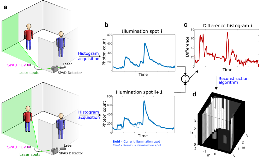
Figure 1: ERTI scenario and procedure. a, Positions along an arc centred on the occluding wall edge are illuminated sequentially by a pulsed laser. b, A histogram over time of photon detections is collected for each laser illumination position. The measured histograms contain photons reflected from both the hidden scene and the visible side. c, Taking differences between sequential histograms on average yields returns originating only from a small wedge within the hidden scene. d, A hidden area reconstruction using the collection of histogram differences.

The ERTI acquisition methodology is illustrated in Fig. 1. A 532-nm laser at 120 mW average optical power sequentially illuminates 45 spots evenly spaced in angle $\theta$ from $0$ to $\pi$ radians along a semicircle of radius 1.5 cm centred around the edge of the wall. The laser light illuminates an increasing fraction of the hidden scene as the illumination spot moves along the arc toward the hidden area. Each spot $i$ is repeatedly illuminated with picosecond-duration pulses at 20-MHz repetition rate for a preset dwell time. Light from each pulse bounces off the Lambertian ground plane and scatters in all directions, reflecting from surfaces in both visible and hidden portions of the scene. A single-photon avalanche diode (SPAD) detector is focused at a small spot roughly 20 cm beyond the vertical edge, enabling collection of light from the entire hidden scene for each illumination spot. After each pulse, a time-correlated single photon counting (TCSPC) module connected to the SPAD records photon detection times with 16-ps resolution, forming a histogram $\mathbf{m}_{i}$ of those photons reflected back to the SPAD. To prevent the direct reflection from overwhelming the much weaker light from the hidden scene, temporal gating is implemented to turn on 3 ns after the direct reflection from the ground reaches the SPAD.

The detected light intensity for spot $i$ includes contributions $\mathbf{h}_{i}$ from the hidden scene, $\mathbf{v}_{i}$ from the visible scene, and $\mathbf{b}$ from the background (a combination of ambient light and dark counts). The background is assumed to have constant intensity over the duration of the acquisition, and because the illumination arc radius is small, the visible scene contribution is approximately constant over all spots, i.e., $\mathbf{v}_{i}\approx\mathbf{v}_{j}$ for all $i,j$. However, illuminating sequentially along an arc will change the parts of the hidden scene that are illuminated. More precisely, a larger area of the hidden scene is illuminated as $i$ increases, so $\mathbf{h}_{i+1}=\mathbf{h}_{i}+\mathbf{u}_{i}$, where $\mathbf{u}_{i}$ is the component of the histogram contributed by the portion of the scene illuminated from spot $i+1$ but not from spot $i$, and $\mathbf{u}_{0}=\mathbf{0}$ because only the visible scene is illuminated from the first laser spot. The key idea behind ERTI is that this new contribution can be isolated – thereby regaining NLOS directionality – by considering the difference between successive histograms, that is,

$$\mathbf{y}_{i} =\mathbf{m}_{i+1}-\mathbf{m}_{i}\approx\left(\mathbf{v}_{i+1}+\mathbf{b}+\sum_{j=0}^{i}\mathbf{u}_{j}\right)-\left(\mathbf{v}_{i}+\mathbf{b}+\sum_{j=0}^{i-1}\mathbf{u}_{j}\right)\approx\mathbf{u}_{i}.$$ (1)

Due to the hemispherical reflection of light from a Lambertian ground plane and the occlusion effect of the vertical edge, the histogram differences $\{\mathbf{y}_{i}\}_{i=1,\dots,44}$ correspond to distinct wedges fanned out from the vertical edge. We note that each photon detection time histogram $\mathbf{m}_{i}$ has Poisson-distributed entries, so each histogram difference $\mathbf{y}_{i}$ has entries following the Poisson-difference or Skellam distribution[27]. Moreover, the entries of $\mathbf{y}_{i}$ are conditionally independent given the scene configuration. Note that although the mean visible scene and ambient light contributions are removed by this procedure, they do still contribute to the variance of the observation noise; see Supplementary Section 2, which discusses how working with $\mathbf{y}_{i}$ directly instead of $\mathbf{m}_{i}$ leads to a more efficient reconstruction procedure.

0.2 Light Transport Model.

Whereas active NLOS methods typically attempt full 3D reconstructions, and passive edge cameras form a 1D representation of the hidden scene, ERTI produces an intermediate “2.5D” representation, augmenting a 2D plan view (the positions and orientations of surfaces in the hidden space) with the height of each surface. This representation is chosen as a compromise between the acquisition method, which measures polar coordinate parameters (azimuth from the position with respect to the vertical edge and range from the time-resolved sensing), and typical scenes, which are more naturally represented as being composed of planar facets than spherical or cylindrical shells. Although there is no similarly direct mechanism to measure elevation angle, the duration of the temporal response from a scene patch contains information about its spatial extent and orientation. To regularize the reconstruction problem, we use the fact that most commonplace objects in the scene, such as humans, walls or furniture, present a base that starts from the ground plane. Using this assumption, the temporal response profile of a wedge then provides local height information about the hidden scene. Consequently, we suppose that hidden scenes can be coarsely described by uniform-albedo vertical planar facets extending up from the ground plane. Because considering histogram differences isolates the response from a single wedge, we can compute the response for each wedge of the hidden scene independently. For indoor scenes, we also model the presence of a ceiling as a single additional surface, assumed parallel to the ground. Despite being a major exception to our vertical facet model, inclusion of the ceiling component is necessary as it often reflects a significant amount of light.

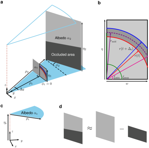
Figure 2: Planar facet scene representation. a, The contents of a wedge spanning angle $\Delta_{\theta}$ are represented by a set of planar facets parameterized by a distance $\rho$, height $\eta$, albedo $\alpha$, and orientation angle $\phi$. b, The basic transient light transport is computed for the region illuminated between times $t$ and $t+\Delta_{t}$ of one-half of a fronto-parallel facet. For facets with nonzero $\phi$, the full response linearly combines two half-facet responses with the distance and widths adjusted according to orientation angle. c, The response from a ceiling component is computed similarly to a fronto-parallel facet. d, Only the portion of a facet not occluded by a closer facet contributes to the total response.

The transient light transport for NLOS imaging with pulsed laser illumination and a focused detector is intricate but can be well approximated by factors accounting for the round-trip time of flight, radial falloff, and cosine-based corrections for Lambertian reflection[10, 6]. Assuming the illumination arc radius, the SPAD FOV, and their separation are all small, the acquisition configuration is approximately confocal[14], with illumination and detection occurring at a single point at the base of the vertical edge. Without loss of generality and to simplify the light transport model, this point is designated as the origin of the coordinate system both spatially and temporally – the additional light travel time from the laser and back to the detector are subtracted away. As shown in Fig. 2, the wedge formed between illumination angles $\theta_{i+1}$ and $\theta_{i}$ is defined to have wedge angle $\Delta_{\theta}=\theta_{i+1}-\theta_{i}$. Planar facets are parameterized by the shortest distance from the origin $\rho$, height $\eta$, albedo $\alpha$, and orientation $\phi$. Because the ERTI azimuthal resolution is determined by the angular spacing of the illumination spots, we assume that planar facets span an entire angular wedge.

Using the confocal approximation, objects with the same path length to the origin lie on a sphere, rather than a more general ellipsoid. Over a time interval of duration $\Delta_{t}$ starting at time $t$ after the ground is illuminated, the intersection of the sphere with a planar facet is a section of a circular annulus. We define the most basic transient response building block to be that for one-half of a fronto-parallel facet (i.e., $\phi=0$), as shown in Fig. 2, for which the circular sections are centred at a point on the ground plane at a distance of $\rho$ from the origin. The full response of a fronto-parallel facet simply doubles the basic response due to symmetry, whereas the full response when $\phi\neq 0$ adjusts the distance parameter based on the rotation angle and linearly combines two half-facet responses with different widths (see Supplementary Section 1). For light with round-trip travel time $t$, the radius of a circular section of a fronto-parallel facet is $r(t)=\sqrt{\left({{tc}/{2}}\right)^{2}-\rho^{2}}$. The approximate angular limits of the annulus section as shown in Fig. 2 are $\xi_{\rm min}=\cos^{-1}\left[\min\{1,w/r_{\rm mid}\}\right]$ and $\xi_{\rm max}=\sin^{-1}\left[\min\{1,\eta/r_{\rm mid}\}\right]$, which are defined with respect to the middle radius of the annulus $r_{\rm mid}=\left[r(t)+r(t+\Delta_{t})\right]/2$ and the half-facet width $w=\rho\tan(\Delta_{\theta}/2)$. As detailed in Supplementary Section 1, the transient light response for the annular section of a fronto-parallel facet thus approximately reduces to a computationally-efficient expression:

$$g_{t}(\rho,\eta,\alpha,\Delta_{t},\Delta_{\theta}) \approx\frac{\alpha\rho^{2}}{12}[\xi_{\rm max}-\xi_{\rm min}+\sin(\xi_{\rm min})\cos(\xi_{\rm min})-\sin(\xi_{\rm max})\cos(\xi_{\rm max})]$$

$$\qquad\times\left[\frac{3r^{2}(t)+\rho^{2}}{(r^{2}(t)+\rho^{2})^{3}}-\frac{3r^{2}(t+\Delta_{t})+\rho^{2}}{(r^{2}(t+\Delta_{t})+\rho^{2})^{3}}\right].$$ (2)

The combination of similar expressions for facets with nonzero orientation angle is likewise efficient to compute. The transient response from an entire wedge also incorporates the portion of the ceiling within that wedge (Fig. 2), which also has a closed-form approximation similar to that of a fronto-parallel facet. Finally, if multiple facets appear within a wedge, the total wedge response non-linearly combines facet contributions by removing the response components from more distant facets that are occluded by closer facets (Fig. 2). The full derivation of the transient response for a wedge can be found in Supplementary Section 1.

0.3 Reconstruction Approach.

The reconstruction algorithm aims to fit the planar facet model to the observed histogram differences, as illustrated in Fig. 3.

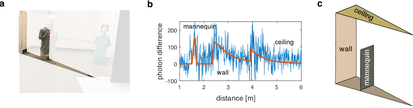
Figure 3: Reconstruction of a hidden wedge. a, A photograph of an example hidden scene, highlighting the wedge to be reconstructed. b, The proposed algorithm fits the planar facet model (orange) to the acquired histogram difference (blue), identifying contributions from the mannequin, wall, and ceiling. The time to each surface yields the position of the facets, the response shape provides information about the height and orientation, and the amplitude of the response is proportional to the surface albedo. c, This information is used to form a 2.5D reconstruction of the hidden wedge.

One major difficulty of NLOS imaging is that the number of surfaces per resolved wedge is unknown a priori and can vary across the hidden scene. Some wedges have only ceiling and wall contributions, whereas other wedges contain additional objects, such as the mannequins in our experiments. We simultaneously process all histogram differences to capture spatial dependencies between facet configurations across wedges of the hidden scene.

The performance of our reconstruction method relies on a carefully tailored scene model, which must be both flexible and informative while remaining computationally tractable. In natural hidden scenes, we observe that facets tend to be spatially clustered, with clusters representing different objects in the room. We also observe that the positions of facets belonging to the same object tend to describe a 1D manifold. For example, the walls of the room can be described by a concatenation of facets forming the perimeter of the hidden scene. Moreover, the parameters of neighbouring facets belonging to the same object are strongly correlated. For example, wall facets tend to share similar heights, albedos and orientations. These assumptions about scene structure are incorporated into the model via a Bayesian framework by defining a spatial point process prior model for the facet positions. This model is inspired by recent 3D reconstruction algorithms for LOS single-photon lidar that represent surfaces as 2D manifolds[28, 29]. Inference about the facet parameters (distance, height, albedo, and orientation angle) and the ceiling parameters (height and albedo) is carried out using a reversible-jump MCMC algorithm[30], which maximizes a posterior distribution to find the most likely hidden room configuration given the observed data and prior beliefs (see Supplementary Section 2). At each iteration, the algorithm proposes a random, yet guided, modification to the configuration of facets (e.g., addition or removal of a facet), which is accepted with a pre-defined rule (the Green ratio[30]). Note that this approach only requires the local evaluation of the forward model, i.e., for individual wedges, which takes advantage of the fast calculations based on Equation (0.2). In particular, we can efficiently take into account non-linear contributions due to occlusions between facets of a given wedge. By designing tailored updates (see Supplementary Section 2), the algorithm finds a good fit in few iterations, resulting in execution times of approximately 100 s, which is less than the acquisition time of the system.

0.4 Experimental Reconstructions.

Our reconstruction approach is assessed using measurements of challenging indoor scenes containing multiple objects with a variety of depths, heights, rotation angles, and albedos. The hidden scenes consist of an existing room structure modified by movable foamcore walls, with several objects placed within the scene. Black foamboard is used to create a vertical edge with reduced initial laser reflection intensity. Due to the specular nature of the existing floor, foamcore coated with a flat, white spray paint is used to achieve a more Lambertian illumination and detection relay surface, enabling even light distribution to all angles of the hidden scene.

Fig. 4 shows multiple views of the results of our reconstruction method for three example scenes.

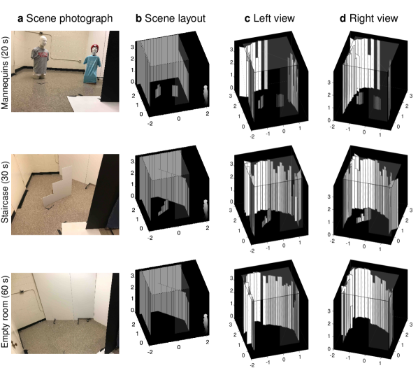
Figure 4: Reconstructions of hidden scenes. Acquisition times are shown in seconds per illumination spot, and distance measurements are in meters. a, Hidden scene photographs show rooms combining existing structures with moveable foamcore walls that are either empty or contain two mannequins or a planar staircase. b, Diagrams show the approximate layout of the hidden scene plus the position of an observer. c, Left & d, right views of the reconstructed scenes. The foreground objects are correctly localized with height estimates within $\approx$10 cm, and most of the wall components are recovered. The estimated ceiling height and the known occluder edge are shown with partial transparency for context.

Each dataset was acquired from 45 illumination positions, with acquisition times of 20 s per illuminated spot for the mannequins, 30 s per illuminated spot for the staircase, and 60 s per illuminated spot for the empty room. The approximate scene layout is displayed for reference using measurements from a laser distance meter. The foreground objects, the ceiling height, and most of the wall components are recovered, with visual inspection confirming approximately correct positions and orientations. The planar staircase object is useful as a height resolution test, with the average facet height for the 30-, 60-, and 90-cm steps measured to be 0.411, 0.543, and 0.921 m, respectively, yielding roughly 10-cm accuracy. The most challenging components to accurately recover are wall facets that are occluded, oblique-angled, and/or far from the vertical edge. Additional results varying the scene content, acquisition duration, and number of illumination spots are presented in the Supplementary Section 6.

In general, the histogram differences from real experimental data with reasonably short acquisition times are extremely noisy (see Fig. 3), which makes accurate estimation challenging. Situations in which the visible scene response is large, or there is significant ambient background light, result in high variance in the measurements. Furthermore, the variance in the measurements due to the hidden scene itself increases linearly as a function of the illumination angle $\theta$, making the estimation more difficult at higher angles. Despite these effects, our reconstruction approach is quite robust to low signal strength and a high number of background counts, as confirmed by additional simulations presented in the Supplementary Section 7.

Discussion

We have presented a method for imaging large-scale scenes outside the line of sight by measuring the transient light transport from scene illumination constrained by a visible occluder. Other time-resolved methods for NLOS imaging using a relay wall have ellipsoidal uncertainty in the position of a reflecting surface, requiring a large scan area with many illumination and/or detection points. The edge-resolving property of ERTI combined with the histogram differencing reduces the uncertainty from two dimensions to one, requiring dramatically fewer distinct measurements (e.g., 45 illumination locations) and a smaller aperture (e.g., 1.5 cm arc) than previous methods, as well as simplifying reconstruction. Moreover, existing methods using the floor as a relay surface depend on differences between multiple acquisitions to isolate 2D positions of moving objects from the “clutter” reflections from static surfaces[12], whereas ERTI recovers the entire static scene.

While we successfully demonstrate the ERTI acquisition and processing framework here, numerous aspects could be improved through updated experimental and modeling approaches. A straightforward method of decreasing the acquisition time would be to increase the laser power at the same wavelength[17, 18]. Other works have even shown promising results with linear-mode avalanche photodiodes and lasers at higher wavelengths with greater eye-safety[31]. Although we assume sequential illumination of evenly-spaced angles and a constant integration time for each spot, an alternative implementation could use a multi-resolution approach that first coarsely captures the hidden scene structure and then more finely samples areas that appear to have interesting content. Finally, ERTI opportunistically uses a vertical edge to recover directional information from the hidden scene, but other more complicated occluder shapes could be used in conjunction with modified modeling.

0.5 Experimental Setup.

A 120-mW master oscillator fiber amplifier (MOFA) picosecond laser (PicoQuant VisUV-532) at operating wavelength 532 nm is pulsed with repetition frequency $f_{\rm r}=$ 20 MHz. The illumination spot is redirected by a pair of galvo mirrors (Thorlabs GVS012), which is controlled by software through the analog outputs of a data acquisition (DAQ) interface (NI USB-6363). Simultaneously with the illumination trigger, the laser sends a synchronization signal to the TCSPC electronics (PicoQuant HydraHarp 400), which starts a timer. The “stop” signal for the timer is a detection event registered by the SPAD detector (Micro Photon Devices Fast-gated SPAD, photon detection efficiency $\approx$ 30% at 532 nm). These detection events may be due to true photon detections such as back-reflected signal or ambient light, or due to noise such as thermal dark counts or afterpulses.

The hardware is positioned approximately 2 m from the occluder edge. The laser illuminates a set of $n_{\ell}$ spots $\{\ell_{i}\}_{i=1}^{n_{\ell}}$ along a semicircle of radius $r_{\ell}$ on the floor plane, with the vertical edge at the center. The spots are linearly spaced in angle with $\ell_{1}$ at angle 0 completely occluded from the hidden scene, and $\ell_{n_{\ell}}$ at angle $\pi$ where none of the hidden scene is occluded.

The SPAD has a 25-mm lens mounted at the focal distance from the detector element, so that the SPAD field of view (FOV) is a small, approximately-circular spot of radius $r_{\rm o}$ on the ground plane. The SPAD is mounted on an articulating platform (Thorlabs SL20) and oriented so that the center of the FOV is approximately co-linear with the intersection of the ground plane and the occluding wall, a distance $r_{\rm s}\approx$ 20 cm from the corner. Mounted in front of the collection lens is a bandpass filter (Semrock MaxLine laser-line filter) with a transmission efficiency of $>90\%$ at the operating wavelength and a full width at half maximum (FWHM) bandwidth of 2 nm to reduce the amount of ambient light incident on the detector. The timing offset of the laser/SPAD system is adjusted such that round-trip time of flight to and from the corner spot is removed (i.e., the corner point is at time zero). Finally, a gate delay is adjusted so that the “first-bounce” light from the direct reflection is not recorded, to ensure that afterpulsing due to the strong direct reflection is minimized. The SPAD gating is controlled by a delayer unit (MPD Picosecond Delayer) to have a gate-on duration of 42 ns starting $\approx 3$ ns after the peak of the direct reflection.

The laser is directed by the galvos to illuminate each spot in sequence for a time $t_{\rm dwell}$ per spot. Detected photons are time-stamped by TCSPC module and streamed to the computer. When the DAQ changes the galvo voltages to change the coordinates of the laser position, it simultaneously sends a marker to the TCSPC module indicating the spot to which the subsequent detections belong. After the acquisition is completed, a histogram of detection times is formed for time bins with bin centers $\{b_{i}\}_{i=1}^{n_{\rm b}}$, where $n_{\rm b}=\lfloor t_{\rm r}/t_{\rm bin}\rfloor$ is the number of bins, $t_{\rm bin}$ is the bin resolution, and $t_{\rm r}=1/f_{\rm r}$ is the repetition period. In this way, histograms can be formed for any histogram dwell time $t_{\rm h}$, where $t_{\rm h}\in[0,t_{\rm dwell}]$.

References

We thank F. Durand, W. T. Freeman, J. H. Shapiro, A. Torralba, G. W. Wornell, and S. W. Seidel for discussions. This work was supported in part by the US Defense Advanced Research Projects Agency (DARPA) REVEAL Program under contract number HR0011-16-C-0030, in part by a Draper Fellowship under Navy contract N00030-16-C-0014, in part by the US National Science Foundation under grant number 1815896, in part by the Royal Academy of Engineering under the Research Fellowship scheme RF201617/16/31, in part by the Engineering and Physical Sciences Research Council (EPSRC) (grants EP/T00097X/1 and EP/S000631/1), and in part by the MOD University Defence Research Collaboration (UDRC) in Signal Processing.

References

- [1] Bouman, K. L. et al. Turning corners into cameras: Principles and methods. In Proc. IEEE Int. Conf. Comput. Vis., 2270–2278 (2017).
- [2] Baradad, M. et al. Inferring light fields from shadows. In Proc. IEEE Conf. Comput. Vis. Pattern Recog., 6267–6275 (2018).
- [3] Saunders, C., Murray-Bruce, J. & Goyal, V. K. Computational periscopy with an ordinary digital camera. Nature 565, 472 (2019).
- [4] Seidel, S. W. et al. Corner occluder computational periscopy: Estimating a hidden scene from a single photograph. In Proc. IEEE Int. Conf. Comput. Photogr., 25–33 (2019).
- [5] Yedidia, A. B., Baradad, M., Thrampoulidis, C., Freeman, W. T. & Wornell, G. W. Using unknown occluders to recover hidden scenes. In Proc. IEEE Conf. Comput. Vis. Pattern Recog., 12231–12239 (2019).
- [6] Thrampoulidis, C. et al. Exploiting occlusion in non-line-of-sight active imaging. IEEE Trans. Comput. Imaging 4, 419–431 (2018).
- [7] Xu, F. et al. Revealing hidden scenes by photon-efficient occlusion-based opportunistic active imaging. Opt. Expr. 49, 2259–2267 (2018).
- [8] Kirmani, A., Hutchison, T., Davis, J. & Raskar, R. Looking around the corner using transient imaging. In Proc. IEEE Int. Conf. Comput. Vis., 159–166 (2009).
- [9] Velten, A. et al. Recovering three-dimensional shape around a corner using ultrafast time-of-flight imaging. Nature Commun. 3, 745 (2012).
- [10] Heide, F., Xiao, L., Heidrich, W. & Hullin, M. B. Diffuse mirrors: 3D reconstruction from diffuse indirect illumination using inexpensive time-of-flight sensors. In Proc. IEEE Conf. Comput. Vis. Pattern Recog., 3222–3229 (2014).
- [11] Buttafava, M., Zeman, J., Tosi, A., Eliceiri, K. & Velten, A. Non-line-of-sight imaging using a time-gated single photon avalanche diode. Opt. Expr. 23 (2015).
- [12] Gariepy, G., Tonolini, F., Henderson, R., Leach, J. & Faccio, D. Detection and tracking of moving objects hidden from view. Nature Photon. 10, 23–26 (2016).
- [13] Pediredla, A. K., Buttafava, M., Tosi, A., Cossairt, O. & Veeraraghavan, A. Reconstructing rooms using photon echoes: A plane based model and reconstruction algorithm for looking around the corner. In Proc. IEEE Int. Conf. Comput. Photogr., 1–12 (2017).
- [14] O’Toole, M., Lindell, D. B. & Wetzstein, G. Confocal non-line-of-sight imaging based on the light-cone transform. Nature 25489 (2018).
- [15] Ahn, B., Dave, A., Veeraraghavan, A., Gkioulekas, I. & Sankaranarayanan, A. C. Convolutional approximations to the general non-line-of-sight imaging operator. In Proc. IEEE Int. Conf. Comput. Vis., 7889–7899 (2019).
- [16] Heide, F. et al. Non-line-of-sight imaging with partial occluders and surface normals. ACM Trans. Graph. 38, 1–10 (2019).
- [17] Lindell, D. B., Wetzstein, G. & O’Toole, M. Wave-based non-line-of-sight imaging using fast – migration. ACM Trans. Graph. 38, 116:1–116:13 (2019).
- [18] Liu, X. et al. Non-line-of-sight imaging using phasor-field virtual waveoptics. Nature 572, 620–623 (2019).
- [19] Pediredla, A., Dave, A. & Veeraraghavan, A. SNLOS: Non-line-of-sight scanning through temporal focusing. In Proc. IEEE Int. Conf. Comput. Photogr., 12–24 (2019).
- [20] Xin, S. et al. A theory of Fermat paths for non-line-of-sight shape reconstruction. In Proc. IEEE Conf. Comput. Vis. Pattern Recog. (2019).
- [21] Maeda, T., Wang, Y., Raskar, R. & Kadambi, A. Thermal non-line-of-sight imaging. In Proc. IEEE Int. Conf. Comput. Photogr., 1–11 (2019).
- [22] Lindell, D. B., Wetzstein, G. & Koltun, V. Acoustic non-line-of-sight imaging. In Proc. IEEE Conf. Comput. Vis. Pattern Recog. (2019).
- [23] Scheiner, N. et al. Seeing around street corners: Non-line-of-sight detection and tracking in-the-wild using Doppler radar. Preprint at http://arxiv.org/abs/1912.06613 (2019).
- [24] Torralba, A. & Freeman, W. T. Accidental pinhole and pinspeck cameras: Revealing the scene outside the picture. Int. J. Comput. Vis. 110, 92–112 (2014).
- [25] Brady, D. J., Pitsianis, N. P. & Sun, X. Reference structure tomography. J. Opt. Soc. Amer. A. 21, 1140 (2004).
- [26] Klein, J., Peters, C., Martín, J., Laurenzis, M. & Hullin, M. B. Tracking objects outside the line of sight using 2D intensity images. Sci. Rep. 6, 32491 (2016).
- [27] Skellam, J. G. The frequency distribution of the difference between two Poisson variates belonging to different populations. J. Roy. Statist. Soc. 109, 296 (1946).
- [28] Tachella, J. et al. Bayesian 3D reconstruction of complex scenes from single-photon lidar data. SIAM J. Imaging Sci. 12, 521–550 (2019).
- [29] Tachella, J. et al. Real-time 3D reconstruction from single-photon lidar data using plug-and-play point cloud denoisers. Nature Commun. 12, 4984 (2019).
- [30] Green, P. J. Reversible jump Markov chain Monte Carlo computation and Bayesian model determination. Biometrika 82, 711–732 (1995).
- [31] Brooks, J. & Faccio, D. A single-shot non-line-of-sight range-finder. Sensors 19 (2019).