Product Subset Problem : Applications to number theory and cryptography

Abstract.

We consider applications of Subset Product Problem (SPP) in number theory and cryptography. We obtain a probabilistic algorithm that solves SPP and we analyze it with respect time/space complexity and success probability. In fact we provide an application to the problem of finding Carmichael numbers and an attack to Naccache-Stern knapsack cryptosystem, where we update previous results.

1. Introduction

In the present paper we study the modular version of subset product problem (MSPP). This problem is defined in a similar way as the subset sum problem [10, 13]. We consider an application to number theory and cryptography. Furthermore, we shall provide an algorithm for solving MSPP based on birthday paradox attack. Finally we analyze the algorithm with respect to success probability and time/space complexity. Our applications concern the problem of finding Carmichael numbers and as far as the application on cryptography, we update previous results concerning an attack to the Naccache-Stern Knapsack (NSK) public key cryptosystem. We begin with the following definition.

Definition 1.1 (Subset Product Problem).

Given a list of integers $L$ and an integer $c$, find a subset of $L$ whose product is $c.$

This problem is (strong) NP-complete using a transformation from Exact Cover by 3-Sets (X3C) problem [14, p. 224], [41]. Also, see [12, Theorem 3.2], the authors proved that is at least as hard as Clique problem (with respect fixed-parameter tractability). In the present paper we consider the following variant.

Definition 1.2 (Modular Subset Product Problem : ${\rm MSPP}_{\Lambda}$).

Given a positive integer $\Lambda,$ an integer $c\in{\bf{Z}}_{\Lambda}^{*}$ and a vector $(u_{0},u_{1},...,u_{n})\in({\bf{Z}}_{\Lambda}^{*})^{n+1},$ find a binary vector $m=(m_{0},m_{1},...,m_{n})$ such that

(1.1) $$c\equiv\prod_{i=0}^{n}u_{i}^{m_{i}}\mod{\Lambda}.$$

The ${\rm{MSPP}_{\Lambda}}(\mathcal{P},c)$ problem can be defined also as follows : Given a finite set $\mathcal{P}\subset{\bf Z}_{\Lambda}^{*}$ and a number $c\in{\bf Z}_{\Lambda}^{*},$ find a subset $\mathcal{B}$ of $\mathcal{P},$ such that

$$\prod_{x\in{\mathcal{B}}}x\equiv c\mod\Lambda.$$

We can define MSPP for a general abelian finite group $G$ as following. We write $G$ multiplicative.

Definition 1.3 (Modular Subset Product Problem for $G$: ${\rm{MSPP}}_{G}({\mathcal{P}},c)$).

Given an element $c\in G$ and a vector $(u_{0},u_{1},...,u_{n})\in G^{n+1},$ find a binary vector $m=(m_{0},...,m_{n})$ such that,

(1.2) $$c=\prod_{i=0}^{n}u_{i}^{m_{i}}.$$

Although in the present work we are interested in $G={\bf{Z}}_{Q}^{*}$ where $Q$ is highly composite number (the case of Carmichael numbers) or prime (the case of NSK cryptosystem).

1.1. Our Contribution

First we provide an algorithm for solving product subset problem based on birthday paradox. This approach is not new, for instance see [31, Section 2.3]. Here we use a variant of [4, Section 3]. We study and implement a parallel version of this algorithm. This result to an improvement of the tables provided in [4]. Further, except the cryptanalysis of NSK cryptosystem, we applied our algorithm to the searching of Carmichael numbers. We used a method of Erdős, to the problem of finding Carmichael numbers with many prime divisors. We managed to generate a Carmichael number with $19589$ prime factors. Finally, we provide an abstract version of the algorithm in [4, Section 3], to the general product subset problem and further we analyze the algorithm as far as the selection of the parameters (this is provided in Proposition 3.6).

Roadmap. This paper is organized as follows. In section 2 we introduce the attack to MSPP based on birthday paradox. We further provide a detailed analysis. Section 4 is dedicated to applications. In subsection 4.1 we obtain an application of MSPP to Naccache-Stern Knapsack cryptosystem and in subsection 4.3 we provide some experimental results. Subsection 4.4 is dedicated to the problem of finding Carmichael numbers with many prime factors. We provide the necessary bibliography and known results. Finally, the last section contains some concluding remarks.

2. Birthday Attack to Modular Subset Product Problem

We call density of ${\rm{MSPP}_{G}}(\mathcal{P},c)$ the positive real number

$$d=\frac{|\mathcal{P}|}{\log_{2}{|G|}}.$$

If $G={\bf{Z}}_{\Lambda}^{*},$ then

$$d=\frac{|\mathcal{P}|}{\log_{2}{|{{\bf Z}_{\Lambda}^{*}}|}}=\frac{|\mathcal{P}|}{\log_{2}{\phi(\Lambda)}},$$

where $\phi$ is the Euler totient function. In a ${\rm{MSPP}_{G}}(\mathcal{P},c)$ having a large density, we expect to have many solutions.

A straightforward attack uses birthday paradox paradigm to ${\rm MSPP}_{\Lambda}(\mathcal{P},c)$. Rewriting equivalence (1.1) as

$$\prod_{i=0}^{\alpha}u_{i}^{m_{i}}\equiv c\prod_{i=\alpha+1}^{n}u_{i}^{-m_{i}}\mod{\Lambda},$$

for some integer $\alpha\approx n/2,$ we construct two subsets of ${\mathbb{Z}}_{\Lambda}$, say $U_{1}$ and $U_{2}.$ The first contains elements of the form $\prod_{i=0}^{\alpha}u_{i}^{m_{i}}\mod{\Lambda},$ and the second $c\prod_{i=\alpha+1}^{n}u_{i}^{-m_{i}}{\mod\Lambda},$ for all possible (binary) values of $\{m_{i}\}_{i}.$ So, the problem reduces to finding a common element of sets $U_{1}$ and $U_{2}.$ Below, we provide the pseudocode of the previous algorithm.

Algorithm 1: Birthday attack to ${\rm MSPP}_{\Lambda}\mathcal{(}\mathcal{P},c)$
INPUT : $\mathcal{P}=\{u_{i}\}_{i}\subset{\bf Z}_{\Lambda}^{*}$ $(|\mathcal{P}|=n+1),$ $c\in{\bf Z}_{\Lambda}^{*}$ (assume that $\gcd(u_{i},\Lambda)=1$)
OUTPUT: $\mathcal{B}\subset\mathcal{P}$ such that $\prod_{x\in{\mathcal{B}}}x\equiv c\mod{\Lambda}$ or Fail : There is not any solution

1: $I_{1}\leftarrow\{0,1,...,\lceil n/2\rceil\},I_{2}\leftarrow\{\lceil n/2\rceil+1,...,n\}$
2: $U_{1}\leftarrow\Big{\{}\prod_{i\in I_{1}}u_{i}^{\varepsilon_{i}}\mod\Lambda:\text{for \ all}\ \varepsilon_{i}\in\{0,1\}\Big{\}}$
3: $U_{2}\leftarrow\Big{\{}c\prod_{i\in I_{2}}u_{i}^{-\varepsilon_{i}}\mod\Lambda:\text{for \ all}\ \varepsilon_{i}\in\{0,1\}\Big{\}}$
4: If $U_{1}\cap U_{2}\not=\emptyset$
5:      Let $y$ be an element of $U_{1}\cap U_{2}$
6:      return $u_{i}:\prod u_{i}\equiv c\mod{\Lambda}.$
7: else return Fail : There is not any solution

This algorithm is deterministic, since if there is a solution to ${\rm MSPP}_{\Lambda}\mathcal{(}\mathcal{P},c)$ the algorithm will find it. To construct the solution in step 6, we use the equation

(2.1) $$\prod_{i\in I_{1}}u_{i}^{\varepsilon_{i}}=c\prod_{j\in I_{2}}u_{j}^{-\varepsilon_{j}}\ \ (\rm{in}\ \ {\bf Z}_{\Lambda}).$$

It turns out $y=\prod_{i=0}^{n}u_{i}^{\varepsilon_{i}}\mod{\Lambda}.$ For storage we need $2^{n/2+1}$ elements of ${\bf Z}_{\Lambda}^{*}.$ In line 4 we compute a common element. To do this we first sort the elements of $U_{1},U_{2}$ and then we apply binary search. Overall we need $O(2^{n/2}\log_{2}{n})$ arithmetic operations in the multiplicative group ${\bf Z}_{\Lambda}^{*}.$ The drawback of this algorithm is the large space complexity.

We can improve the previous algorithm as far as the space complexity.

3. An Improvement of Algorithm 2

We provide the following definitions.

Definition 3.1.

Let $c\in{\bf{Z}}_{\Lambda}^{*}$. We define

$${\rm{sol}}(c;{\mathcal{P}},\Lambda)=\{I\subset\{0,1,...,n\}:c\equiv\prod_{i\in I,\ u_{i}\in\mathcal{P}}u_{i}\mod\Lambda\}.$$

Let the map,

$$\chi:{\rm{sol}}(c;{\mathcal{P}},\Lambda)\rightarrow\{0,1\}^{n+1},$$

such that $\chi(I)=(\varepsilon_{0},\varepsilon_{1},...,\varepsilon_{n}),$ where $\varepsilon_{i}=1$ if $i\in I$ else $\varepsilon_{i}=0.$

Definition 3.2.

We define,

$${\rm{Sol}}(c;{\mathcal{P}},\Lambda)=\{(u_{0}^{\varepsilon_{0}},u_{1}^{\varepsilon_{1}},...,u_{n}^{\varepsilon_{n}}):\chi(I)=(\varepsilon_{0},\varepsilon_{1},...,\varepsilon_{n})\ \text{for\ all}\ I\in{\rm{sol}}(c;{\mathcal{P}},\Lambda)\}.$$

Definition 3.3.

To each element $I$ of ${\rm{sol}}(c;\mathcal{P},\Lambda)$ (assuming there exists one) we correspond the natural number $H_{I}(c)=|I|$ (the cardinality of $I$). We call this number local Hamming weight of $c$ at $I.$ We call Hamming weight $H(c)$ of $c,$ the minimum of all these numbers. I.e.

$$H(c)=\min\{H_{I}(c):I\in{\rm{Sol}}(c;{\mathcal{P}},\Lambda)\}.$$

Remark that the local Hamming weight of $c$ at $I$ is in fact the Hamming weight of the binary vector $\chi(I).$ That is, the sum of all the entries of $\chi(I).$ Thus,

$$H_{I}(c)=\sum_{i=0}^{n}\varepsilon_{i},{\rm{where}}\ \chi(I)=(\varepsilon_{0},\varepsilon_{1},...,\varepsilon_{n}).$$

Example 3.4.

Let $\mathcal{P}=\{2,3,...,10^{7}\},$ $\Lambda=10000019,$ $c=190238.$ There is an element $\Sigma$ of ${\rm{Sol}}(c;{\mathcal{P}},\Lambda),$

$$\Sigma=(9851537,303860,4680021,9647209,2006838,9984877,$$

$$2512434,2126904,1942182,8985302,2193757).$$

Note that we have trimmed all the ones. I.e.

$$\Sigma^{\prime}=(1,..,1,303860,1,...,1942182,1,...,9984877,1...,1).$$

Straightforward calculations provide,

$$\prod_{x\in\Sigma}x=\prod_{x\in\Sigma^{\prime}}x\equiv 190238=c\pmod{\Lambda}.$$

Also there is an element in ${\rm{sol}}(c;{\mathcal{P}},\Lambda)$ say $I,$ such that,

$$\chi(I)=\Sigma^{\prime}.$$

So in this case the local hamming weight of $c$ at $I$ is $11.$ However, the computation of the hamming weight of $c$ is more difficult. Note that $H(c)\geq 2,$ except if some $u_{i}$ is equal to $c.$ We do not consider this trivial case. For now, we can only say that $H(c)\leq 11.$ I.e. every local Hamming weight is an upper bound for $H(c).$

Now, let $I\in{\rm{sol}}(c;{\mathcal{P}},\Lambda).$ We consider two positive integers, say $h_{1},h_{2},$ such that, $h_{1}+h_{2}=H_{I}(c),$ and two disjoint subsets $I_{1},\ I_{2}$ of $\{0,1,\dots,n\}$ with $|I_{1}|=|I_{2}|=b,$ for some positive integer $b\leq n/2.$ Finally, we consider the sets,

$$U_{h_{1}}(I_{1};\mathcal{P},\Lambda)=\Big{\{}\prod_{i\in I_{1}}u_{i}^{\varepsilon_{i}}\pmod{\Lambda}:\sum_{i\in I_{1}}\varepsilon_{i}=h_{1}\Big{\}},$$

$$U_{h_{2}}(I_{2},c;\mathcal{P},\Lambda)=\Big{\{}c\prod_{i\in I_{2}}u_{i}^{-\varepsilon_{i}}\pmod{\Lambda}:\sum_{i\in I_{2}}\varepsilon_{i}=h_{2}\Big{\}}.$$

We usually write them as $U_{h_{1}}(I_{1})$ and $U_{h_{2}}(I_{2},c)$ since $\mathcal{P}$ and $\Lambda$ are known. We have,

$$|U_{h_{1}}(I_{1})|=\binom{|I_{1}|}{h_{1}},\ |U_{h_{2}}(I_{2},c)|=\binom{|I_{2}|}{h_{2}}.$$

Remark 3.1.

The set $U_{1}$ of Algorithm 2 is written,

$$U_{1}=\bigcup_{h_{1}=1}^{\lceil n/2\rceil+1}U_{h_{1}}(\{0,1,\dots,\lceil n/2\rceil\};\mathcal{P},\Lambda).$$

I.e. $U_{1}$ is the union of the sets $\{U_{h}(I;\mathcal{P},\Lambda)\}_{1\leq h\leq\lceil n/2\rceil+1}$ for $I=\{0,1,...,\lceil n/2\rceil\}.$ Similar $U_{2}$ is written,

$$U_{2}=\bigcup_{h_{2}=0}^{n-\lceil\frac{n}{2}\rceil}U_{h_{2}}(\{\lceil n/2\rceil+1,...,n\},c;\mathcal{P},\Lambda).$$

Instead of using $U_{1},U_{2}$ we use subsets of them. The choice of subsets creates a probability distribution at the output. So this choice must be studied as fas as the success probability. For the following algorithm we assume that we know a local Hamming weight of the target number $c.$ 

Algorithm 2 ${\rm BA\_MSPP}_{\Lambda}({\mathcal{P}},c;b,\ell,Q,{\rm iter})$ : Memory efficient attack to ${\rm MSPP}_{\Lambda}(\mathcal{P},c)$
INPUT:
${\bf i}.$ A set $\mathcal{P}=\{u_{i}\}_{i}\subset{\bf Z}_{\Lambda}^{*}$ with $|\mathcal{P}|=n+1$ (assume that $\gcd(u_{i},\Lambda)=1$)
${\bf ii}.$ a number $c\in{\bf Z}_{\Lambda}^{*}$
${\bf iii}.$ a local Hamming weight of $c,$ say $\ell$
${\bf iv}.$ a positive number $b:$ $\ell\leq b\leq n/2$
${\bf v}.$ a compression function ${\mathbb{H}}$
${\bf vi}.$ a positive integer iter

OUTPUT: a set $\mathcal{B}\subset\mathcal{P},$ such that $\prod_{x\in{\mathcal{B}}}x\equiv c\mod{\Lambda}$ or Fail

1: $(h_{1},h_{2})\leftarrow(\lfloor\ell/2\rfloor,\lceil\ell/2\rceil)$
2: For $i$ in $1,\dots,iter$
3:       $(I_{1},I_{2})\xleftarrow{\$}\{0,...,n\}\times\{0,...,n\}$  # with $I_{1},I_{2}$ disjoint and $|I_{1}|=|I_{2}|=b$
4:      $U_{h_{1}}^{*}(I_{1})\leftarrow\Big{\{}{\mathbb{H}}\big{(}\prod_{i\in I_{1}}u_{i}^{\varepsilon_{i}}\pmod{\Lambda}\big{)}:\sum_{i\in I_{1}}\varepsilon_{i}=h_{1},\ \varepsilon_{i}\in\{0,1\}\Big{\}}$
5:      For each $(\varepsilon_{i})_{i}$ such that $:\sum_{i\in I_{2}}\varepsilon_{i}=h_{2}$
6:         If  ${\mathbb{H}}\big{(}c\prod_{i\in I_{2}}u_{i}^{-\varepsilon_{i}}\pmod{\Lambda}\big{)}\in U_{h_{1}}^{*}(I_{1})$
7:             Let $y$ be an element of $U_{h_{1}}^{*}(I_{1})\cap U_{h_{2}}^{*}(I_{2},c)$
8:             return $\{u_{i}\}_{i}$ such that $\prod u_{i}\equiv c\mod{\Lambda}$ and terminate
9: return Fail # if for all the iterations the algorithm failed to find a solution

This algorithm is a memory efficient version of algorithm 2, since we consider subsets of $U_{1},U_{2}.$ Although, this algorithm may fail, even when ${\rm MSPP}_{\Lambda}(\mathcal{P},c)$ has a solution. For instance, assuming that ${\rm{sol}}(c;\mathcal{P},\Lambda)\not=\emptyset,$ if we pick $I_{1},I_{2}$ and happens that the union $I_{1}\cup I_{2}\not\in{\rm{sol}}(c;\mathcal{P},\Lambda),$ then the algorithm will fail. I.e. the problem may have a solution but the algorithm failed to find it. This may occur when $b<n/2,$ that is $I_{1}\cup I_{2}\subset\{0,1,...,n\}.$ If $I_{1}\cup I_{2}=\{0,1,...,n\},$ then the algorithm remains probabilistic, since we consider a specific choice of $(h_{1},h_{2})$ and not all the possible $(h_{1},h_{2}),$ with $h_{1}+h_{2}=\ell.$ If we consider all $(h_{1},h_{2})$ such that $h_{1}+h_{2}=n,$ then the algorithm turns out to be deterministic.

We analyze the algorithm line by line.
Line 3: This can be implemented easily in the case where $2b<\sqrt{n}.$ Indeed, we can use rejection sampling in the set $\{0,...,n\}$ and construct a list of length $2b.$ Then, $I_{1}$ is the set consisting from the first $b$ elements and $I_{2}$ the rest. If $2b\geq\sqrt{n}$ then, we have to sample from the set $\{0,1,...,n\},$ so the memory increases since we have to store the set $\{0,1,...,n\}.$ For instance, when we apply the algorithm to the searching of Carmichael numbers we have $2b\ll\sqrt{n}.$ In the case of NSK cryptosystem we usually have $2b>\sqrt{n}.$
Line 4: The most intensive part (both for memory and time complexity) is the construction of the set $U_{h_{1}}^{*}$. Here we can parallelize our algorithm to decrease time complexity. To reduce the space complexity we use the parameter $b\leq n/2$ and the compression function ${\mathbb{H}}.$ For instance as a a compression function we consider $Q-$ strings of the output of a hash function. We consider that the output of the hash function is a hex string. In subsection 3.4 we provide a strategy to choose $Q.$
Line 5-6: In Line 4 we stored $U_{h_{1}}^{*}(I_{1}),$ in this line we compute on the fly the elements of the second set $U_{h_{2}}^{*}(I_{2},c)$ and check if any is in $U_{h_{1}}^{*}(I_{1}).$ So we do not need to store $U_{h_{2}}^{*}.$ A suitable data structure for the searching is the hashtable, which we also used in our implementation. Hashtables have the advantage of the fast insert, delete and search operations. Since these operations have $O(1)$ time complexity on the average.
Line 7-8: Having the element found by the previous step (Line 6), say $y,$ we construct the $u_{i}$’s such that their product is $y.$ We return Fail if the intersection is empty for all the iterations.

Remark 3.2.

If we do not consider any hash function and ${\rm iter}=1,$ then we write ${\rm BA\_MSPP}_{\Lambda}({\mathcal{P}},c;b,\ell).$

3.1. Space complexity

We assume that there is not any collision in the construction of $U_{h_{1}}^{*}(I_{1})$ and $U_{h_{2}}^{*}(I_{2},c),$ or in other words we choose $Q$ to minimize the probability to have a collision. I.e. we choose $2^{4Q}\gg\max\{|U_{1}|,|U_{2}|\}$ and we assume that ${\mathbb{H}}$ is behaving random enough. In practice (or at least in our examples) we always have this constraint.

So we get,

$$|U_{h_{1}}(I_{1})|=|U_{h_{1}}^{*}(I_{1})|=\binom{|I_{1}|}{h_{1}}\ \text{ and}\ \ |U_{h_{2}}(I_{2},c)|=|U_{h_{2}}^{*}(I_{2},c)|=\binom{|I_{2}|}{h_{2}},$$

where $(h_{1},h_{2})=(\lfloor\ell/2\rfloor,\lceil\ell/2\rceil).$ By choosing $|I_{1}|=|I_{2}|=b,$ we get

$$|U_{h_{1}}^{*}(I_{1})|=\binom{b}{h_{1}}\ \ \text{and}\ \ |U_{h_{2}}^{*}(I_{2},c)|=\binom{b}{h_{2}}.$$

We set

$$S_{b}=\binom{b}{h_{1}}=B_{b}(h_{1}).$$

In our algorithm, we need to store the $S_{b}$ hashes of the set $U_{h_{1}}^{*}(I_{1}).$ We need $4Q-$bits for keeping $Q-$hex digits in the memory. So, overall we store $4QS_{b}$ bits. Furthermore, we store the binary exponents $(\varepsilon_{i})_{i}$ that are necessary for the computation of the products, $\prod_{i\in I_{1}}u_{i}^{\varepsilon_{i}}.$ This is needed, since we must reconstruct $c$ as a product of $(u_{i})_{i}.$ These are $S_{b},$ thus we need $b\times S_{b}-$ bits. Since we also need to store the set $\mathcal{P}$ of length $n+1,$ we conclude that,

(3.1) $$\mathbb{M}<(4Q+b)S_{b}+(n+1)B\ \ (\text{bits}),$$

where $B=\max\{\log_{2}(x):x\in\mathcal{P}\}.$ Remark that ${\mathbb{M}}$ does not depend on the modulus $\Lambda.$

$\ell$	9	11	13	15	17	19	21
${\mathbb{M}}\ (GB)$	0.029	0.05	0.2	1.16	6.15	28.61	117.2

Table 1. For $b=50,\ Q=12$ and $\mathcal{P}=\{2,3,...,10^{7}\}$.

If we can describe in an efficient way the set $\mathcal{P}$ we do not need to store it. Say, that $\mathcal{P}=\{2,3,...,n\}.$ Then, there is no need to store it in the memory, since the sequence $f(x)=x+1$ describes efficiently the set $\mathcal{P}.$ Also, in other situations $B$ can be stored using $O(|{\mathcal{P}}|\log_{2}(|{\mathcal{P}}|))$ bits. We call such sets nice and they can save us enough memory. In fact, for nice sets the inequality (3.1) changes to,

(3.2) $$\mathbb{M}<(4Q+b)S_{b}+O(n\log_{2}n)\ \ (\text{bits}).$$

In fact when we apply this algorithm to the problem of finding Carmichael numbers, we shall see that the set $\mathcal{P}$ is nice.

Finally, if $U_{h_{1}}$ is very large we can make chunks of it, to store it in the memory. Note that this can not be done if we directly compute the intersection of $U_{h_{1}}\cap U_{h_{2}}$ as in [4]. This simple trick considerable improves the algorithms in [4].

3.2. Time complexity

Time complexity is dominated by the construction of the sets $U_{h_{1}}$ and $U_{h_{2}}$ and the calculation of their intersection. We work with $U_{h_{1}}$ instead of $U_{h_{1}}^{*}$ since all the multiplications are between the elements of $U_{h_{1}}$, only in the searching phase we move to $U_{h_{1}}^{*}$. Let $M_{\Lambda}$ be the bit-complexity of the multiplication of two integers $\mod\Lambda.$ So

$$M_{\Lambda}=O((\log_{2}{\Lambda})^{1+\varepsilon})$$

for some $0<\varepsilon\leq 1$ (for instance Karatsuba suggests $\varepsilon=\log_{2}{3}-1$ [21]). In fact recently was proved $M_{\Lambda}=O(\log_{2}{\Lambda}\log_{2}{(\log_{2}{\Lambda}}))$ [18]. To construct the sets $U_{h_{1}}$ and $U_{h_{2}}$ (ignoring the cost for the inversion ${\mod\Lambda}$) we need $M_{\Lambda}h_{1}B_{b}(h_{1})=M_{\Lambda}h_{1}S_{b}$ bit-operations for the set $U_{h_{1}}$ and $M_{\Lambda}h_{2}B_{b}(h_{2}+1)\approx M_{\Lambda}h_{2}S_{b}$ bit-operations for $U_{h_{2}}.$ So overall,

$${\mathbb{T}}_{1}=M_{\Lambda}(h_{1}S_{b}+h_{2}S_{b})=M_{\Lambda}S_{b}(h_{1}+h_{2})\ \text{bits}.$$

Considering the time complexity for finding a collision in the two sets by using a hashtable, we get

$${\mathbb{T}}={\mathbb{T}}_{1}+O(1)S_{b}\ \text{bits}\ \text{on\ average}$$

and

$${\mathbb{T}}={\mathbb{T}}_{1}+O(1)S_{b}^{2}\ \text{in\ the\ worst\ case}.$$

We used that $h_{1}\approx h_{2}$ (they differ at most by $1$). In case we have $T$ threads we get about ${\mathbb{T}}/T$ (bit operations) instead of ${\mathbb{T}}.$

3.3. Success Probability

In the following Lemma we compute the probability to get a common element in $U_{h_{1}}(I_{1})$ and $U_{h_{2}}(I_{2},c)$ when $(I_{1},I_{2})\xleftarrow{\$}\{0,...,n\}\times\{0,...,n\},$ where $I_{1},I_{2}$ are disjoint, with $b$ elements. Let $0\leq y\leq x.$ With $B_{x}(y)$ we denote the binomial coefficient $\binom{x}{y}.$

Lemma 3.5.

Let $h_{1},h_{2}$ be positive integers and $\ell=h_{1}+h_{2}.$ The probability to get $U_{h_{1}}(I_{1})\cap U_{h_{2}}(I_{2},c)\not=\emptyset$ is,

$${\mathbb{P}}=\frac{B_{b}(h_{1})B_{b}(h_{2})}{B_{n+1}(\ell)}.$$

For the proof see [4, section 3].

We can easily provide another and simpler proof in the case $2b=n+1$ (this occurs very often when attacking Naccache-Stern cryptosystem). Then,

$${\mathbb{P}}=hyper(x;2b,b,\ell),$$

where hyper is the hypergeometric distribution,

$$hyper(x;N,b,\ell)=Pr(X=x)=\frac{\binom{b}{x}\binom{N-b}{\ell-x}}{\binom{N}{\ell}}.$$

Where,
$\bullet$ $N=n+1$ is the population size
$\bullet$ $\ell$ is the number of draws
$\bullet$ $b$ is the number of successes in the population
$\bullet$ $x$ is the number of observed successes
Adapting to our case, we set $N=2b=n+1,\ell=h_{1}+h_{2},$ and $x=h_{1}.$ Then,

$$hyper(x=h_{1};n+1,b,\ell)=Pr(X=h_{1})=\frac{\binom{b}{h_{1}}\binom{b}{\ell-h_{1}}}{\binom{n+1}{\ell}}=\mathbb{P}.$$

The expected value is $\frac{b\ell}{n+1}$ and since $b=(n+1)/2$ we get $EX=\frac{\ell}{2}.$ Since the random variable $X$ counts the successes we expect on average to have $\ell/2$ after considering enough instances (i.e. choices of $I_{1},$ $I_{2}$). The maximum value of $\ell$ is $n/2.$ Thus, in this case the expected value is maximized, hence we expect our algorithm to find faster a solution from another one that uses smaller value for $\ell.$

Also, we need about

$$\frac{1}{{\mathbb{P}}}=\frac{\binom{n+1}{\ell}}{\binom{b}{h_{1}}\binom{b}{h_{2}}}\ \text{iterations on average to find a solution}.$$

One last remark is that the contribution of $b$ is bigger than the contribution of hamming weight in the probability ${\mathbb{P}}.$

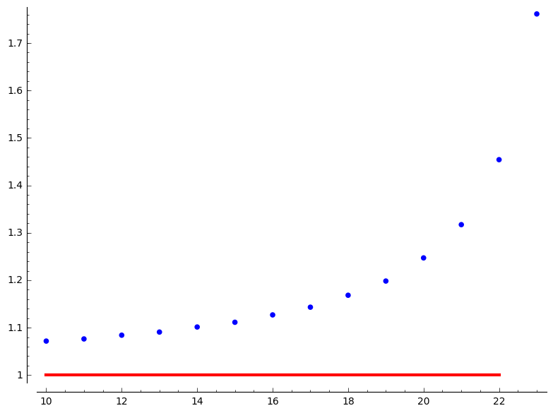
Figure 1. We fixed $n=23000$ and $b=35.$ We consider pairs $(h,f(h)),$ where $f(h)=\big{(}{\mathbb{P}(b+1,h)}/{\mathbb{P}(b,h+1)}\big{)}$ and $h$ the hamming weight. We finally normalized the values by taking logarithms. So, for a given $(b,h),$ if we want to increase the probability is better strategy to increase $b$ than $h.$

3.3.1. The best choice of $h_{1}$ and $h_{2}$

The choice of $h_{1},h_{2}$ (in line 1 of algorithm 3) is $h_{1}=\lfloor\ell/2\rfloor,$ $h_{2}=\lceil\ell/2\rceil.$ This can be explained easily, since these values maximize the probability ${\mathbb{P}}$ of Lemma 3.5. We set

$$J_{\ell}=\{(x,y)\in{\bf{Z}}^{2}:x+y=\ell,0\leq x\leq y\}.$$

Observe that $(\lfloor\ell/2\rfloor,\lceil\ell/2\rceil)\in J_{\ell}.$

Proposition 3.6.

Let $b$ and $n$ be fixed positive integers such that $\ell=x+y\leq b\leq n/2.$ Then the finite sequence ${\mathbb{P}}:J_{\ell}\rightarrow{\mathbb{Q}},$ defined by

$${\mathbb{P}}(x,y)=\frac{B_{b}(x)B_{b}(y)}{B_{n+1}(\ell)},$$

is maximized for $(x,y)=(\lfloor\ell/2\rfloor,\lceil\ell/2\rceil).$

We need the following simple lemma.

Lemma 3.7.

$$\binom{b}{x}\binom{b}{\ell-x}\binom{2b}{b}=\binom{\ell}{x}\binom{2b-\ell}{b-x}\binom{2b}{\ell}.$$

Proof.

It is straightforward by expressing the binomial coefficients in terms of factorials and rearranging them. ∎

Proof of Proposition 3.6.

From the previous lemma we have

(3.3) $$\frac{\binom{b}{x}\binom{b}{\ell-x}}{\binom{2b}{\ell}}=\frac{\binom{\ell}{x}\binom{2b-\ell}{b-x}}{\binom{2b}{b}}.$$

Since $b,\ell$ are fixed, the maximum of the right hand side is at $x=\lfloor\ell/2\rfloor$. Indeed, both sequences $\binom{b}{x}$ and $\binom{2b-\ell}{b-x}$ are positive and maximized at $x=\lfloor\ell/2\rfloor.$ So also the product $\binom{\ell}{x}\binom{2b-\ell}{b-x}$ is maximized at $x=\lfloor\ell/2\rfloor.$ The same occurs to the left hand side. Since the denominator of the left hand side in (3.3) is fixed, the numerator $B_{b}(x)B_{b}(\ell-x)=\binom{b}{x}\binom{b}{\ell-x}$ is maximized at $x=\lfloor\ell/2\rfloor.$ Since $n$ is also a fixed positive integer, the numerator of ${\mathbb{P}}$ is maximized at $x=\lfloor\ell/2\rfloor$ and so ${\mathbb{P}}$ is maximized at the same point. Finally, $\ell-\lfloor\ell/2\rfloor=\lceil\ell/2\rceil=y.$ The Proposition follows. ∎

3.4. How to choose $Q?$

If we are searching for $r-$same objects to one set (with cardinality $n$), when we pick the elements of the set from some largest set (with cardinality $m$), then we say that we have a $r-$multicollision. We have the following Lemma.

Lemma 3.8.

If we have a set with $m$ elements and we pick randomly (and independently) $n$ elements from the set, then the expected number of $r-$mullticolisions is approximately

(3.4) $$\frac{n^{r}}{r!m^{r-1}}.$$

Proof.

[20, section 6.2.1] ∎

Say we use md5 hash function. If we use the parameter $Q$, we have to truncate the output of md5, which has $16-$hex strings, to $Q-$hex strings ($Q<16$). I.e we only consider the first $\kappa=4\cdot Q$-bits of the output. Our strategy to choose $Q$ uses formula (3.4). In practice, is enough to avoid $r=3-$multicollisions in the set $U_{h_{1}}^{*}(I_{1})\cup U_{h_{2}}^{*}(I_{2},c)$ of cardinality $S_{b},$ where

$$S_{b}=|U_{h_{1}}^{*}(I_{1})\cup U_{h_{2}}^{*}(I_{2},c)|=\binom{|I_{1}|}{h_{1}}+\binom{|I_{1}|}{h_{2}}.$$

We set the formula (3.4) equal to 1 and we solve with respect to $m$, which in our case is $m=2^{\kappa}.$ So, $\frac{S_{b}^{3}}{6}=2^{2\kappa}.$ Therefore we get, $\kappa\approx(3\log_{2}{S_{b}})/2$ (since in our examples $\log_{2}(S_{b})\gg\log_{2}{6}).$ For instance if we have local Hamming weight $\leq 13,$ $b=n/2,$ $|I_{1}|=|I_{2}|=b,$ and $n=232,$ we get $\kappa\approx 52.$ So, $Q\approx 13.$ In fact we used $Q=12$ in our attack to Naccache-Stern knapsack cryptosystem.

4. Applications

4.1. Naccache-Stern Knapsack Cryptosystem

In this section we consider a second application of MSPP to cryptography. We shall provide an attack to a public key cryptosystem. Naccache-Stern Knapsack (NSK) cryptosystem is a public key cryptosystem ([31]) based on the Discrete Logarithm Problem (DLP), which is a difficult number theory problem. Furthermore, it is based on another combinatorial problem, the Modular Subset Product Problem. Our attack applies to the latter problem. NSK cryptosystem is defined by the following three algorithms.

i. Key Generation:
Let $p$ be a large safe prime number (that is $(p-1)/2$ is a prime number). Let $n$ denotes the largest positive integer such that:

(4.1) $$p>\prod_{i=0}^{n}p_{i},$$

where $p_{i}$ is the $(i+1)-$th prime. The message space of the system is $\mathcal{M}=\{0,1\}^{n+1},$ this is the set of the binary strings of $(n+1)-$bits. For instance, if $p$ has $2048$ bits, then $n=232$ and if $p$ has $1024$ bits, then $n=130.$

We randomly pick a positive integer $s<p-1$, such that $\gcd(s,p-1)=1$. This last property guarantees that there exists the (unique) $s-$th root $\mod{p}$ of an element in ${\bf Z}_{p}^{*}.$ Set

$$u_{i}=\sqrt[s]{p_{i}}\mod{p}\in{\bf{Z}}_{p}^{*}.$$

The public key is the vector

$$(p,n;u_{0},...,u_{n})\in{\bf{Z}}^{2}\times({\bf{Z}}_{p}^{*})^{n+1}$$

and the secret key is $s$.

ii. Encryption:
Let $m$ be a message and $\sum_{i=0}^{n}2^{i}m_{i}$ its binary expansion. The encryption of the $n+1$ bit message $m$ is $c=\prod_{i=0}^{n}u_{i}^{m_{i}}\mod{p}$.
iii. Decryption:
To decrypt the ciphertext $c,$ we compute

$$m=\sum_{i=0}^{n}\frac{2^{i}}{p_{i}-1}\times\big{(}\gcd(p_{i},c^{s}\mod{p})-1\big{)}.$$

From the description of the NSK scheme, we see that the security is based on the Discrete Logarithm Problem (DLP). It is sufficient to solve $u_{i}^{x}=p_{i}$ in ${\bf Z}_{p}^{*},$ for some $i.$ The best algorithm for computing DLP in prime fields has subexponential bit complexity, [1, 15]. Thus, for large $p$ (at least $2048$ bits) the system can not be attacked by using the state of the art algorithms for DLP.

We have also assumed that the prime number $p$ belongs to the special class of safe primes to prevent attacks such as, Pollard rho [35], Pollard $p-1$ algorithm [34], Pohlig-Hellman algorithm [33] or any similar procedure that exploits properties of $p-1.$

4.2. The attack

Since, $c\equiv\sum_{i=0}^{n}2^{i}m_{i}\mod{\Lambda},$ we get

(4.2) $$\prod_{i\in I_{1}}u_{i}^{m_{i}}=c\prod_{i\in I_{2}}u_{i}^{-m_{i}}\ \ (\rm{in}\ \ {\bf Z}_{\Lambda}).$$

So we can apply ${\rm BA\_MSPP}_{\Lambda}$ with input ${\mathcal{P}}=(u_{i})_{i}$ and $c$ and for some bound $b$ and hamming weight of the message $m$ say $H_{m}$ i.e. the number of $1^{\prime}$s in the binary message $m.$ So in this attack we assume that we know the hamming weight or an upper bound of it. To be more precise, this attack is feasible only for small or large hamming weights. Our parallel version allow us to consider larger hamming weights than in [4].

In the following algorithm we call algorithm 3, where we execute steps 4 and 5 in parallel (in function ${\rm BA\_MSPP}_{\Lambda}$).  

Algorithm 3 : Attack to NSK cryptosystem
INPUT: $\circ$ The cryptographic message $c$
$\circ$ the Hamming weight $H_{m}$ of the message $m$
$\circ$ a bound $b\leq n/2$
$\circ$ the public key $pk=(p,n;u_{0},...,u_{n})$ of NSK cryptosystem

OUTPUT: the message $m$ or Fail

1: ${\mathcal{P}}\leftarrow\{u_{0},...,u_{n}\}$
2: ${\mathbb{S}}\leftarrow{\rm{BA\_MSPP}}_{p}({\mathcal{P},c;b,H_{m}})$
3: if ${\mathbb{S}}\not=\emptyset$ construct $m.$ Else return Fail

4.2.1. Reduction of the case of large Hamming weight messages

The case where we have large Hamming weight of a message can be reduced to the case where we have small Hamming weight. Indeed, if the message $m$ has $H_{m}=n+1-\varepsilon,$ where $\varepsilon$ is a small positive integer, then again we can reduce the problem to one with small Hamming weight. Let $c=Enc(m)$ and $c^{\prime}=c^{-1}u_{n}^{2}\prod_{i=0}^{n-1}u_{i}.$ We provide the following Lemma.

Lemma 4.1.

The decryption of $c^{\prime}$ is $m^{\prime}=2^{n+1}+2^{n}-m-1,$ where $H_{m^{\prime}}=\varepsilon+1.$

Proof.

[4, Lemma 3.4] ∎

So we can consider $H_{m}<b.$ Indeed, if $H_{m}\geq b,$ we apply the previous Lemma and we get $H_{m^{\prime}}<b.$ So finding $m^{\prime}$ is equivalent finding $m.$

4.2.2. The case of knowing some bits of the message

If we know the position of some bits of the message $m$ (for instance by applying a fault attack to the system may leak some bits), then we can improve our attack. In this case, we choose $I_{1}$ and $I_{2}$ in algorithm 4.2, from the set $\{0,1,..,n\}-K,$ where the set $K$ contains the positions of the known bits. Also, in line 10, when we reconstruct the message $m$ (in case of a collision) we need to put the known bits to the right positions.

4.3. Experimental results for NSK cryptosystem

In our implementation we used C/C++ with GMP library [17] and for parallelization OpenMP [32]. We used $20$ threads of an Intel(R) Xeon(R) CPU E5-2630 v4 $@2.20GHz,$ in a Linux platform.

First, in table 2 we present the improvement of the results provided in [4] by using the parallel version. Besides, in table 3 we extend the results of the previous table. In fact, table 3 demonstrates that having a suitable number of threads and considering a suitable bound $b$ we get a practical attack for low Hamming weight messages. In figure 2 we represent some of our data graphically.

${\rm len}(p)$		$600$			$1024$		$2048$
$H_{m}$	8	9	10	8	9	10	7	8
Attack [4]	$42$s	$300$s	$7.5$m	$8.1$m	$1.1$h	$1.96$h	$1.17$h	$2.15$h
Parallel Attack	$<1$s	$6.54$s	$15.56$s	$11.44$s	$70$s	$284$s	$70$s	$11.46$m

Table 2. We used $b=n/2,Q=12,$ where $n=84,130$ and $232,$ for ${\rm{len}}(p)=600,1024$ and $2048$ bits, respectively. For each column, we executed $10$ times the attack of [4] and our parallel version (algorithm 4.2), and we computed the average CPU time.

${\rm len}(p)$		$600$			$1024$			$2048$
$n$		$84$			$130$			$232$
$H_{m}$	12	13	14	11	12	13	9	10	11
Parallel (time)	$4$m	$7$m	$13$m	$26$m	$66$m	$142$m	$52$m	$107$m	$895$m
Mem. (GB)	1.43	4.93	7.5	14.28	21.67	67.41	26.9	40.61	127.53
Average Rounds	4.2	2.4	2.6	8.2	2.6	5.6	7.4	2.4	10

Table 3. Extension of table 2. For the case $H_{m}=13,\ Q=12,$ and ${\rm{len}}(p)=1024$ we used $b=60$ instead of $b=\frac{n}{2}=65.$ For the case $H_{m}=11$ and ${\rm{len}}(p)=2048$ we used $b=n/2-23=93.$ For all other cases we used $b=\frac{n}{2}.$ The last row, Average Rounds, is the (average) round that eventually our algorithm terminates. Theoretically is approximately $\frac{1}{{\mathbb{P}}}$ (see Lemma 3.5).

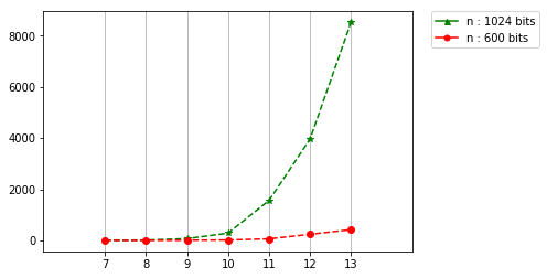
Figure 2. The horizontal axis is the hamming weight $H_{m}$ and the vertical axis is the cpu time in seconds (for the parallel attack). Using FindFit of Mathematica [40], we computed the following approximation formulas that best fit to our data, $T_{600}(H_{m})=0.003\cdot e^{0.71H_{m}},$ $T_{1024}(H_{m})=0.029\cdot e^{0.76H_{m}}$ and $T_{2048}(H_{m})=0.74\cdot e^{0.9H_{m}}$ (seconds).

4.4. Carmichael Numbers

Fermat proved that if $p$ is a prime number, then $p$ divides $a^{p}-a$ for every integer $a.$ This is known as Fermat’s Little Theorem. The question if the converse is true has negative answer. In fact in 1910 Carmichael noticed that $561$ provides such a counterexample. A Carmichael number is a positive composite integer $n$ such that $a^{n-1}\equiv 1\pmod{n}$ for every integer $a,$ with $1<a<n$ and $\gcd(a,n)=1.$ They named after Robert Daniel Carmichael (1879-1967). Although, the Carmichael numbers between $561$ and $8911$ i.e. the first seven, initially they discovered by the Czech mathematician V. ${\rm{\breve{S}}}$imerka in 1885 [39]. In 1910 Carmichael conjectured that there is an infinite number of Carmichael numbers. This conjecture was proved in 1994 by Alford, Granville, and Pomerance [2]. Although, the problem if there are infinitely many Carmichael numbers with exactly $R\geq 3$ prime factors, is remained open until today. We have the following criterion.

Proposition 4.2.

(Korselt, 1899, [23]) A positive integer $n$ is Carmichael if and only if is composite, square-free and for every prime $p$ with $p|n,$ we get $p-1|n-1.$

For a simple elegant proof see [9]. We define the following function.

$$\lambda(2^{a})=\phi(2^{a})\ \text{if}\ a=0,1,2$$

and

$$\lambda(2^{a})=\frac{1}{2}\phi(2^{a}),\text{if}\ a>2.$$

If $p_{i}$ is odd prime and $a_{i}$ positive integer

$$\lambda(p_{i}^{a_{i}})=\phi(p_{i}^{a_{i}}).$$

If $n=p_{1}^{a_{1}}p_{2}^{a_{2}}\cdots p_{k}^{a_{k}}$ then

$$\lambda(n)=\operatorname{lcm}\big{(}\lambda(p_{1}^{a_{1}}),\,\lambda(p_{2}^{a_{2}}),\,\ldots,\,\lambda(p_{k}^{a_{k}})\big{)}.$$

Korselt’s criterion can be written as

Proposition 4.3.

(Carmichael, 1912, [7]) $n$ is Carmichael if and only if is composite and $n\equiv 1\pmod{\lambda(n)}.$

Using the previous, we can prove that a Carmichael number is odd and have at least three prime factors. Furthermore, we can calculate some Carmichael numbers (the first 16): 561, 1105, 1729, 2465, 2821, 6601, 8911, 10585, 15841, 29341, 41041, 46657, 52633, 62745, 63973, and 75361. In [3] they used an idea of Erdős [11] to find Carmichael numbers with many prime factors. In 1996, Loh and Niebuhr [24] provided a Carmichael with $1,101,518$ prime factors using Erdős heuristic algorithm (Algorithm 2). Also, an analysis and some refinements of [24] and an extension to other pseudoprimes was provided by Guillaume and Morain in 1996 in [16]. Further, in the same paper the authors provided a Carmichael number having 5104 prime factors. In 2014 [3, Table 1] the authors provided two large Carmichael numbers with many prime factors. The first one with $1,021,449,117$ prime factors and $d=25,564,327,388$ decimal digits and the second with $10,333,229,505$ prime factors, with $d=29,548,676,178$ decimal digits.

Also, in 1975 J. Swift [38] generated all the Carmichael numbers below $10^{9}.$ In 1979, Yorinaga [42] provided a table for Carmichael numbers up to $10^{10}$ using the method of Chernick (this method allow us to construct a Carmichael number having already one, see [16, Theorem 2.2]). In 1980, Pomerance, Selfridge and Wagstaff [36] generated Carmichael numbers up to $25\cdot 10^{10}.$ In 1988 Keller [22] calculated the Carmichael numbers up to $10^{13}.$ In 1990, Jaeschke [19] provided tables for Carmichael numbers up to $10^{12}.$ Pinch provided a table for all Carmichael numbers up to $10^{18}$ ([28]). Also the same author in 2006 [29] computed all Carmichael numbers up to $10^{20}$ and in 2007 [30] a table up to $10^{21}.$ Furthermore, he found $20138200$ Carmichael numbers up to $10^{21}$ and all of them have at most $12$ prime factors.

For an illustration of our algorithm we also generated some tables for Carmichael numbers having many prime factors. For instance we produced Carmichael numbers up to $250$ prime factors. Each instance was generated in some seconds. Also Carmichael numbers with $11725$ and $19589$ prime factors were generated in some hours with our algorithm, in a small home PC (I3/16Gbyte) using a C++/gmp implementation.

The following method is based on Erdős idea [11]. It was used in [3, 24] to produce Carmichael numbers having large number of prime factors.

Algorithm 4 : Generation of Carmichael Numbers
INPUT: A positive integer $r$ and a vector ${\bf H}=(h_{1},h_{2},...,h_{r})\in{\bf Z}^{r},$ with $h_{1}\geq h_{2}\geq\cdots\geq h_{r}\geq 1.$ Also we consider two positive integers $\ell$ and $b$ which correspond to the local hamming and the bound, respectively.
OUTPUT: A Carmichael number or Fail

1: $Q\leftarrow\{q_{1},...,q_{r}\}$ the $r-$first prime numbers
2: $\Lambda\leftarrow q_{1}^{h_{1}}\cdots q_{r}^{h_{r}}$
3: ${\mathcal{P}}\leftarrow\{p:p\ \text{prime}\ p-1|\Lambda,\ p\not{|}\Lambda\}$
4: $S\leftarrow{\rm BA\_MSPP}_{\Lambda}({\mathcal{P}},1;b,\ell)$
5: If $|S|\geq 2$ return $\prod_{p\in{S}}p$
6: $B\leftarrow\prod_{p\in\mathcal{P}}p$
7: ${{T}}\leftarrow{\rm BA\_MSPP}_{\Lambda}({\mathcal{P}},B;b,\ell)$
8: If $|{T}|\geq 2$ return $B/\prod_{p\in T}p$
9: else return Fail

In line 8, we return the number $\displaystyle\prod_{p\in\mathcal{P}-{T}}p.$
Correctness.
It is enough to prove that the numbers returned in steps 5 and 8 are Carmichael. Set $n=\prod_{p\in{{S}}}p.$ We shall prove it for step 5. The set $S$ contains all the primes of $\mathcal{P}$ such that their product is equivalent to $1\pmod{\Lambda}.$ Since $|{S}|\geq 2,$ $n$ is composite and also is squarefree. Say a prime $p$ is such that $p|n.$ Since $n\equiv 1\pmod{\Lambda}$ i.e. $\Lambda|n-1$ we get $p-1|n-1.$ Indeed, this is immediate since $p-1|\Lambda.$ From Korselt’s criterion we get that $n$ is Carmichael. Similar for the step 8.

We have set $\ell=local\_hamming.$ In case of success, the output of the algorithm is a Carmichael number with $\ell$ or $|{\mathcal{P}}|-\ell$ prime factors. In fact, if we want to calculate a Carmichael number with many prime factors, we can ignore the lines 4 and 5 and consider a large set ${\mathcal{P}}.$ An estimation for $|\mathcal{P}|$ was given in [24, formula 4],

$$|\mathcal{P}|\approx g(\Lambda)\prod_{j=1}^{r}\Big{(}h_{j}+\frac{q_{j}-2}{q_{j}-1}\Big{)},\ \text{where}\ g(\Lambda)=\frac{\Lambda}{\phi(\Lambda)\ln{\sqrt{2\Lambda}}}.$$

In lines 1 and 2 we initialize the algorithm. Since in practice $r$ is not large enough, both these steps are very efficient.

In line 3 we calculate the set $\mathcal{P}.$ One way to construct this set is the following. Say $d|\Lambda.$ If $d+1$ is prime with $d+1\not\in Q$ then $d\in{\mathcal{P}}.$ To find the divisors of $\Lambda$ having their prime divisors is a simple combinatorial problem. We can implement this without using much memory. Even better, we can use [3, Section 8] where they keep only the exponents of the divisors of $\Lambda.$ Since the set ${\mathcal{P}}$ contains integers of the form $2^{a_{1}}3^{a_{2}}\cdots p_{r}^{a_{r}}+1$ with $0\leq a_{i}\leq h_{i},$ instead of storing $2^{a_{1}}3^{a_{2}}\cdots p_{r}^{a_{r}}+1$ we can store $(a_{1},...,a_{r}).$ Overall $8r|\mathcal{P}|$ bits or $r|\mathcal{P}|$ bytes. So the set ${\mathcal{P}}$ is nice, since the set $B$ in formula (3.1) needs $O(|{\mathcal{P}}|\log_{2}(|{\mathcal{P}}|))$ bits for storage.

In line 4 (and 7), we use algorithm 3 with $b=bound$ and $\ell=local\_hamming$ according to the user choice. We can apply ${\rm BA\_MSPP}$ with the parameters $Q$ and ${\rm{iter}},$ ${\rm BA\_MSPP}_{\Lambda}({\mathcal{P}},c;b,\ell,Q,{\rm iter}).$ In [24] they picked ${T}$ randomly from $\mathcal{P}.$

Remark 4.1.

In [3] they used another algorithm inspired by the quantum algorithm of Kuperberg and they exploit the distribution of the primes in the set $\mathcal{P}$ (which is not uniform).

Remark 4.2.

When $|\mathcal{P}|$ is large enough then using $B=1$ as target number we can easily find a Carmichael number with small number of prime factors (by using small local Hamming weight). If we use $B>1$ as in line 5 we get a Carmichael number with many prime factors. As we remarked previous the number of prime factors of the Carmichael number is either $\ell$ or $|{\mathcal{P}}|-\ell.$ One advantage of the algorithm is that we can search for Carmichael numbers near $|{\mathcal{P}}|-r.$ This can be done by considering $\ell={{local\_hamming}}$ close to $r.$ In this way we quickly generated Carmichael numbers up to $250$ prime factors in a small PC.

5. Conclusions

In the present work we considered a parallel algorithm to attack the modular version of product subset problem. This is a NP-complete problem which have many applications in computer science and mathematics. Here we provide two applications, one in number theory and the other to cryptography.

First we applied our algorithm (providing a C++ implementation) to the the problem of searching Carmichael numbers. We managed to find one with 19589 factors in a small PC in 3 hours.

For the Naccache-Stern knapsack cryptosystem we updated and extended previous experimental cryptanalytic results provided in [4]. The new bounds for $H_{m}$ concern messages having Hamming weight $\leq 11$ or $\geq 223,$ for $n=232.$ This is proved by providing experiments. But, our attack is feasible for Hamming weight $\leq 15$ or $\geq 219.$ The NSK cryptosystem system could resist to this attack, if we consider Hamming weights in the real interval $[17,217].$

Acknowledgments. The authors are grateful to High Performance Computing Infrastructure and Resources (HPC) of the Aristotle’s University of Thessaloniki (AUTH, Greece), for providing access to their computing facilities and their technical support.

References

- [1] L. Adleman, Subexponential algorithm for the discrete logarithm problem with applications to cryptography. DOI 10.1109/SFCS.1979.2, SFCS ’79 Proceedings of the 20th Annual Symposium on Foundations of Computer Science, (1979).
- [2] W. R. Alford, A. Granville, and C. Pomerance, There are infinitely many Carmichael numbers. Ann. of Math. (2) 139 (no. 3, p. 703–722 (1994).
- [3] W. R. Alford, J. Grantham, S. Hayman, and A. Shallue, Constructing Carmichael numbers through improved subset-product algorithm. Math. Comp. 83, p. 899–915 (2014).
- [4] M. Anastasiadis, N. Chatzis, and K. A. Draziotis, Birthday type attacks to the Naccache-Stern knapsack cryptosystem. Inf. Proc. Letters 138, p. 39–43, Elsevier (2018).
- [5] E. Brier, R. Geraud and D. Naccache, Exploring Naccache-Stern Knapsack encryption. URL https://eprint.iacr.org/2017/421.pdf (2017).
- [6] J. Bringer, H. Chabanne and Q. Tang, An Application of the Naccache-Stern Knapsack Cryptosystem to Biometric Authentication. IEEE workshop on Automatic Identification Advanced Technologies, 2017.
- [7] R. Carmichael, On composite numbers which satisfy the Fermat congruence , American Mathematical Monthly 19 (2), p. 22–27 (1912).
- [8] B. Chevallier-Mames, D. Naccache and J. Stern, Linear Bandwidth Naccache-Stern Encryption. SCN 2008.
- [9] J. Chernick, On Fermat’s simple theorem, Bull. Amer. Math. Soc. 45 (4), p. 269-274 (1939).
- [10] K. A. Draziotis and A. Papadopoulou, Improved attacks on knapsack problem with their variants and a knapsack type ID-scheme, Advances in Mathematics of Communications 12 (3), (2018).
- [11] Paul Erdős, On pseudoprimes and Carmichael numbers. Publ. Math. Debrecen 4, p. 201–206 (1956).
- [12] Michael Fellows and Neal Koblitz, Fixed-Parameter Complexity and Cryptography, Applied Algebra, Algebraic Algorithms and Error-Correcting Codes, p. 121–131 (1993).
- [13] A. M. Freize, On the Lagarias-Odlyzko algorithm for the subset sum problem. SIAM J.Comput. 15(2), p.536–539, 1986.
- [14] M. R. Garey and D. S. Johnson, A Guide to the Theory of NP-Completeness. W. H. Freeman & Co., New York, NY, 1979.
- [15] D. Gordon, Discrete logarithms in using the number field sieve. SIAM J Discrete Math 6(1), p. 124–138 (1993).
- [16] D. Guillaume and F. Morain, Building pseudoprimes with a large number of prime factors, Applicable Algebra in Engineering, Communication and Computing 7(4), p. 263–277 (1996).
- [17] T. Granlund and the GMP development team : Gnu MP, The GNU Multiple Precision Arithmetic Library (2018).
- [18] D. Harvey, and J. V. D. Hoeven, Integer multiplication in time https://hal.archives-ouvertes.fr/hal-02070778/document (2019).
- [19] G. Jaeschke, Carmichael Numbers to Mathematics of Computation, Vol. 55, No. 191 (Jul., 1990), p. 383–389, AMS 1990.
- [20] A. Joux, Algorithmic Cryptanalysis. CRC press (2009).
- [21] A. Karatsuba,Y. Ofman, Multiplication of multidigit numbers on automata. Soviet Physics Doklady 7, p. 595–596 (1963).
- [22] W. Keller, The Carmichael numbers to AMS Abstracts 9, p. 328–329 (1988), Abstract 88T-11-150
- [23] A. Korselt, Problme chinois’, L’intermdinaire des mathmaticiens, 6 p. 14–143 (1899).
- [24] G. Loh and W. Niebuhr, A new algorithm for constructing large Carmichael numbers, Math. Comp. 65 (214), p. 823–836, AMS, April 1996.
- [25] G. Micheli and M. Schiavina, A general construction for monoid-based knapsack protocols. Adv. in Math. of Communications 8(3), p. 343–358 (2014).
- [26] G. Micheli, J. Rosenthal and R. Schnyder, An information rate improvement for a polynomial variant of the Naccache - Stern knapsack cryptosystem. LNEE 358, p. 173–180, Springer, Cham 1996.
- [27] G. Micheli, J. Rosenthal and R. Schnyder, Hiding the carriers in the polynomial Naccache- Stern Knapsack cryptosystem. TWCC Paris, France (2015).
- [28] R. G. E. Pinch, The Carmichael numbers up to , https://arxiv.org/pdf/math/0604376.pdf, (1996).
- [29] R. G. E. Pinch, The Carmichael numbers up to , ANTS 2006, Berlin.
- [30] R. G. E. Pinch, The Carmichael numbers up to , Conference on Algorithmic Number Theory Turku, 2007. http://www.s369624816.websitehome.co.uk/rgep/p82.pdf.
- [31] D. Naccache and J. Stern, A new public key cryptosystem. Eurocrypt ’97, LNCS 1233, 27–36 (1997).
- [32] OpenMP Architecture Review Board : Openmp application program interface version 3.0. URL http://www.openmp.org/mp-documents/spec30.pdf
- [33] S. Pohlig and M. Hellman, An improved algorithm for computing logarithms over and its cryptographic significance. IEEE Transactions on Information Theory 24, p. 106–110 (1978).
- [34] J. M. Pollard, Theorems of factorization and primality testing. Proceedings of the Cambridge Philosophical Society 76(3), p. 521–528 (1974).
- [35] J. M. Pollard, A monte carlo method for factorization. Numerical Mathematics 15(3), p. 331–334 (1975).
- [36] Carl Pomerance, J. L. Selfridge and Samuel S. Wagstaff Jr., The Pseudoprimes to Mathematics of Computation, Vol. 35, No. 151 (Jul., 1980), p. 1003–1026, AMS 1980.
- [37] D. Shanks, Class number, a theory of factorization and genera. Proc. Symp. Pure Math. 20, p. 415–440 (1974).
- [38] J. D. Swift, Review 13, Math. Comp. 29, p. 338–339 (1975).
- [39] V. imerka, Zbytky z arithmetick posloupnosti (On the remainders of an arithmetic progression). Casopis Pro Pestovani Matematiky a Fysiky, 14 (5), p. 221–225 (1885).
- [40] Wolfram Research Inc., Mathematica. URL https://www.wolfram.com/mathematica/ (2018).
- [41] A. C. Yao, New algorithms for bin packing. Report No STAN-CS-78-662 Stanford University, Stanford, CA (1978).
- [42] M. Yorinaga, Numerical computation of Carmichael numbers. II, Mathematical Journal of Okayama University, 21(2) Article 10, p. 183–205 (1979).