Secure-by-synthesis network with active deception and temporal logic specifications

Abstract

This paper is concerned with the synthesis of strategies in network systems with active cyber deception. Active deception in a network employs decoy systems and other defenses to conduct defensive planning against the intrusion of malicious attackers who have been confirmed by sensing systems. In this setting, the defender’s objective is to ensure the satisfaction of security properties specified in temporal logic formulas. We formulate the problem of deceptive planning with decoy systems and other defenses as a two-player games with asymmetrical information and Boolean payoffs in temporal logic. We use level-2 hypergame with temporal logic objectives to capture the incomplete/incorrect knowledge of the attacker about the network system as a payoff misperception. The true payoff function is private information of the defender. Then, we extend the solution concepts of $\omega$-regular games to analyze the attacker’s rational strategy given her incomplete information. By generalizing the solution of level-2 hypergame in the normal form to extensive form, we extend the solutions of games with safe temporal logic objectives to decide whether the defender can ensure security properties to be satisfied with probability one, given any possible strategy that is perceived to be rational by the attacker. Further, we use the solution of games with co-safe (reachability) temporal logic objectives to determine whether the defender can engage the attacker, by directing the attacker to a high-fidelity honeypot. The effectiveness of the proposed synthesis methods is illustrated with synthetic network systems with honeypots.

I Introduction

In networked systems, many vulnerabilities may remain in the network even after being discovered, due to the delay in applying software patches and the costs associated with removing them. In the presence of such vulnerabilities, it is critical to design network defense strategies that ensure the security of the network system with respect to complex, high-level security properties. In this paper, we consider the problem of automatically synthesizing defense strategies capable of active deception that satisfy the given security properties with probability one. We represent the security properties using temporal logic, which is a rich class of formal languages to specify correct behaviors in a dynamic system [18]. For instance, the property, “the privilege of an intruder on a given host is always lower than the root privilege,” is a safety property that asserts that the property must be true at all times. The property, “it is the always the case that eventually all critical hosts will be visited,” is a liveness property, which states that something good will always eventually happen.

In the past, formal verification, also known as model checking, has been employed to verify the security properties of network systems, expressed in temporal logic [14, 19, 23]. These approaches construct a transition system that captures all possible exploitation by (malicious or legitimate) users in a given network. Then, a verification/model checking tool is used to generate an attack graph as a compact representation of all possible executions that an attacker can exploit to violate safety and other critical properties of the system. By construction, the attack graph captures multi-step attacks that may exploit not only an individual vulnerability but also multiple vulnerabilities and their causal dependencies. Using an attack graph, the system administrator can perform analysis of the risks either offline or at run-time.

However, verification and risk analysis with attack graphs have limitations: they do not take into account the possible defense mechanisms that can be used online by a security system during an active attack. For example, once an attacker is detected, the system administrators may change the network topology online (using software-defined networking) [17] or activate decoy systems and files. Given increasingly advanced cyber attacks and defense mechanisms, it is desirable to synthesize, from system specification, the defense strategies that can be deployed online against active and progressive attacks to ensure a provably secured network. Motivated by this need, we present a game-theoretic approach to synthesize reactive defense strategies with active deception. Active deception employs decoy systems and files in synthesizing proactive security strategies, assuming a malicious attacker has been detected by the sensing system [27].

Game theory has been developed to model and analyze defense deception in network security (see a recent survey in [21]). Common models of games have been used in security include Stackelberg games, Nash games, Bayesian games, in which reward or loss functions are introduced to model the payoffs of the attacker and the defender. Given the reward (resp. loss) functions, the player’s strategies are computed by maximizing (resp. minimizing) the objective function [13, 8, 11]. Carrol and Grosu [5] used a signaling game to study honeypot deception. The defender can disguise honeypots as real systems and real systems as honeypots. The attacker can waste additional resources to exploits honeypots or to determine whether a system is a true honeypot or not. The solution of perfect Bayesian equilibrium provides the defend/attack strategies. Huang and Zhu [2] used dynamic Bayesian games to solve for defense strategies with active deception. They considered both one-sided incomplete information, where the defender has incomplete information about the type of the attacker (legitimate user or adversary), and two-sided incomplete information, where the attacker also is uncertain about the type of the defender (high-security awareness or low-security awareness). Based on the analysis of Nash equilibrium, the method enables the prediction of the attacker’s strategy and proactive defense strategy to mitigate losses.

Comparing to the existing quantitative game-theoretic approach, game-theoretic modeling, and qualitative analysis with Boolean security properties have not been developed for deception and network security. The major difference between quantitative and qualitative analysis in games lies in the definitions of the payoff function. Instead of minimizing loss/maximizing rewards studied in prior work, the goal of qualitative reasoning is to synthesis a security policy that ensures, with probability one (i.e., almost-surely), given security properties are satisfied in the network during the dynamic interactions between the defender and the attacker.

To synthesize provably secured networks with honeypot deception, we develop a game-theoretic model called “$\omega$-regular hypergame”, played between two players: the defender and the attacker. A hypergame is a game of games, where the players play their individual perceptual game, constructed using the information available to each player. Similar to [2], we assume that the attacker has incomplete information about the game and is not aware of the deployment of decoy systems. However, both the defender and attacker are aware of each other’s actions and temporal logic objectives (also known as $\omega$-regular objectives). Therefore, the defender and the attacker play different games, which together define the $\omega$-regular hypergame.

To solve for active deception strategies in the $\omega$-regular hypergame, we first construct the game graphs of the individual games being played by the attacker and defender. In this context, a game is defined using three components: (a) a transition system, called arena, which captures all possible interactions over multiple stages of the game; (b) a labeling function that relates an outcome–a sequence of states in the game graph–to properties specified in logic; and (c) the temporal logic specifications as the players’ Boolean objectives. The construction of the transition system is closely related to the attack graph as it captures the causal dependency between the vulnerabilities in the network. The only difference is that in the attack graph analysis, the transitions are introduced by the attacker’s moves only, whereas in the game transition system the transitions may be triggered by both attacker’s and the defender’s actions. Cyber deception is introduced through payoff manipulation: when the attacker does not know which hosts are decoys, the attacker might misperceive herself to be winning if the security properties of the defender have been violated, when in fact, they are not. We define a hypergame transition system for the defender to synthesize 1) the rational, winning strategy of the attacker given the attacker’s (mis)perception of the game; and then 2) the deceptive security strategies for the defender that exploits the attacker’s perceived winning strategy.

The paper is structured as follows. In Sec. II, we present the definition of $\omega$-regular games, and show how such a game can be constructed from a network system. In Sec. III, we formulate a modeling framework called “cyber-deception $\omega$-regular game” and show how to capture the use of decoys as a payoff manipulation mechanism in such a game. In Sec. IV, we present the solution for the cyber-deception $\omega$-regular game with asymmetrical information. Using the solution of the game, a defender’s strategy, if one exists, can be synthesized to ensure that the security properties are satisfied with probability one. This strategy uses both active deception and reactive defense mechanisms. Further, we analyze whether a strategy exists to ensure that the defender can achieve a preferred outcome, for example, forcing the attacker to visit a honeypot eventually. Finally, we use examples to illustrate the methods and effectiveness of the synthesized security strategy. In Sec. VI we conclude and discuss potential future directions.

II Preliminaries and Problem Formulation

Notation: Given a set $X$, the set of all possible distributions over $X$ is denoted $\mathcal{D}(X)$. For a finite set $X$, the powerset (set of subsets) of $X$ is denoted $2^{X}$. For any distribution $d\in\mathcal{D}(X)$, the support of $d$, denoted $\mbox{Supp}(d)$, is the set of elements in $X$ that has a nonzero probability to be selected by the distribution, i.e., $\mbox{Supp}(d)=\{x\in X\mid d(x)>0\}$. Let $\Sigma$ be an alphabet, a sequence of symbols $w=\sigma_{0}\sigma_{1}\ldots\sigma_{n}$, where $\sigma_{i}\in\Sigma$, is called a finite word and $\Sigma^{\ast}$ is the set of finite words that can be generated with alphabet $\Sigma$. We denote $\Sigma^{\omega}$ the set of words obtained by concatenating the elements in $\Sigma$ infinitely many times. Notations used in this paper can be found in the nomenclature.

II-A The game arena of cyber-deception game

Attack graph is a formalism for automated network security analysis. Given a network system, its mathematical model can be constructed as a finite-state transition system which includes a set of states describing various network conditions, the set of available actions that can be performed by the defender or the attacker to change the network conditions, their own states, and transition function that captures the pre- and post-conditions of actions given states. A pre-condition is a logical formula that needs to be satisfied for an action to be taken. A post-condition is a logical formula describes the effect of an action in the network system. Various approaches to attack graph generation have been proposed (see a recent survey [1]).

The attacker takes actions to exploit the network, such as remote control exploit, escalate privileges, and stop/start services on a host under attack. When generating the attack graph, we also introduce a set of defender’s actions, enabled by defensive software such as firewalls, multi-factor user authentication, software-defined networking to remove some vulnerabilities in real-time. After incorporating both defender’s and attacker’s moves, we obtain a two-player game arena in the form of a deterministic transition system in Def. 1. In this game, we refer the defender to be player 1, P1 (pronoun ‘he’) and the attacker to be player 2, P2 (pronoun ‘she’).

Definition 1.

A turn-based game arena consists of a tuple

$$G=\langle S,A,T,\mathcal{AP},L\rangle,$$

where:

• $S=S_{1}\cup S_{2}$ is a finite set of states partitioned into P1’s states $S_{1}$ and P2’s states $S_{2}$;

• $A_{1}$ (resp., $A_{2}$) is the set of actions for P1 (resp., P2);

• $T:(S_{1}\times A_{1})\cup(S_{2}\times A_{2})\rightarrow S$ is a deterministic transition function that maps a state-action pair to a next state.

• $\mathcal{AP}$ is the set of atomic propositions.

• $L:S\rightarrow 2^{\mathcal{AP}}$ is the labeling function that maps each state $s\in S$ to a set $L(s)\subseteq\mathcal{AP}$ of atomic propositions evaluated true at that state.

The set of atomic propositions and labeling function together enable us to specify the security properties using logical formulas. A path $\rho=s_{0}s_{1}\ldots$ in the game arena is a (finite/infinite) sequence of states such that for any $i\geq 0$, there exists $a\in A_{1}\cup A_{2}$, $\delta(s_{i},a)=s_{i+1}$. A path $\rho=s_{0}s_{1}\ldots$ can be mapped to a word in $2^{\mathcal{AP}}$, $w=L(s_{0})L(s_{1})\ldots$, which is evaluated against the pre-defined security properties in logic.

In this work, we consider deterministic, turn-based game arena, i.e., at any step, either the attacker or the defender takes an action and the outcome of that action is deterministic. This turn-based interaction can be understood as if the defense is reactive against attacker’s exploits. The turn-based interaction has been adapted in cyber-security research [6]. The generalization to concurrent stochastic game arena is a part of our future work.

The model of game arena is generic enough to capture many attack graphs generated by different approaches. For example, consider the lateral movement attack, the state $s$ can include information about the source host of the attacker, the user credential obtained by the attacker, and the current network condition–the active hosts and services. Depending on the pre- and post- conditions of each vulnerability, the attacker can select a vulnerability to exploit. For example, a vulnerability named “IIS_overflow” requires the attacker to have a credential of user or a root, and the host running IIS webserver [26]. After exploiting the vulnerability, the attacker moves from the source host to a target host, changes her credential and the network condition. For example, after the attacker exploits the vulnerability of “IIS_overflow”, the service will be stopped on the target host and the attacker gains the credential as a root user. Then the defender may choose to stop services on a host or to change the network connectivity, or to replace a current host with a decoy as defense actions. These defense actions again change the network status–resulting in a transition in the arena.

II-B The payoffs in the game

We consider that the defender’s objective is to satisfy security properties of the system, specified in temporal logic. The attacker’s objective is to violate security properties of the system. We assume the security properties are common knowledge between the attacker and the defender, corresponding to the worst case assumption of the attacker. Next, we give the formal syntax and semantics of Linear Temporal Logic (LTL) and then several examples related to network security analysis.

Let $\mathcal{AP}$ be a set of atomic propositions. Linear Temporal Logic (LTL) has the following syntax,

$$\varphi:=\top\mid\bot\mid p\mid\varphi\mid\neg\varphi\mid\varphi_{1}\land\varphi_{2}\mid\bigcirc\varphi\mid\varphi_{1}{\mbox{$\,{\sf U}\,$}}\varphi_{2},$$

where

• $\top,\bot$ are universally true and false, respectively.

• $p\in\mathcal{AP}$ is an atomic proposition.

• $\bigcirc$ is a temporal operator called the “next” operator (see semantics below).

• $\,{\sf U}\,$ is a temporal operator called the “until” operator (see semantics below).

Let $\Sigma\coloneqq 2^{\mathcal{AP}}$ be the finite alphabet. Given a word $w\in\Sigma^{\omega}$, let $w[i]$ be the $i$-th element in the word and $w[i\ldots]$ be the subsequence of $w$ starting from the $i$-th element. For example, $w=abc$, $w[0]=a$ and $w[1\ldots]=bc$. Formally, we have the following definition of the semantics:

• $w\models p$ if $p\in w[0]$;

• $w\models\neg p$ if $p\notin w[0]$;

• $w\models\varphi_{1}\land\varphi_{2}$ if $w\models\varphi_{1}$ and $w\models\varphi_{2}$.

• $w\models\bigcirc\varphi$ if $w[1\ldots]\models\varphi$.

• $w\models\varphi\mbox{$\,{\sf U}\,$}\psi$ if $\exists i\geq 0$, $w[i\ldots]\models\psi$ and $\forall 0\leq j<i$, $w[j\ldots]\models\varphi$.

From these two temporal operators ($\bigcirc,\mbox{$\,{\sf U}\,$}$), we define two additional temporal operators: $\Diamond\,$ eventually and $\Box\,$ always. Formally, $\Diamond\,\varphi$ means $\mathsf{true}\mbox{$\,{\sf U}\,$}\varphi$. $\Box\,\varphi$ means $\neg\Diamond\,\neg\varphi$. For details about the syntax and semantics of LTL, the readers are referred to [22].

Next, we present some examples of LTL formulas for describing security properties in a network. Consider a set of atomic propositions $\mathcal{AP}=\{p_{1},p_{2},p_{3},p_{4}\}$, where

• $p_{1}$: service A is enabled on host 1.

• $p_{2}$: the attacker has the root privilege on a host.

• $p_{3}$: the attacker is on host $1$.

• $p_{4}$: the attacker is on host $2$.

Using the set of atomic propositions, the following security properties or attacker’s objectives can be described:

• $\Box\,p_{1}$: “Service A will always be enabled on host 1”.

• $\Box\,\Diamond\,p_{1}$: “It is always the case that service A will be eventually enabled on host 1.”

• $\Diamond\,(p_{3}\land p_{2})$: “Eventually the attacker reaches host $1$ with a root privilege”.

• $(p_{1}\land p_{3}\land p_{2})\implies\bigcirc\neg p_{1}$: “If the attacker is at host $1$ with a root access and service A is enabled, then at the next step she will stop the service A on host 1.”

• $\Diamond\,(p_{3}\land\Diamond\,p_{4})$: “Eventually the attacker visits host $1$ and then visits host $2$.”

Using the semantics of LTL, we can evaluate whether a word $w\in\Sigma^{\omega}$ satisfy a given formula. For example, $\emptyset\emptyset\{p_{3},p_{2}\}$ satisfies the formula $\Diamond\,(p_{3}\land p_{2})$.

In this work, we restrict to a subclass of LTL called syntactically safe and co-safe LTL [16], which are closely related to bad and good prefixes of languages: Given an LTL formula $\varphi$, a bad prefix for $\varphi$ is a finite word that can not be extended in any way to satisfy $\varphi$; a good prefix for $\varphi$ is a finite word that can extended in any way to satisfy $\varphi$. Safe LTL is a set of LTL formulas for which any infinite word that does not satisfy the formula has a finite bad prefix. co-safe LTL is the set of LTL formulas for which any satisfying infinite word has a finite good prefix.

The advantage of restricting to safe and co-safe LTL is that both types of formulas can be represented by Deterministic Finite-State Automaton (DFA)s with different acceptance conditions. A DFA is a tuple $\mathcal{A}=(Q,\Sigma,\delta,I,(F,\mathsf{type}))$ which includes a finite set $Q$ of states, a finite set $\Sigma=2^{\mathcal{AP}}$ of symbols, a deterministic transition function $\delta:Q\times\Sigma\rightarrow Q$, and a unique initial state $I$. The acceptance condition is specified in a tuple $(F,\mathsf{type})$ where $F\subseteq Q$ and $\mathsf{type}\in\{\mathsf{safe},\mathsf{cosafe}\}$. The intuition is that states in a DFA for an LTL formula are in fact finite-memory states to keep track of partial satisfaction of the said formula [9].

Given a word $w=\sigma_{0}\sigma_{1}\ldots\in\Sigma^{\omega}$, its corresponding run in the DFA is a sequence of automata states $q_{0},q_{1},\ldots$ such that $q_{0}=I$ and $q_{i+1}=\delta(q_{i},\sigma_{i})$ for $i\geq 0$. Different types of DFAs define different accepting conditions:

• when $\mathsf{type}=\mathsf{safe}$. A word $w$ is accepted if its corresponding run only visits states in $F$. That is, for all $i\geq 0$, $q_{i}\in F$.

• when $\mathsf{type}=\mathsf{cosafe}$. A word $w$ is accepted if its corresponding run visits a state in $F$. That is, there exists $i\geq 0$, $q_{i}\in F$.

A safe LTL formula $\varphi$ translates to a DFA with $\mathsf{type}=\mathsf{safe}$. A co-safe LTL formula $\varphi$ translates to a DFA with $\mathsf{type}=\mathsf{cosafe}$. We will present several examples of LTL formulas and their DFAs in Section III and Section V.

Remark 1.

The restriction to these two types of acceptance conditions does not allow us to specify recurrent properties, for example, “always eventually a service is running on host $i$.” However, we can specify temporally extended goals and a range of safety properties in a network systems. The extension to more complex specifications is also possible but requires different synthesis algorithms that deal with recurrent properties.

Putting together the game arena and the payoffs of players, we can formally define $\omega$-regular games.

Definition 2 ($\omega$-regular game).

An $\omega$-regular game with safe/co-safe objective is $\mathcal{G}=(G,(\varphi_{1},\varphi_{2}))$ that includes a game arena $G$, and player $i$’s objectives expressed by safe/co-safe LTL formulas.

An $\omega$-regular game $\mathcal{G}$ is zero-sum if $\varphi_{1}=\neg\varphi_{2}$–that is, the formula that P1 wants to satisfy is the negation of P2’s formula.

In an $\omega$-regular game, a deterministic strategy is a function $\pi_{i}:S^{\ast}\rightarrow A_{i}$ that maps a history to an action. A set-deterministic strategy is a function $\pi_{i}:S^{\ast}\rightarrow 2^{A_{i}}$ that maps a history to a subset of actions among which player $i$ can select nondeterministically. A mixed/randomized strategy is a function $\pi_{i}:S^{\ast}\rightarrow\mathcal{D}(A_{i})$ that maps a history into a distribution over actions. If the strategy depends on the current state only, then we call the strategy memoryless. A strategy is almost-sure winning for player $i$ if and only if by committing to this strategy, no matter which strategy the opponent commits to, the outcome of their interaction satisfies the objective $\varphi_{i}$ of player $i$, with probability one.

The following result is rephrased from [4].

Theorem 1.

[4] A zero-sum turn-based $\omega$-regular game is determined, i.e. for a given history, only one player (with a finite memory strategy) can win the game.

III Modeling: A hypergame for cyber-deception

When decoy systems are employed, the game between the attacker and defender is a game with asymmetric, incomplete information. In such a game, at least one player has privileged information over other players. In active cyber-deception with decoys, the defender has correct information about honeypot locations. We employ hypergame, also known as game of games, to capture the defender/attacker interaction with asymmetric information.

Definition 3.

[3, 28] A level-1 two-player hypergame is a pair

$$\mathcal{HG}^{1}=\langle\mathcal{G}_{1},\mathcal{G}_{2}\rangle,$$

where $\mathcal{G}_{1},\mathcal{G}_{2}$ are games perceived by players P1 and P2, respectively. A level-2 two-player hypergame is a pair

$$\mathcal{HG}^{2}=\langle\mathcal{HG}^{1},\mathcal{G}_{2}\rangle$$

where P1 perceives the interaction as a level-1 hypergame and P2 perceives the interaction as game $\mathcal{G}_{2}$.

In general, if P1 computes his strategy using $m$-th level hypergame and P2 computes her strategy using an $n$-th level hypergame with $n<m$, then the resulting hypergame is said to be a level-$m$ hypergame given as

$$\mathcal{HG}^{m}=\langle\mathcal{HG}^{m-1}_{1},\mathcal{HG}^{n}_{2}\rangle.$$

We refer to the game perceived by player $i$ as the perceptual game of player $i$.

In active cyber-deception, the defender uses decoys to induce one-sided misperception of attacker. We introduce the following function, called mask, to model the resulting misperception of the attacker:

Definition 4 (Mask).

Given the set of symbols $\Sigma$, P2’s perception of $\Sigma$ is given by a parameterized mask function $\mathsf{mask}:\Sigma\times\Theta\rightarrow\Sigma$ where for each $\sigma\in\Sigma$ and a given parameter $\theta\in\Theta$, P2 perceives $\mathsf{mask}(\sigma,\theta)$. We say that two symbols $\sigma_{1},\sigma_{2}\in\Sigma$ are observation-equivalent for P2, if $\mathsf{mask}(\sigma_{1},\theta)=\mathsf{mask}(\sigma_{2},\theta)$. Let $[\sigma]_{\theta}=\{\sigma^{\prime}\in\Sigma\mid\mathsf{mask}(\sigma,\theta)=\mathsf{mask}(\sigma^{\prime},\theta)\}$.

Note that the set of observation-equivalent states partitions the set $\Sigma=\bigcup_{\sigma\in\Sigma}[\sigma]_{\theta}$ due to transitivity in this equivalence relation. We use a simple example to illustrate this definition.

Example 1.

Suppose there is an atomic proposition $p_{5}$: “host $1$ is a decoy.” and P2 cannot observe the valuation of the proposition, then P2 is unable to distinguish a regular host from a decoy host. The parameter $\theta$ can be a set of hosts in the network where decoys are placed.

The inclusion of parameter $\theta$ will allow us to define different misperceptions. Given P1’s labeling function and P2’s labeling function $L_{2}:S\rightarrow\Sigma$, the misperception of P2 given the labeling function can be represented as $L_{2}(s)=\mathsf{mask}(L_{1}(s),\theta)$, for each $s\in S$. Slightly abusing the notation, we denote the function $L_{2}=\mathsf{mask}(L_{1},\theta)$. In this paper, we consider a fixed mask function, which means the parameter $\theta$ is fixed. Thus, we omit $\theta$ from the mask function. It is noted that the optimal selection of $\theta$ is the problem of mechanism design of the hypergame (c.f. [24]), which is beyond the scope of this paper.

Definition 5.

Given the mask function $\mathsf{mask}$, the interaction between players is a level-2 hypergame in which P1 has complete information about the labeling function $L_{1}=L:S\rightarrow 2^{\mathcal{AP}}$ in the arena $G$ and P2 has a misperceived labeling function in $G$. In addition, P1 knows P2’s misperceived labeling function. The level-2 hypergame is a tuple

$$\mathcal{HG}^{2}=\langle\mathcal{HG}^{1},\mathcal{G}_{2}\rangle,$$

where $\mathcal{HG}^{1}=\langle\mathcal{G}_{1},\mathcal{G}_{2}\rangle$ is a level-1 hypergame with

$$\mathcal{G}_{1}=\langle G_{1}=\langle S,A,T,\mathcal{AP},L_{1}\rangle,(\varphi_{1},\varphi_{2})\rangle$$

and

$$\mathcal{G}_{2}=\langle G_{2}=\langle S,A,T,\mathcal{AP},L_{2}=\mathsf{mask}(L_{1},\theta)\neq L\rangle,(\varphi_{1},\varphi_{2})\rangle,$$

where $\varphi_{i}$ is player $i$’s objective in temporal logic, for $i=1,2$.

In this work, we consider the following payoffs for players.

• The attacker’s objective is given by a co-safe LTL formula $\varphi_{2}$. For example, $\varphi_{2}$ can be “eventually visit host 1.”

• The defender’s objective is given by a preference $\neg\varphi_{2}\land\psi\succ\neg\varphi_{2}$ where $\psi$ is a co-safe LTL formula and $\succ$ is the operator for “is strictly preferred to.” That is, P1 prefers to prevent P2 from achieving her objective and to satisfy a hidden objective. If not feasible, then P1 is to satisfy the objective $\neg\varphi_{2}$, which is the negation of P2’s specification and known to P2.

For example, P1’s objective $\varphi_{1}$ could be “always stop attacker from reaching host 1”, while the additional objective $\psi$ could be “eventually force the attacker to visit a decoy”.

In level-2 hypergame, P1’s strategy is influenced by his perception of P2’s perceptual equilibrium. Since P2 plays a level-0 hypergame, her perceptual equilibrium is the solution of $\mathcal{G}_{2}$. Player 1 should leverage the weakness in player 2’s strategy to achieve better outcomes concerning his objective. To this end, we aim to solve the following qualitative planning problem with cyber-deception using decoys.

Problem 1.

Given a level-2 hypergame in Def. 5, synthesize a strategy for P1, if exists, such that no matter which equilibrium P2 adopts in her perceptual game, P1 can ensure to satisfy his most preferred logical objective with probability one, i.e., almost surely.

IV Synthesis of deceptive strategies

In this section, we present the synthesis algorithm for deceptive strategies. First, we show that when temporal logic specifications are considered, the defender requires finite memory to monitor the history (a state sequence) with respect to the partial satisfaction of given defender’s and attacker’s objectives. This construction of finite-memory states and transitions between these states is given in Sec. IV-A. Second, we construct a hypergame transition system in Sec. IV-B with which the planning problem for the defender reduces to solving games with safe and co-safe objectives. Third, we compute the set of rational strategies of the attacker given her perceptual game in Sec. IV-C. Lastly in Sec. IV-D, we show how to synthesize the deceptive winning strategy for the defender, assuming that the attacker commits to an arbitrary strategy perceived to be rational by herself. The complexity analysis is given in Sec. IV-E.

IV-A Monitoring the history with finite memory of P1

To design a deceptive strategy, P1 needs to monitor the history of states with respect to both players’ objectives–that is, maintaining the evolution of some finite-memory states. Thus, we first introduce a product using the DFAs for $\psi$ and $\varphi_{2}$. The states of this product constitutes this set of “finite-memory states”. Later, we use an example to illustrate this construction.

Definition 6.

Given two complete DFAs, $\mathcal{A}_{1}=\langle Q_{1},\Sigma,\delta_{1},I_{1},(F_{1},\mathsf{cosafe})\rangle$–the defender’s hidden co-safe LTL objective and $\mathcal{A}_{2}=\langle Q_{2},\Sigma,\delta_{2},I_{2},(F_{2},\mathsf{cosafe}))\rangle$–the attacker’s co-safe LTL objective $\varphi_{2}$ and the mask function $\mathsf{mask}:\Sigma\rightarrow\Sigma$, the product automaton given P2’s misperception $\mathcal{A}_{1}\otimes\mathcal{A}_{2}$ is a DFA:

$$\mathcal{A}=\langle Q,\Sigma,\delta,I,(\mathcal{F}_{1},\mathsf{cosafe}),(\mathcal{F}_{2},\mathsf{cosafe})\rangle,$$

where:

• $Q=Q_{1}\times Q_{2}$ is the state space.

• $\Sigma$ is the alphabet.

• $\delta:Q\times\Sigma\rightarrow Q$ is defined as follows: Let $(q_{1},q_{2}),(q_{1}^{\prime},q_{2}^{\prime})\in Q$, $\delta((q_{1},q_{2}),\sigma)=(q_{1}^{\prime},q_{2}^{\prime})$ if and only if

  • $\delta_{1}(q_{1},\sigma)=q_{1}^{\prime}$ and

  • there exists $\sigma^{\prime}$ such that $\delta_{2}(q_{2},\sigma^{\prime})=q_{2}^{\prime}$ and $\mathsf{mask}(\sigma)=\mathsf{mask}(\sigma^{\prime})$–that is, $\sigma^{\prime}$ is observation-equivalent to $\sigma$ from P2’s viewpoint.

• $I=(I_{1},I_{2})$.

• $(\mathcal{F}_{1},\mathsf{cosafe})=F_{1}\times Q_{2}$.

• $(\mathcal{F}_{2},\mathsf{cosafe})=Q_{1}\times F_{2}$.

The product computes the transition function using the union of DFAs $\mathcal{A}_{1}$ and $\mathcal{A}_{2}$, while considering the observation-equivalent classes of symbols under the mask function. It maintains two acceptance conditions for accepting the languages for $\mathcal{A}_{1}$ and $\mathcal{A}_{2}$, respectively. In fact, given the first acceptance condition, $\mathcal{A}=\langle Q,\Sigma,\delta,I,(\mathcal{F}_{1},\mathsf{cosafe})\rangle$ accepts the same language as DFA $\mathcal{A}_{1}$. Given the second acceptance condition, $\mathcal{A}=\langle Q,\Sigma,\delta,I,(\mathcal{F}_{2},\mathsf{cosafe})\rangle$ accepts a set $L$ of words such that $w=\sigma_{0}\sigma_{1}\ldots\sigma_{n}\in L$ if there exists a word $w^{\prime}=\sigma_{0}^{\prime}\sigma_{1}^{\prime}\ldots\sigma_{n}^{\prime}$, where $\mathsf{mask}(\sigma_{i})=\mathsf{mask}(\sigma_{i}^{\prime})$ for $i=0,\ldots,n$, that is accepted by DFA $\mathcal{A}_{2}$.

It can be proven that the transition is deterministic.

Lemma 1.

If $\delta((q_{1},q_{2}),\sigma)=(q_{1}^{\prime},q_{2}^{\prime})$ is defined, then there exists only one $\sigma^{\prime}$ such that $\delta(q_{2},\sigma^{\prime})=q_{2}^{\prime}$ and $\mathsf{mask}(\sigma)=\mathsf{mask}(\sigma^{\prime})$.

The proof is included in Appendix.

It is noted that a state in a DFA captures a subset of sub-formulas that have been satisfied given the input to reach the state from the initial state [9]. Intuitively, given an input word $w$, $\delta((I_{1},I_{2}),w)=(q_{1},q_{2})$ captures 1) P1’s knowledge about the true logical properties satisfied by reading the input; 2) P1’s knowledge about what logical properties that P2 thinks have been satisfied by reading the input. Next, we use examples to illustrate the product definition.

Example 2.

Consider the following example of players’ objectives:

• the attacker’s co-safe objective is given by $\varphi_{2}\coloneqq\Diamond\,\mathsf{t}$ for eventually reaching a set of goal states, labeled $\mathsf{t}$, in the game graph. A goal state can be that the attacker reaches a critical host.

• the defender’s objective known to the attacker is $\neg\varphi_{2}$, which is satisfied when the attacker is confined from visiting any goal state.

• the defender’s hidden, co-safe objective is $\psi\coloneqq\Diamond\,\mathsf{d}$, which is satisfied when the attacker reaches a honeypot labeled $\mathsf{d}$. In this co-safe objective, the defender is to lead the attacker into a honeypot. The attacker’s activities at high-fidelity honeypots can be analyzed for understanding the intent and motives of the attacker.

Given the task specification, we generate DFAs $\mathcal{A}_{1},\mathcal{A}_{2}$ in Fig. 1. The set $\mathcal{AP}=\{\mathsf{t},\mathsf{d}\}$ where $\mathsf{t}\coloneqq$ “the current host is a target”; and $\mathsf{d}\coloneqq$ “the current host is a decoy”. The alphabet $\Sigma=2^{\mathcal{AP}}=\{\emptyset,\{\mathsf{d}\},\{\mathsf{t}\},\{\mathsf{d},\mathsf{t}\}\}$. The mask function is such that $\mathsf{mask}(\{\mathsf{d}\})=\emptyset$ and $\mathsf{mask}(\{\mathsf{d},\mathsf{t}\})=\{\mathsf{t}\}$ In words, P2 does not know which host is a decoy. The symbol $\top$ stands for universally true. Transition $q\xrightarrow{\top}q^{\prime}$ means $q\xrightarrow{\top}q^{\prime}$ for any $\sigma\in\Sigma$. The product automaton is given in Fig. 2. For example, the transition from $(0,0)\xrightarrow{\{\mathsf{t},\mathsf{d}\}}(1,1)$ is defined because $\delta_{1}(0,\{\mathsf{t},\mathsf{d}\})=\delta_{1}(0,\{\mathsf{d}\})=1$ and $\mathsf{mask}(\{\mathsf{t},\mathsf{d}\}\})=\{\mathsf{t}\}$ and $\delta_{2}(0,\{\mathsf{t}\})=1$. The reader can verify that $(0,0)\xrightarrow{\{\mathsf{d}\}}(1,0)$ is defined because $\mathsf{mask}(\{\mathsf{d}\})=\emptyset$.

The defender’s co-safe objective $\mathcal{F}_{1}=\{(1,0),(1,1)\}$ and the attacker’s co-safe objective $\mathcal{F}_{2}=\{(1,1),(0,1)\}$. If the state in $\mathcal{F}_{1}$ is visited, then the defender knows that the attacker visited a decoy. The state $\{1,1\}$ lies in the intersection of $\mathcal{F}_{1}$ and $\mathcal{F}_{2}$. If this state is visited, then the defender knows that the attacker visited a decoy and the attacker wrongly thinks that she has reached a critical host.

(a) $\mathcal{A}_{1}$: the defender’s co-safe, hidden objective.

(b) $\mathcal{A}_{2}$: the attacker’s co-safe objective

Figure 1: Examples of DFAs.

Figure 2: Example of the product automaton $\mathcal{A}$.

IV-B Reasoning in hypergames on graphs

To synthesize deceptive strategy for P1, we construct the following transition system, called hypergame transition system, for P1 to keep track of the history of interaction, the partial satisfaction of P1’s safe and co-safe objectives given the history, as well as what P1 knows about P2’s perceived partial satisfaction of her co-safe objective.

Definition 7.

Given the product automaton $\mathcal{A}=\langle Q,\Sigma,\delta,I,(\mathcal{F}_{1},\mathsf{cosafe}),(\mathcal{F}_{2},\mathsf{safe})\rangle$, DFA $\mathcal{A}_{2}=(Q_{2},\Sigma_{2},\delta_{2},I_{2},(F_{2},\mathsf{cosafe}))$ for P2’s co-safe objective, and the game arena $G=\langle S,A,T,\mathcal{AP},L\rangle$, let $L_{1}:S\rightarrow\Sigma$ be the labeling function of P1 and $L_{2}:S\rightarrow\Sigma$ be the labeling function perceived by P2. A hypergame transition system is a tuple

$$\mathsf{HTS}=\langle(S\times Q\times Q_{2}),A_{1}\cup A_{2},\Delta,v_{0},\mathfrak{F}_{1,\mathsf{cosafe}},\mathfrak{F}_{1,\mathsf{safe}},\mathfrak{F}_{2}\rangle$$

where

• $V=S\times Q\times Q_{2}$ is a set of states. A state $v=(s,q,q_{2})$ includes the state $s$ of the game arena and a state $q$ from the product automaton $\mathcal{A}$ and a state $q_{2}$ from the automaton $\mathcal{A}_{2}$. The set of states $V$ is partitioned into $V_{1}=S_{1}\times Q\times Q_{2}$ and $V_{2}=S_{2}\times Q\times Q_{2}$.

• $A_{1}\cup A_{2}$ is a set of actions.

• $\Delta:V\times(A_{1}\cup A_{2})\rightarrow V$ is the transition function. For a given state $v=(s,q,q_{2})$,

  $$\Delta((s,q,q_{2}),a)=(s^{\prime},q^{\prime},q_{2}^{\prime}),$$

  where $s^{\prime}=T(s,a)$, $q^{\prime}=\delta(q,L_{1}(s^{\prime}))$ is the transition in the automaton $\mathcal{A}$, $q_{2}^{\prime}=\delta_{2}(q_{2},L_{2}(s^{\prime}))$ is a transition in P2’s DFA $\mathcal{A}_{2}$. That is, after reaching the new state $s^{\prime}$, both P1 and P2 update their DFA states to keep track of progress with respect to their specifications.

• $v_{0}=(s_{0},\delta(I,L_{1}(s_{0})),\delta_{2}(I_{2},L_{2}(s_{0})))$ is the initial state.

• $\mathfrak{F}_{1,\mathsf{cosafe}}=(S\times\mathcal{F}_{1}\times Q_{2})$ is a set of states such that if any state in this set is reached, then the defender achieves his hidden, co-safe objective.

• $\mathfrak{F}_{1,\mathsf{safe}}=(S\times(Q\setminus\mathcal{F}_{2})\times Q_{2})$ is a set of states such that if the game state is always within $\mathfrak{F}_{1,\mathsf{safe}}$ then the defender achieves his safety objective.

• $\mathfrak{F}_{2}=(S\times Q\times F_{2})$ is the set of states such that if any state in this set is reached, then the attacker achieves her co-safe objective.

To understand this hypergame transition system. Let’s consider a finite sequence of states in the game arena:

$$\rho=s_{0}s_{1}s_{2}\ldots s_{n}.$$

From P2’s perception, the labeling sequence is:

$$L_{2}(\rho)=L_{2}(s_{0})L_{2}(s_{1})L_{2}(s_{2})\ldots L_{2}(s_{n}).$$

This word $L_{2}(\rho)$ is evaluated against the formula $\varphi_{2}$ using the semantics of LTL and then state $q_{2}=\delta_{2}(I_{2},L_{2}(\rho))$ is reached. The perceived progress of P2 is tracked by P1.

From P1’s perspective, the labeling sequence is

$$L_{1}(\rho)=L_{1}(s_{0})L_{1}(s_{1})L_{1}(s_{2})\ldots L_{1}(s_{n}).$$

P1 evaluates the word $L_{1}(\rho)$ against two formulas: $\neg\varphi_{2}$ and $\psi$ and compute $(q_{1},q_{2}^{*})=\delta((I_{1},I_{2}),L_{1}(\rho))$. The state $q_{2}^{*}$ can be different from $q_{2}$ because that P2’s misperception introduces differences in the labeling functions $L_{1}\neq L_{2}$.

Note that due to misperception, players can be both winning for a given outcome in their respective perceptual games. Consider Example 2, if there exists a state $s\in S$ labeled to be $L_{1}(s)=\emptyset$ and $L_{2}(s)=\{\mathsf{t}\}$–that is, the attacker misperceives a non-critical host as her target, then a path $\rho\in S^{\omega}$, with $L_{1}(s_{i})=\emptyset$ for all $i\geq 0$, and $L_{2}(s_{k})=\{\mathsf{t}\}$ for some $k\geq 0$ can be considered to satisfy both the defender’s and attacker’s objectives.

Example 3.

We use a simple game arena with five states, shown in Fig. 3a to illustrate the construction of hypergame transition system. In this game arena, at a square state, P2 selects an action in the set $\{b_{1},b_{2},b_{3}\}$; at a circle state, P1 selects an action in the set $\{a_{1},a_{2}\}$. The labeling functions for two players are given as follows:

$$L_{1}(0)=L_{1}(1)=L_{1}(2)=\emptyset;L_{1}(3)=\{\mathsf{t}\};L_{1}(4)=\{\mathsf{d}\};$$

$$L_{2}(0)=L_{2}(1)=L_{2}(2)=\emptyset;\quad L_{2}(3)=L_{2}(4)=\{\mathsf{t}\}.$$

Note that state 4 is labeled $\mathsf{t}$ by P2 but $\mathsf{d}$ by P1. With this mismatch in the labeling functions, if state 4 is reached, then the attacker exploits a high-fidelity honeypot, known to P1, but falsely believes that she has exploited a target host.

(a) An example of game arena.

(b) A hypergame transition system.

$v_{0}$ (0,(0,0),0) $v_{1}$ (1,(0,0),0) $v_{2}$ (2,(0,0),0) $v_{3}$ (3,(0,1),1) $v_{4}$ (4,(1,0),1)

(c) States in the $\mathsf{HTS}$.

Figure 3: An example of game arena and the constructed hypergame transition system. The states in the hypergame transition systems are renamed in Table (c) for clarity.

The hypergame transition system is shown in Fig. 3b and constructed from game arena in Fig. 3a, DFAs $\mathcal{A}$ in Fig. 2, and $\mathcal{A}_{2}$ in Fig. 1b. After pruning unreachable states, the hypergame transition system happened to share the same graph topology as the game arena. Here are two examples to illustrate the construction: A transition from $v_{1}\xrightarrow{b_{1}}v_{3}$ is generated because of the transitions $1\xrightarrow{b_{1}}3$, $(0,0)\xrightarrow{L_{1}(3)=\{\mathsf{t}\}}(0,1)$ in $\mathcal{A}$, and $0\xrightarrow{L_{2}(3)=\{\mathsf{t}\}}1$ in $\mathcal{A}_{2}$. A transition $v_{2}\xrightarrow{b_{1}}v_{4}$ is generated because of transitions $2\xrightarrow{b_{1}}4$, $(0,0)\xrightarrow{L_{1}(4)=\{\mathsf{d}\}}(1,0)$ in $\mathcal{A}$ and $0\xrightarrow{L_{2}(4)=\{\mathsf{t}\}}1$ in $\mathcal{A}_{2}$.

In the hypergame transition system, $\mathfrak{F}_{2}=\{v_{3},v_{4}\}$ –the set of states that if reached, then P2 believes that she has reached the target; $\mathfrak{F}_{1,\mathsf{safe}}=\{v_{0},v_{1},v_{2},v_{4}\}$ (shaded in blue and green)–the set of safe states that P1 wants the game to stay in; $\mathfrak{F}_{1,\mathsf{cosafe}}=\{v_{4}\}$(shaded in blue)–the set of states that P1 preferred to reach as a hidden, co-safe objective.

IV-C P2’s perceptual game and winning strategy

In the level-2 hypergame, P1 will compute P2’s rational strategy, which is her perceived almost-sure winning strategy. Then, based on the predicted behavior of P2, P1 can solve his own almost-sure winning strategies for the safety objective $\neg\varphi_{2}$ and the more preferred objective $\neg\varphi_{2}\land\psi$, respectively.

Definition 8.

Given the DFA $\mathcal{A}_{2}=(Q_{2},\Sigma,\delta_{2},I_{2},(F_{2},\mathsf{cosafe}))$ for P2, the game arena $G=\langle S,A,T,\mathcal{AP},L\rangle$ and P2’s labeling function $L_{2}:S\rightarrow\Sigma$, the perceptual game of player 2 is a tuple

$$\mathcal{G}_{2}=\langle(S\times Q_{2}),A_{1}\cup A_{2},\Delta_{2},(s_{0},q_{2,0}),S\times F_{2}\rangle$$ (1)

where

• $S\times Q_{2}$ is a set of states.

• $A_{1}\cup A_{2}$ is a set of actions.

• $\Delta_{2}:(S\times Q_{2})\times(A_{1}\cup A_{2})\rightarrow(S\times Q_{2})$ is the transition function. For a given state $(s,q_{2})$,

  $$\Delta_{2}((s,q_{2}),a)=(s^{\prime},q_{2}^{\prime}),$$

  where $s^{\prime}=T(s,a)$, $q_{2}^{\prime}=\delta_{2}(q_{2},L_{2}(s^{\prime}))$ is a transition in P2’s DFA $\mathcal{A}_{2}$.

• $(s_{0},q_{2,0})$ with $q_{2,0}=\delta_{2}(I_{2},L_{2}(s_{0}))$ is the initial state.

• $S\times F_{2}$ is the set of states such that if any state in this set is reached, then the attacker perceives that she has achieved her co-safe objective.

A path of the game graph $\mathcal{G}_{2}$ is an infinite sequence $z_{0}z_{1}z_{k}\ldots$ of states in $S\times Q_{2}$ such that $\Delta_{2}(z_{k},a)=z_{k+1}$ for some $a\in A$ for all $k\geq 0$. We denote the set of paths of $\mathcal{G}_{2}$ by $Path(\mathcal{G}_{2})$.

Due to the determinacy (Thm. 1), we can compute the solution of this zero-sum game and partition the game states into two sets:

• P2’s perceived winning states for P1: $\mathsf{Win}_{1}^{2}\subseteq S\times Q_{2}$, and

• P2’s perceived winning states for herself: $\mathsf{Win}_{2}^{2}=(S\times Q_{2})\setminus\mathsf{Win}_{1}^{2}$.

The superscript $2$ means that this solution is for P2’s perceptual game. The winning region $\mathsf{Win}_{2}^{2}$ can be computed from the attacker computation, described in Alg. 1 in Appendix with input game $\mathcal{G}_{2}$ with $X_{1}\coloneqq S_{1}\times Q_{2}$, $X_{2}\coloneqq S_{2}\times Q_{2}$, $A\coloneqq A_{1}$ and $B\coloneqq A_{2}$, $T\coloneqq\Delta_{2}$.

Given the winning region, there exists more than one winning strategies that P2 can select. We classify the set of winning strategies for P2 into two sets:

IV-C1 Greedy strategies for P2

In a turn-based co-safe game, for a state in player 2’s winning region $\mathsf{Win}_{2}^{2}$, there exists a memoryless, deterministic, sure-winning strategy $\pi_{i}^{\mathsf{sw}}:\mathsf{Win}_{2}^{2}\rightarrow 2^{A_{i}}$ such that by following the strategy, player $2$ can achieve his/her objective with a minimal number of steps under the worst case strategy used by her opponent.

We call this strategy greedy for short. This strategy of P2 is extracted from the solution of $\mathcal{G}_{2}$ as follows: Using Alg. 1, we obtain a sequence of sets $Z_{k}\subseteq S\times Q_{2}$, for $k=1,\ldots,N$, and define the level sets: $\mathsf{level}_{0}=S\times F_{2}$, and

$$\mathsf{level}_{k}=Z_{k}\setminus Z_{k-1},\text{for }k=1,\ldots,N.$$ (2)

Intuitively, for any state in $\mathsf{level}_{k}$, P2 has a strategy to ensure to visit a state in $\mathsf{level}_{0}$ in a maximal $k$ steps under the worst case strategy of P1.

For each $k=1,\ldots,N$, for each $z\in\mathsf{level}_{k}$, let

$$\pi_{2}^{\mathsf{sw}}(z)=\{a\in A_{2}\mid\Delta_{2}(z,a)\in Z_{k-1}\}.$$

In words, by following the greedy strategy, P2 ensures that the maximal number of steps to reach $S\times F_{2}$ is strictly decreasing.

IV-C2 A non-greedy opponent with unbounded memory

When P2 is allowed to use finite-memory, stochastic strategies, there can be infinitely many winning strategies for P2 given her co-safe LTL objective.

To see why it is the case, we start with classifying P2’s actions into two sets: Given a history $\rho\in(S\times Q_{2})^{\ast}$ ending in state $(s,q_{2})$,

• an action $a$ is perceived to be safe by P2 if $\Delta_{2}((s,q_{2}),a)\in\mathsf{Win}_{2}^{2}$. That is, taking action $a$ will ensure P2 to stay within her perceptual winning region.

• an action $a$ is perceived to be sure winning for P2 if $a\in\pi_{2}^{\mathsf{sw}}((s,q_{2}))$–that is, an action chosen by the greedy winning strategy.

Lemma 2.

For a finite-memory, randomized strategy of P2 $\pi_{2}:\mathsf{Win}_{2}^{2}\rightarrow\mathcal{D}(A_{2})$, P2 can win by following $\pi_{2}$ in her perceptual game if the strategy $\pi_{2}$ satisfies: For every state $(s,q_{2})\in\mathsf{Win}_{2}^{2}$, let $X=\{\rho\in Path(\mathcal{G}_{2})\mid\mathsf{Last}(\rho)=(s,q_{2})\}$ be a set of paths ending in $(s,q_{2})$, it holds that

1. for any $a\in\cup_{\rho\in X}\mbox{Supp}(\pi_{2}(\rho))$, $\Delta_{2}((s,q_{2}),a)\in\mathsf{Win}_{2}^{2}$. That is, only safe actions are taken.

2. $\cup_{\rho\in X}\mbox{Supp}(\pi_{2}(\rho))\cap\pi_{2}^{\mathsf{sw}}((s,q_{2}))\neq\emptyset$. That is, eventually some sure-winning action will be taken with a nonzero probability.

Further, this strategy is almost-sure winning for P2.

Proof.

The first condition must be satisfied for any winning strategy for P2 to stay within the her winning region. The second condition is to ensure that a state in $S\times F_{2}$ is eventually visited. To see this, let’s use induction: By following strategy $\pi_{2}$, for an arbitrary P1’s strategy $\pi_{1}$, let $\{X_{0},X_{1},X_{2},\ldots\}$ be the stochastic process of states visited at steps $0,1,2,\ldots$ given $(\pi_{1},\pi_{2})$ in the game $\mathcal{G}_{2}$. By definition of $\pi_{2}$ and the properties of the game’s solution, we have the following conditions satisfied: 1) If it is a state of P2, then the probability of reaching $\mathsf{level}_{k-1}$ in a finite number of steps from a state in $\mathsf{level}_{k}$ is strictly positive: $P(X_{t+m}\in\mathsf{level}_{k}\mid X_{t-1}\in\mathsf{level}_{k-1}\land X_{t-1}\in S_{2}\times Q_{2})>0$ for some integer $m\geq 0$; 2) If it is P1’s state at level $k$, then for any action of P1, the next state must be in $\mathsf{level}_{\ell}$ for $\ell\leq k-1$: $P(X_{t}\in\mathsf{level}_{\ell}\mid X_{t-1}\in\mathsf{level}_{k-1}\land X_{t-1}\in S_{1}\times Q_{2})=1$; 3) And the game state is always in $\mathsf{Win}_{2}^{2}$, $P(X_{t}\in\mathsf{Win}_{2}^{2}\mid X_{t-1}\in\mathsf{Win}_{2}^{2})=1$. Let $E_{n}$ be the event that “The level of state is reduced by one in $n$ steps”. Given $\sum_{n=1}^{\infty}P(E_{n})\geq\sum_{n=1}^{\infty}p(1-p)^{n-1}=1$ where $p$ is the minimal probability of $P(E_{n})$, the probability of reducing the level by one along the path in infinitely number of steps is one. In addition, with probability one, the level of $X_{t}$ is finite for all $t\geq 0$. Thus, eventually, the level of $X_{t}$ reduces to zero as $t$ approaches infinity.

∎

In words, the almost-sure winning strategy for P2 only allows a (perceived) safe action to be taken with a nonzero probability. It also enforces that a “greedy” action used by the sure-winning strategy must be selected with a nonzero probability eventually. Since there can be infinitely many such almost-sure winning strategies, we take an approximation of the set of almost-sure winning strategy as a memoryless set-based strategy as follows.

$$\hat{\pi}^{\mathsf{asw}}_{2}((s,q_{2}))=\{a\mid\Delta_{2}((s,q_{2}),a)\in\mathsf{Win}_{2}^{2}\}.$$ (3)

That is, we assume that at any state $(s,q_{2})$, P2 can select any action from a set of safe actions to staying within her perceived winning region. Note that the progressing action $\pi_{2}^{\mathsf{sw}}((s,q_{2}))$ is also safe, that is, $\pi_{2}^{\mathsf{sw}}((s,q_{2}))\in\hat{\pi}^{\mathsf{asw}}_{2}((s,q_{2}))$.

Example 4.

Figure 4: The perceptual game of P2.

We construct P2’s perceptual game graph in Fig. 4 using DFA $\mathcal{A}_{2}$ in Fig. 1b and the game arena in Fig. 3a. Using Alg. 1, we obtain $Z_{0}=\{(3,1),(4,1)\}$, $Z_{1}=\{(1,0),(2,0)\}\cup Z_{0}$, and $Z_{2}=\{(0,0)\}\cup Z_{1}$. Thus, $\mathsf{level}_{0}=Z_{0}$, $\mathsf{level}_{1}=\{(1,0),(2,0)\}$, and $\mathsf{level}_{2}=\{0,0\}$. The greedy winning strategy $\pi_{2}^{\mathsf{sw}}((1,0))=\{b_{1},b_{2}\}$ and $\pi_{2}^{\mathsf{sw}}((2,0))=\{b_{1}\}$.

One almost-sure winning strategy for P2 is that $\pi_{2}((1,0),b_{i})=\epsilon_{i}$, for any $b_{i}\in\{b_{1},b_{2},b_{3}\}$ and $\pi_{2}((2,0),b_{1})=1$. The parameters $\epsilon_{i},i=1,2,3$ can be picked arbitrary under the constraints $\epsilon_{2}>0$ or $\epsilon_{3}>0$, and $\sum_{i=1}^{3}\epsilon_{i}=1$. This strategy of P2 ensures that even if the loop $(0,0)\xrightarrow{a_{1}}(1,0)\xrightarrow{b_{3}}(0,0)$ occurs, it can only occur finitely many times. Eventually, $b_{1}$ or $b_{2}$ will be selected by P2 to reach $S\times F_{2}$. The approximation of the almost-sure winning strategies is $\hat{\pi}_{2}^{\mathsf{asw}}((1,0))=\{b_{1},b_{2},b_{3}\}$ and $\hat{\pi}_{2}^{\mathsf{asw}}((2,0))=\{b_{1}\}$.

IV-D Synthesizing P1’s deceptive winning strategy

Next, we use the hypergame transition system, a P2’s strategy, to compute a subgame for P1.

Definition 9 ($\pi_{i}$-induced subgame graph).

Given the graph of a game $\mathcal{G}=\langle V_{1}\cup V_{2},A_{1}\cup A_{2},\Delta,v_{0}\rangle$ and a strategy of player $i$, $\pi_{i}:V_{i}\rightarrow 2^{A_{i}}$, a $\pi_{i}$-induced subgame graph, denoted $\mathcal{G}_{/\pi_{i}}$, is the game graph $\langle V_{1}\times V_{2},A_{1}\cup A_{2},\Delta_{/\pi_{i}},v_{0}\rangle$ where

$$\Delta_{/\pi_{i}}(v,a) =\Delta(v,a);\quad\forall a\in A_{k},k\neq i;$$

$$\Delta_{/\pi_{i}}(v,a) =\Delta(v,a);\quad\forall a\in\pi_{i}(v);$$

$$\Delta_{/\pi_{i}}(v,a) \uparrow;\quad\forall a\in A_{i}\setminus\pi_{i}(v).$$

where $\uparrow$ means that the function is undefined for the given input.

The subgame graph restricts player $i$’s actions to these allowed by strategy $\pi_{i}$. It does not restrict player $k$’s actions. Given a subgame graph $\mathcal{G}_{/\pi_{i}}$ and another player $k$’s strategy $\pi_{k}:V_{k}\rightarrow 2^{A_{k}}$, we can compute another subgame graph induced by $\pi_{k}$ from $\mathcal{G}_{/\pi_{i}}$ and denote the subgame as $\mathcal{G}_{/\pi_{i},\pi_{k}}$.

Now, assuming that P2 follows the perceived winning strategy $\pi_{2}:S\times Q_{2}\rightarrow 2^{A_{2}}$, we can construct an induced subgame graph from the hypergame transition system $\mathsf{HTS}$ using P2’s strategy defined by: $\pi^{\prime}_{2}(v)\coloneqq\pi_{2}(s,q_{2})$ for each $v=(s,q_{1},q_{2})\in V_{2}$. Slightly abusing the notation, we still use $\pi_{2}$ to refer to P2’s strategy defined over domain $V_{2}$.

By replacing $\pi_{2}$ to be either 1) the greedy policy $\pi_{2}^{\mathsf{sw}}$ or 2) the approximation of almost-sure winning strategies $\hat{\pi}_{2}^{\mathsf{asw}}$, we can solve P1’s winning strategy with respect to different objectives, $\neg\varphi_{2}$ or $\neg\varphi_{2}\land\psi$, leveraging the information about P2’s misperception.

We present a two-step procedure to solve P1’s deceptive sure-winning strategy.

1. Step 1: Solve the $\pi_{2}$-induced subgame for P1 with respect to the safety objective:

   $$\mathsf{HTS}_{/\pi_{2}}=\langle V,A_{1}\cup A_{2},\Delta_{/\pi_{2}},v_{0},(\mathfrak{F}_{1,\mathsf{safe}},\mathsf{safe})$$

   using Alg.  2 with input $X_{1}=V_{1}$, $X_{2}=V_{2}$ and $T=\Delta_{/\pi_{2}}$, and let $B=\mathfrak{F}_{1,\mathsf{safe}}$. The outcome is a tuple $(\mathsf{Win}_{1,\mathsf{safe}},\pi_{1,\mathsf{safe}})$–that is, a set of states from which P1 ensures that the safety objective $\neg\varphi_{2}$ can be satisfied, by following the winning, set-based strategy $\pi_{1,\mathsf{safe}}:\mathsf{Win}_{1,\mathsf{safe}}\rightarrow 2^{A_{1}}$.

2. Step 2: Compute the $\pi_{1,\mathsf{safe}}$-induced sub-game from $\mathsf{HTS}_{/\pi_{2}}$, denoted as

   $$\mathsf{HTS}_{/(\pi_{1,\mathsf{safe}},\pi_{2})}\\ =\langle V\cap\mathsf{Win}_{1,\mathsf{safe}},A_{1}\cup A_{2},\Delta_{/(\pi_{1,\mathsf{safe}},\pi_{2})},\\ v_{0},(\mathfrak{F}_{1,\mathsf{cosafe}}\cap\mathsf{Win}_{1,\mathsf{safe}},\mathsf{cosafe})\rangle.$$

   Then, we solve the subgame for P1’s co-safe objective using Alg. 1 with input $X_{1}=V_{1}\cap\mathsf{Win}_{1,\mathsf{safe}},$, $X_{2}=V_{2}\cap\mathsf{Win}_{1,\mathsf{safe}},$ and $T=\Delta_{/(\pi_{1,\mathsf{safe}},\pi_{2})}$, and let $F=\mathfrak{F}_{1,\mathsf{cosafe}}\cap\mathsf{Win}_{1,\mathsf{safe}}$. The outcome is a tuple $(\mathsf{Win}_{1,\mathsf{cosafe}},\pi_{1,\mathsf{cosafe}})$–that is, a set of states from which P1 ensures that both the safety and co-safe, hidden objectives can be satisfied, by following the winning, set-based strategy $\pi_{1,\mathsf{cosafe}}:\mathsf{Win}_{1,\mathsf{cosafe}}\rightarrow 2^{A_{1}}$. Note that safety objective is satisfied because P1 only can select actions allowed by his safe strategy $\pi_{1,\mathsf{safe}}$.

The next Lemma shows that for any safe or co-safe objective of P1, if a strategy is winning for P1 against the approximation of almost-sure winning strategies of P2 (see (3) for the definition), then the same strategy is winning for P1 against any almost-sure winning strategy of P2.

Lemma 3.

Consider a game $\mathcal{G}=(V_{1}\cup V_{2},A_{1}\cup A_{2},\Delta,v_{0})$ and two strategies of Player 2, $\pi_{2}:V^{\ast}\rightarrow\mathcal{D}(A_{2})$ is finite-memory and randomized; and $\hat{\pi}_{2}:V\rightarrow 2^{A_{2}}$ is a stationary, set-based, and deterministic. If these two strategies satisfies that for any $\rho=v_{0}v_{1}\ldots v_{k}\in V^{\ast}$, $\pi_{2}(\rho,a)>0$ if and only if $a\in\hat{\pi}_{2}(v_{k})$. That is, $\mbox{Supp}(\pi_{2}(\rho))=\hat{\pi}_{2}(v_{k})$. Then, given an initial state $v_{0}\in V$ and any subset $F\subseteq V$, if P1 has a winning strategy $\pi_{1}$ in the $\hat{\pi}_{2}$-induced game for objective $(F,\mathsf{safe})$ (or $(F,\mathsf{cosafe})$), then P1 wins even if P2 follows strategy $\pi_{2}$.

Proof.

We consider two cases:

Case 1: P1’s objective is given by $(F,\mathsf{safe})$–that is, P1 is to ensure the game states to stay in the set $F$. By definition, the winning strategy of P1 ensures that the game stays within a set $\mathsf{Win}_{1}\subseteq F$ of safe states, no matter which action P2 selects using $\hat{\pi}_{2}$. For any history $\rho=v_{0}v_{1}\ldots v_{k}\in V^{\ast}$, for any action $a$ that $\pi_{2}(\rho)$ will select with a nonzero probability, then the resulting state is still within $\mathsf{Win}_{1}\subseteq F$, because $a\in\hat{\pi}_{2}(v_{k})$. Thus, P1 ensures to satisfy the safety objective with strategy $\pi_{1}$ even against P2’s strategy $\pi_{2}$.

Case 2: P1’s objective is given by $(F,\mathsf{cosafe})$–that is, P1 is to reach set $F$. In this case, the winning region of P1 is partitioned into level sets (see Alg. 1 and the definition of level sets (2)). Given a history $\rho\in V^{\ast}$, if $v_{k}$ is P1’s turn and $v_{k}\in\mathsf{level}_{i}$, then by construction, there exists an action of P1 to reach $\mathsf{level}_{i-1}$. Otherwise, $v_{k}$ is P2’s turn and $v_{k}\in\mathsf{level}_{i}$, by construction, for any action of P2 in $\hat{\pi}_{2}(v_{k})$, the next state is in $\mathsf{level}_{i-1}$. While P2 follows $\pi_{2}$, the probability of reaching $\mathsf{level}_{i-1}$ in one step is

$$\sum_{a\in A_{2}}\pi_{2}(\rho,a)\mathbf{1}(\Delta(v_{k},a)\in\mathsf{level}_{i-1})$$

$$= \sum_{a\in{\mbox{Supp}(\pi_{2}(\rho))}}\pi_{2}(\rho,a)\mathbf{1}(\Delta(v_{k},a)\in\mathsf{level}_{i-1})$$

$$= \sum_{a\in{\mbox{Supp}(\pi_{2}(\rho))}}\pi_{2}(\rho,a)=1,$$

where the first equality is because only actions in the support of $\pi_{2}(\rho)$ can be chose with nonzero probabilities; and the second equality is because $\mbox{Supp}(\pi_{2}(\rho))\subseteq\hat{\pi}_{2}(s_{k})$ and $\mathbf{1}(\Delta(v_{k},a)\in\mathsf{level}_{i-1})=1$ for any $a\in\hat{\pi}_{2}(v_{k})$. Thus, the level will be strictly decreasing every time an action is taken by P1 or P2 and the level of any state in the winning region $\mathsf{Win}_{1}$ is finite. When the level reaches zero, P1 visits $F$. ∎

Remark 2.

In our analysis, the defender is playing against all possible strategies that can be used by the attacker. The deceptive winning strategy computed for the defender can be conservative for any fixed attack strategy used by the attacker. For example, if the attack takes a set of almost-sure winning actions uniformly at random (all actions are equally winning as she perceives), then it may leave the opportunity for the defender to ensure, with a positive probability, the attacker will be lured into a honeypot, and at the same time, the defender can ensure, with probability one, the safety objective of the system is satisfied. This chance-winning strategy requires further analysis of positive winning in games and could be explored in the future.

Next, we use the toy example to demonstrate the computation of player 1’s almost-sure winning strategy with deception.

Example 5.

Let’s revise the simple example in Ex. 3 to illustrate the computation of deceptive winning regions for P1. We added one transition $2\xrightarrow{b_{2}}1$. The resulting hypergame transition system is shown in Fig. 5a. Note that the perceptual game of P2 is changed in similar way by adding a transition from $(1,0)\xrightarrow{b_{2}}(1,0)$. We omit the figure here.

(a) The example of $\mathsf{HTS}$ after revising a transition.

(b) The $\pi_{2}^{\mathsf{sw}}$-induced $\mathsf{HTS}$.

With this change, it can be verified that the winning region of P2 in her peceptual game is not changed and the sure-winning strategy is still $\pi_{2}^{\mathsf{sw}}(1,0)=\{b_{1},b_{2}\}$, $\pi_{2}^{\mathsf{sw}}(2,0)=\{b_{1}\}$. The approximation of almost-sure winning strategy is now $\hat{\pi}^{\mathsf{asw}}_{2}(1,0)=\{b_{1},b_{2},b_{3}\}$ and $\hat{\pi}_{2}^{\mathsf{asw}}(2,0)=\{b_{1},b_{2}\}$.

Case 1: P2 is greedy. The $\pi_{2}^{\mathsf{sw}}$-induced subgame is shown in Fig. 5b. By applying Algorithm 1, we obtain P1’s deceptive winning region and winning strategy $\mathsf{Win}_{1,\mathsf{safe}}=\{v_{0},v_{2},v_{4}\}$ and $\pi_{1}(v_{0})=a_{2}$. This strategy also ensures that P1 can satisfy the hidden, co-safe objective and lead P2 to visit the decoy.

Case 2: P2 is randomized. The $\hat{\pi}_{2}^{\mathsf{asw}}$-induced subgame is exactly the one in Fig. 5a. By applying Algorithm 1, we obtain P1’s deceptive winning region and winning strategy $\mathsf{Win}_{1,\mathsf{safe}}=\emptyset$. Thus, P1 cannot achieve either his safety or hidden co-safe objectives when P2 is not greedy and uses a finite-memory, randomized strategy.

IV-E Complexity analysis

Algorithm 1 and Algorithm 2 run in $\mathcal{O}(\lvert X\rvert+\lvert T\rvert)$ where $\lvert X\rvert$ is the number of states and $\lvert T\rvert$ is the number of transitions in the game. Thus, the time complexity of solving P1’s deceptive winning region for safety and the preferred objectives is $\mathcal{O}(\lvert V\rvert+\lvert\Delta\rvert)$. To compute a policy $\pi_{i}$-induced subgame, the time complexity is $\Theta(\lvert\mathsf{Dom}(\pi_{i})\rvert)$ where $\mathsf{Dom}(\pi_{i})$ is the domain of policy $\pi_{i}$.

V Experimental result

We demonstrate the effectiveness of the proposed synthesis methods in a synthetic network. The topology of the network is manually generated. The set of vulnerabilities is defined with the pre- and post-conditions of concrete vulnerability instances in [26]. The generation of the attacker graph is based on multiple prerequisite attack graph [12] with some modification. We assume that the attacker cannot carry out attacks from multiple hosts at the same time. We perform two experiments on two networks (small and large) and different sets of attacker and defender objectives.

V-A Experiment 1: A small network with simple attacker/defender objectives

Figure 5: The connectivity graph of hosts in a small network.

Formally, the network consists of a list $\mathsf{Hosts}$ of hosts, with a connectivity graph shown in Fig. 5. Each host runs a subset $\mathsf{Servs}=\{0,1,2\}$ of services. A user in the network can have one of the three login credentials $\mbox{credentials}=\{0,1,2\}$ standing for “no access” (0), “user” (1), and “root” (2). There are a set of vulnerabilities in the network, each of which is defined by a pre-condition and a post-condition. The pre-condition is a Boolean formula that specifies the set of logical properties to be satisfied for an attacker to exploit the vulnerability instance. The post-condition is a Boolean formula that specifies the logical properties that can be achieved after the attacker has exploited that vulnerability. For example, a vulnerability named “IIS_overflow” requires the attacker to have a credential of user or a root, and the host running IIS webserver. After the attacker exploits this vulnerability, the service will be stopped and the attacker gains the credential as a root user. The set of vulnerabilities are given in Table I and are generated based on the vulnerabilities described in [25]. Note that the game-theoretic analysis is not limited to these particular instances of vulnerabilities in [25] but rather used these as a proof of concept.

The defender can temporally suspend noncritical services from servers. To incorporate this defense mechanism, we assign each host a set of noncritical services that can be suspended from the host. In Table II, we list the set of services running on each host, and a set of noncritical services that can be suspended by the defender. Other defenses can be considered. For example, if the network topology can be reconfigured online, then the state in the game arena should keep track of the current topology configuration of the network. In our experiment, we consider simple defense actions. The method extends to more concrete defense mechanisms.

TABLE I: The pre- and post-conditions of vulnerabilities.

vul id.	pre- and post-
0	Pre : $c\geq 1$, service $0$ running on target host,
	Post : $c=2$, stop service $0$ on the target, reach target host.
1	Pre: $c\geq 1$, service $1$ running on the target host,
	Post : reach target host.
2	Pre: $c\geq 1$, service $2$ running on the target host
	Post : $c=2$, reach target host.

TABLE II: The network status and the defender’s options

host id.	services	non-critical services
0	$\{1\}$	$\emptyset$
1	$\{0,1\}$	$\{1\}$
2	$\{0,1,2\}$	$\{1\}$
3	$\{0,1,2\}$	$\{0,1,2\}$

Given the network topology, the services and vulnerabilities, a state of the game arena is a tuple

$$(h,c,\mathsf{t},\mathsf{NW}),$$

where $h\in\mathsf{Hosts}$ is the current host of the attacker, $c\in\mathsf{Creds}$ is the current credential of the attacker on that host $h$, $\mathsf{t}$ is a turn variable indicating whether the attacker ($\mathsf{t}=1$) takes an action or the defender does ($\mathsf{t}=0$). The last component $\mathsf{NW}$ specifies the network condition as a list of $(h_{i},\mathsf{Serv}_{i})$ pairs that gives a set $\mathsf{Serv}_{i}$ of services running on host $h_{i}$, for each $h_{i}\in\mathsf{Hosts}$. We denote the set of possible network conditions in the network as $\mathsf{NWs}$.

The attacker, at a given attacker’s state, can exploit any existing vulnerability on the current host. The defender, at a defender’s state, can choose to suspend a noncritical service on any host in the network. Given the defenses and attacks, a sampled path in the arena is illustrated as follows.

$$(0,1,1,\{0:\{1\},\mathbf{1:\{0,1\}},2:\{0,1,2\},3:\{0,1,2\}\})\\ \xrightarrow{{\color[rgb]{1,0,0}(1,0)}}(1,2,0,\{0:\{1\},\mathbf{1:\{1\}},2:\{0,1,2\},3:\{0,1,2\}\})\\ \xrightarrow{{\color[rgb]{0,0,1}(2,1)}}(1,2,1,\{0:\{1\},1:\{1\},\mathbf{2:\{0,2\}},3:\{0,1,2\}\}),$$

This specifies that the attacker is in source host $h=0$ with user access $c=1$ and has her turn $\mathsf{t}=1$ to take an action. She chooses to attack host $1$ with the vulnerability $0$ (action $(1,0)$). The vulnerability $0$’s pre-condition requires that the attacker has a user/root access on the source host and service $0$ is running on the target host. After taking the action, the attacker reaches the target host $h^{\prime}=1$, stopped the service and change her access to root $c^{\prime}=2$ (see Table I). Now it is the defender’s turn $\mathsf{t}^{\prime}=0$. The service $0$ is stopped in host $1$, resulting the only change in the $\mathsf{NW}$ as shown in boldface. Then, the defender takes an action $(2,1)$, indicating the action to stop service $1$ on host $2$. This action results in a change in the network status, as shown in boldface. The arena is generated to consider all possible actions that can be taken by the attacker or defender. If at a given state there is no action available, i.e., no vulnerability to exploit or action to defense, the player selects a “null” action, switching the turn to the other player. The full arena is shown in Fig. 8 in Appendix. At the beginning of this game, the attacker is at host 0 with user access. Each host runs all available services. The state colored in red in Fig. 8 is the initial state in the arena.

In the following experiments, we consider players’ objectives in Example 2. The following labeling functions are defined: For the defender, we have

$$L_{1}(h,c,\mathsf{t},\mathsf{NW})=\left\{\begin{array}[]{ll}\{\mathsf{t}\}&\text{ if }h=3\text{ and }c\geq 1,\\ \{\mathsf{d}\}&\text{ if }h=2\text{ and }c\geq 1,\\ \emptyset&\text{ otherwise.}\end{array}\right.$$

In words, the decoy is set to host $2$. The attacker violates the safety objective if she reaches host $3$ with user or root credentials. For the attacker, we have

$$L_{2}(h,c,\mathsf{t},\mathsf{NW})=\left\{\begin{array}[]{ll}\{\mathsf{t}\}&\text{ if }h=3,2\text{ and }c\geq 1,\\ \emptyset&\text{ otherwise.}\end{array}\right.$$

That is, the attacker is to reach either host 2 or host 3, which are perceived to be critical hosts by the attacker.

For this experiment, we compare the set of states from which P1 has a winning strategy to achieve his two objectives: safety $\neg\varphi_{2}$ and preferred $\neg\varphi_{2}\land\psi$. Let $\mathsf{Win}_{1}$ (resp. $\mathsf{Win}_{1}^{\succ}$) be the winning region of P1 given objective $\neg\varphi_{2}$ (resp. $\neg\varphi_{2}\land\psi$). As shown in Table III, the total number of states in the hypergame transition system is $259$, when P2 has no misperception and plays the zero-sum game against P1’s two objectives, there does not exist a winning strategy for P1 given the initial state of the game. When P2 perceives the decoy to be a critical host (see the labeling function $L_{2}$) and uses the sure-winning greedy strategy, P1’s winning regions for both objectives are larger and include the initial state, that is, P1 has a winning strategy to ensure the safety objective and force P2 to visit the decoy host. However, under this misperception, when P2 selects a randomized, finite memory strategy, there does not exist a winning strategy for P1 given the initial state of the game. This means a greedy adversary is easier to deceive than a non-greedy adversary. When P1 uses the policy $\hat{\pi}_{2}^{\mathsf{asw}}$ to approximate P2’s randomized strategies, his strategies are conservative for both objectives.

In Appendix, Figure 9 depicts the winning regions computed using the proposed method and P2’s sure-winning greedy policy, with three partitions of the states in the hypergame transition system: 1) A set of states colored in blue or orange are the states where P2 perceives herself to be winning given the co-safe objective and P1 can deceptively win against P2’s co-safe objective given P2’s greedy strategy. 2) A set of states colored in red are the states where P2 perceives herself to be winning and P1 cannot deceptively win against P2. 3) A set of states colored in yellow are the states where P2 perceives herself to be losing given the co-safe objective and P1 can deceptively win the safety objective. The union of blue and yellow states is $\mathsf{Win}_{1}$. 4) A set of four states colored in orange and grey are those in P1’s deceptive winning region $\mathsf{Win}_{1}$ under any sure winning strategy of P2 but not in $\mathsf{Win}_{1}$ under any randomized, finite memory, almost-sure winning strategy for P2. 5) The initial state is marked with an incoming arrow and colored in grey. It is noted that the set of yellow states is isolated from P2’s perceived winning region. This is because we restricted P1’s actions to only the ones allowed by his winning strategy. By following these strategies, P2 is confined to a set of states within $\mathsf{Win}_{1}$.

TABLE III: Comparison P1’s winning regions with/without deception.

$\lvert V\rvert$	No Misperception		Greedy		Randomized
	$\mathsf{Win}_{1}$	$\mathsf{Win}_{1}^{\succ}$	$\mathsf{Win}_{1}$	$\mathsf{Win}_{1}^{\succ}$	$\mathsf{Win}_{1}$	$\mathsf{Win}_{1}^{\succ}$
259	187, lose	116, lose	191, win	134, win	187, lose	130, lose

V-B Experiment: A larger network with more complex attacker/defender objectives

In this experiment, we consider a larger network with 7 hosts, with the connectivity graph shown in Fig. 6. P2’s co-safe objective is given by an LTL formula $\varphi_{2}\coloneqq\Diamond\,A\land\Diamond\,B$–that is, visiting hosts labeled $A$ and $B$ eventually. The DFA $\mathcal{A}_{2}$ that represents this specification is given in Fig. 7. The defender’s co-safe objective $\mathcal{A}_{1}$ is the same as in Fig. 1a, which is to force the attacker to visit a decoy. In Table IV, we list the set of services running on each host, and a set of noncritical services that can be suspended by the defender.

TABLE IV: The set of available services and non-critical services on each host.

host id.	services	non-critical services
0	$\{1,2\}$	$\{2\}$
1	$\{0,1,2\}$	$\{1\}$
2	$\{0,1,2\}$	$\{1\}$
3	$\{0,1,2\}$	$\{1\}$
4	$\{0,1,2\}$	$\{0,1,2\}$
5	$\{1,2\}$	$\{2\}$
6	$\{0,1,2\}$	$\{1\}$.

Figure 6: The connectivity graph of hosts in a network of seven hosts.

Figure 7: The DFA $\mathcal{A}_{2}$ for P2’s co-safe objective.

The following labeling functions are defined for P1 and P2:

$$L_{1}(h,c,\mathsf{t},\mathsf{NW})=\left\{\begin{array}[]{ll}\{A\}&\text{ if }h=2\text{ and }c\geq 1,\\ \{B\}&\text{ if }h=6\text{ and }c\geq 1,\\ \{\mathsf{d}\}&\text{ if }h=4\text{ and }c\geq 1,\\ \emptyset&\text{ otherwise.}\end{array}\right.$$

$$L_{2}(h,c,\mathsf{t},\mathsf{NW})=\left\{\begin{array}[]{ll}\{A\}&\text{ if }h=2,4\text{ and }c\geq 1,\\ \{B\}&\text{ if }h=6\text{ and }c\geq 1,\\ \emptyset&\text{ otherwise.}\end{array}\right.$$

In words, the decoy is set to host $4$. The attacker misperceives the decoy host 4 as one critical target, with the same label as host 2.

Similar to the previous experiment, we compare the set of states from which P1 has a winning strategy to achieve his two objectives: safety $\neg\varphi_{2}$ and preferred $\neg\varphi_{2}\land\psi$. The result is shown in Table V. It turns out that with deception, we see that the deceptive winning region for P1 given either objective is larger than the winning regions of games in which P2 has no misperception. At the beginning of this game, the attacker is at host 0 with user access. Each host runs all available services. P1 can prevent P2 from achieving her co-safe objective from the initial state with probability one. However, P1 cannot ensure to force P2 to running into the decoy without deception. When P2 misperceives the label of states, no matter P2 uses a sure-winning or an almost-sure winning randomized strategy, P1’s deceptive winning regions for both safety and the preferred objectives include the initial state of the game. That is, P1 can prevent P2 from achieving her co-safe objective and force P2 to visit the decoy host $4$.

TABLE V: Comparison P1’s winning regions with/without deception.

$\lvert V\rvert$	No Misperception		Greedy		Randomized
	$\mathsf{Win}_{1}$	$\mathsf{Win}_{1}^{\succ}$	$\mathsf{Win}_{1}$	$\mathsf{Win}_{1}^{\succ}$	$\mathsf{Win}_{1}$	$\mathsf{Win}_{1}^{\succ}$
28519	17013, win	10782, lose	17170, win	10964, win	17013, win	10802, win

The code is implemented in python with a MacBook Air with 1.6 GHz dual-core 8th-generation Intel Core i5 Processor and 8GB memory. In the first experiment, the game arena (attack graph) is generated in $2.34$ sec and the hypergame transition system is generated in $8.16$ sec. The computation of winning regions and winning strategies for different P1 and P2 objectives took $0.02$ to $0.04$ sec. In the second experiment, the game arena (attack graph) is generated in $70.2$ sec and the hypergame transition system is generated in $854.83$ sec. The computation of winning regions and winning strategies for different P1 and P2 objectives took $3$ to $10$ sec.

VI Conclusion

In this paper, we have developed the theory and solutions of $\omega$-regular hypergame and algorithms for synthesizing provably correct defense policies with active cyberdeception. Building on attack graph analysis in formal verification, we have shown that by modeling the active deception as an $\omega$-regular game in which the attacker misperceives the labeling function, the solution of such games can be used effectively to design deceptive security strategies under complex security requirements in temporal logic. We introduced a set-based strategy that approximates attacker’s all possible rational decisions in her perceptual game. The defender’s deceptive strategy against this set-based strategy, if exists, can ensure the security properties to be satisfied with probability one. We have experiments with synthetic network systems to verify the correctness of the policy and the advantage of deception. Our result is the first to integrate formal synthesis for $\omega$-regular games in designing secure-by-synthesis network systems using attack graph modeling.

The modeling and solution approach can be further generalized to consider partial observations during interaction, concurrent interactions, and multiple target attacks from the attacker. The mechanism design problem in such a game is to be investigated for resource allocation in the network. Further, we will investigate methods to improve the scalability of the solution. One approach for tractable synthesis for such games is to use hierarchical aggregation in attack graphs [20]. From formal synthesis, it is also possible to improve the scalability of algorithm with compositional synthesis [10, 15] and abstraction methods [7] of $\omega$-regular games.

Proof of Lemma 1

By way of contradiction. If there exists another $\sigma^{\prime\prime}\neq\sigma^{\prime}$ such that $\delta(q_{2},\sigma^{\prime\prime})=q_{2}^{\prime\prime}$ and $q_{2}^{\prime\prime}\neq q_{2}^{\prime}$ and $\mathsf{mask}(\sigma)=\mathsf{mask}(\sigma^{\prime\prime})$. Given $\mathsf{mask}(\sigma^{\prime})=\mathsf{mask}(\sigma^{\prime\prime})=\mathsf{mask}(\sigma)$, P2 cannot distinguish $\sigma^{\prime}$ from $\sigma^{\prime\prime}$–that is, $\sigma^{\prime}=\sigma^{\prime\prime}$ in $\mathcal{A}_{2}$. Thus, $q_{2}^{\prime}\neq q_{2}^{\prime\prime}$ contradicts the fact that $\mathcal{A}_{2}$ is deterministic in the product automaton.

Algorithms for solving co-safe/reachability and safety games

Consider a two-player turn-based game arena $\mathcal{G}=(S=S_{1}\cup S_{2},A=A_{1}\cup A_{2},T)$ where for $i=1,2$, $S_{i}$ is a set of states where player $i$ takes an action, $A_{i}$ is a set of actions for player $i$, and $T:S\times A\rightarrow S$ is the transition function.

We first define two functions:

$$\mathsf{Pre}_{i}^{\exists}(X)=\{s\in S_{i}\mid\exists a\in A_{i},\text{such that }T(s,a)\in X\};$$

which is a set of states from which player $i$ has an action to ensure reaching the set $X$ in one step.

$$\mathsf{Pre}_{i}^{\forall}(X)=\{s\in S_{i}\mid\forall a\in A_{i},\text{such that }T(s,a)\in X\};$$

which is a set of states from which all actions of player $i$ will lead to a state within $X$.

Algorithm 1 is Zielonka’s attractor algorithm, for solving player 1’s winning region given a reachability objective. Algorithm 2 is the solution for turn-based games with safety objective for player 1.

Algorithm 1 Almost-Sure Winning for player 1 given the winning condition $(F,\mathsf{cosafe})$ (reaching $F$).

1:$\left(\mathcal{G}=(X=X_{1}\cup X_{2},A_{1}\cup A_{2},T),F\subseteq S\right)$.

2:$Z_{0}=F$

3:while True do

4:     $Z_{k+1}=Z_{k}\cup\mathsf{Pre}^{\exists}_{1}(Z_{k})\cup\mathsf{Pre}^{\forall}_{2}(Z_{k})$

5:     if $Z_{k+1}=Z_{k}$ then

6:         $\mathsf{Win}_{1}\leftarrow Z_{k}$;

7:         End Loop

8:     end if

9:     $k\leftarrow k+1$

10:end while

11:for $j=1,\ldots,k$ do

12:     for $x\in Z_{j}\cap X_{1}$ do

13:         $\pi_{1}(x)=a\text{ if }T(x,a)\in Z_{j-1}$. $\triangleright$ a sure-winning action from state $x$.

14:     end for

15:end for

16:return $\mathsf{Win}_{1},\pi_{1}$. $\triangleright$ Return the winning region and strategy for player 1.

Algorithm 2 Almost-Sure Winning for player 1 given the winning condition $(B,\mathsf{safe})$ (staying in $B$)

1:$\left(\mathcal{G}=(X=X_{1}\cup X_{2},A_{1}\cup A_{2},T),B\subseteq S\right)$.

2:$Z_{0}=B$.

3:while True do

4:     $Y=S\setminus Z_{i}$; $\triangleright$ $Y$ is a set of unsafe states.

5:     $Z_{i+1}\leftarrow Z_{i}\setminus\left(Y\cup(\mathsf{Pre}_{1}^{\forall}(Y)\cup\mathsf{Pre}_{2}^{\exists}(Y))\right)$;

6:$\triangleright$ remove unsafe states from the set $Z_{i}$.

7:     if $Z_{i+1}=Z_{i}$ then

8:         $\mathsf{Win}_{1}\leftarrow Z_{i}$;

9:         End Loop

10:     end if

11:     $i\leftarrow i+1$;

12:end while

13:for $x\in\mathsf{Win}_{1}\cap X_{1}$ do

14:     $\pi_{1}(x)=\{a\mid T(x,a)\in\mathsf{Win}_{1}\}$;

15:end for

16:return $\mathsf{Win}_{1},\pi_{1}$. $\triangleright$ Return the winning region and strategy for player 1.

Figure 8 is the game arena for experiment 1. The set of states where the attacker makes a move is shown in grey box. The rest are the defender’s states. Since the transition is deterministic, we omit the labels on the transitions.

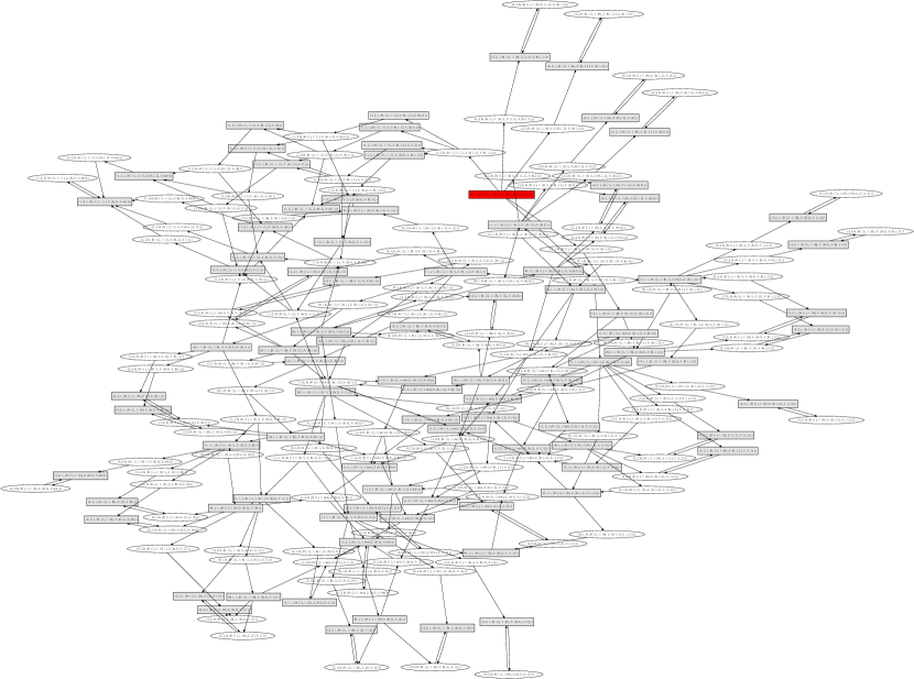
Figure 8: The game arena of Experiment 1.

Figure 9 is the hypergame transition system given P1’s sure winning strategy and P2’s perceived winning strategy in experiment 1.

Figure 9: The winning regions of two players in Experiment 1.

References

- [1] Rachid Ait Maalem Lahcen, Ram Mohapatra, and Manish Kumar. Cybersecurity: A survey of vulnerability analysis and attack graphs, volume 253. Springer Singapore, 2018.
- [2] Ehab Al-Shaer, Jinpeng Wei, Kevin W. Hamlen, and Cliff Wang. Dynamic Bayesian Games for Adversarial and Defensive Cyber Deception. In Ehab Al-Shaer, Jinpeng Wei, Kevin W. Hamlen, and Cliff Wang, editors, Autonomous Cyber Deception: Reasoning, Adaptive Planning, and Evaluation of HoneyThings, pages 75–97. Springer International Publishing, Cham, 2019.
- [3] Peter G Bennett. Hypergames: developing a model of conflict. Futures, 12(6):489–507, 1980.
- [4] J Richard Büchi and Lawrence H Landweber. Solving sequential conditions by finite-state strategies. Transactions of the American Mathematical Society, 138:295–311, 1969.
- [5] Thomas E. Carroll and Daniel Grosu. A Game Theoretic Investigation of Deception in Network Security. In 2009 Proceedings of 18th International Conference on Computer Communications and Networks, pages 1–6, August 2009.
- [6] Tanmoy Chakraborty, Sushil Jajodia, Noseong Park, Andrea Pugliese, Edoardo Serra, and VS Subrahmanian. Hybrid adversarial defense: Merging honeypots and traditional security methods. Journal of Computer Security, 26(5):615–645, 2018.
- [7] Edmund Clarke, Orna Grumberg, Somesh Jha, Yuan Lu, and Helmut Veith. Counterexample-guided abstraction refinement. In International Conference on Computer Aided Verification, pages 154–169. Springer, 2000.
- [8] Fred Cohen. The Use of Deception Techniques: Honeypots and Decoys. In Handbook of Information Security 3.1. 2006.
- [9] Javier Esparza, Jan Křetínskỳ, and Salomon Sickert. From LTL to deterministic automata. Formal Methods in System Design, 49(3):219–271, 2016.
- [10] Emmanuel Filiot, Naiyong Jin, and Jean François Raskin. Antichains and compositional algorithms for LTL synthesis. Formal Methods in System Design, 39(3):261–296, 2011.
- [11] Karel Horák, Branislav Bošanský, Christopher Kiekintveld, and Charles Kamhoua. Compact Representation of Value Function in Partially Observable Stochastic Games. In Proceedings of the Twenty-Eighth International Joint Conference on Artificial Intelligence, pages 350–356. International Joint Conferences on Artificial Intelligence Organization, 2019.
- [12] Kyle Ingols, Richard Lippmann, and Keith Piwowarski. Practical attack graph generation for network defense. In The 22nd Annual Computer Security Applications Conference, pages 121–130. IEEE, 2006.
- [13] Sushil Jajodia, V. S. Subrahmanian, Vipin Swarup, and Cliff Wang. Cyber deception: Building the scientific foundation. Springer, 2016.
- [14] S. Jha, O. Sheyner, and J. Wing. Two formal analyses of attack graphs. Proceedings of the Computer Security Foundations Workshop, 2002-Jan:49–63, 2002.
- [15] Abhishek Ninad Kulkarni and Jie Fu. A Compositional Approach to Reactive Games under Temporal Logic Specifications. In American Control Conference, pages 2356–2362. IEEE, 2018.
- [16] Orna Kupferman and Moshe Y Vardi. Model checking of safety properties. Formal Methods in System Design, 19(3):291–314, 2001.
- [17] Jiaqiang Liu, Yong Li, Huandong Wang, Depeng Jin, Li Su, Lieguang Zeng, and Thanos Vasilakos. Leveraging software-defined networking for security policy enforcement. Information Sciences, 327:288–299, 2016.
- [18] Zohar Manna and Amir Pnueli. The temporal logic of reactive and concurrent systems: Specification. Springer Science & Business Media, 2012.
- [19] Peng Ning, Yun Cui, Douglas S Reeves, and Dingbang Xu. Techniques and tools for analyzing intrusion alerts. ACM Transactions on Information and System Security, 7(2):274–318, 2004.
- [20] Steven Noel. Managing Attack Graph Complexity through Visual Hierarchical Aggregation. In In VizSEC/DMSEC ’04: Proceedings of the 2004 ACM Workshop on Visualization And, pages 109–118. ACM Press, 2004.
- [21] Jeffrey Pawlick, Edward Colbert, and Quanyan Zhu. A Game-theoretic Taxonomy and Survey of Defensive Deception for Cybersecurity and Privacy. ACM Comput. Surv., 52(4):82:1–82:28, August 2019.
- [22] A. Pnueli and R. Rosner. On the synthesis of a reactive module. In Proceedings of the 16th ACM SIGPLAN-SIGACT Symposium on Principles of Programming Languages, POPL ’89, pages 179–190, New York, NY, USA, 1989. ACM.
- [23] Alex Ramos, Marcella Lazar, Raimir Holanda Filho, and Joel J.P.C. Rodrigues. Model-Based Quantitative Network Security Metrics: A Survey. IEEE Communications Surveys and Tutorials, 19(4):2704–2734, 2017.
- [24] Tuomas W. Sandholm. Distributed rational decision making, 1999.
- [25] O. Sheyner, J. Haines, S. Jha, R. Lippmann, and J.M. Wing. Automated generation and analysis of attack graphs. In Proceedings 2002 IEEE Symposium on Security and Privacy, pages 273–284. IEEE Computer Society, 2002.
- [26] Oleg Mikhail Sheyner. Scenario graphs and attack graphs. PhD thesis, Carnegie Mellon University, 2004.
- [27] AJ Underbrink. Effective cyber deception. In Cyber Deception, pages 115–147. Springer, 2016.
- [28] Russell Richardson III Vane. Using Hypergames to Select Plans in Competitive Environments. PhD thesis, George Mason University, 2000.