DeepLight: Deep Lightweight Feature Interactions for Accelerating CTR Predictions in Ad Serving

Abstract.

Click-through rate (CTR) prediction is a crucial task in recommender system and online advertising. The embedding-based neural networks have been proposed to learn both explicit feature interactions through a shallow component and deep feature interactions by a deep neural network (DNN) component. These sophisticated models, however, slow down the prediction inference by at least hundreds of times. To address the issue of significantly increased serving latency and high memory usage for real-time serving in production, this paper presents DeepLight: a framework to accelerate the CTR predictions in three aspects: 1) accelerate the model inference via explicitly searching informative feature interactions in the shallow component; 2) prune redundant parameters at the inter-layer level in the DNN component; 3) prune the dense embedding vectors to make them sparse in the embedding matrix. By combining the above efforts, the proposed approach accelerates the model inference by 46X on Criteo dataset and 27X on Avazu dataset without any loss on the prediction accuracy. This paves the way for successfully deploying complicated embedding-based neural networks in real-world serving systems.

1. Introduction

Online advertising has grown into a hundred-billion-dollar business since 2020, and the revenue has been increasing by more than 15% per year for nine consecutive years (Bureau, 2020). CTR prediction is critical in the online advertising industry, and the main goal is to deliver the right ads to the right users in the right context. Therefore, how to predict CTR accurately and efficiently has drawn the attention of both academic and industry communities.

Generalized linear models and factorization machine (FM) (Rendle, 2010) have achieved great successes. However, they are limited in their prediction power due to the lack of mechanisms to learn deeper feature interactions. To tackle this issue, the embedding-based neural networks seek inspirations from computer vision and natural language processing and propose to include a shallow component to learn the informative low-order feature interactions and a DNN component for powerful high-order interaction modeling. In particular, Wide & Deep (Cheng et al., 2016) proposed to train a joint network that combines a linear model and a DNN model, which, however, still requires feature engineering and is not end-to-end. DeepFM (Guo et al., 2017) solved that problem by learning low-order feature interactions through the FM component instead of the linear model. Since then, various embedding-based neural networks have been proposed to improve the performance: Neural Factorization Machines (NFM) (He and Chua, 2017) uses a bilinear interaction pooling to connect the embedding vectors with the DNN component; Deep & Cross Network (DCN) (Wang et al., 2017) models cross features of bounded degrees in terms of layer depth; eXtreme Deep Factorization Machine (xDeepFM) (Lian et al., 2018) incorporates a Compressed Interaction Network (CIN) (Wang et al., 2017) and a DNN to automatically learn high-order feature interactions in both explicit and implicit manners; AutoInt (Song et al., 2019) proposes to model high-order feature interactions using self-attentive neural networks with residual connections; AutoFIS (Liu et al., 2020) proposes to identify important high-order feature interactions in the factorization machines for a more effective representation. Other extensions of embedding-based neural networks include (Qu et al., 2016; Shan et al., 2016; Chen et al., 2020; Zhou et al., 2014).

Despite the advances of these novel models applied in click prediction tasks in online advertising, the prediction is slowed down by hundreds of times compared to simple models such as logistic regression or factorization machine. This leads to unrealistic latency for the real-time ad serving system. One question that naturally follows is: are we able to serve the high quality deep models with satisfactory model latency and resource consumption for real-time response in ad serving?

Towards this goal, a practical solution needs to address the following challenges (C1-C3).

(C1) High quality: the served “slim” model is expected to be as accurate as the the original “fat” model.

(C2) Low latency: the serving latency should be at very low level to maintain high QPS (Query per second) with few timeout.

(C3) Low consumption: memory costs should be low for pulling model checkpoint and storing them in memory in online ad serving.

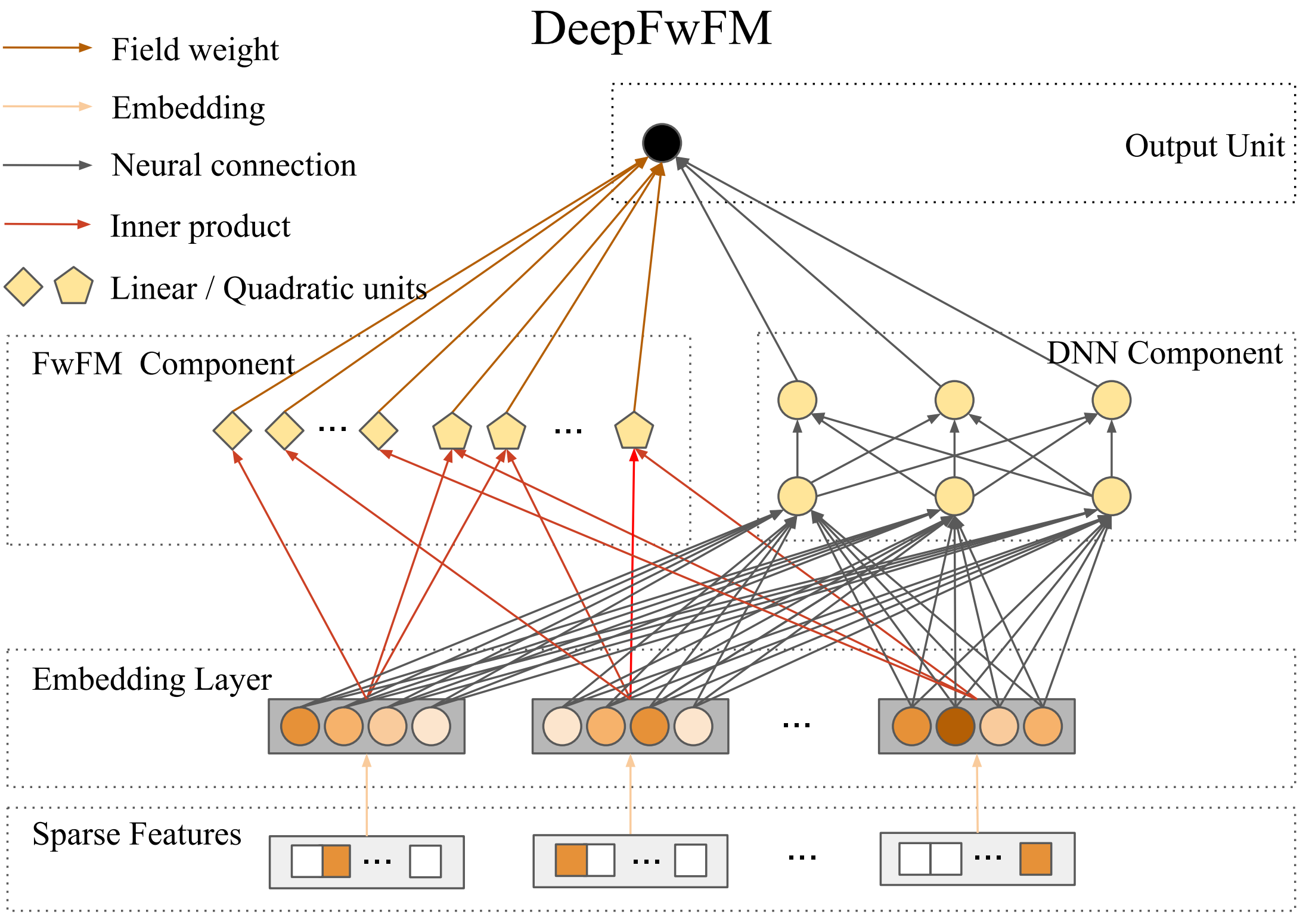
However, all the existing embedding-based neural networks, such as DeepFM, NFM, xDeepFM, and AutoInt, still focus on increasing the model complexity to achieve (C1) while sacrificing the performance in (C2) and (C3). Whereas a few approaches, such as AutoCross (Luo et al., 2019), are proposed to improve the model efficiency, they didn’t adopt the DNN framework and fail in achieving the state-of-the-art. To address these challenges all together, we propose an efficient model, so-called field-weighted embedding-based neural network (DeepFwFM) by improving the FM module via a field pair importance matrix, which is empirically as powerful as xDeepFM but becomes much more efficient. As shown in Figure 2, each component of DeepFwFM has an approximately sparse structure, which implies an advantage in structural pruning and potentially leads to an even more compact structure. By pruning the DNN component of DeepFwFM and further compressing the shallow component, the resulting deep lightweight structure, DeepLight, greatly reduces the inference time and still maintains the model performance. By contrast, the other structures may fail in either deep model accelerations (He and Chua, 2017; Wang et al., 2017; Lian et al., 2018; Liu et al., 2020) or accurate predictions (Guo et al., 2017; Cheng et al., 2016; Song et al., 2019).

To the best of our knowledge, this is the first paper that studies pruning embedding based DNN models for accelerating CTR predictions in ad serving. To summarize, the proposed field-weighted embedding-based neural network (DeepFwFM) has a great potential in fast and accurate inference. Compared to the existing embedding-based neural networks, the model has the following advantages:

$\bullet$ To address the challenge of (C1) high quality, the proposed model exploits the field pair importance idea in FwFM (Pan et al., 2018, 2019) to improve the understanding of low-order feature interactions instead of exploring high-order feature interactions (Wang et al., 2017; Lian et al., 2018). Most notably, such an improvement achieves the state-of-the-art with a very low complexity compared to the state-of-the-art xDeepFM model and still shows a great potential in deep model accelerations.

$\bullet$ To address the challenge of (C2) low latency, the model can be pruned for further acceleration: 1) prune redundant parameters in the deep component to obtain the most accelerations; 2) remove the weak field pairs in FwFM to obtain additional significant accelerations. The resulting lightweight structure ends up with almost a hundred times of accelerations.

$\bullet$ To address the challenge of (C3) low consumption, we can promote sparsity on the embedding vectors and preserve the most discriminant signals, which yields a substantial compression w.r.t. number of parameters.

By overcoming these challenges (C1-C3), the resulting sparse DeepFwFM, so-called DeepLight, eventually achieves remarkable performance not only in predictions, but also in deep model accelerations. It achieves 46X speed-ups on Criteo dataset and 27X speed-ups on Avazu dataset without loss on AUC. To help reproduce the results and benefit the community, we have made code available at https://github.com/WayneDW/sDeepFwFM.

2. Related Work

CTR prediction is typically achieved by feeding a machine learning model with well-designed features (He et al., 2014; McMahan et al., 2013). There have been extensive efforts on building features, such as textual features (Shaparenko et al., 2009), click feedback features (Graepel et al., 2010), contextual features (McMahan et al., 2013), and psychology features (Wang et al., 2013). To avoid the costly feature engineering, we need to build an end-to-end model by modeling feature interactions automatically. Given a dataset $\mathcal{D}=\{(y_{i},\bm{x}_{i})\}$, where $y_{i}$ is the label and $\bm{x}_{i}$ is a $m$-dimensional sparse feature vector, we can consider a degree-2 polynomial $\phi_{\text{Poly2}}$

(1) $$\min_{\bm{w}}\frac{\lambda}{2}\|\bm{w}\|_{2}^{2}+\sum_{i=1}^{|\mathcal{D}|}\log(1+\exp(-y_{i}\phi_{\text{Poly2}}(\bm{w},\bm{x_{i}}))),$$

where $\bm{w}$ is the model parameter, $\lambda$ is the $L_{2}$ penalty, $|\mathcal{D}|$ is the number of data points, and

(2) $$\phi_{\text{Poly2}}(\bm{w},\bm{W})=w_{0}+\sum_{i=1}^{m}x_{i}w_{i}+\sum_{i=1}^{m}\sum_{j=i+1}^{m}x_{i}x_{j}W_{i,j}.$$

Estimating the feature interaction matrix $\bm{W}$ in (2) given insufficient data is not easy, FM (Rendle, 2010) proposed a matrix decomposition method to learn the $k$-dimensional embedding vectors $\{\bm{e_{i}}\}_{i=1}^{m}$ through the inner product $\langle\bm{e}_{i},\bm{e}_{j}\rangle$:

(3) $$\phi_{\text{FM}}(\bm{w},\bm{e})=w_{0}+\sum_{i=1}^{m}x_{i}w_{i}+\sum_{i=1}^{m}\sum_{j=i+1}^{m}x_{i}x_{j}\langle\bm{e}_{i},\bm{e}_{j}\rangle.$$

Notably, the embedding vectors $\{\bm{e}_{i}\}_{i=1}^{m}$ reduces the number of parameters from $O(m^{2})$ to $O(mk)$. Although the above idea can be naturally extended to higher-order FMs, there is no efficient algorithm for training these models (Blondel et al., 2016). As such, Deep & Cross (Wang et al., 2017) tackles that problem by a series of cross operations:

(4) $$\bm{s}_{l}=\bm{s}_{0}\bm{s}^{T}_{l-1}w_{l}+\bm{b}_{l}+\bm{s}_{l-1},$$

where $\bm{w}_{l},\bm{b}_{l},\bm{s}_{l}$ denote the weights, bias and output of the $l$-th layer of the DeepCross network, respectively. Such an improvement alleviates the computation problems in solving high-order FM models and becomes quite powerful in modeling low-order feature interactions. By further combining a DNN component, we can obtain xDeepFM(Lian et al., 2018), which is the state-of-the-art model in CTR predictions.

(a) DeepFM

(b) DeepFwFM (the proposed unpruned model)

Figure 1. A model architecture comparison between DeepFM and proposed DeepFwFM. The inner products in the linear part of DeepFwFM are simplified. DNN component is generally built via the standard fully connected layers.

3. DeepFwFM: An Efficient Model

Considering the increasing latency concern of deploying complicated embedding-based neural networks in the real-world serving system, our goal is not only to build a model as accurate as xDeepFM (Lian et al., 2018) but also to show the potential for significant deep model accelerations. Despite the powerful performance in modeling feature interactions, xDeepFM (Lian et al., 2018) is known to be much more costly than DeepFM (Lian et al., 2018; Luo et al., 2019) and raises the risks in deep model accelerations. Such a problem motivates us to step back and rethink the framework of DeepFM. However, it is known that an ill-conditioned matrix suffers from a serious stability issue in matrix decomposition (Mackey et al., 2015; Li et al., 2016) and affects the performance of DeepFM.

3.1. Model architecture

To solve the stability issue, we seek inspirations from the preconditioner for robust matrix decompositions and consider the FwFM model (Pan et al., 2018), which includes the field pair importance to further improve the training of FM. In what follows, we propose the Deep Field-weighted Factorization Machine (DeepFwFM) by replacing $\phi_{\text{Poly2}}$ in (1) with $\phi_{\text{DeepFwFM}}$:

(5) $$\begin{split}&\phi_{\text{DeepFwFM}}(\bm{w},\bm{v},\bm{e},\mathbf{R})=\phi_{\text{Deep}}(\bm{w},\bm{e})+\phi_{\text{FwFM}}(\bm{v},\bm{e},\mathbf{R}),\\ \end{split}$$

where $\bm{w}$ is the DNN parameter that contains the weights and bias, $\bm{v}\in\mathbb{R}^{n\times k}$, $\bm{e}$ denotes the set of embedding vectors, $\mathbf{R}\in\mathbb{R}^{n\times n}$ is a matrix to model field pair interaction strength, and $\phi_{\text{FwFM}}$ is an efficient model(Pan et al., 2018) in studying second-order feature interactions on multi-field categorical data such that

(6) $$\small{\phi_{\text{FwFM}}(\bm{v},\bm{e},\mathbf{R})=w_{0}+\sum_{i=1}^{m}x_{i}\langle\bm{e}_{i},\bm{v}_{F(i)}\rangle+\sum_{i=1}^{m}\sum_{j=i+1}^{m}x_{i}x_{j}\langle\bm{e}_{i},\bm{e}_{j}\rangle R_{F(i),F(j)},}$$

where $F(i)$ denotes the field of feature $i$, $\bm{v}_{F(i)}$ denotes the linear embedding vector for field $F(i)$, $R_{F(i),F(j)}$ denotes the field pair interaction weight between field pair $(F(i),F(j))$ and $\phi_{\text{Deep}}$ is a non-linear transformation of the embeddings through a Multilayer Perceptron to learn high-order feature interactions.

To summarize, our model has the following innovations:

1) DeepFwFM is much faster than xDeepFM in that we don’t attempt to model high-order (3rd or more) feature interactions via the shallow component. Whereas xDeepFM contains a powerful compressed interaction network (CIN) to approximate any fixed-order of polynomials, the major drawback is that CIN has an even higher time complexity than the DNN component as discussed in (Lian et al., 2018), resulting in expensive computations in large-scale ad systems;

2) DeepFwFM is more accurate than DeepFM because it overcomes the stability issue in matrix decomposition and leads to more accurate predictions (Juan et al., 2016; Pan et al., 2018) by considering the field pair importance. DeepFM models low-order feature interactions through the weight-1 connections between each hidden node in the FM component and the output node as shown in Fig. 1, which, however, fails to adapt to the local geometry and sacrifices the robustness.

(a) Criteo: DNN component

(b) Criteo: Field matrix $R$

(c) Criteo: Embedding vectors

(d) Avazu: DNN component

(e) Avazu: Field matrix $R$

(f) Avazu: Embedding vectors

Figure 2. Weight demonstration of DeepFwFM model on Criteo and Avazu datasets. In particular for the DNN component and embedding vectors, we only choose a representative part to present due to their complexity. Moreover, we apply the magnitude-based max pooling operation to large matrices for illustration purposes.

3.2. Benefits of computation efficiency

To demonstrate the benefits of our model, we perform quantitative analysis for computational complexity of DeepFwFM, compared to DeepFM and xDeepFM.

Computational complexity

Given the embedding size $k$, the number of layers $l$, and the number of nodes in each layer $h$, the embedding layer only has $n$ lookups and leads to little computational cost. The number of floating point operations (FLOPs) of the DNN component and the FwFM component is $\mathcal{O}(lh^{2}+nkh)$ and $\mathcal{O}(n^{2}k)$, respectively. Similarly, we can derive the computational complexity of DeepFM (Guo et al., 2017) and xDeepFM (Lian et al., 2018). We summarize the results in Table.1 and observe that a $l$-layer CIN in xDeepFM takes $\mathcal{O}(nkh_{c}^{2}l)$ operations (Lian et al., 2018), which is much more than the DNN component. By contrast, the FM component and FwFM component is much faster than the DNN component. For example, considering standard parameter settings in Table.1, we see that theoretically DeepFwFM is as efficient as DeepFM and is 18X faster than xDeepFM.

Despite the initial progresses on accelerating CTR predictions, DeepFwFM still fails to reduce the latency to a good level (e.g. 10 ms for each bid request). In fact, DeepFwFM can be hundreds-of-times slower due to the inclusion of the DNN component, which significantly slows down the online CTR predictions.

Table 1. Computational complexity for three standard deep models. For example, a popular choice in Criteo dataset is to set $l=3$, $h=400$, $n=39$, $k=10$, $h_{c}=100$. As a result, the computations for DeepFM, xDeepFM and DeepFwFM are of order 0.64M, 12M and 0.65M, respectively.

Data	shallow component	DNN component
DeepFM	$\mathcal{O}(nk)$	$\mathcal{O}(lh^{2}+nkh)$
xDeepFM	$\mathcal{O}(nkh_{c}^{2}l)$	$\mathcal{O}(lh^{2}+nkh)$
DeepFwM	$\mathcal{O}(n^{2}k)$	$\mathcal{O}(lh^{2}+nkh)$

4. DeepLight: A Lightweight model via Structural pruning

The DNN component is undoubtedly the main reason that causes the high latency issue and fails to meet the online requirement. Therefore, a proper acceleration method is on great demand to speed up the predictions.

4.1. Why structural pruning?

Deep model acceleration has achieved great popularity in computer vision and it consists of three main methods: structural pruning (Han et al., 2015; Li et al., 2017), knowledge distillation (Hinton et al., 2015), and quantization (Courbariaux and Bengio, 2016), among which structural pruning methods have received wide attentions (Han et al., 2015, 2016; Deng et al., 2019; Wen et al., 2016; Li et al., 2018; Ye et al., 2020a; Ye et al., 2020b) due to their remarkable performance. Moreover, each component of DeepFwFM, such as the DNN component, the field pair interaction matrix $R$ and the embedding vectors, possesses the highly-sparse structure as shown in Figure.2. This motivates us to consider structural pruning to accelerate both the shallow component and the DNN component.

For the other choices, quantization  (Han et al., 2016) adopts the effective fixed point precision in inference time. However, it doesn’t fully utilize the sparse structure of each component of DeepFwFM and even damages the precision of large coefficients. While knowledge distillation technique (Hinton et al., 2015) trains small networks (i.e. student model) to mimic larger ones (i.e., teacher model), it suffers from the following issues: a) the student model may have a limited capacity to learn from the teacher; b) where there is a performance deterioration issue, it’s hard to figure out whether it’s due to the teacher model or due to the teaching procedure.

That’s the reason why we adopt structure pruning for CTR prediciton models in this work.

4.2. How to do structural pruning?

Design In this section, we show how to do structural pruning for DeepFwFM. Instead of simply applying pruning technique in ad prediction task with a uniform sparse rate, we propose to prune the following three components (in the context of DeepFwFM model) that are particularly designed to adapt for ad prediction task (given the existing feature embedding and field relevance in shallow and deep components):

$\bullet$ Prune the weights (excluding bias) of the DNN component to remove the neural connections;

$\bullet$ Prune the field pair interaction matrix $\bm{R}$ to remove redundant field interactions;

$\bullet$ Prune the elements in the embedding vectors, leading to sparse embedding vectors.

Combining the above efforts, we obtain the desired DeepLight model, as shown in Fig. 3. DeepLight is a sparse DeepFwFM that provides a holistic approach to accelerate inference by modifying the trained architecture at inference time.

Figure 3. DeepLight: A sparse architecture of DeepFwFM. The inner products in the linear part are simplified.

Benefit As is evident in empirical study, DeepLight enjoys the following properties

$\bullet$ The sparse DNN component has much less computation complexity, compared with the original one. It leads to the most accelerations in computation;

$\bullet$ The sparse field pair interaction matrix $\bm{R}$ further achieves significant accelerations in the FwFM component. In addition, pruning $\bm{R}$ is actually doing feature selection, or more accurately, field pair selection. Once a field pair interaction weight $R_{F,F^{\prime}}$ is pruned, all feature pairs from field pair $(F,F^{\prime})$ are dropped. AutoFIS (Liu et al., 2020) also achieves a similar kind of field pair selection;

$\bullet$ The sparse embedding greatly reduces the memory usage, since the feature embeddings dominate the number of parameters in deep learning models for click prediction.

Implementation Selecting a good sparse network from an over-parameterized model is NP-hard, and no optimal algorithms are guaranteed to solve it. There are a lot of empirical studies existed in the area of structural pruning (Han et al., 2015, 2016; Frankle and Carbin, 2019; Deng et al., 2019), including weight pruning, neuron pruning, or pruning of other units. Considering the fact that our model only contains a standard FwFM component and a vanilla DNN component, we conduct weight pruning and seek to achieve high sparsity and accelerations without calling specifically dedicated libraries.

Regarding the implementations, we adopt a standard algorithm used in (Deng et al., 2019; Frankle and Carbin, 2019) to study the structural pruning of the mainstream CTR-prediction models and compare them with our proposed sparse DeepFwFM, namely DeepLight. As in most of the pruning works, we put the community wisdom in our algorithm by adopting the $L_{2}$ penalty (Han et al., 2015, 2016). Now, we present the main algorithm in Alg.1. We first train the model a few epochs to provide a good initialization and then conduct pruning to remove the redundant weights with the lowest magnitude. After each pruning, we retrain the model to fine-tune the network so that mistakenly pruned weights has a potential to become active again. We keep repeating this pruning procedure and set adaptive sparse rates such that the rate increases faster in the early phase when the network is stable and slower in the late phase when the network becomes sensitive. The algorithm behaves similar to the greedy algorithms based on the weak sub-modular optimization (Das and Kempe, 2011), but it also injects some additional uncertainty during the pruning process, which potentially avoids damaging good weights.

Algorithm 1 Structural pruning for a target model, the target sparse rate $S\%=99\%$ means 99% of the parameters are pruned.

1:  Input Set the target sparse rate ${S}$, damping ratios $\mathbb{D}$ and $\mathbb{f}$.

2:  Warm up Initialize a neural network by training $i$ epochs.

3:  Pruning For $k=1,2,...$ do     Train the network for one iteration.     Enumerate the candidate component $X$ in a model         Update the current sparse rate $s_{X}\leftarrow{S_{X}}(1-\mathbb{D}^{k/{\mathbb{f}}})$.         Prune the bottom-$s_{X}\%$ lowest magnitude weights.

4:  Online Prediction Transform the sparse model to efficient structure.

4.3. Reduction of computational complexity

The DNN component is the bottleneck that causes the high inference time. After the pruning of the DNN component, the FwFM component becomes the limitations, which requires further pruning on the field matrix $\bm{R}$. The pruning of the embedding layer has no significant speed-ups on the computations.

With a medium $S_{\text{dnn}}\%$ sparsity on the weights in the DNN component (excluding the bias), the corresponding speed-ups can be close to the ideal $1/(1-S_{\text{dnn}}\%)$ times. However, when the sparsity $S_{\text{dnn}}\%$ is higher than 95%, we may not achieve the ideal rate because of the computations in the biases and the overhead of sparse structures, such as the compressed row storage (CRS). As to the pruning of the field matrix $\bm{R}$, the speed-ups becomes more significant as we increase the sparsity $S_{\text{dnn}}\%$ in the DNN component.

Table 2. Model comparison on the Criteo and Avazu datasets.

Criteo					Avazu
Models	Test		# Parameters	Latency ($ms$)	Test		# Parameters	Latency ($ms$)
	LogLoss	AUC			LogLoss	AUC
LR	0.4615	0.7881	1,326,056	0.001	0.3904	0.7617	1,544,393	0.001
FM	0.4565	0.7949	14,586,606	0.005	0.3816	0.7782	32,432,233	0.009
FwFM	0.4466	0.8049	13,261,682	0.145	0.3764	0.7866	30,888,853	0.105
DeepFM	0.4495	0.8036	15,064,206	4.181	0.3780	0.7852	32,751,433	2.719
NFM	0.4497	0.8030	15,204,206	4.091	0.3777	0.7854	32,689,033	2.704
xDeepFM	0.4420	0.8102	15,508,958	40.85	0.3749	0.7894	32,927,058	7.129
DeepFwFM	0.4403	0.8116	13,739,321	4.271	0.3751	0.7893	31,208,053	2.824

4.4. Reduction of space complexity

Pruning in the embedding layer also dramatically reduces the number of parameters in DeepFwFM and therefore saves lots of memory. In the embedding layer, a $S_{\text{emb}}\%$ sparsity reduces the number of parameters from $mk$ to $(1-S_{\text{emb}}\%)mk$. While in the DNN component, the number of weights (excluding the bias) can be reduced from $\mathcal{O}(nkh+lh^{2})$ to $\mathcal{O}\left((nhk+lh^{2})(1-S_{\text{dnn}}\%)\right)$ by storing the sparse weight matrix through the CRS. Similarly, a $S_{\text{R}}\%$ sparsity on the field matrix $\bm{R}$ reduces the parameters proportionally. Since the parameters in the embedding vectors dominate the total parameters in DeepFwFM, a $S_{\text{emb}}\%$ sparsity on the embedding vectors leads to the total memory reduction by roughly $1/(1-S_{\text{emb}}\%)$ times.

5. Experiments

5.1. Experimental setup

5.1.1. Data sets

1. Criteo Dataset: It is a well-known benchmark dataset for CTR prediction (Labs, 2014). It contains 45 million samples and each sample has 13 numerical features (counting) and 26 categorical features. We adopt the log transformation of $\log(x)^{2}$ if $x>2$ proposed by the winner of Criteo Competition to normalize the numerical features. We count the frequency of categorical features and treat all the features with a frequency less than 8 as unknown features. We randomly split the datasets into two parts: 90% is used for training and the rest is left for testing. 2. Avazu Dataset: We use the 10 days of click-through log on users’ mobile behaviors and randomly split 80% of the samples for training and leave the rest for testing. We treat the features with frequency less than 5 as unknown and replace them by a field-wise default feature. A description of the two datasets is shown in Table.3.

Table 3. Statistics of datasets

Data	Training set	# Fields	# Numerical	# Features
Criteo	41.3M	39	13	1.33M
Avazu	32.3M	23	0	1.54M

5.1.2. Evaluation metrics

To evaluate the prediction performance on Criteo dataset and Avazu dataset, we use LogLoss and AUC where LogLoss is the cross-entropy loss to evaluate the performance of a classification model and AUC is the area under the ROC curve to measure the probability that a random positive sample is ranked higher than a random negative sample.

5.1.3. Baselines

Among the popular embedding-based neural networks such as PNN (Qu et al., 2016), Deep & Wide (Cheng et al., 2016), Deep Crossing (Shan et al., 2016), Deep Cross (Wang et al., 2017), AutoInt (Song et al., 2019), DeepFM (Guo et al., 2017), NFM (He and Chua, 2017) and xDeepFM (Lian et al., 2018), we choose the last three because they have similar architectures to DeepFwFM and they are also the state-of-the-art models for CTR prediction . As a result, the 6 baseline models to evaluate DeepFwFM are LR (Logistic regression), FM (Rendle, 2010), FwFM (Pan et al., 2018), DeepFM (Guo et al., 2017), NFM (He and Chua, 2017), xDeepFM (Lian et al., 2018).

5.1.4. Implementation details

We train our model using PyTorch. To make a fair comparison on Criteo dataset, we follow the parameter settings in (Guo et al., 2017; Lian et al., 2018) and set the learning rate to $0.001$. The embedding size is set to 10. The default settings for the DNN components of DeepFM, NFM, and xDeepFM are: (1) the network architecture is $400\times 400\times 400$; (2) the dropout rate is 0.5. Specifically for xDeepFM, the cross layer in the CIN architecture is $100\times 100\times 50$. We fine-tuned the $L_{2}$ penalty and set it to 3e-7. We use the Adam optimizer (Kingma and Ba, 2015) for all of the experiments and the minibatch is chosen as 2048. Regarding Avazu dataset, we keep the same settings except that the embedding size is 20, the $L_{2}$ penalty is 6e-7, and the DNN network structure is $300\times 300\times 300$. Regarding the training time (not inference time) in practice, all the models don’t differ each other too much. FwFM and DeepFwFM are slightly faster than DeepFM and xDeepFM due to the innovations in the linear terms, owing to the innovations in the inner products of FwFM and DeepFwFM.

5.2. DeepFwFM v.s. other dense models

The evaluations of dense models without pruning show the maximum potential that the over-parameterized models perform. From Table 2, we observe that LR underperforms the other methods by at least 0.7% on Criteo dataset and 1.7% on Avazu dataset in terms of AUC, which shows that feature interactions are critical to improving the CTR prediction. Most of the embedding-based neural networks outperform the low-order methods such as LR and FM, implying the importance of modeling high-order feature interactions. However, the low-order FwFM still wins over NFM and DeepFM, showing the strength of field matrix $\bm{R}$ to learn second-order feature interactions to adapt to the local geometry.

NFM utilizes a black-box DNN to implicitly learn the low-order and high-order feature interactions, which may potentially over-fit the datasets due to the lack of mechanism to identify the low-order feature interactions explicitly. Among all the embedding-based neural network models, xDeepFM and DeepFwFM achieves the best result on Criteo dataset and Avazu dataset and outperform the other models by roughly 0.7% on Criteo dataset and 0.4% on Avazu dataset in terms of AUC. However, the inference time of xDeepFM is almost ten times longer than DeepFwFM on Criteo dataset, showing the inefficiency in real-time predictions for large-scale ad serving systems.

5.3. The sparse model: DeepLight

Following Alg. 1 with damping ratios $\mathcal{D}=0.99$ and $\Omega=100$, we first train the network by 2 epochs for warm-ups, and then run 8 epochs for the pruning experiments. We prune the network every 10 iterations to reduce the computational cost.

Table 4. DeepFwFMs with sparse DNN components/ embedding vectorss v.s. DeepFwFMs with smaller DNN components/ embedding vectors. The DeepFwFM model with X nodes in each DNN layer is referred to as N-X; The DeepFwFM model with embedding size X is referred to as E-X. The baselines are chosen to have a close number of parameters of the sparse network.

Criteo						Avazu
Sparse model	Test		Model	Test		Sparse Model	Test		Model	Test
	Logloss	AUC		Logloss	AUC		LogLoss	AUC		LogLoss	AUC
No Pruning	0.4403	0.8115	N-400	0.4403	0.8115	No Pruning	0.3751	0.7893	N-300	0.3751	0.7893
D-90% & R-0% & F-0%	0.4398	0.8120	N-87	0.4414	0.8104	D-90% & R-0% & F-0%	0.3747	0.7898	N-57	0.3757	0.7883
D-95% & R-0% & F-0%	0.4399	0.8120	N-51	0.4421	0.8098	D-95% & R-0% & F-0%	0.3747	0.7896	N-32	0.3762	0.7875
D-98% & R-0% & F-0%	0.4401	0.8117	N-25	0.4429	0.8089	D-99% & R-0% & F-0%	0.3748	0.7895	N-9	0.3769	0.7864
D-99% & R-0% & F-0%	0.4405	0.8113	N-15	0.4438	0.8078	D-99.5% & R-0% & F-0%	0.3749	0.7892	N-6	0.3771	0.7862
No Pruning	0.4403	0.8115	E-10	0.4403	0.8115	No Pruning	0.3751	0.7893	E-20	0.3751	0.7893
D-0% & R-0% & F-20%	0.4402	0.8116	E-8	0.4404	0.8115	D-0% & R-0% & F-20%	0.3750	0.7895	E-16	0.3752	0.7890
D-0% & R-0% & F-40%	0.4401	0.8118	E-6	0.4407	0.8113	D-0% & R-0% & F-40%	0.3751	0.7891	E-12	0.3750	0.7889
D-0% & R-0% & F-60%	0.4404	0.8116	E-4	0.4412	0.8106	D-0% & R-0% & F-60%	0.3762	0.7881	E-8	0.3765	0.7874
D-0% & R-0% & F-80%	0.4406	0.8114	E-2	0.4423	0.8094	D-0% & R-0% & F-80%	0.3773	0.7857	E-4	0.3770	0.7859

5.3.1. DNN pruning for accelerations

When we prune the DNN component, only the weights of the DNN component are pruned. The biases of DNN, the field matrix $\bm{R}$ and the parameters in the embedding layer is treated as usual. We try different pruning rates to study the prediction performance and deep model accelerations. To show the superiority of network pruning on a large network over training from a smaller one, we compare the networks with different sparse rates to the networks of smaller structures.

As shown in Table.4 (top), we see the DeepFwFMs with sparse DNN components outperforms the dense DeepFwFMs even when the sparse rate is as high as 95% on Criteo dataset. This phenomenon remains the same until we increase the sparsity to 99% on Criteo dataset. By contrast, the corresponding small networks with similar number of parameters such as N-25 and N-15 obtain much worse results than the original N-400, showing the power of pruning an over-parametrized network over training from a smaller one. On Avazu dataset, we obtain the same conclusions. The sparse model obtains the best prediction performance with 90% sparsity and only goes worse when the sparsity is larger than 99.5%.

(a) Criteo.

(b) Avazu.

Figure 4. DNN pruning for accelerations.

Regarding the deep model acceleration, we see from Fig.4 that a larger sparsity always brings a lower latency and when the sparsity is 98% on Criteo dataset and 99% on Avazu dataset, we realize the performance is still surprisingly better than the original dense network and we achieve as large as 16X speed-ups on both datasets.

5.3.2. Pruning of the field matrix $\bm{R}$ for accelerations

After applying a high sparsity on the DNN component, we already obtain significant speed-ups which is close to 20X. To further boost the accelerations, increasing the sparsity on the DNN component may risk in decreasing the performance and doesn’t yield obvious accelerations due to the overhead in matrix computations. Recall from Fig.2 that the field matrix $\bm{R}$ possesses an approximately sparse structure. This motivates us to further prune the field matrix $\bm{R}$ to obtain deep accelerations. Given a 99% sparsity for the DNN component on the Criteo dataset (98% sparsity on the Avazu dataset), we study the sparse model performance based on different sparse rates in the field matrix $\bm{R}$. From Fig.5, we observe that we can adopt up-to 95% sparsity on the field matrix $\bm{R}$ without sacrificing the performance. Additionally, the predictions can be further accelerated by two to three times. As a result, we can eventually obtain 46X and 27X speed-ups without sacrificing the performance.

(a) Criteo

(b) Avazu

Figure 5. Pruning of the field matrix $\bm{R}$ for accelerations.

5.3.3. Pruning of embedding vectors for memory savings

As to the pruning of embeddings, we find that setting a global threshold for the embeddings of all fields obtains a slightly better performance than setting individual thresholds for the embedding vector from each field. Therefore, we conduct the experiments based on a global threshold.

(a) Criteo

(b) Avazu

Figure 6. Pruning of embedding vectors for memory savings.

Table 5. Structural pruning of DeepFwFM on Criteo dataset. D-90% & R-90% & F-40% is short for the sparse DeepFwFM which has 90% sparse rate on the DNN component and the field matrix $\bm{R}$ and a 40% sparse rate on the embedding vectors.

Dataset	Goal	Structural Pruning	Test		# Parameters	Latency ($ms$)
			Logloss	AUC
Criteo	None	No Pruning	0.4403	0.8116	13,739,321	4.271
	High performance	D-90% & R-90% & F-40%	0.4395	0.8123	8,012,094	0.469
	Low memory	D-90% & R-90% & F-90%	0.4404	0.8114	1,376,431	0.472
	Low latency	D-99% & R-95% & F-40%	0.4405	0.8114	7,413,578	0.093
Avazu	None	No Pruning	0.3751	0.7893	31,208,053	2.824
	High performance	D-90% & R-90% & F-20%	0.3748	0.7897	24,808,262	0.422
	Low memory	D-90% & R-90% & F-60%	0.3753	0.7892	9,322,791	0.318
	Low latency	D-98% & R-90% & F-0%	0.3753	0.7894	30,859,675	0.104

As shown in Fig.6, Criteo can adopt a high sparse rate, such 80%, to remain the same performance on Criteo dataset; by contrast, the model is sensitive on Avazu dataset and starts to decrease the performance when a 60% sparsity is applied. From Table. 4 (bottom), we see most of the models outperforms the baseline models (referred to as E-X) with a smaller embedding size, which sheds light on the use of large embedding sizes and pruning techniques to over-parameterize the network to avoid over-fitting.

5.3.4. Structural pruning of DeepFwFM

From the above experiments, we see that the DNN component and the field matrix $\bm{R}$ accept a much higher sparse rate to remain the same prediction performance, which inspires us to apply different pruning rates on the hybrid components.

As shown in Table.5, for the performance-driven tasks, we can improve the state-of-the-art AUC from 0.8116 to 0.8223 on Criteo dataset via a sparse DeepFwFM where 90% of the parameters in both the DNN component and the field matrix $\bm{R}$ and 40% of the parameters in the embedding vectors are pruned, and such model is denoted by D-90% & R-90% & F-40%. On Avazu dataset, a sparse DeepFwFM with structure D-90% & R-90% & F-20% further improves the state-of-the-art AUC from 0.7893 to 0.7897. For the memory-driven tasks, the memory savings are up to 10X and 2.5X on Criteo dataset and Avazu dataset, respectively. For the latency-driven tasks, we achieve 46X speed-ups on Criteo dataset using a DeepLight with the structure D-99% & R-95% & F-40% and 27X speed-ups on Avazu dataset using the structure D-98% & R-90% & F-0% without loss of accuracy.

5.4. DeepLight v.s. other sparse models

For the other models, we also try the corresponding best structure for accelerating the predictions without sacrificing the performance. With respect to the CIN component in xDeepFM, we denote the 99% sparsity on the CIN component by C-99%. We report the results in Table.6 and observe that all the embedding based neural networks adopt high sparse rates to maintain the performance. Moreover, DeepLight is comparable to sparse DeepFM and sparse NFM in terms of prediction time but improves the AUC by at least 0.8% on Criteo dataset and 0.4% on Avazu dataset. DeepLight obtains a similar prediction performance as xDeepFM but is almost 10X faster. This shows the superiority of DeepLight over sparse DeepFM, sparse NFM, sparse xDeepFM in large-scale online ad serving systems for both fast and accurate predictions.

Table 6. Evaluation of sparse models on Criteo and Avazu datasets. For each individual model, we only report the most efficient structure that yields the best accelerations with almost no sacrifice on the prediction performance.

Criteo					Avazu
Models	Test		Structure	Latency ($ms$)	Test		Structure	Latency ($ms$)
	LogLoss	AUC			LogLoss	AUC
Sparse DeepFM	0.4496	0.8032	D-98% & F-40%	0.114	0.3782	0.7851	D-98% & F-20%	0.102
Sparse NFM	0.4494	0.8031	D-98% & F-40%	0.114	0.3778	0.7854	D-98% & F-20%	0.102
Sparse xDeepFM	0.4421	0.8102	D-99% & C-99% & F-40%	0.907	0.3750	0.7893	D-98% & C-98% & F-0%	0.927
DeepLight	0.4405	0.8114	D-99% & R-95% & F-40%	0.093	0.3753	0.7894	D-98% & R-90% & F-0%	0.104

6. Conclusions

In this paper, we propose the lightweight DeepLight model for efficient CTR predictions. A key advantage of this model is that the field matrix $\bm{R}$ not only provides a robust matrix decomposition to improve the performance with little costs, but also possesses a highly-sparse structure with acceleration potentials after pruning. To the best of our knowledge, this is the first work of network pruning applied to the area of CTR prediction in online advertising to solve the high-latency issues. We observe that network pruning is not only powerful to prune redundant parameters to alleviate over-fitting but also achieves significant acceleration on the inference time and shows a pronounced reduction on the memory usage with little impact on the prediction performance.

References

- (1)
- Blondel et al. (2016) Mathieu Blondel, Akinori Fujino, Naonori Ueda, and Masakazu Ishihata. 2016. Higher-Order Factorization Machines. In NIPS’16.
- Bureau (2020) Interactive Advertising Bureau. 2020. IAB internet advertising revenue report. In Iab Pwc. 1–32.
- Chen et al. (2020) Wenqiang Chen, Lizhang Zhan, Yuanlong Ci, and Chen Lin. 2020. FLEN: Leveraging Field for Scalable CTR Prediction. In KDD’20 DLP workshop.
- Cheng et al. (2016) Heng-Tze Cheng, Levent Koc, Jeremiah Harmsen, Tal Shaked, Tushar Chandra, Hrishi Aradhye, Glen Anderson, Greg Corrado, Wei Chai, Mustafa Ispir, Rohan Anil, Zakaria Haque, Lichan Hong, Vihan Jain, Xiaobing Liu, and Hemal Shah. 2016. Wide & Deep Learning for Recommender Systems. (2016). arXiv:1606.07792
- Courbariaux and Bengio (2016) Matthieu Courbariaux and Yoshua Bengio. 2016. BinaryNet: Training Deep Neural Networks with Weights and Activations Constrained to +1 or -1. CoRR.
- Das and Kempe (2011) Abhimanyu Das and David Kempe. 2011. Submodular meets Spectral: Greedy Algorithms for Subset Selection, Sparse Approximation and Dictionary Selection. In ICML’11.
- Deng et al. (2019) Wei Deng, Xiao Zhang, Faming Liang, and Guang Lin. 2019. An Adaptive Empirical Bayesian Method for Sparse Deep Learning. In NeurIPS’19.
- Frankle and Carbin (2019) Jonathan Frankle and Michael Carbin. 2019. The lottery ticket hypothesis: Finding sparse, trainable neural networks. ICLR’19.
- Graepel et al. (2010) Thore Graepel, Joaquin Quiñonero Candela, Thomas Borchert, and Ralf Herbrich. 2010. Web-scale Bayesian Click-through Rate Prediction for Sponsored Search Advertising in Microsoft’s Bing Search Engine. In ICML’10.
- Guo et al. (2017) Huifeng Guo, Ruiming Tang, Yunming Ye, Zhenguo Li, and Xiuqiang He. 2017. DeepFM: A Factorization-Machine based Neural Network for CTR Prediction. In IJCAI-17.
- Han et al. (2016) Song Han, Huizi Mao, and William J. Dally. 2016. Deep Compression: Compressing Deep Neural Networks with Pruning, Trained Quantization and Huffman Coding. In ICLR’16.
- Han et al. (2015) Song Han, Jeff Pool, John Tran, and William Dally. 2015. Learning both weights and connections for efficient neural network. In NIPS’15.
- He and Chua (2017) Xiangnan He and Tat-Seng Chua. 2017. Neural Factorization Machines for Sparse Predictive Analytics. In SIGIR’17.
- He et al. (2014) Xinran He, Junfeng Pan, Ou Jin, Tianbing Xu, Bo Liu, Tao Xu, Yanxin Shi, Antoine Atallah, Ralf Herbrich, Stuart Bowers, and Joaquin Quinonero Candela. 2014. Practical Lessons from Predicting Clicks on Ads at Facebook. In ADKDD’14.
- Hinton et al. (2015) Geoffrey Hinton, Oriol Vinyals, and Jeffrey Dean. 2015. Distilling the Knowledge in a Neural Network. In NIPS Deep Learning and RL Workshop.
- Juan et al. (2016) Yuchin Juan, Yong Zhuang, Wei-Sheng Chin, and Chih-Jen Lin. 2016. Field-aware Factorization Machines for CTR Prediction. In RecSys’16.
- Kingma and Ba (2015) Diederik P. Kingma and Jimmy Ba. 2015. Adam: A Method for Stochastic Optimization. In ICLR’15.
- Labs (2014) Criteo Labs. 2014. Display Advertising Challenge. In Kaggle.
- Li et al. (2016) Chunyuan Li, Changyou Chen, David Carlson, and Lawrence Carin. 2016. Preconditioned Stochastic Gradient Langevin Dynamics for Deep Neural Networks. In AAAI’16.
- Li et al. (2018) Dawei Li, Xiaolong Wang, and Deguang Kong. 2018. DeepRebirth: Accelerating Deep Neural Network Execution on Mobile Devices. In AAAI’18.
- Li et al. (2017) Hao Li, Asim Kadav, Igor Durdanovic, Hanan Samet, and Hans Peter Graf. 2017. Pruning Filters for Efficient ConvNets. In ICLR’17.
- Lian et al. (2018) Jianxun Lian, Xiaohuan Zhou, Fuzheng Zhang, Zhongxia Chen, Xing Xie, and Guangzhong Sun. 2018. xDeepFM: Combining Explicit and Implicit Feature Interactions for Recommender Systems. KDD’18.
- Liu et al. (2020) Bin Liu, Chenxu Zhu, Guilin Li, Weinan Zhang, Jincai Lai, Ruiming Tang, Xiuqiang He, Zhenguo Li, and Yong Yu. 2020. AutoFIS: Automatic Feature Interaction Selection in Factorization Models for Click-Through Rate Prediction. In KDD’20.
- Luo et al. (2019) Yuanfei Luo, Mengshuo Wang, Hao Zhou, Quanming Yao, Wei-Wei Tu, Yuqiang Chen, Qiang Yang, and Wenyuan Dai. 2019. AutoCross: Automatic Feature Crossing for Tabular Data in Real-World Applications. In KDD’19.
- Mackey et al. (2015) Lester Mackey, Ameet Talwalkar, and Michael I. Jordan. 2015. Distributed Matrix Completion and Robust Factorization. JMLR’15 16 (2015), 913–960.
- McMahan et al. (2013) H. Brendan McMahan, Gary Holt, D. Sculley, Michael Young, Dietmar Ebner, Julian Grady, Lan Nie, Todd Phillips, Eugene Davydov, Daniel Golovin, Sharat Chikkerur, Dan Liu, Martin Wattenberg, Arnar Mar Hrafnkelsson, Tom Boulos, and Jeremy Kubica. 2013. Ad Click Prediction: a View from the Trenches. In KDD’13.
- Pan et al. (2019) Junwei Pan, Yizhi Mao, Alfonso Lobos Ruiz, Yu Sun, and Aaron Flores. 2019. Predicting different types of conversions with multi-task learning in online advertising. In KDD’19.
- Pan et al. (2018) Junwei Pan, Jian Xu, Alfonso Lobos Ruiz, Wenliang Zhao, Shengjun Pan, Yu Sun, and Quan Lu. 2018. Field-weighted Factorization Machines for Click-Through Rate Prediction in Display Advertising. In WWW’18.
- Qu et al. (2016) Yanru Qu, Han Cai, Kan Ren, Weinan Zhang, Yong Yu, Ying Wen, and Jun Wang. 2016. Product-based Neural Networks for User Response Prediction. CoRR (2016).
- Rendle (2010) Steffen Rendle. 2010. Factorization Machines. In ICDM’10.
- Shan et al. (2016) Ying Shan, T. Ryan Hoens, Jian Jiao, Haijing Wang, Dong Yu, and JC Mao. 2016. Deep Crossing: Web-Scale Modeling Without Manually Crafted Combinatorial Features. In KDD’16.
- Shaparenko et al. (2009) Benyah Shaparenko, Ozgur Cetin, and Rukmini Iyer. 2009. Data-driven Text Features for Sponsored Search Click Prediction. In ADKDD’09.
- Song et al. (2019) Weiping Song, Chence Shi, Zhiping Xiao, Zhijian Duan, Yewen Xu, Ming Zhang, and Jian Tang. 2019. AutoInt: Automatic Feature Interaction Learning via Self-Attentive Neural Networks. CIKM’19.
- Wang et al. (2017) Ruoxi Wang, Bin Fu, Gang Fu, and Mingliang Wang. 2017. Deep & Cross Network for Ad Click Predictions. arXiv:1708.05123
- Wang et al. (2013) Taifeng Wang, Jiang Bian, Shusen Liu, Yuyu Zhang, and Tie-Yan Liu. 2013. Psychological Advertising: Exploring User Psychology for Click Prediction in Sponsored Search. KDD’13.
- Wen et al. (2016) Wei Wen, Chunpeng Wu, Yandan Wang, Yiran Chen, and Hai Li. 2016. Learning Structured Sparsity in Deep Neural Networks. In NIPS’16.
- Ye et al. (2020a) Mao Ye, Chengyue Gong, Lizhen Nie, Denny Zhou, Adam Klivans, and Qiang Liu. 2020a. Good Subnetworks Provably Exist: Pruning via Greedy Forward Selection. In ICML’20.
- Ye et al. (2020b) Mao Ye, Lemeng Wu, and Qiang Liu. 2020b. Greedy Optimization Provably Wins the Lottery: Logarithmic Number of Winning Tickets is Enough. In NeurIPS’20.
- Zhou et al. (2014) Guorui Zhou, Xiaoqiang Zhu, Chengru Song, Ying Fan, Han Zhu, Xiao Ma, Yanghui Yan, Junqi Jin, Han Li, and Kun Gai. 2014. Deep Interest Network for Click-Through Rate Prediction. In KDD’14.