Abstract

For the search for additional Higgs bosons in the Minimal Supersymmetric Standard Model (MSSM) as well as for future precision analyses in the Higgs sector a precise knowledge of their production properties is mandatory. We review the evaluation of the cross sections for the neutral Higgs boson production in association with a photon at future $e^{+}e^{-}$ colliders in the MSSM with complex parameters (cMSSM). The evaluation is based on a full one-loop calculation of the production mechanism $e^{+}e^{-}\to h_{i}\gamma$ $(i=1,2,3)$. The dependance of the lightest Higgs-boson production cross sections on the relevant cMSSM parameters is analyzed numerically. We find relatively small numerical depedances of the production cross sections on the underlying parameters.

1 Introduction

The most frequently studied models for electroweak symmetry breaking are the Higgs mechanism within the Standard Model (SM) and within the Minimal Supersymmetric Standard Model (MSSM) [1, 2, 3]. Contrary to the case of the SM, in the MSSM two Higgs doublets are required. This results in five physical Higgs bosons instead of the single Higgs boson in the SM. In lowest order these are the light and heavy ${\cal CP}$-even Higgs bosons, $h$ and $H$, the ${\cal CP}$-odd Higgs boson, $A$, and two charged Higgs bosons, $H^{\pm}$. Within the MSSM with complex parameters (cMSSM), taking higher-order corrections into account, the three neutral Higgs bosons mix and result in the states $h_{i}$ ($i=1,2,3$) [4, 5, 6, 7]. The Higgs sector of the cMSSM is described at the tree-level by two parameters: the mass of the charged Higgs boson, $M_{H^{\pm}}$, and the ratio of the two vacuum expectation values, $\tan\beta\equiv t_{\beta}=v_{2}/v_{1}$. Often the lightest Higgs boson, $h_{1}$ is identified [8] with the particle discovered at the LHC [9, 10] with a mass around $\sim 125\,\,\mathrm{GeV}$ [11].

If supersymmetry (SUSY) is realized in nature the additional Higgs bosons could be produced at a future $e^{+}e^{-}$ collider such as the ILC [12, 13] or CLIC [14, 13], or at lower center-of-mass energies at FCC-ee [15] or CEPC [16]. In the case of a discovery of additional Higgs bosons a subsequent precision measurement of their properties will be crucial to determine their nature and the underlying (SUSY) parameters. In order to yield a sufficient accuracy, one-loop corrections to the various Higgs-boson production and decay modes have to be considered. Full one-loop calculations in the cMSSM for various Higgs-boson decays to SM fermions, scalar fermions and charginos/neutralinos have been presented over the last years [17, 18, 19]. For the decay to SM fermions see also Refs. [20, 21, 22]. Decays to (lighter) Higgs bosons have been evaluated at the full one-loop level in the cMSSM in Ref. [17]; see also Refs. [23, 24]. Decays to SM gauge bosons (see also Ref. [25]) can be evaluated using the full SM one-loop result [26] combined with the appropriate effective couplings [27] (see, however, Ref. [28]). The full one-loop corrections in the cMSSM listed here together with resummed SUSY corrections have been implemented into the code FeynHiggs [29, 30, 31, 27, 32, 33].

Particularly relevant are higher-order corrections also for the Higgs-boson production at $e^{+}e^{-}$ colliders, where a very high accuracy in the Higgs property determination is anticipated [13]. Available at the full one-loop level within the cMSSM are [34, 35]

$$\sigma(e^{+}e^{-}\to h_{i}h_{j})\,,$$ (1)

$$\sigma(e^{+}e^{-}\to h_{i}Z)\,,$$ (2)

$$\sigma(e^{+}e^{-}\to h_{i}\gamma)\,,$$ (3)

$$\sigma(e^{+}e^{-}\to H^{+}H^{-})\,,$$ (4)

$$\sigma(e^{+}e^{-}\to H^{\pm}W^{\mp})\,.$$ (5)

The processes $e^{+}e^{-}\to h_{i}h_{i}$, $e^{+}e^{-}\to h_{i}\gamma$ and $e^{+}e^{-}\to H^{\pm}W^{\mp}$ are purely loop-induced. Here we will review the results for the process $e^{+}e^{-}\to h_{1}\gamma$. We will concentrate on examples for the numerical results. Details on the renormalization of the cMSSM, the evaluation of the loop diagrams, the cancellation of UV divergences, as well as a comparison with previous, less advanced calculations can be found in Ref. [34].

2 Contributing diagrams

Figure 1: Generic vertex, box, and counterterm diagrams for the (loop-induced) process $e^{+}e^{-}\to h_{i}\gamma$ ($i=1,2,3$). $F$ can be a SM fermion, chargino or neutralino; $S$ can be a sfermion or a Higgs/Goldstone boson; $V$ can be a $\gamma$, $Z$ or $W^{\pm}$. It should be noted that electron–Higgs couplings are neglected.

Sample diagrams for the process $e^{+}e^{-}\to h_{i}\gamma$ $(i=1,2,3$) are shown in Fig. 1. The internal particles in the generically depicted diagrams in Fig. 1 are labeled as follows: $F$ can be a SM fermion $f$, chargino $\tilde{\chi}_{c}^{\pm}$ or neutralino $\tilde{\chi}_{n}^{0}$; $S$ can be a sfermion ${\tilde{f}}_{s}$ or a Higgs (Goldstone) boson $h_{i},H^{\pm}$ ($G,G^{\pm}$); $U$ denotes the ghosts $u_{V}$; $V$ can be a photon $\gamma$ or a massive SM gauge boson, $Z$ or $W^{\pm}$.

The diagrams and corresponding amplitudes have been obtained with FeynArts (version 3.9) [40], using the MSSM model file (including counter terms) of Ref. [41]. The further evaluation has been performed with FormCalc (version 8.4) and LoopTools (version 2.12) [42]. We have neglected all electron–Higgs couplings and terms proportional to the electron mass ME (and the squared electron mass ME2), except when it appears in negative powers or in loop integrals. We have verified numerically that these contributions are indeed totally negligible. For internally appearing Higgs bosons no higher-order corrections to their masses or couplings are taken into account; these corrections would correspond to effects beyond one-loop order. For external Higgs bosons, as discussed in Ref. [27], the appropriate $\hat{Z}$ factors are applied and on-shell (OS) masses (including higher-order corrections) are used [27], obtained with FeynHiggs [29, 30, 31, 27, 32, 33].

3 Numerical Examples

Here we review examples for the numerical analysis of the lightest neutral Higgs boson production in association with a photon at the ILC, CLIC, FCC-ee or CEPC. The process $e^{+}e^{-}\to h_{1}\gamma$ is purely loop-induced (via vertex and box diagrams) and therefore $\propto|{\cal M}_{\text{1-loop}}|^{2}$, where ${\cal M}_{\text{1-loop}}$ denotes the one-loop matrix element of the process.

3.1 Parameter settings

Details on the SM parameters can be found in Ref. [34]. The SUSY parameters are chosen according to the scenarios $\mathcal{S}$1 and $\mathcal{S}$2, shown in Tab. 1, unless otherwise noted. These scenarios constitutes viable scenarios for the various cMSSM Higgs production modes. While the charged Higgs-boson mass in $\mathcal{S}$1 is somewhat low w.r.t. the most recent exclusion bounds, this does not affect strongly the numerical evaluation reviewed here in this scenario. The Higgs sector quantities (masses, mixings, $\hat{Z}$ factors, etc.) have been evaluated using FeynHiggs (version 2.11.0 for $\mathcal{S}$1 and version 2.13.0 for $\mathcal{S}$2).

Table 1: MSSM default parameters for the numerical investigation; all parameters (except of $t_{\beta}$) are in GeV (calculated masses are rounded to 1 MeV). The values for the trilinear sfermion Higgs couplings, $A_{t,b,\tau}$ are chosen such that charge- and/or color-breaking minima are avoided [43].

Scen.	$\sqrt{s}$	$t_{\beta}$	$\mu$	$M_{H^{\pm}}$	$M_{\tilde{Q},\tilde{U},\tilde{D}}$	$M_{\tilde{L},\tilde{E}}$	$|A_{t,b,\tau}|$	$M_{1}$	$M_{2}$	$M_{3}$
$\mathcal{S}$1	500	7	200	300	1000	500	$1500+\mu/t_{\beta}$	100	200	1500
$\mathcal{S}$2	250	10	350	1200	2000	300	2600,2000,2000	400	600	2000

Scen.	$m_{h_{1}}$	$m_{h_{2}}$	$m_{h_{3}}$	FeynHiggs version
$\mathcal{S}$1	123.404	288.762	290.588	2.11.0
$\mathcal{S}$2	125.013	1197.081	1197.106	2.13.0

The numerical results shown in the next subsections are of course dependent on the choice of the SUSY parameters. Nevertheless, they give an idea of the relevance parameter dependances.

3.2 The process $e^{+}e^{-}\to h_{1}\gamma$: general dependances

In Fig. 2 we show the results for the process $e^{+}e^{-}\to h_{1}\gamma$ in $\mathcal{S}$1 as a function of $\sqrt{s}$, $M_{H^{\pm}}$, $t_{\beta}$ and $\varphi_{A_{t}}$. Not shown here are the processes $e^{+}e^{-}\to h_{i}\gamma$ ($i=2,3$) because they are at the border of observability, and the corresponding Higgs-boson masses are excluded by the most recent searches (see, however, Ref. [34]).

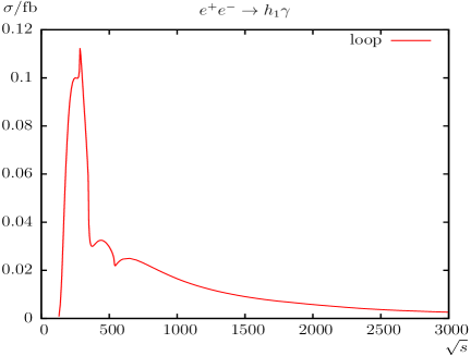
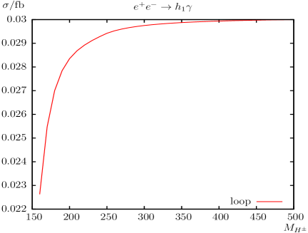
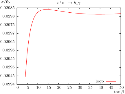
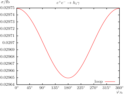
Figure 2: $\sigma(e^{+}e^{-}\to h_{1}\gamma)$. Loop induced (i.e. leading two-loop corrected) cross sections are shown with parameters chosen according to $\mathcal{S}$1 (see Tab. 1). The upper plots show the cross sections with $\sqrt{s}$ (left) and $M_{H^{\pm}}$ (right) varied; the lower plots show $t_{\beta}$ (left) and $\varphi_{A_{t}}$ (right) varied.

The largest contributions to $e^{+}e^{-}\to h_{1}\gamma$ are expected from loops involving top quarks and SM gauge bosons. The cross section is rather small for the parameter set chosen; see Tab. 1. As a function of $\sqrt{s}$ (upper left plot) a maximum of $\sim 0.1$ fb is reached around $\sqrt{s}\sim 250\,\,\mathrm{GeV}$, where several thresholds and dip effects overlap (see also Ref. [39] for a more general discussion). The first peak is found at $\sqrt{s}\approx 283\,\,\mathrm{GeV}$, due to the threshold $m_{\tilde{\chi}_{1}^{\pm}}+m_{\tilde{\chi}_{1}^{\pm}}=\sqrt{s}$. A dip can be found at $m_{t}+m_{t}=\sqrt{s}\approx 346\,\,\mathrm{GeV}$. The next dip at $\sqrt{s}\approx 540\,\,\mathrm{GeV}$ is the threshold $m_{\tilde{\chi}_{2}^{\pm}}+m_{\tilde{\chi}_{2}^{\pm}}=\sqrt{s}$. The loop corrections for $\sqrt{s}$ vary between $0.1$ fb at $\sqrt{s}\approx 250\,\,\mathrm{GeV}$, $0.03$ fb at $\sqrt{s}\approx 500\,\,\mathrm{GeV}$ and $0.003$ fb at $\sqrt{s}\approx 3000\,\,\mathrm{GeV}$. Consequently, this process could be observable for larger ranges of $\sqrt{s}$. In particular in the phase with $\sqrt{s}=500\,\,\mathrm{GeV}$ [45] 30 events could be produced with an integrated luminosity of ${\cal L}=1\,\mbox{ab}^{-1}$. As a function of $M_{H^{\pm}}$ (upper right plot) we find an increase in $\mathcal{S}$1, increasing the production cross sections from $0.023$ fb at $M_{H^{\pm}}\approx 160\,\,\mathrm{GeV}$ to about $0.03$ fb in the decoupling regime. This dependance shows the relevance of the SM gauge boson loops in the production cross section, indicating that the top quark loops dominate this production cross section. The variation with $t_{\beta}$ and $\varphi_{A_{t}}$ (lower row) is rather small, and values of $0.03$ fb are found in $\mathcal{S}$1.

3.3 The process $e^{+}e^{-}\to h\gamma$: beam polarization

Potentially larger cross sections can be realized with beam polarization. To analyze this, in Fig. 3 we show the results for the process $e^{+}e^{-}\to h\gamma$ (no complex parameters) in $\mathcal{S}$2 as a function of $\sqrt{s}$, see Ref. [44] for more details. The thick solid (gray) line indicates the cross section without beam polarization. The results with 100% polarizations of the positron and electron beam are shown as dotted, dash-dotted, dashed and solid (thin) lines for the combinations $(P_{e^{+}},P_{e^{-}})=(-,-),(-,+),(+,-),(+,+)$, respectively. One can see that $(+,-)$ ($(-,+)$) yield a larger (smaller) cross section as the unpolarized case. The polarizations $(-,-)$ and $(+,+)$ result in zero cross section. A realistic ILC value is given by $(P_{e^{+}},P_{e^{-}})=(+0.3,-0.8)$, which is shown as red solid line. This polarized cross section is larger than the unpolarized one by more than a factor of 2.

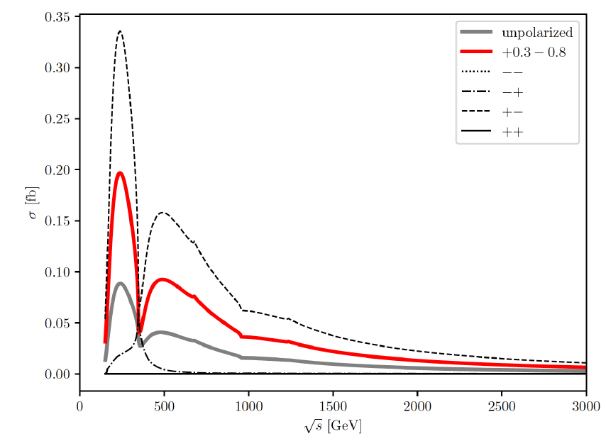
Figure 3: $\sigma(e^{+}e^{-}\to h\gamma)$. Loop induced (i.e. leading two-loop corrected) cross sections are shown with parameters chosen according to $\mathcal{S}$2 (see Tab. 1) as a function of $\sqrt{s}$ for various polarizations (see text).

3.4 The process $e^{+}e^{-}\to h\gamma$: stop sector dependance

In Fig. 4 we show the results for the process $e^{+}e^{-}\to h\gamma$ (no complex parameters) in $\mathcal{S}$2 in the $M_{Q_{3}}$–$M_{U_{3}}$ plane for $A_{t}=2200\,\,\mathrm{GeV},2600\,\,\mathrm{GeV},3000\,\,\mathrm{GeV}$ in the upper, middle, lower row, respectively (see Ref. [44] for details). The left column shows the MSSM production cross section, while the middle column indicates the SM cross section, where at each point the Higgs boson mass has been adjusted. Here it should be noted that the color code slightly changes from left to middle column. In all the colored area the light ${\cal CP}$-even Higgs boson mass is found in the interval $122\,\,\mathrm{GeV}\ldots 128\,\,\mathrm{GeV}$ (using FeynHiggs version 2.13.0). The cross section varies by around $\sim 5\%$, which can partly be attributed to the variation of $M_{h}$.

In order to disentangle these effects, the right most column shows the differences between the MSSM and SM cross section, i.e. the genuine SUSY loop effects on the cross section calculation. Those are found at the level of $\sim 1.5\%$ to $\sim 3.5\%$, where the smallest (largest) difference is found for small $M_{Q_{3}}$ and small (large) $M_{U_{3}}$. Overall, the variation in the cross section due to SUSY loop effects, despite being a loop induced process, will likely remain too small to be observable at future $e^{+}e^{-}$ colliders such as ILC, CLIC, FCC-ee or CEPC.

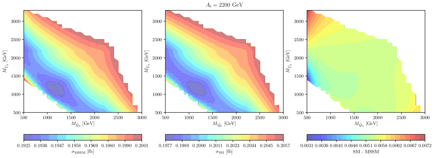
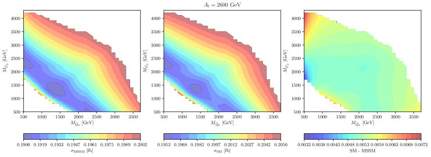
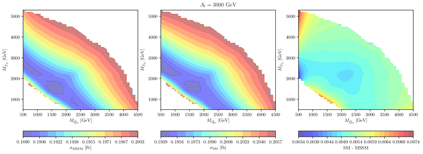
Figure 4: $\sigma(e^{+}e^{-}\to h\gamma)$. Loop induced (i.e. leading two-loop corrected) cross sections are shown with parameters chosen according to $\mathcal{S}$2 (see Tab. 1) in the $M_{Q_{3}}$–$M_{U_{3}}$ plane for $A_{t}=2200\,\,\mathrm{GeV},2600\,\,\mathrm{GeV},3000\,\,\mathrm{GeV}$ in the upper, middle, lower row, respectively. The left (middle) column shows the MSSM (SM) production cross section, while the right column indicates the difference between the two (see text).

Acknowledgements

The work of F.A. was supported by the Spanish Ministry of Science and Innovation via an FPU grant. The work of S.H. was supported in part by the MEINCOP (Spain) under contract FPA2016-78022-P and in part by the AEI through the grant IFT Centro de Excelencia Severo Ochoa SEV-2016-0597. The work of S.H. was furthermore supported in part by the Spanish Agencia Estatal de Investigación (AEI), in part by the EU Fondo Europeo de Desarrollo Regional (FEDER) through the project FPA2016-78645-P, in part by the “Spanish Red Consolider MultiDark” FPA2017-90566-REDC.

References

-
[1]
H. Nilles,
Phys. Rept. 110 (1984) 1;
R. Barbieri, Riv. Nuovo Cim. 11 (1988) 1. - [2] H. Haber, G. Kane, Phys. Rept. 117 (1985) 75.
- [3] J. Gunion, H. Haber, Nucl. Phys. B 272 (1986) 1.
-
[4]
A. Pilaftsis,
Phys. Rev. D 58 (1998) 096010
[arXiv:hep-ph/9803297];
A. Pilaftsis, Phys. Lett. B 435 (1998) 88 [arXiv:hep-ph/9805373]. - [5] D. Demir, Phys. Rev. D 60 (1999) 055006 [arXiv:hep-ph/9901389].
- [6] A. Pilaftsis and C. Wagner, Nucl. Phys. B 553 (1999) 3 [arXiv:hep-ph/9902371].
- [7] S. Heinemeyer, Eur. Phys. J. C 22 (2001) 521 [arXiv:hep-ph/0108059].
- [8] S. Heinemeyer, O. Stål and G. Weiglein, Phys. Lett. B 710 (2012) 201 [arXiv:1112.3026 [hep-ph]].
- [9] G. Aad et al. [ATLAS Collaboration], Phys. Lett. B 716 (2012) 1 [arXiv:1207.7214 [hep-ex]].
- [10] S. Chatrchyan et al. [CMS Collaboration], Phys. Lett. B 716 (2012) 30 [arXiv:1207.7235 [hep-ex]].
- [11] G. Aad et al. [ATLAS and CMS Collaborations], Phys. Rev. Lett. 114 (2015) 191803 [arXiv:1503.07589 [hep-ex]].
- [12] H. Baer et al., The International Linear Collider Technical Design Report - Volume 2: Physics, arXiv:1306.6352 [hep-ph].
- [13] G. Moortgat-Pick et al., Eur. Phys. J. C 75 (2015) 8, 371 [arXiv:1504.01726 [hep-ph]].
-
[14]
L. Linssen, A. Miyamoto, M. Stanitzki and H. Weerts,
arXiv:1202.5940 [physics.ins-det];
H. Abramowicz et al. [CLIC Detector and Physics Study Collaboration], Physics at the CLIC Linear Collider – Input to the Snowmass process 2013, arXiv:1307.5288 [hep-ex];
P. Burrows et al. [CLICdp and CLIC Collaborations], CERN Yellow Rep. Monogr. 1802 (2018) 1 [arXiv:1812.06018 [physics.acc-ph]]. -
[15]
A. Abada et al. [FCC Collaboration],
Eur. Phys. J. C 79 (2019) no.6, 474;
A. Abada et al. [FCC Collaboration], Eur. Phys. J. ST 228 (2019) no.2, 261. -
[16]
J. Guimarães da Costa et al. [CEPC Study Group],
arXiv:1811.10545 [hep-ex];
F. An et al., Chin. Phys. C 43 (2019) no.4, 043002 [arXiv:1810.09037 [hep-ex]]. - [17] K. Williams, H. Rzehak, and G. Weiglein, Eur. Phys. J. C 71 (2011) 1669 [arXiv:1103.1335 [hep-ph]].
- [18] S. Heinemeyer and C. Schappacher, Eur. Phys. J C 75 (2015) 5, 198 [arXiv:1410.2787 [hep-ph]].
- [19] S. Heinemeyer and C. Schappacher, Eur. Phys. J C 75 (2015) 5, 230 [arXiv:1503.02996 [hep-ph]].
- [20] S. Heinemeyer, W. Hollik and G. Weiglein, Eur. Phys. J. C 16 (2000) 139 [arXiv:hep-ph/0003022].
-
[21]
R. Hempfling,
Phys. Rev. D 49 (1994) 6168;
L. Hall, R. Rattazzi and U. Sarid, Phys. Rev. D 50 (1994) 7048 [arXiv:hep-ph/9306309];
M. Carena, M. Olechowski, S. Pokorski and C. Wagner, Nucl. Phys. B 426 (1994) 269 [arXiv:hep-ph/9402253];
M. Carena, D. Garcia, U. Nierste and C. Wagner, Nucl. Phys. B 577 (2000) 577 [arXiv:hep-ph/9912516]. - [22] D. Noth and M. Spira, Phys. Rev. Lett. 101 (2008) 181801 [arXiv:0808.0087 [hep-ph]]; JHEP 1106 (2011) 084 [arXiv:1001.1935 [hep-ph]].
- [23] V. Barger, M. Berger, A. Stange and R. Phillips, Phys. Rev. D 45 (1992) 4128.
- [24] S. Heinemeyer and W. Hollik, Nucl. Phys. B 474 (1996) 32 [arXiv:hep-ph/9602318].
- [25] W. Hollik and J. Zhang, Phys. Rev. D 84 (2011) 055022 [arXiv:1109.4781 [hep-ph]].
-
[26]
A. Bredenstein, A. Denner, S. Dittmaier and M. Weber,
Phys. Rev. D 74 (2006) 013004
[arXiv:hep-ph/0604011];
JHEP 0702 (2007) 080
[arXiv:hep-ph/0611234];
A. Bredenstein, A. Denner, S. Dittmaier, A. Mück and M. Weber,
see: omnibus.uni-freiburg.de/~sd565/programs/prophecy4f/prophecy4f.html . - [27] M. Frank, T. Hahn, S. Heinemeyer, W. Hollik, H. Rzehak and G. Weiglein, JHEP 0702 (2007) 047 [arXiv:hep-ph/0611326].
-
[28]
F. Domingo, S. Heinemeyer, S. Paßehr and G. Weiglein,
Eur. Phys. J. C 78 (2018) no.11, 942
[arXiv:1807.06322 [hep-ph]];
F. Domingo and S. Paßehr, Eur. Phys. J. C 79 (2019) no.11, 905 [arXiv:1907.05468 [hep-ph]]. -
[29]
S. Heinemeyer, W. Hollik and G. Weiglein,
Comput. Phys. Commun. 124 (2000) 76
[arXiv:hep-ph/9812320];
T. Hahn, S. Heinemeyer, W. Hollik, H. Rzehak and G. Weiglein, Comput. Phys. Commun. 180 (2009) 1426, see: www.feynhiggs.de . - [30] S. Heinemeyer, W. Hollik and G. Weiglein, Eur. Phys. J. C 9 (1999) 343 [arXiv:hep-ph/9812472].
- [31] G. Degrassi, S. Heinemeyer, W. Hollik, P. Slavich and G. Weiglein, Eur. Phys. J. C 28 (2003) 133 [arXiv:hep-ph/0212020].
- [32] T. Hahn, S. Heinemeyer, W. Hollik, H. Rzehak and G. Weiglein, Phys. Rev. Lett. 112 (2014) 141801 [arXiv:1312.4937 [hep-ph]].
-
[33]
H. Bahl and W. Hollik,
Eur. Phys. J. C 76 (2016) no.9, 499
[arXiv:1608.01880 [hep-ph]];
H. Bahl, S. Heinemeyer, W. Hollik and G. Weiglein, Eur. Phys. J. C 78 (2018) no.1, 57 [arXiv:1706.00346 [hep-ph]];
H. Bahl, T. Hahn, S. Heinemeyer, W. Hollik, S. Paßehr, H. Rzehak and G. Weiglein, Comput. Phys. Commun. 249 (2020) 107099 [arXiv:1811.09073 [hep-ph]]. - [34] S. Heinemeyer and C. Schappacher, Eur. Phys. J. C 76 (2016) no.4, 220 [arXiv:1511.06002 [hep-ph]].
- [35] S. Heinemeyer and C. Schappacher, Eur. Phys. J. C 76 (2016) no.10, 535 [arXiv:1606.06981 [hep-ph]].
- [36] S. Heinemeyer and C. Schappacher, Eur. Phys. J. C 78 (2018) no.7, 536 [arXiv:1803.10645 [hep-ph]].
- [37] S. Heinemeyer and C. Schappacher, PoS LL 2018 (2018) 056 [arXiv:1807.04009 [hep-ph]].
- [38] S. Heinemeyer and C. Schappacher, Eur. Phys. J. C 77 (2017) no.9, 649 [arXiv:1704.07627 [hep-ph]].
- [39] S. Kanemura, K. Mawatari and K. Sakurai, Phys. Rev. D 99 (2019) no.3, 035023 [arXiv:1808.10268 [hep-ph]].
-
[40]
J. Küblbeck, M. Böhm and A. Denner,
Comput. Phys. Commun. 60 (1990) 165;
T. Hahn, Comput. Phys. Commun. 140 (2001) 418 [arXiv:hep-ph/0012260];
T. Hahn and C. Schappacher, Comput. Phys. Commun. 143 (2002) 54 [arXiv:hep-ph/0105349].
Program, user’s guide and model files are available via: www.feynarts.de . - [41] T. Fritzsche, T. Hahn, S. Heinemeyer, F. von der Pahlen, H. Rzehak and C. Schappacher, Comput. Phys. Commun. 185 (2014) 1529 [arXiv:1309.1692 [hep-ph]].
- [42] T. Hahn and M. Pérez-Victoria, Comput. Phys. Commun. 118 (1999) 153 [arXiv:hep-ph/9807565].
-
[43]
J. Frère, D. Jones and S. Raby,
Nucl. Phys. B 222 (1983) 11;
M. Claudson, L. Hall and I. Hinchliffe, Nucl. Phys. B 228 (1983) 501;
C. Kounnas, A. Lahanas, D. Nanopoulos and M. Quiros, Nucl. Phys. B 236 (1984) 438;
J. Gunion, H. Haber and M. Sher, Nucl. Phys. B 306 (1988) 1;
J. Casas, A. Lleyda and C. Muñoz, Nucl. Phys. B 471 (1996) 3 [arXiv:hep-ph/9507294];
P. Langacker and N. Polonsky, Phys. Rev. D 50 (1994) 2199 [arXiv:hep-ph/9403306];
A. Strumia, Nucl. Phys. B 482 (1996) 24 [arXiv:hep-ph/9604417]. - [44] F. Arco, master thesis “The Higgs boson in the MSSM and the Higgs-photon production in future linear colliders”, IFT (UAM/CSIC), Madrid, Spain, September 2018.
- [45] T. Barklow, et al. arXiv:1506.07830 [hep-ex].