Trimming the Sail: A Second-order Learning Paradigm for Stock Prediction

Abstract

Nowadays, machine learning methods have been widely used in stock prediction. Traditional approaches assume an identical data distribution, under which a learned model on the training data is fixed and applied directly in the test data. Although such assumption has made traditional machine learning techniques succeed in many real-world tasks, the highly dynamic nature of the stock market invalidates the strict assumption in stock prediction. To address this challenge, we propose the second-order identical distribution assumption, where the data distribution is assumed to be fluctuating over time with certain patterns. Based on such assumption, we develop a second-order learning paradigm with multi-scale patterns. Extensive experiments on real-world Chinese stock data demonstrate the effectiveness of our second-order learning paradigm in stock prediction.

1 Introduction

Stock prediction, with the aim at predicting future price trend of stocks, is one of the most important fundamental techniques for stock investment Preethi and Santhi (2012). To facilitate stock prediction, traditional quantitative investment approaches usually recognize some trading indicators and then conduct predictions based on these indicators Suh et al. (2004). Recently, substantial machine learning techniques have been introduced into stock prediction, since its strong capability in automatically identifying underlying patterns over indicators from the historical data with little human knowledge Patel et al. (2015); Cervelló-Royo et al. (2015).

Formally, a typical machine learning approach intends to learn a parameterized function $F_{\theta}$, mapping the input features $X$, i.e., various trading indicators, into the output target $Y$, i.e., the stock future trend. While recent years have witnessed a variety of machine learning techniques with different forms of $F_{\theta}$, such as Linear Regression Zhang et al. (2014), Random Forest Khaidem et al. (2016), Neural Networks  Zhang et al. (2017); Nelson et al. (2017); Fischer and Krauss (2018), etc., typical learning-based approaches for stock prediction feel pain when facing the dynamic nature of the stock market.

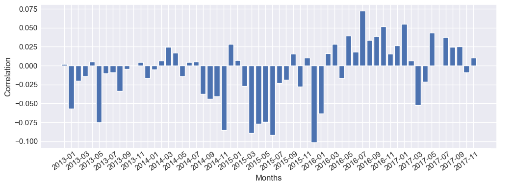
Figure 1: The correlation between the market value of stocks and returns in each month of Chinese market from 2013 to 2017.

Specifically, traditional machine learning approaches usually assume an identical data distribution (i.d.) $P(X,Y)$. Thus, after obtaining the optimal $F_{\theta}$ on the training data, the corresponding parameters are fixed and applied directly in the test data. We refer to such assumption as the first-order i.d. assumption. Unfortunately, due to the highly dynamic nature of stock market, the data distribution $P(X,Y)$ usually varies over time $t$. Figure  1 shows the correlations between the market values of stocks and returns in different months of Chinese market. As we can see, the market value is negatively correlated with the future return before the year of 2016, while positively after 2016. Thus, it is hard to apply a fixed model to achieve accurate prediction on before and after 2016 simultaneously. In other words, the optimal first-order model $F_{\theta}$ can shift drastically along with different time periods. Therefore, it is fairly important to consider the change of data distribution over time in stock prediction task.

To seek sustaining accurate stock prediction under the critical challenge of non-identical data distribution, a straightforward method is to employ the rotation learning paradigm, which keeps updating new models $F_{\theta_{[t-\Delta,t]}}$ by rotating the training procedure using merely the most recent data within the certain time window $[t-\Delta,t]$. Nevertheless, the rotation learning paradigm still suffers from a couple of disadvantages. The most important one is that, even though the rotation learning paradigm has attempted to bridge the gap in terms of the data distribution between the training and the testing data, it cannot handle sudden distribution altering. On the other hand, the distribution variation of financial market is not completely intractable. Many studies have demonstrated some variation patterns on the financial market. For example, the famous report Merrill Lynch Investment Clock Lynch (2004) claims that the market returns vary over a time loop. Numerous theories of economic cycle have been proposed by many financial professors Lucas (1980); Choe et al. (1993); Næs et al. (2011). Motivated by this, we propose second-order i.d. assumption.

Table 1: Trading indicators and their categories with respective calculation formulas, where $p_{open}(t)$, $p_{close}(t)$, $p_{high}(t)$ and $p_{low}(t)$ denote the opening price, closing price, highest price and lowest price at time $t$, and $m$ is the size of sliding time window.

Indicators	Calculation Formula
$KLEN(t)$	$(p_{close}(t)-p_{open}(t))/(p_{open}(t))$
$KUP(t)$	$[p_{high}(t)-\max(p_{open}(t),p_{close}(t))]/p_{open}(t)$
$KLOW(t)$	$[\min(p_{open}(t),p_{close}(t))-p_{low}(t)]/p_{open}(t)$
$MA_{m}(t)$	$\frac{1}{m}\sum_{j=0}^{j=m-1}p_{close}(t-j)$
$EMA_{m}(t)$	$[p_{close}(t)-EMA_{m}(t-1)]\times\frac{2}{m+1}+EMA_{m}(t-1)$
$Bias_{m}(t)$	$p_{close}(t)-\frac{1}{m}\sum_{j=0}^{j=m-1}p_{close}(t-j)$
$ROC_{m}(t)$	$(p_{close}(t)-p_{close}(t-m))/p_{close}(t-m)$

• Second-order i.d. assumption. We assume that the data distribution $P(X,Y)$ is fluctuating over time with certain patterns. That is, for each time period $t$, the optimal parameter $\theta_{t}$ of $F_{\theta_{t}}$ can be modeled by a second-order model $G$. Formally, $\theta_{t}=G(\theta_{<t})$.

Note that the first-order method can be seen as a special case under second-order i.d. assumption when the mapping $G$ is an identity function. Based on the second-order i.d. assumption, we propose a novel learning paradigm which attempts to learn the model $G$ from history, and thus derive the proper first-order model to predict the future stock trends more accurately.

Our contributions in this paper can be summarized as:

• We identify the first-order i.d. assumption in typical machine learning tasks, which is invalid in stock prediction due to the highly dynamic nature of stock market.

• We introduce the second-order i.d. assumption and propose a novel learning paradigm which is able to capture the dynamics of stock market for more accurate prediction.

• We conduct extensive experiments on Chinese stock market for more than 2000 stocks over 5 years. Empirical results demonstrate that our paradigm significantly outperforms the first-order methods as well as the rotation learning methods in the stock prediction.

The rest of the paper is organized as follows. We first present several preliminaries in Section 2. Then, in Section 3, we present our second-order learning paradigm in details. Finally, we demonstrate the experiment results, related work and conclusion in Section 4, 5 and 6.

2 Preliminary

2.1 Trading Indicator

Substantial previous works use trading indicators as the input $X$ of the first-order model $F$ Savin et al. (2006); Kamijo and Tanigawa (1990); Brock et al. (1992). Table 1 shows some popular indicators with their respective calculation formulas. Different indicators reflect distinct aspects of trading patterns. Candlestick indicators, such as “KLEN”, tend to represent trading patterns over short periods of time, usually a few days or a few trading sessions. Trend indicators, such as “MA”, measure the direction and strength of a trend, using some forms of price averaging. Momentum indicators, such as “ROC”, identify the speed of price movement by comparing the current closing price to the previous closes.

2.2 Indicator Effectiveness

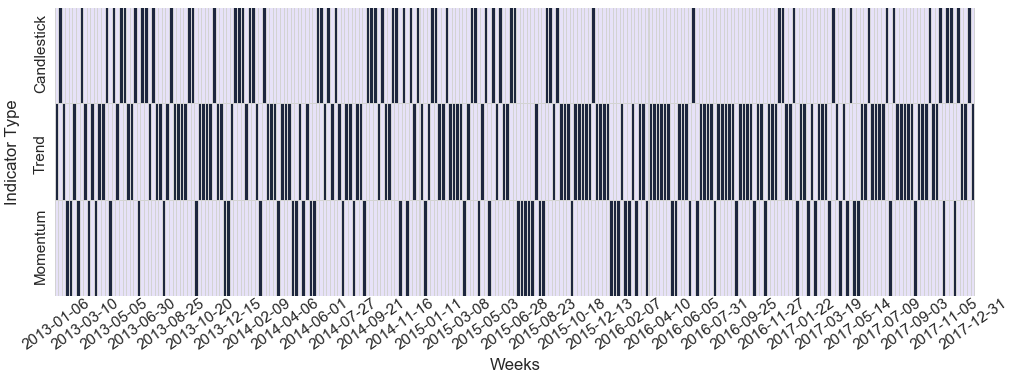
Figure 2: The most effective indicator among the three types (“candlestick”, “trend” and “momentum”) in weeks from 2013 to 2017. Each column corresponds to a week, and each row corresponds to a type of indicators. The dark color represents the highest IC value, which means the corresponding type of indicator is the most effective for the stock prediction.

In the financial field, experts usually evaluate the effectiveness of indicators by Information Coefficient (IC) . The indicator effectiveness reflects the state of the current market. More effective indicators can guide us to a more accurate prediction. Existing first-order methods assume that the effectiveness of indicators stays constant. Thus, once the model finishes training, the corresponding parameters will be fixedly used on any future data. However, as we mentioned, due to the highly dynamic nature of the stock market, indicator effectiveness is changing over time. Figure  2 shows the change of effectiveness of three types of trading indicators from 2013 to 2017. As we can see, the most effective type does not stay constant but frequent altering, which limits the performance of first-order methods and rotation learning methods. In general, the momentum indicator demonstrates cyclic effective. The trend indicator tends to be more effective while the candlestick indicator is less after the year of 2016. There could be much more complicated patterns of the effectiveness variation which cannot be apparently observed. Therefore, we resort to discover such patterns automatically with a second-order learning paradigm.

3 Second-order Learning Paradigm

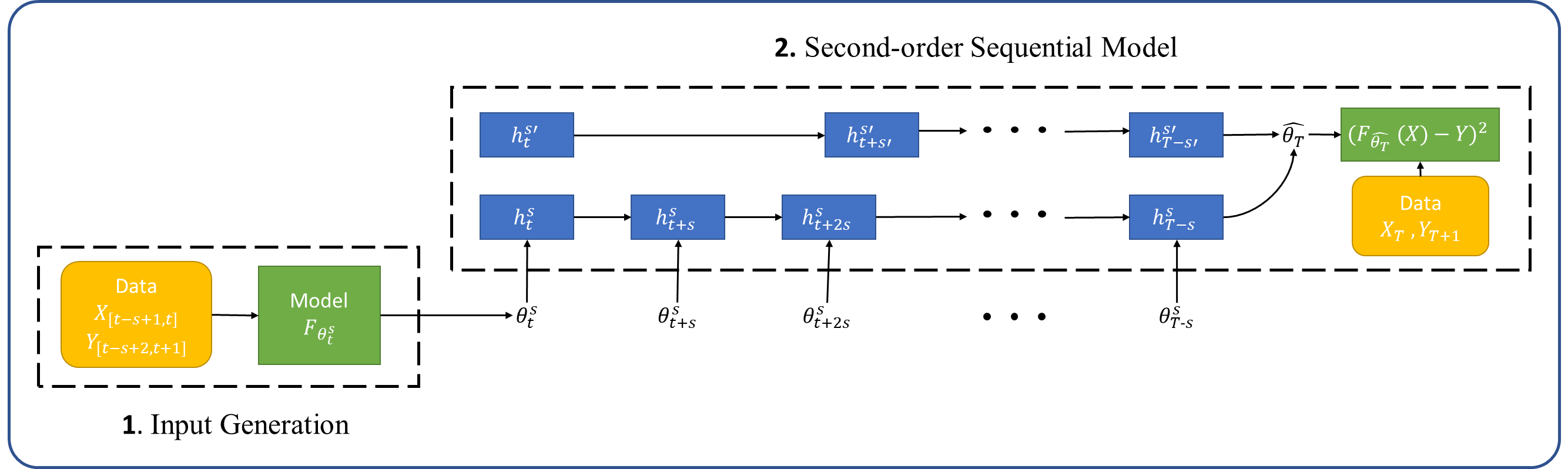
Figure 3: The framework of second-order learning paradigm. Our framework consists of two parts. 1. Input Generation: learning parameter $\theta_{t}$ for prediction model $F_{\theta_{t}}(X)$ from historical data, as the input of the second part. 2. Second-order Sequential Model: predicting optimal model parameter $\theta_{T}$ at time step $T$ with diverse time scale in a unified fashion.

In this section, we describe our second-order learning paradigm in detail. Our proposed paradigm contains two parts. In the first part, we partition the historical data into several periods with multiple time scales. Then, for each time period $t$, we obtain the optimal parameters for the corresponding first-order model $F$. The obtained parameter sequence is used as the input of the second part. Next, in the second part, we use a second-order sequential model $G$ to learn how the optimal parameters $\theta_{t}$ varies over time using model $G$, and thus predict the future stock trend.

3.1 Input Generation

We first present how to generate parameter $\theta_{t}$, i.e., the input of our second-order model. To capture the evolving patterns of stock market, for each time period $t$, we train a first-order model $F_{\theta_{t}}$ which generalizes the market state at time $t$. Despite there are many potential types of parameterized function $F_{\theta}$, in this paper, we focus on the linear model because: (1) The data quantity during a small time period is very limited. Thus, the non-linear models such as Decision Tree or Neural Network are prone to overfit the data. (2) For the linear model, each parameter has a well-defined economic meaning. A linear model can be written as

$$F_{\theta}(X)=\mathbf{w}X+b,$$ (1)

where $\theta=(\mathbf{w},b)$. A positive/negative value of weight $w_{i}$ implies that $X_{i}$ yields a positive/negative correlation with the stock trend. In the meantime, a larger absolute value of $w_{i}$ usually indicates a more effective trading indicator $X_{i}$. Such interpretability is very critical in the financial domain and helps people understand the market dynamics.

In this paper, we actually partition the historical data with multiple time scales. Then, the parameters can be obtained by training the model for each time scale. For the $t$-th time period under time scale $s$, we obtain the parameter vector $\theta_{t}^{s}$ using the historical data $X_{[t-s+1,t]}$ and the corresponding label $Y_{[t-s+2,t+1]}$. Intuitively, the sequence of parameters in macro-scale reflects the long-term trend of market state, while micro-scale reflects the short-term trend.

3.2 Second-order Sequential Model

In the second part, we propose a second-order sequential model to learn the evolving market trends and predict future stock prices. Due to the temporal dynamics in the stock market, we take advantages of the LSTM modeling  Hochreiter and Schmidhuber (1997), which has been widely used to capture the temporal dependencies in the input sequences. In our case, recall that we obtained multiple parameter sequences with different time scales in the first part. For the $t$-th period under the time scale $s$, we have that

$$h_{t}^{s}=\mathrm{LSTM}(h_{t-s}^{s},\theta_{t}^{s}),$$ (2)

where $h_{t}^{s}$ is the corresponding “hidden vector” which represents the temporal patterns before $t$. For different time scales, since the macro and micro scales indicate different market trends, we use the attention mechanism to combine the hidden states of different time scales, i.e.,

$$\hat{\theta}_{T}=\sum_{s}\chi(\alpha^{s}h_{T-s}),$$ (3)

where $\chi$ is a fully-connected layer transforming the hidden vector to the predicted parameter, and $\alpha^{s}\in R$ is the attention weight of the time scale $s$ which is automatically learned by the model. The output $\hat{\theta}_{T}$ corresponds to the first-order parameter estimated by the second-order sequential model at the future period $T$. Thus, the future stock trend can be modeled by the function $F_{\hat{\theta}_{T}}$.

To train our paradigm, one feasible way is to first obtain the “ground-truth” parameter at time $T$ by $(X_{T},Y_{T})$ with a first-order model. Then we minimize the gap between the ground-truth and the estimated parameter $\hat{\theta}_{T}$. However, here, note that the “ground-truth” parameter obtained by the first-order model is also an empirical estimation. Directly learning such “ground-truth” would cause the error accumulation. Instead, we directly optimize the final prediction and the stock trend. The loss function $\mathcal{L}$ can be defined by

$$\mathcal{L}=(F_{\hat{\theta}_{T}}(X_{T})-Y_{T})^{2}.$$ (4)

We display the whole framework of the second learning paradigm in Figure  3 and formulate the process of the second-order sequential model in Algorithm 1.

Algorithm 1 Stock prediction by second-order sequential model.

Input: Training set $D_{1}=\{(X_{t},Y_{t+1})|t\in[0,T_{a}-1]\}$.
Testing set $D_{2}=\{(X_{t},Y_{t+1})|t\in[T_{a},T_{b}]\}$.
Time-scale set $S$. Episode number $E$.
Second-order sequential model $G_{\Phi}$ with $K$ time steps.
Output: Stock trends $O$.

Training second-order sequential model $G$.

1:Initialize $G_{\Phi}$;

2:Generate parameters $\Theta=\{\theta^{s}_{t}|s\in S,t\in[0,T_{a}-1]\}$ from $D_{1}$;

3:Construct $G$’s training set $\{(X^{g}_{t},Y_{t+1})|t\in[0,T_{a}-1]\}$ where $X_{t}^{g}=\{\theta^{s}_{t-ks},X_{t}|s\in S,k\in[1,K]\}$;

4:for $e\leftarrow 1$ to $E$ do

5:     $\Phi\leftarrow\Phi-\nabla_{\Phi}(G(X_{t}^{g})-Y_{t+1})^{2}$;

Predicting by second-order sequential model $G$.

1:Prediction results $O\leftarrow\emptyset$;

2:for $t\leftarrow T_{a}$ to $T_{b}$ do

3:     $X^{g}_{t}=\{\theta^{s}_{t-ks},X_{t}|s\in S,k\in[1,K]\}$;

4:     $\hat{Y}_{{t+1}}=G_{\Phi}(X^{g}_{t})$;

5:     $O\leftarrow O\cup\{\hat{Y}_{t+1}\}$;

6:     Generate parameters $\Theta_{t}=\{\theta^{s}_{t}|s\in S\}$;

7:     $\Theta\leftarrow\Theta\cup\Theta_{t}$;

8:return $O$;

4 Experiments

4.1 Experimental Setup

Data Set. We evaluate our method on the real-world stock data of the Chinese market from 2013 to 2017 in daily frequency . There are more than 2000 stocks in total, covering the vast majority of Chinese stocks. In order to model the market trend, we filter out several “bad” stocks which are under suspended trading status for more than 10% of trading days. After that, there are totally 1246 stocks that are used in our experiments. Furthermore, we follow the previous study  Kakushadze (2016) to compute totally 101 trading indicators as the input of the first-order model.

In the following experiments, we use the stock data from 2013 to 2016 for training and validation while use the data of 2017 for testing. In order to validate the models in different market states, the training set and validation set are randomly extracted from the whole period from 2013 to 2016. Specifically, we randomly sample $1/10$ data from this period as the validation set, while the other $9/10$ as the training set.

Compared Methods. To evaluate the effectiveness of our models, we compare the following methods:

• First-order Learning Paradigm for Linear Model ($\mathrm{Lin}$): The method is the vanilla combination with inputs. It learns static model parameters on the training set, then predicts the future trend of stocks on the test data directly.

• Rotation Learning for Linear Model with Window Size w ($\mathrm{RoT}$-w): This method keeps generating the new model by rotation using merely the recent data within a certain time window, where $w$ is the corresponding window size.

• Second-order Sequential Model with s-scale ($\mathrm{Sec}$-s): This approach is a special case of our proposed model, where we only use a single scale $s$. We introduce this special case to demonstrate the effectiveness of the multi-scale design.

• Multi-scale Second-order Sequential Model ($\mathrm{multi}$-$\mathrm{Sec}$): This is our proposed model which captures how the optimal prediction model evolves over time with multi-scale second-order patterns.

In this paper, we consider the time scale in days, for example, $\mathrm{Sec}$-1 denotes the second-order sequential model with 1-day scale. $\mathrm{RoT}$-60 uses 60-day window to train the model. Furthermore, $\mathrm{multi}$-$\mathrm{Sec}$ combines the patterns with respect to several scales, including 1-day, 5-day (1 week), 10-day (2 weeks) and 20-day (1 month) in this paper.

Evaluation Metrics. To compare the stock prediction methods, we evaluate the performance of top-$K$ stocks sorted by the predicted daily returns in descending order. We adopt the most widely used metrics, Annualized Return (AR) and Sharpe Ratio (SHR) to evaluate the performance of stock prediction, i.e.,

• Annualized Return (AR) is a common profit indicator in finance, calculated by the mean return of selected $K$ stocks in a $l$-day period to one year. Specifically,

  $$AR@K=\frac{1}{K}\sum_{d\in[1,l]}\sum_{i\in\Lambda_{d}}r^{i}_{d}\times\frac{365}{l},$$ (5)

  where $\Lambda_{d}$ is the collection of selected top-$K$ stocks in the $d$-th day, and $r^{i}_{d}$ represents the return of stock $i$ in the $d$-th day.

• Sharpe Ratio Sharpe (1966) (SHR) is a risk-adjusted profit measure that computes the return per unit of deviation. In a formal definition,

  $$SHR@K=\frac{1}{l}\sum_{d\in[1,l]}\frac{\frac{1}{K}\sum_{i\in\Lambda_{d}}(r^{i}_{d}-\bar{r}_{d})}{\sqrt{var(\{r^{i}_{d}|i\in\Lambda_{d}\})}},$$ (6)

  where $\bar{r}_{d}$ is the average return of the market in the $d$-th day. Thus, SHR is positively related to the return and negatively related to the risk of a strategy.

To evaluate methods from various aspects, we respectively study the performance in top-$\{10,20,50\}$ strategies.

Hyperparameter Settings. We employ the grid search to select the optimal hyperparameters regarding MSE on the validation sets for all methods. For LSTM parts of the models, we tune the number of LSTM cells within {5, 10, 20}, initialize the forget bias within {0, 0.5, 1} and tune the size of the hidden vector within {64, 128}.

4.2 Results

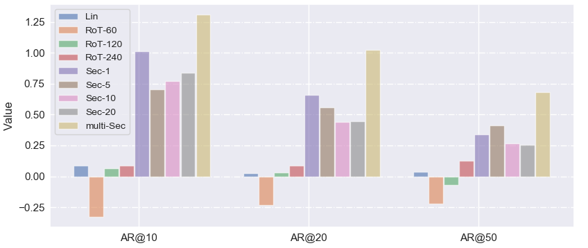
Figure 4: The performance comparison on AR@10, 20, 50 among $\mathrm{Lin}$, $\mathrm{RoT}$, $\mathrm{Sec}$ and $\mathrm{multi}$-$\mathrm{Sec}$.

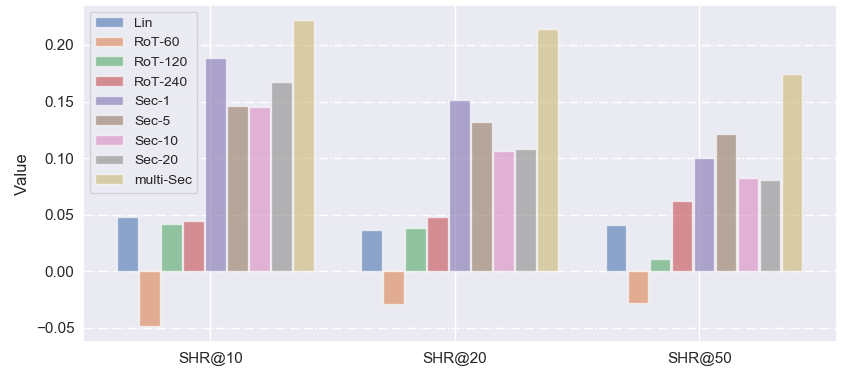
Figure 5: The performance comparison on SHR @10, 20, 50 among $\mathrm{Lin}$, $\mathrm{RoT}$, $\mathrm{Sec}$ and $\mathrm{multi}$-$\mathrm{Sec}$.

Main Results. Figure 4 and 5 present the results among $\mathrm{Lin}$, $\mathrm{RoT}$, $\mathrm{Sec}$, and $\mathrm{multi}$-$\mathrm{Sec}$ on the test set. In general, $\mathrm{Sec}$ and $\mathrm{multi}$-$\mathrm{Sec}$ have significantly better performance than the other methods, which demonstrates that it is necessary to propose the second-order learning paradigm. Although $\mathrm{RoT}$ can update the first-order model dynamically, it is still much worse than our algorithm, which indicates that it is not enough to obtain a concrete prediction only by rotation learning. In terms of different scales of the proposed $\mathrm{Sec}$, $\mathrm{Sec}$-1 performs the best on the top-10 and top-20 investment while $\mathrm{Sec}$-5 brings the most profit on the top-50 investment, which states that different time scales brings different profit in the stock market. By combining different time scales, our proposed $\mathrm{multi}$-$\mathrm{Sec}$ achieves the best performance.

Rotation Learning Paradigm. In Figures 4 and 5, $\mathrm{RoT}$-60 generates a money-losing investment, while $\mathrm{Lin}$, $\mathrm{Sec}$, and $\mathrm{multi}$-$\mathrm{Sec}$ can bring less or more profit. This is mainly due to that the rotation learning paradigm pays much attention on the recent data. However, since the stock market is highly dynamic, the method will suffer from the sudden distribution altering in the stock market. Enlarging the rotation window size alleviate this issue. Especially, in most cases, $\mathrm{RoT}$-240 outperforms $\mathrm{Lin}$ and $\mathrm{RoT}$ with the other window sizes.

Single-scale vs. Multi-scale. As Figures 4 and 5 show, $\mathrm{multi}$-$\mathrm{Sec}$ significantly outperforms the single scale models. It demonstrates that diverse information from the multi-scale market states is beneficial to the stock prediction. In addition, the more stocks are invested, the more advantages are generated by the multi-scale design: $\mathrm{multi}$-$\mathrm{Sec}$ is larger 0.0337, 0.0624 and 0.0742 than $\mathrm{Sec}$-1 on respectively SHR@$10,20,50$. This indicates that multi-scale information is especially useful to the diversified investment.

$\alpha^{s}$ Value. In order to study the contribution made by each scale, we print the magnitude of weight $\alpha^{s}$ in each scale: 0.1357 on 1-day scale, 0.1393 on 5-day scale, 0.1353 on 10-day scale and 0.2290 on 20-day scale. There are a couple of observations from $\alpha^{s}$ distribution: the 1-day, 5-day and 10-day scale have similar absolute weights, which indicates that the three scales contains similar information. In the meantime, the distinctly higher weight of 20-day scale implies that the 20-day scale brings very different information from the other scales, and is precious for stock prediction.

Case Studies. To compare the single-scale and multi-scale design, Table 2 shows the predicted weight of trading indicator MA₁₀ by $\mathrm{Sec}$ with different scales and $\mathrm{multi}$-$\mathrm{Sec}$. As the table shows, $\mathrm{multi}$-$\mathrm{Sec}$ and ground-truth have similar second-order trends with co-directional weights (-+-+-). This illustrates that our proposed $\mathrm{multi}$-$\mathrm{Sec}$ can model the reversal trend of second-order sequence which cannot be captured by rotation learning paradigm because it assumes the same data distribution between the recent data and the predicted data. Furthermore, $\mathrm{Sec}$ in distinct scales have different second-order patterns, for example, the trend of $\mathrm{Sec}$-1 is (down, up, up, down) from 2017/03/27 to 2017/03/31, while $\mathrm{Sec}$-20 corresponds to (up, down, down up).

Table 2: The predicted weight of indicator MA₁₀ in different scale.

Date	Ground-truth	Sec-1	Sec-5
2017-03-27	-0.0226	0.0076	0.0486
2017-03-28	0.1858	0.0049	0.0478
2017-03-29	-0.0120	0.0070	0.0409
2017-03-30	0.0633	0.0307	0.0046
2017-03-31	-0.0254	0.0198	0.0288
Date	Sec-10	Sec-20	multi-Sec
2017-03-27	0.0363	0.0078	-0.0408
2017-03-28	0.0307	0.0398	0.0031
2017-03-29	0.0075	0.0334	-0.0196
2017-03-30	0.0088	0.0054	0.0083
2017-03-31	0.0346	0.0078	-0.0277

4.3 Market Trading Simulation

To further evaluate the effectiveness of our proposed models, we conduct the back-testing by simulating the stock trading for the test dataset. Our estimation strategy conducts trading in the daily frequency. Given a certain principal at the beginning of the back-testing, investors invest in the top-$K$ stocks with the highest predicted return in each day. The selected stocks are held for one day. The cumulative profit without consideration of transaction cost will be invested in the next trading day. We also calculate the average return on the stock market by evenly holding every stock as the baseline, indicating the overall market trend.

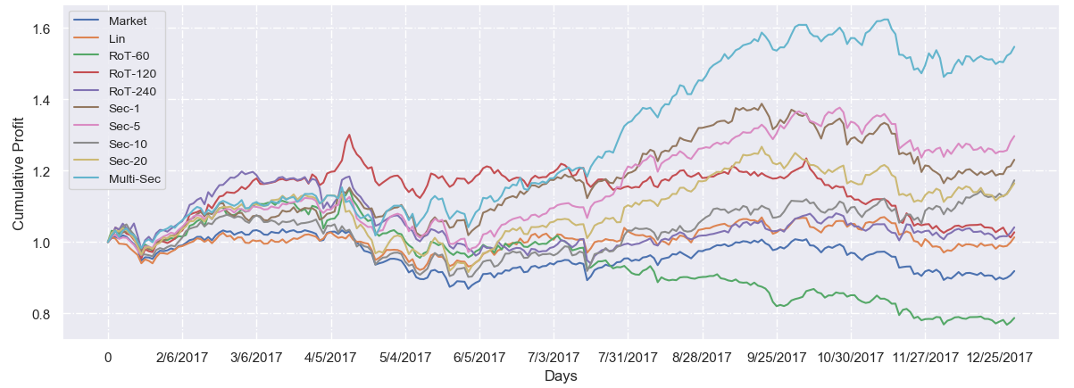
Figure 6: The cumulative profit curve of differnt methods with the portfolio of chossing top 50 stocks.

Figure  6 shows the cumulative profit curve for each method with $K$ as 50. As can be seen, our proposed second-order learning paradigm, $\mathrm{Sec}$ and $\mathrm{multi}$-$\mathrm{Sec}$, have the most profitable results over all baselines. In particular, $\mathrm{multi}$-$\mathrm{Sec}$ performs the best during a long period. Despite in the first half of 2017, rotation learning paradigm performs well and even achieve more profit than our algorithm, it loses a lot of money on the second half of 2017 due to the sudden distribution altering. In the second half of 2017, much more profit can be brought by $\mathrm{multi}$-$\mathrm{Sec}$, because $\mathrm{multi}$-$\mathrm{Sec}$ considers both short-term and long-term market states while $\mathrm{Sec}$ merely models single time scale. Furthermore, the performance of different time scale is alternating: $\mathrm{Sec}$-20 performs the best in March, while $\mathrm{Sec}$-5 generates the most profit after October. It indicates that the scale preference of the stock market is changing over time. In future work, we will consider to dynamically combine the multi-scale trends for more accurate prediction.

5 Related Work

In this section, we elaborate the related work for stock prediction in two parts: the first part is traditional methods including technical analysis and fundamental analysis, the second part is the machine learning techniques.

Technical analysis deals with the time-series historical market data, such as trading price and volume, and make predictions based on that. Due to the noisy nature of the stock market, technical analysts not only use raw price and volume data, but also explore many sorts of technical indicators Colby and Meyers (1988), which are mathematical transformations of price, volume and other inputs. One major limitation of the technical analysis is that it is incapable of unveiling the rules that govern the dynamics of the market beyond price data. Fundamental analysis Abarbanell and Bushee (1997), on the contrary, evaluates a stock in an attempt to assess its intrinsic value, by examining related economic, financial, and other qualitative and quantitative factors. Besides traditional technical/fundamental indicators, online information, such as news and forum, can also help people make better investment decision Nassirtoussi et al. (2015); Zhou et al. (2016).

Recently, machine learning techniques, which can automatically recognize the underlying patterns in the stock market with little human knowledge, have attracted many investors’ attention. Substantial researcher have already tried various models with multiple input indicators for stock prediction, such as linear regression Bermingham and Smeaton (2011); Mittal and Goel (2012); Izzah et al. (2017), decision tree Delen et al. (2013); Ballings et al. (2015) and neural networks Rather et al. (2015); Ding et al. (2015); Hafezi et al. (2015). Among existing machine learning techniques, the linear model has good interpretability, while non-linear models can capture the complex patterns. With the development of deep learning, many works use the Recurrent Neural networks (RNNs) for stock prediction because they can model strong temporal dynamics of the stock market. Recent work obtains more competitive performance on RNNs, for example, Nelson et.al built an LSTM network with a set of technical indicators as input to predict the stock trend Nelson et al. (2017). Zhang et.al proposed SFM Zhang et al. (2017) and applied it in the stock prediction task. Compared to LSTM, SFM decomposes the hidden states of memory cells into multiple frequency components, each of which models a particular frequency of latent trading patterns. The learned models by these machine learning methods characterize the underlying patterns of the stock market, and will be used in an arbitrary dataset constantly for future prediction.

No matter how complex existing models are, they are all designed based on the first-order i.d. assumption which assumes the stationary data distribution over time. However, due to the highly dynamic nature of the stock market, it is not adequate to predict the stock price on the strict first-order i.d. assumption.

6 Conclusion

In this paper, we address the dynamic and non-stationary property of the stock market, by introducing a second-order i.d. assumption. In contrast to existing methods that use the fixed model over time, we assume that the optimal prediction model is changing over time with certain patterns. Based on this assumption, we develop a second-order learning paradigm for capturing the second-order patterns. Furthermore, to presume more accurate prediction, the proposed model can capture the evolving second-order pattern with respect to both micro-scale and macro-scale. In the end, extensive experiments on real-world Chinese stock market data demonstrate that our approach can result in a significant improvement.

In the future, we will extend our work to other first-order models. Due to lacking the clear economic meaning, it will be more challenging to model the second-order evolving pattern of non-linear model. In addition, considering the alternating performance of the different scale method in back-testing, we plan to dynamically combine the multi-scale information for more profit.

References

- Abarbanell and Bushee [1997] Jeffrey S Abarbanell and Brian J Bushee. Fundamental analysis, future earnings, and stock prices. Journal of Accounting Research, 35(1):1–24, 1997.
- Ballings et al. [2015] Michel Ballings, Dirk Van den Poel, Nathalie Hespeels, and Ruben Gryp. Evaluating multiple classifiers for stock price direction prediction. Expert Systems with Applications, 42(20):7046–7056, 2015.
- Bermingham and Smeaton [2011] Adam Bermingham and Alan Smeaton. On using twitter to monitor political sentiment and predict election results. In Proceedings of the Workshop on Sentiment Analysis where AI meets Psychology (SAAIP 2011), pages 2–10, 2011.
- Brock et al. [1992] William Brock, Josef Lakonishok, and Blake LeBaron. Simple technical trading rules and the stochastic properties of stock returns. The Journal of finance, 47(5):1731–1764, 1992.
- Cervelló-Royo et al. [2015] Roberto Cervelló-Royo, Francisco Guijarro, and Karolina Michniuk. Stock market trading rule based on pattern recognition and technical analysis: Forecasting the djia index with intraday data. Expert systems with Applications, 42(14):5963–5975, 2015.
- Choe et al. [1993] Hyuk Choe, Ronald W Masulis, and Vikram Nanda. Common stock offerings across the business cycle: Theory and evidence. Journal of Empirical finance, 1(1):3–31, 1993.
- Colby and Meyers [1988] Robert W Colby and Thomas A Meyers. The encyclopedia of technical market indicators. Dow Jones-Irwin Homewood, IL, 1988.
- Delen et al. [2013] Dursun Delen, Cemil Kuzey, and Ali Uyar. Measuring firm performance using financial ratios: A decision tree approach. Expert Systems with Applications, 40(10):3970–3983, 2013.
- Ding et al. [2015] Xiao Ding, Yue Zhang, Ting Liu, and Junwen Duan. Deep learning for event-driven stock prediction. In Ijcai, pages 2327–2333, 2015.
- Fischer and Krauss [2018] Thomas Fischer and Christopher Krauss. Deep learning with long short-term memory networks for financial market predictions. European Journal of Operational Research, 270(2):654–669, 2018.
- Hafezi et al. [2015] Reza Hafezi, Jamal Shahrabi, and Esmaeil Hadavandi. A bat-neural network multi-agent system (bnnmas) for stock price prediction: Case study of dax stock price. Applied Soft Computing, 29:196–210, 2015.
- Hochreiter and Schmidhuber [1997] Sepp Hochreiter and Jürgen Schmidhuber. Long short-term memory. Neural computation, 9(8):1735–1780, 1997.
- Izzah et al. [2017] Abidatul Izzah, Yuita Arum Sari, Ratna Widyastuti, and Toga Aldila Cinderatama. Mobile app for stock prediction using improved multiple linear regression. In Sustainable Information Engineering and Technology (SIET), 2017 International Conference on, pages 150–154. IEEE, 2017.
- Kakushadze [2016] Zura Kakushadze. 101 formulaic alphas. Wilmott, 2016(84):72–81, 2016.
- Kamijo and Tanigawa [1990] Ken-ichi Kamijo and Tetsuji Tanigawa. Stock price pattern recognition-a recurrent neural network approach. In Neural Networks, 1990., 1990 IJCNN International Joint Conference on, pages 215–221. IEEE, 1990.
- Khaidem et al. [2016] Luckyson Khaidem, Snehanshu Saha, and Sudeepa Roy Dey. Predicting the direction of stock market prices using random forest. arXiv preprint arXiv:1605.00003, 2016.
- Lucas [1980] Robert E Lucas. Methods and problems in business cycle theory. Journal of Money, Credit and banking, 12(4):696–715, 1980.
- Lynch [2004] Merrill Lynch. The investment clock. Special report, 2004.
- Mittal and Goel [2012] Anshul Mittal and Arpit Goel. Stock prediction using twitter sentiment analysis. Standford University, CS229 (2011 http://cs229. stanford. edu/proj2011/GoelMittal-StockMarketPredictionUsingTwitterSentimentAnalysis. pdf), 15, 2012.
- Næs et al. [2011] Randi Næs, Johannes A Skjeltorp, and Bernt Arne Ødegaard. Stock market liquidity and the business cycle. The Journal of Finance, 66(1):139–176, 2011.
- Nassirtoussi et al. [2015] Arman Khadjeh Nassirtoussi, Saeed Aghabozorgi, Teh Ying Wah, and David Chek Ling Ngo. Text mining of news-headlines for forex market prediction: A multi-layer dimension reduction algorithm with semantics and sentiment. Expert Systems with Applications, 42(1):306–324, 2015.
- Nelson et al. [2017] David MQ Nelson, Adriano CM Pereira, and Renato A de Oliveira. Stock market’s price movement prediction with lstm neural networks. In Neural Networks (IJCNN), 2017 International Joint Conference on, pages 1419–1426. IEEE, 2017.
- Patel et al. [2015] Jigar Patel, Sahil Shah, Priyank Thakkar, and K Kotecha. Predicting stock market index using fusion of machine learning techniques. Expert Systems with Applications, 42(4):2162–2172, 2015.
- Preethi and Santhi [2012] G Preethi and B Santhi. Stock market forecasting techniques: A survey. Journal of Theoretical & Applied Information Technology, 46(1), 2012.
- Rather et al. [2015] Akhter Mohiuddin Rather, Arun Agarwal, and VN Sastry. Recurrent neural network and a hybrid model for prediction of stock returns. Expert Systems with Applications, 42(6):3234–3241, 2015.
- Savin et al. [2006] Gene Savin, Paul Weller, and Jānis Zvingelis. The predictive power of “head-and-shoulders” price patterns in the us stock market. Journal of Financial Econometrics, 5(2):243–265, 2006.
- Sharpe [1966] William F Sharpe. Mutual fund performance. The Journal of business, 39(1):119–138, 1966.
- Suh et al. [2004] Sang C Suh, Dan Li, and Jingmiao Gao. A novel chart pattern recognition approach: A case study on cup with handle. In Proc of Artificial Neural Network in Engineering Conf. Citeseer, 2004.
- Zhang et al. [2014] Xiangzhou Zhang, Yong Hu, Kang Xie, Shouyang Wang, EWT Ngai, and Mei Liu. A causal feature selection algorithm for stock prediction modeling. Neurocomputing, 142:48–59, 2014.
- Zhang et al. [2017] Liheng Zhang, Charu Aggarwal, and Guo-Jun Qi. Stock price prediction via discovering multi-frequency trading patterns. In Proceedings of the 23rd ACM SIGKDD International Conference on Knowledge Discovery and Data Mining, pages 2141–2149. ACM, 2017.
- Zhou et al. [2016] Zhenkun Zhou, Jichang Zhao, and Ke Xu. Can online emotions predict the stock market in china? In International Conference on Web Information Systems Engineering, pages 328–342. Springer, 2016.