Scalable Quantitative Verification For Deep Neural Networks

Abstract

Despite the functional success of deep neural networks (DNNs), their trustworthiness remains a crucial open challenge. To address this challenge, both testing and verification techniques have been proposed. But these existing techniques provide either scalability to large networks or formal guarantees, not both. In this paper, we propose a scalable quantitative verification framework for deep neural networks, i.e., a test-driven approach that comes with formal guarantees that a desired probabilistic property is satisfied. Our technique performs enough tests until soundness of a formal probabilistic property can be proven. It can be used to certify properties of both deterministic and randomized DNNs. We implement our approach in a tool called provero and apply it in the context of certifying adversarial robustness of DNNs. In this context, we first show a new attack-agnostic measure of robustness which offers an alternative to purely attack-based methodology of evaluating robustness being reported today. Second, provero provides certificates of robustness for large DNNs, where existing state-of-the-art verification tools fail to produce conclusive results. Our work paves the way forward for verifying properties of distributions captured by real-world deep neural networks, with provable guarantees, even where testers only have black-box access to the neural network.

I Introduction

The past few years have witnessed an increasing adoption of deep neural networks (DNNs) in domains such as autonomous vehicles [5, 52, 35], drones [24] or robotics [16, 67], where mispredictions can have serious long-term consequences. Robustness, privacy, and fairness have emerged as central concerns to be addressed for safe adoption of DNNs [9, 47, 33, 43, 51, 1, 37]. Consequently, there has been a growing attention to testing and verification of neural networks for properties of interest.

To establish that the resulting DNNs have the desired properties, a large body of prior work has focused on techniques based on empirical testing [56, 53, 65, 19] or specialized attack vectors [36, 59, 42, 2, 47, 20]. While such techniques are useful, they do not rigorously quantify how sure we can be that the desired property is true after testing.

In contrast to testing approaches, formal verification seeks to provide rigorous guarantees of correctness. Inspired by the success of model checking in the context of hardware and software verification, the earliest formal verification methodologies in the context of deep neural networks focused on qualitative verification, i.e., whether a system satisfies a given specification. Prior work in this category has been following the model checking paradigm wherein a given DNN is encoded as a model using constraints grounded in a chosen theory. Then a satisfiability solver (often modulo the chosen theory) is invoked to check if there exists an execution of the system that violates the given specification [44, 14, 39, 26].

The proposed techniques in this category appear to have three limitations. Firstly, they require white-box access to the models and specialized procedures to transform the DNNs to a specification, limiting their generality. Secondly, the performance of the underlying feasibility solver degrades severely with the usage of non-linear constraints, leading to analyses that do not scale to larger models. Thirdly, prior techniques are limited to deterministic neural networks, while extensive research effort has been invested in designing randomized DNNs, especially to enhance robustness [12, 33, 11].

Such qualitative verification considers only two scenarios: either a DNN satisfies the property, or it does not. However, neural networks are stochastically trained, and more importantly, they may run on inputs drawn from an unknown distribution at inference time. Properties of interest are thus often probabilistic and defined over an input distribution (e.g., fairness [37] or robustness to distributional changes [1]). Hence, qualitative verification is unsuitable for such properties.

An alternative approach is to check how often a property is satisfied by a given DNN under a given input distribution. More specifically, one can assert that a DNN satisfies a property $\psi$ with a desirably high probability $1-\delta$. Unlike ad-hoc testing, quantitative verification [3] aims to provide soundness, i.e., when it confirms that $\psi$ is true with probability $p$, then the claim can be rigorously deduced from the laws of probability. For many practical applications, knowing that the chance of failure is controllably small suffices for deployment. For instance, it has been suggested that road safety standards for self-driving cars specify sufficiently low failure rates of the perceptual sub-systems, against which implementations can be verified [28, 25, 55]. Further, we show the role of quantitative verification in the specific context of adversarial robustness (see Section II-A).

In this paper, we present a new quantitative verification algorithm for DNNs called provero, tackling the following problem: Given a logical property $\psi$ specified over a space of inputs and outputs of a DNN and a numerical threshold $\theta$, decide whether $\psi$ is true for less than $\theta$ fraction of the inputs. provero is a procedure that achieves the above goal with proven soundness: When it halts with a ‘Yes’ or ‘No’ decision, it is correct with probability $1-\delta$ and within approximation error $\eta$ to the given $\theta$. The verifier can control the desired parameters $(\eta,\delta)$, making them arbitrarily close to zero. That is, the verifier can have controllably high certainty about the verifier’s output, and $\theta$ can be arbitrarily precise (or close to the ground truth). The lower the choice of $(\eta,\delta)$ used by the verifier, the higher is the running time.

provero is based on sampling, and it makes only one assumption—the ability to take independent samples from the space over which $\psi$ is defined. This makes the verification procedure considerably general and stand-alone. The verifier only needs black-box access to the DNN, freeing it up from assuming anything about the internal implementation of the DNNs. The DNN can be deterministic or from a general family of non-deterministic DNNs. This allows checking probabilistic properties of deterministic DNNs and of randomization procedures defined over DNNs.

Our paper makes the following contributions:

• We present a new quantitative verification algorithm for neural networks. The framework is fairly general: It assumes only black-box access to the model being verified, and assumes only the ability to sample from the input distribution over which the property is asserted.

• We implement our approach in a tool called provero that embodies sound algorithms and scales quantitative verification for adversarial robustness to large real-world DNNs, both deterministic and randomized, within $1$ hour.

• In the context of certifying adversarial robustness, our empirical evaluation presents a new attack-agnostic measure of robustness and shows that provero can produce certificates with high confidence on instances where existing state-of-the-art qualitative verification does not provide conclusive results.

II Application: Adversarial Robustness

For concreteness, we apply our approach to verifying the robustness of neural networks. In proving robustness, the analyst has to provide a space of inputs over which the robustness holds. Often, this space is defined by all inputs that are within a perturbation bound $\epsilon$ of a given input $\mathbf{x}$ in the $L_{p}$ norm [17]. Different distance norms have been used such as $L_{0}$, $L_{1}$, $L_{2}$ and $L_{\infty}$. The $L_{p}$ norm is defined as $\left\lVert\mathbf{x}-\mathbf{x}^{\prime}\right\rVert_{p}=(|x^{\prime}_{1}-x_{1}|^{p}+|x^{\prime}_{2}-x_{2}|^{p}+\ldots+|x^{\prime}_{n}-x_{n}|^{p})^{1/p}$. A neural network $f$ is defined to be robust with respect to a given input $\mathbf{x}$ if $\forall\mathbf{x}^{\prime}$ such that $\left\lVert\mathbf{x}-\mathbf{x}^{\prime}\right\rVert_{p}<\epsilon,$ we have $f(\mathbf{x})=f(\mathbf{x}^{\prime})$.

For a given neural network $f$ and input point $\mathbf{x}$, there always exists some perturbation size beyond which there are one or more adversarial samples. We refer to this minimum perturbation with non-zero adversarial examples as $\epsilon_{min}$, which is the ground truth the security analyst wants to know. Attack procedures are best-effort methods which find upper bounds for $\epsilon_{min}$ but cannot provably show that these bounds are tight [58, 8, 2]. Verification procedures aim to prove the absence of adversarial examples below a given bound, i.e., they can establish lower bounds for $\epsilon_{min}$. We call such verified lower bounds $\epsilon_{verf}$. Most verifiers proposed to date for robustness checking are qualitative, i.e., given a perturbation size $\epsilon_{verf}$, they output whether adversarial examples are absent within $\epsilon_{verf}$. If the verification procedure is sound and outputs ‘Yes’, then it is guaranteed that there are no adversarial examples within $\epsilon_{verf}$, i.e., the robustness property is satisfied. When the verifier says ‘No’, if the verifier is complete, then it is guaranteed that there are indeed adversarial examples within $\epsilon_{verf}$. If the verifier is incomplete and prints ‘No’, the result is inconclusive.

Let us introduce a simple quantitative measure of robustness called the adversarial density. Adversarial density is the fraction of inputs around a given input $\mathbf{x}$ which are adversarial examples. We explain why adversarial density is a practically useful quantity and much easier to compute for large DNNs than $\epsilon_{min}$. We can compute perturbation bounds below which the adversarial density is non-zero but negligibly small, and we empirically show these bounds are highly correlated with estimates of $\epsilon_{min}$ obtained by state-of-the-art attack methods.

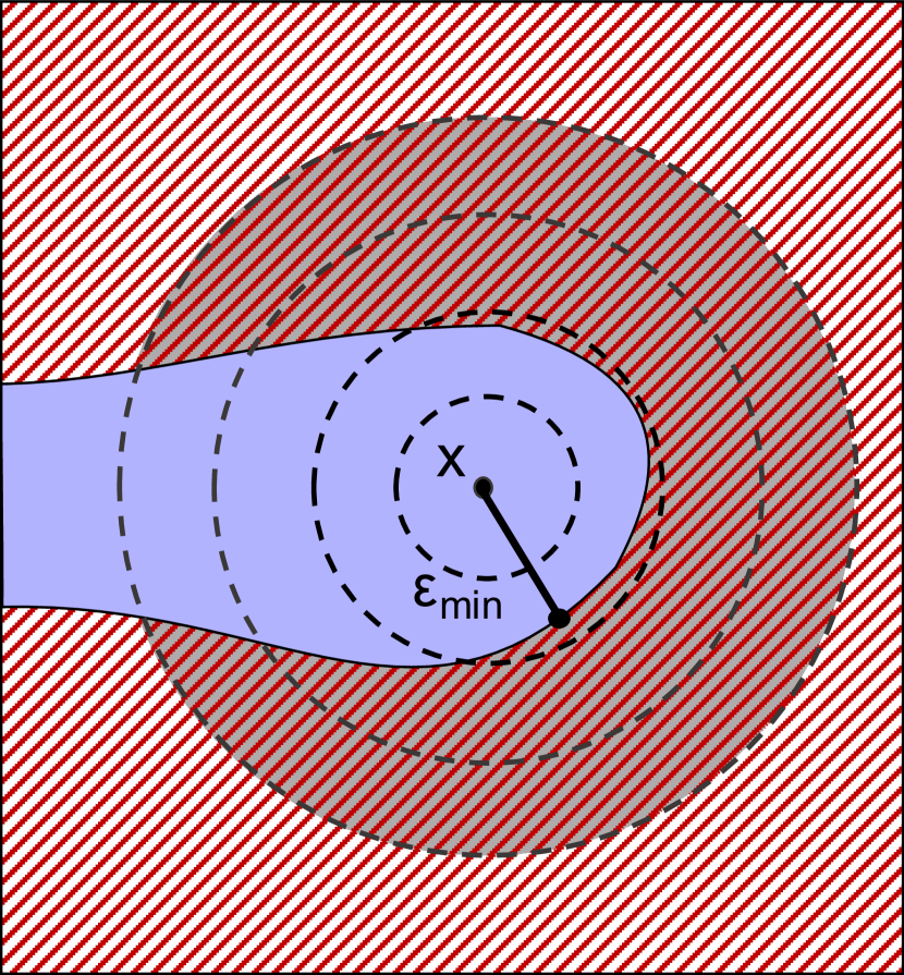
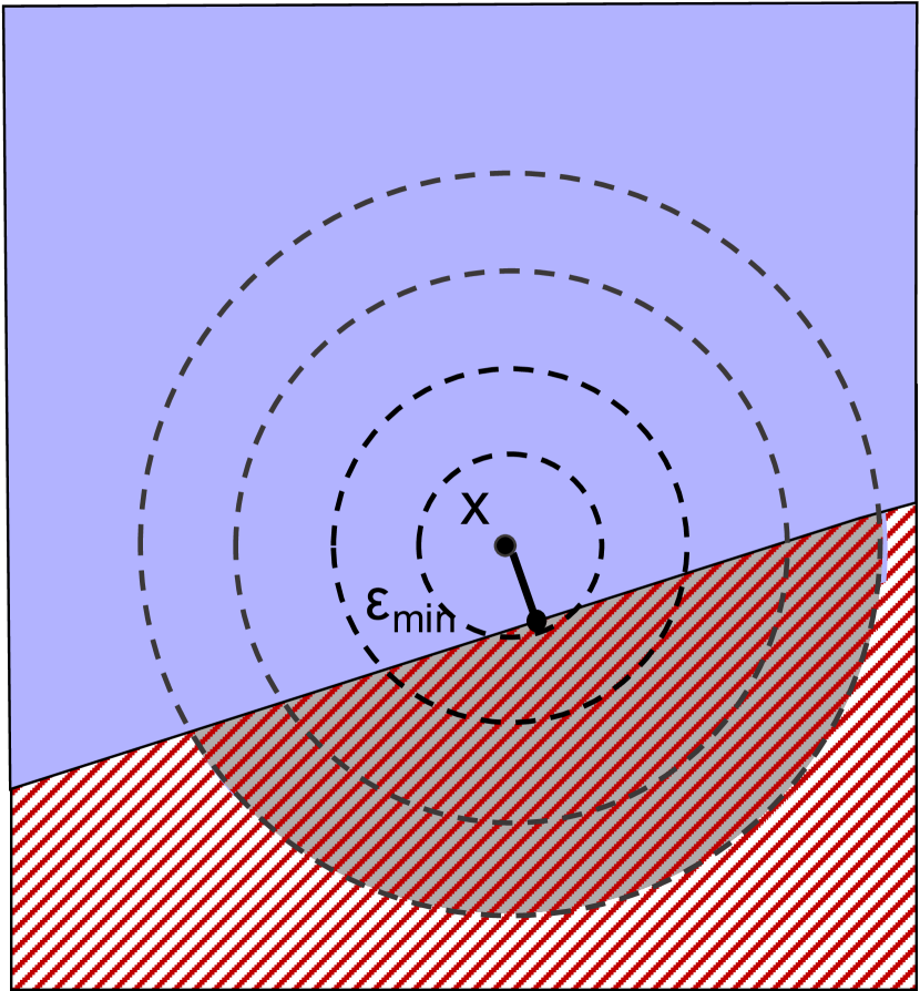
Figure 1: The decision boundaries of two binary classifiers $f_{1}$ (left) and $f_{2}$ (right) around an input $\mathbf{x}$ are shown. The correct classification region for $\mathbf{x}$ is shown in purple (solid), while the incorrect classification region is shown in red (hashed). The concentric circles show the equidistant points from $\mathbf{x}$ in $L_{2}$-norm drawn up to a bound $\epsilon$. The classifier $f_{1}$ has a better (larger) minimum perturbation than $f_{2}$, but has a worse (larger) adversarial density because a majority of points within $\epsilon$ distance of $\mathbf{x}$ are in the incorrect classification region. Therefore, the smoothened version of $f_{2}$ will classify $\mathbf{x}$ correctly, while the smoothened $f_{1}$ will not. Picking the base classifier with the better adversarial density, rather than minimum perturbation, will lead to better accuracy in a smoothening defense.

II-A Minimum Perturbation vs. Density

It is reasonable to ask why adversarial density is relevant at all for security analysis. After all, the adversary would exploit the weakest link, so the minimum perturbation size $\epsilon_{min}$ is perhaps the only quantity of interest. We present concrete instances where adversarial density is relevant.

First, we point to randomized smoothing as a defense technique, which has provable guarantees of adversarial robustness [33, 12, 11, 64]. The defense uses a “smoothed” classifier $g$ that averages the behavior of a given neural net $f$ (called the base classifier) around a given input $\mathbf{x}$. More specifically, given a base classifier $f$, the procedure samples perturbations of $\mathbf{x}$ within $\epsilon$ from a specific noise distribution and outputs the most likely class $c$ such that $argmax_{c\in\mathcal{Y}}Pr[f(\mathbf{x}+\epsilon)=c]$. Notice that this procedure computes the probability of $f$ returning class $c$—typically by counting how often $f$ predicts class $c$ over many samples—rather than considering the ”worst-case” example around $\mathbf{x}$. Said another way, these approaches estimate the adversarial density for each output class under some input distribution. Therefore, when selecting between two base classifiers during training, we should pick the one with the smallest adversarial density for the correct class, irrespective of their minimum adversarial perturbation size.

To illustrate this point, in Figure 1 we show two DNNs $f_{1}$ and $f_{2}$, as potential candidates for the base classifier in a randomized smoothing procedure. Notice that $f_{1}$ has a better (larger) $\epsilon_{min}$ than $f_{2}$. However, more of the inputs within the $\epsilon$-ball of the input $\mathbf{x}$ (inside the red hashed circle) are classified as the wrong label by $f_{1}$ in comparison to $f_{2}$. Thus, a smoothed classifier with $f_{1}$ as a base classifier would misclassify $\mathbf{x}$ where the smoothed classifier with base $f_{2}$ would classify correctly. This explains why we should choose the classifier with the smaller adversarial density rather than one based on the minimum perturbation because the smoothing process is not susceptible to worst-case examples by its very construction. This motivates why computing adversarial density is useful for adversarial robustness defenses.

Second, we point out that estimating minimal perturbation bounds has been a difficult problem. Attack procedures, which provide an upper bound for $\epsilon_{min}$, are constantly evolving. This makes robustness evaluations attack-specific and a moving target. On the other hand, qualitative verification techniques can certify that the DNN has no adversarial examples below a certain perturbation, which is a lower bound on the adversarial perturbation [26, 57, 48, 13]. However, these analyses do not scale well with deep networks and can lead either to timeouts or inconclusive results for large real-world DNNs. Furthermore, they are white-box, requiring access to the model internals and work only for deterministic neural networks. We show in this work that verifying adversarial density bounds is easy to compute even for large DNNs. We describe procedures that require only black-box access, the ability to sample from desired distributions and hence are attack-agnostic.

In particular, we show an empirical attack-agnostic metric for estimating robustness of a given DNN and input $\mathbf{x}$ called adversarial hardness. It is highest perturbation bound for which the adversarial density is below a suitably low $\theta$. We can search empirically for the highest perturbation bound $\epsilon_{\texttt{Hard}}$, called the adversarial hardness, for which a sound quantitative certifier says ‘Yes’ when queried with $(f,\mathbf{x},$$\epsilon_{\texttt{Hard}}$$,\theta,\delta,\eta)$—implying that $f$ has suitably low density of adversarial examples for perturbation bounds below $\epsilon_{\texttt{Hard}}$.

Adversarial hardness is a measure of the difficulty of finding an adversarial example by uniform sampling. Surprisingly, we find that this measure strongly correlates with perturbation bounds produced by prominent white-box attacks (see Section VII). Given this strong correlation, we can effectively use adversarial hardness as a proxy for perturbation sizes obtained from specific attacks, when comparing the relative robustness of two DNNs.

We caution readers that adversarial hardness is a quantitative measure and technically different from $\epsilon_{min}$, the distance to the nearest adversarial example around $\mathbf{x}$. But both these measures provide complementary information about the concentration of adversarial examples near a perturbation size.

III Problem Definition

We are given a neural network and a space of its inputs over which we want to assert a desirable property $\psi$ of the outputs of the network. Our framework allows one to check whether $\psi$ is true for some specified ratio $\theta$ of all possible values in the specified space of inputs. For instance, one can check whether most inputs, a sufficiently small number of inputs, or any other specified constant ratio of the inputs satisfies $\psi$. The specified ratio parameter $\theta$ is called a threshold.

Formally, let $\psi(\mathcal{I},f,\Phi)\in\{0,1\}$ be a property function over a neural network $f$, a subset of all possible inputs to the neural network $\mathcal{I}$ and user-specified parameters $\Phi$. We assume that we can efficiently draw samples from any probability distribution over $\mathcal{I}$ that the analyst desires. For a given distribution $D$ over $\mathcal{I}$, let $p_{D}=\mathbf{E}_{x\sim D}[\psi(x,f,\Phi)]$. $p_{D}$ can be viewed as the probability that $\psi$ evaluates to $1$ for $x$ sampled from $\mathcal{I}$ according to $D$. When clear from context, we omit $D$ and simply use $p$ to refer to $p_{D}$.

Ideally, one would like to design an algorithm that returns ‘Yes’ if $p\leq\theta$ and ’No’ otherwise. Such exact quantification is intractable, so we are instead interested in an algorithm $\mathcal{A}$ that returns ‘Yes’ if $p\leq\theta$ and ’No’ otherwise, with two controllable approximation parameters $(\eta,\delta)$. The procedure should be theoretically sound, ensuring that when it produces ‘Yes’ or ‘No’ results, it is correct with probability at least $1-\delta$ within an additive bound on its error $\eta$ from the specified threshold $\theta$. Specifically, we say that algorithm $\mathcal{A}$ is sound if:

$$Pr[\mathcal{A}(\psi,\theta,\eta,\delta)~{}\text{returns {`Yes'}}~{}|~{}p\leq\theta]\geq 1-\delta$$

$$Pr[\mathcal{A}(\psi,\theta,\eta,\delta)~{}\text{returns {`No'}}~{}|~{}p>\theta+\eta]\geq 1-\delta$$

The analyst has arbitrary control over the confidence $\delta$ about $\mathcal{A}$’s output correctness and the precision $\eta$ around the threshold. These values can be made arbitrarily small approaching zero, increasing the runtime of $\mathcal{A}$. The soundness guarantee is useful—it rigorously estimates how many inputs in $\mathcal{I}$ satisfy $\psi$, serving as a quantitative metric of satisfiability.

The presented framework makes very few assumptions. It can work with any specification of $\mathcal{I}$, as long as there is an interface to be able to sample from it (as per any desired distribution) efficiently. The neural network $f$ can be any deterministic function. In fact, it can be any “stateless” randomized procedure, i.e., the function evaluated on a particular input does not use outputs produced from prior inputs. This general class of neural networks includes, for instance, Bayesian neural networks [22] and many other ensembles of neural network architectures [4]. The framework permits specifying all properties of fairness, privacy, and robustness highlighted in recent prior work [3, 40], for a much broader class of DNNs.

Our goal is to present sound and scalable algorithms for quantitative verification, specifically targeting empirical performance for quantitatively certifying robustness of DNNs. The framework assumes black-box access to $f$, which can be deterministic or non-deterministic. Our techniques can directly check qualitative certificates produced from randomized robustness-enhancing defenses, one example of which is the recent work called PixelDP [33] (see Section VII-C).

IV Approach Overview

IV-A Sampling

Given a property $\psi$ over a sampleable input space $\mathcal{I}$ and a neural network $f$, our approach works by sampling $N$ times independently from $\mathcal{I}$. We test $f$ on each sample as input. Let $X_{i}$ be a 0-1 random variable denoting the result of the trial with sample $i$, where $X_{i}=1$ if the $\psi(x,f,\Phi)$ is true and $X_{i}=0$ otherwise. Let $X$ be the random variable denoting the number of trials in $X_{1},X_{2},\dots,X_{N}$ for which the property is true. Then, the standard Chernoff bounds (see [38]) given below form the main workhorse underlying our algorithms:

Lemma IV.1

Given independent 0-1 random variables $X_{1},\ldots,X_{N}$, let $X=\sum_{i=1}^{N}{X_{i}}$, $\mu=\frac{\mathbf{E}[X]}{N}$, and $\hat{p}=\frac{X}{N}$. For $0<\eta<1$:

$$Pr[\hat{p}\geq\mu+\eta]\leq e^{\frac{-N\eta^{2}}{3\mu}}$$

$$Pr[\hat{p}\leq\mu-\eta]\leq e^{\frac{-N\eta^{2}}{2\mu}}$$

Note that the probability $p$ we are interested in bounding in our quantitative verification framework is exactly $\mu$ in Lemma IV.1. More specifically, the probability depends on the neural network and distribution over the inputs, $p=\mathbf{E}_{x\sim D}[\psi(x,f,\Phi)]$, where $D$ is a distribution over $\mathcal{I}$. Using a framework based on sampling and Chernoff bounds admits considerable generality. The only assumption in applying the Lemma IV.1 is that all samples are independent. If the neural network does not compute information during one trial (or execution under one sample) and use it in another trial, as is the case for all neural networks we study, trials will be independent. For any deterministic neural network, all samples are drawn independently and identically distributed in $\mathcal{I}$, so Chernoff bounds are applicable. For randomized DNNs, we can think of the $i^{th}$ trial as evaluating a potentially different neural network (sampled from some distribution of functions) on the given sample. Here, the output random variables may not be identically distributed due to the randomization used by the neural network itself. However, Lemma IV.1 can still be used even for non-identically distributed trials but independent.

We discuss an estimation-based strategy that applies Chernoff bounds in a straight-forward manner next. Such a solution has high sample complexity for quantitative verification of adversarial robustness. We then propose hypothesis-based solutions which are sound and have much better empirical sample complexity for real-world DNNs. Our proposed algorithms still rely only on Chernoff-style bounds, but are carefully designed to internally vary parameters (on which Chernoff bounds are invoked) to reduce the number of samples needed to dispatch the asserted property.

IV-B An Estimation-based Solution

One way to quantitatively verify a property through sampling is to directly apply Chernoff bounds to the empirical estimate of the mean $\hat{p}$ in $N$ trials. The solution is to take $N>\frac{12\cdot ln\frac{1}{\delta}}{\eta^{2}}$ samples, and decide ‘Yes’ if $\hat{p}\leq\theta+\frac{\eta}{2}$ and ‘No’ if $\hat{p}>\theta+\frac{\eta}{2}$. This is a common estimation approach, for instance used in the prediction step in the certified defense mechanism PixelDP [33]. By Lemma IV.1, one can show that $\hat{p}$ is within $\pm\frac{\eta}{2}$ additive error of $p$ with confidence higher than $1-\delta$. Therefore, the procedure is sound since $Pr[p\not\in[\hat{p}-\frac{\eta}{2},\hat{p}+\frac{\eta}{2})]\leq\delta$ by Lemma IV.1, for all $0\leq p\leq 1$.

In this solution, the number of samples increase quadratically with decreasing $\eta$. For example, if the $\theta=0.1,\eta=10^{-3},\delta=0.01$, directly applying Chernoff bounds will require over $55\times 10^{6}$ samples. Even for an optimized architecture such as BranchyNet [54] that reports $70.9$ ms on average inference time per sample for a ResNet ($152$ layers) the estimation approach would take more than $1083$ GPU compute hours. This is a prohibitive cost. For randomized DNNs, which internally compute expectations, the runtime of the estimation baseline approach can be even larger. For example, the randomization used in PixelDP can have $3-42\times$ inference overhead compared to deterministic DNNs [33].

Our work provides new algorithms that utilize much fewer samples on average. In the example of BranchyNet mentioned above, if the true probability $p$ is $0.3$, our approach requires $4246$ samples to return a ‘No’ answer with confidence greater than $0.99$. The main issue with the estimation algorithm is that it does not utilize the knowledge of the given $\theta$ in deciding the number of samples it needs.

IV-C Our Approach

The number of samples needed for Chernoff bounds depend on how far is the true probability $p$ that we are trying to bound from the given threshold $\theta$. Intuitively, if $p$ and $\theta$ are far apart in the interval $[0,1]$, then a small number of samples are sufficient to conclude with high certainty that $p\leq\theta$ or $p>\theta+\eta$ (for small $\eta$). The estimation approach takes the same number of samples irrespective of how far $p$ and $\theta$ are. Our algorithms terminate quickly by checking for “quick-to-test” hypothesis early, yielding the sample complexity comparable to the estimation only in the worst case.

We propose new algorithms, the key idea of which is to use cheaper (in sample complexity) hypothesis tests to decide ‘Yes’ or ‘No’ early. Given the threshold $\theta$ and the error $\eta$, the high-level idea is to propose alternative hypotheses on the left side of $\theta$ and on the right side of $\theta+\eta$. We choose the hypotheses and a sampling procedure such that if any of the hypotheses on the left side of $\theta$ are true, then we can return ‘Yes’. Similarly, if any of the hypotheses on the right side of $\theta+\eta$ are true, then we can return ‘No’. Thus, we can potentially return much faster when the true probability $p$ is further from the threshold $\theta$.

Algorithm 1 Metaprovero ($\theta,\eta,\delta$)

1:while cond do

2:     pick $\theta_{1}<\theta_{2}\leq\theta$

3:     ans = Tester ($\theta_{1},\theta_{2},\delta$)

4:     if ans == ‘Yes’ then return ‘Yes’      

5:     pick $\theta_{2}>\theta_{1}\geq\theta+\eta$

6:     ans = Tester ($\theta_{1},\theta_{2},\delta$)

7:     if ans == ‘No’ then return ‘No’      

8:return Tester ($\theta,\theta+\eta,\delta$)

Algorithm 2 Tester ($\theta_{1},\theta_{2},\delta$)

1:$N=\frac{(\sqrt{3\theta_{1}}+\sqrt{2\theta_{2}})^{2}}{(\theta_{2}-\theta_{1})^{2}}ln\frac{1}{\delta}$

2:$\eta_{1}=(\theta_{2}-\theta_{1})\Big{(}1+\sqrt{\frac{2}{3}\frac{\theta_{2}}{\theta_{1}}}\Big{)}^{-1}$

3:$\eta_{2}=\theta_{2}-\theta_{1}-\eta_{1}$

4:sample $N$ times

5:$\hat{p}=\frac{1}{N}\sum_{i=1}^{N}{X_{i}}$ $\triangleright$ $X_{i}$ - samples that satisfy the property

6:if $\hat{p}\leq\theta_{1}+\eta_{1}$ then return ‘Yes’

7:if $\hat{p}>\theta_{2}-\eta_{2}$ then return ‘No’

8:return None

The overall meta-level structure of our algorithms is simple and follows Algorithm 1, called Metaprovero. In lines 2 and 5, we pick the alternative hypotheses on the left and right of the given threshold $\theta$ respectively. We sample a certain number of samples, estimate the ratio $\hat{p}$ (by invoking Tester in lines 3 and 6), and check if we can prove that conditions involving the alternative intermediate thresholds ($\theta_{1}$ and $\theta_{2}$) are satisfied with the desired input parameters $(\eta,\delta)$ using Chernoff bounds. If the check succeeds, the algorithm can return ‘Yes’ or ‘No’; otherwise, the process repeats until a condition which guarantees soundness is met.

The internal thresholds are picked so as to soundly prove or refute that $p$ lies in certain ranges in $[0,1]$. This is done by testing certain intervals $p$ is (or is not) in. For instance, Metaprovero tests a pair of hypotheses $p\leq\theta_{1}$ and $p>\theta_{2}$ simultaneously (line 3). Notice that for the intervals on the left side of $\theta$ ($\theta_{1}<\theta_{2}\leq\theta$, chosen in line 2 in Alg. 1), the call to Tester can result in proving that $p\leq\theta_{1}$ with desired confidence $\delta$ and error tolerance $\eta$. In this case, since $\theta_{1}<\theta$, we will have proven the original hypothesis $p\leq\theta$ and the algorithm can return ‘Yes’ soundly. We call such intervals, which are to the left of $\theta$, as proving intervals. Conversely, refuting intervals are on the right side of $\theta+\eta$. The choice of $\theta_{1}$ and $\theta_{2}$ on line 5 in Alg. 1 is such that they are larger than $\theta+\eta$. When we can prove that $p>\theta_{2}$, i.e., the Tester call on line 6 returns ‘No’, then we can soundly return ‘No’ because $\theta_{2}>\theta+\eta$ implies $p>\theta+\eta$.

Figure 2: Example run of Metaprovero ($0.1,10^{-3},0.01$) given that $p=0.3$. On the left-hand side, Metaprovero cannot prove that $p\leq\theta$ since $p$ is greater than left-side $\theta_{2_{l}}$. Next, Metaprovero chooses the refuting interval on the right-hand side. Since $p>\theta_{2_{r}}$, Tester returns ‘No’ and Metaprovero can prove that $p>\theta+\eta$.

In Fig. 2, we consider an example run of Metaprovero given that the true probability $p=0.3$ (highlighted in blue) and the input parameters are $\theta=0.1,\eta=10^{-3},\delta=0.01$. Metaprovero picks the proving interval $(\theta_{1l},\theta_{2l})=(0.03,0.06)$ on the left of $\theta$ and calls Tester which returns ‘No’. This means that the true probability is greater than $\theta_{1l}$ with high confidence. Metaprovero then picks an interval $(\theta_{1r},\theta_{2r})=(0.15,0.25)$ on the right-side of $\theta+\eta$. Here Tester returns with confidence higher than $1-\delta$ that $p>\theta_{2r}$. Since $\theta_{2r}>\theta+\eta$ we can conclude that the true probability is greater than $\theta$ with error $\eta$.

The key building block of this algorithm is the Tester sub-procedure (Algorithm 2), which employs sampling to check hypotheses. Informally, the Tester does the following: Given two intermediate thresholds, $\theta_{1}$ and $\theta_{2}$, if the true probability $p$ is either smaller than $\theta_{1}$ or greater than $\theta_{2}$, it returns ‘Yes’ or ‘No’ respectively with high confidence. If $p\in(\theta_{1},\theta_{2})$ then the tester does not have any guarantees. Notice that a single invocation of the Tester checks two hypotheses simultaneously, using one set of samples. The number of samples needed are proven sufficient in Section V-B.

One can directly invoke Tester with $\theta_{1}=\theta$ and $\theta_{2}=\theta+\eta$ but that might lead to a very large number of samples, $\mathcal{O}(1/\eta^{2})$. Thus, the key challenge is to judiciously call the Tester on hypotheses with smaller sample complexity such that we can refute or prove faster in most cases. To this end, notice that Metaprovero leaves out two algorithmic design choices: stopping conditions and the strategy for choosing the proving and refuting hypotheses (highlighted in Alg. 1). We propose and analyze an adaptive binary-search-style algorithm where we change our hypotheses based on the outcomes of our sampling tests (Section V-A). We show that our proposed algorithm using this strategy is sound. When $p$ is extremely close to $\theta$, these algorithms are no worse than estimating the probability, requiring roughly the same number of samples.

V Algorithms

We provide an adaptive algorithm for quantitative certification that narrows the size of the intervals in the proof search, similar to a binary-search strategy (Section V-A). This algorithm build on the base of the Tester primitive which we explain in Section V-B.

V-A The BinPCertify Algorithm

We propose an algorithm BinPCertify (Algorithm 3) where instead of fixing the intervals beforehand we narrow our search by halving the intervals. The user-specified input parameters for BinPCertify are the threshold $\theta$, the error bound $\eta$ and the confidence parameter $\delta$. The interval creation strategy is off-loaded to the CreateInterval procedure outlined in Algorithm 4. The interval size $\alpha$ is initially set to the largest possible as Tester would require less samples on wider intervals (Algorithm 4, lines 1-3). Then, the BinPCertify algorithm calls internally the procedure CreateInterval to create proving intervals (on the left side of $\theta$, Alg. 3, line 6) and refuting intervals (on the right side of $\theta+\eta$, Alg. 3, line 10). Note that for the refuting intervals, we keep the left-side fixed, $\theta_{1}=\theta+\eta$ and for the proving intervals we keep the right-side fixed, i.e., $\theta_{2}=\theta$ . For each iteration of BinPCertify, the strategy we use is to halve the intervals by moving the outermost thresholds closer to $\theta$ (Alg. 4, lines 5-7). For these intermediate hypotheses, Tester checks if it can prove or disprove the assert $p\leq\theta$ (lines 8 and 12). It continues to do so alternating the proving and refuting hypotheses until the size of both intervals becomes smaller than the error bound $\eta$ (line 14). If only on one side of the threshold CreateInterval returns intervals with size $\alpha>\eta$, BinPCertify checks those hypotheses. If the size of the proving and refuting intervals returned by CreateInterval is $\eta$, then the final check is directly invoked on $(\theta,\theta+\eta)$ and returned to the user (line 15).

The algorithm BinPCertify returns ‘Yes’ or ‘No’ with soundness guarantees as defined in Section III. We give our main theorem here and defer the proof to Section VI:

Theorem V.1

For an unknown value $p\in[0,1]$, a given threshold $\theta\in[0,1],\eta\in(0,1),\delta\in(0,1]$, BinPCertify returns a ‘Yes’ or ‘No’ with the following guarantees:

$$Pr[\text{{BinPCertify} returns {`Yes'}}~{}|~{}p\leq\theta]\geq 1-\delta$$

$$Pr[\text{{BinPCertify} returns {`No'}}~{}|~{}p>\theta+\eta]\geq 1-\delta$$

Algorithm 3 BinPCertify $(\theta,\eta,\delta)$

1:$\theta_{1_{l}}=\theta_{{2}_{l}}=0$

2:$\theta_{1_{r}}=\theta_{{2}_{r}}=0$

3:$n=3+max(0,log(\frac{\theta}{\eta}))+max(0,log(\frac{1-\theta-\eta}{\eta}))$

4:$\delta_{min}=\delta/n$ $\triangleright$ minimum confidence per call to Tester

5:while True do

6:     $\theta_{1_{l}},\theta_{{2}_{l}}$ = CreateInterval($\theta,\theta_{1_{l}},\theta_{{2}_{l}},\eta$, True)

7:     if $\theta_{{2}_{l}}-\theta_{1_{l}}>\eta$ then

8:         ans = Tester($\theta_{1_{l}},\theta_{2_{l}}$, $\delta_{min}$)

9:         if ans == ‘Yes’ then return ‘Yes’               

10:     $\theta_{1_{r}},\theta_{{2}_{r}}$ = CreateInterval($\theta,\theta_{1_{r}},\theta_{{2}_{r}},\eta,$ False)

11:     if $\theta_{{2}_{r}}-\theta_{1_{r}}>\eta$ then

12:         ans = Tester($\theta_{1_{r}},\theta_{2_{r}}$, $\delta_{min}$)

13:         if ans == ‘No’ then return ‘No’               

14:     if $\theta_{{2}_{r}}-\theta_{1_{r}}\leq\eta$ and $\theta_{{2}_{l}}-\theta_{1_{l}}\leq\eta$ then

15:         return Tester($\theta,\theta+\eta$, $\delta_{min}$)      

Algorithm 4 CreateInterval ($\theta,\theta_{1},\theta_{2},\eta$, left)

1:if $\theta==0$ and left then return $(\theta,\theta+\eta)$

2:if $\theta_{1}==0$ and $\theta_{2}==0$ and left then: return ($0,\theta$)

3:if $\theta_{1}==0$ and $\theta_{2}==0$ and $\neg$left then: return ($\theta+\eta,1$)

4:$\alpha=\theta_{2}-\theta_{1}$

5:if left then

6:     return ($\theta_{2}$ - max($\eta,\alpha/2$), $\theta_{2}$)

7:return ($\theta_{1},\theta_{1}$ + max($\eta,\alpha/2$))

V-B Tester Primitive

The tester takes as input two thresholds $\theta_{1},\theta_{2}$ such that $\theta_{1}<\theta_{2}$ and confidence parameter $\delta$ and returns ‘Yes’ when $p\leq\theta_{1}$ with confidence higher than $1-\delta$ and ‘No’ when $p>\theta_{2}$ with confidence higher than $1-\delta$. If $p\in(\theta_{1},\theta_{2}]$ the Tester returns without guarantees.

The procedure for implementing the Tester is simple. Following the procedure outlined in Algorithm 2, we take $N=\frac{(\sqrt{3\theta_{1}}+\sqrt{2\theta_{2}})^{2}}{(\theta_{2}-\theta_{1})^{2}}ln\frac{1}{\delta}$ number of independent samples and estimate the ratio of these 0-1 trials as $\hat{p}$. The Tester returns ‘Yes’ if $\hat{p}\leq\theta_{1}+\eta_{1}$ and ‘No’ if $\hat{p}>\theta_{2}-\eta_{2}$ where $\eta_{1}$ and $\eta_{2}$ are error parameters (lines 2 and 3). If $\theta_{1}+\eta_{1}<\hat{p}<\theta_{2}-\eta_{2}$, our implementation returns ’None’. The following lemma establishes the soundness of the tester, and follows directly from applying Chernoff bounds on $\hat{p}$.

Lemma V.2

Given the thresholds ($\theta_{1},\theta_{2}$) and confidence parameter $\delta$, Tester has following soundness guarantees:

$$Pr[\text{{Tester} returns `Yes'}~{}|~{}p\leq\theta_{1}]\geq 1-\delta$$

$$Pr[\text{{Tester} returns `No'}~{}|~{}p>\theta_{2}]\geq 1-\delta$$

Proof:

The proof follows directly the Chernoff bounds. ∎

Figure 3: Tester considers the boundary $t=\theta_{1}+\eta_{1}=\theta_{2}-\eta_{2}$ that allows to distinguish $p\leq\theta_{1}$ or $p>\theta_{2}$.

Using the estimated probability $\hat{p}$, Tester returns ‘Yes’ if $\hat{p}\leq\theta_{1}+\eta_{1}$ and ‘No’ if $\hat{p}\geq\theta_{2}-\eta_{2}$ with probability greater than $1-\delta$. Otherwise, it returns ‘None’. We want to choose values $\eta_{1},\eta_{2}\in(0,1)$ such that $Pr[\hat{p}\geq\theta_{1}+\eta_{1}~{}|~{}p\leq\theta_{1}]\leq\delta$ and $Pr[\hat{p}\leq\theta_{2}-\eta_{2}~{}|~{}p>\theta_{2}]\leq\delta$.

To derive the minimum number of samples for the estimated $\hat{p}$, the key idea is to use one set of samples to check two hypotheses, $p\leq\theta_{1}$ and $p>\theta_{2}$, simultaneously. To do so, we find a point $t\in(\theta_{1},\theta_{2})$ which serves as a decision boundary for the estimate probability $\hat{p}$. We illustrate this in Figure 3: it shows $(t,\eta_{1},\eta_{2})$ and the two probability distributions for $\hat{p}$ given $p=\theta_{1}$ and $p=\theta_{2}$, respectively. The distributions for the case $p<\theta_{1}$ will be shifted further to the left, and the case $p>\theta_{2}$ will be shifted further to the right; so these are extremal distributions to consider. It can be seen that $t$ is chosen such that $Pr[\hat{p}>t|p\leq\theta_{1}]$ as well as $Pr[\hat{p}<t|p>\theta_{2}]$ are bounded (shaded red) by probability $\delta$. Using the additive Chernoff bounds (Lemma IV.1), for a given $\theta_{1}$ and $\theta_{2}$, the number of samples $N$ is the maximum of $3\theta_{1}\frac{1}{\eta_{1}^{2}}ln\frac{1}{\delta}$ and $2\theta_{2}\frac{1}{\eta_{2}^{2}}ln\frac{1}{\delta}$.

Taking the maximum ensures that the probabilities of the both the hypotheses, $p<\theta_{1}$ and $p>\theta_{2}$, are being simultaneously upper bounded. We leave the detail analysis for the supplementary material.

VI Soundness

In this section, we prove that our proposed algorithm satisfies soundness as defined in Section III. BinPCertify uses the Tester primitive on certain intervals in sequence. Depending on the strategy, the size of the intervals and the order of testing them differs. But, the algorithm terminates immediately if the Tester returns ‘Yes’ on a proving interval or ‘No’ on a refuting one. The meta-algorithm captures this structure on line 2-5 and BinPCertify algorithm instantiates this general structure. When none of these optimistic calls to Tester are successful, the algorithm makes a call to the Tester on the remaining interval in the worst case. Given the same basic structure of algorithms as per the meta-algorithm Metaprovero, we now prove the following key theorem:

Lemma VI.1

Let $E$ be the event that the algorithm $\cal{A}\in\{\textsc{BinPCertify}\}$ fails, then $Pr[E]\leq\delta$.

Proof:

Fix any input to $\cal{A}$, and consider the execution of $\cal{A}$ under those inputs. Without loss of generality, we can order the intervals tested by $\cal{A}$ in the sequence that $\cal{A}$ invokes the Tester on them in that execution. Let the sequence of intervals be numbered from $1,\ldots,i$, for some value $i$.

Now, let us bound the probability of the event $E_{i}$, which is when $\cal{A}$ tests intervals $1,\ldots,i$ and fails. To do so, we consider events associated with each invocation of Tester $j\in[1,i]$. Let $R_{j}$ be the event that $\cal{A}$ returns immediately after invoking the Tester on the $j$-th interval. Let $C_{j}$ denote the event that Tester returns a correct answer for the $j$-th interval. If $E_{i}$ is true, then $\cal{A}$ terminates immediately after testing the $i$-th interval and fails. This event happens only if two conditions are met: First, $\cal{A}$ did not return immediately after testing intervals $1,\ldots,i-1$; and second, $\cal{A}$ returns a wrong answer at $i$-th interval and does terminate. Therefore, we can conclude that the event $E_{i}=\bar{C}_{i}\cap R_{i}\cap\bar{R}_{i-1}\cap\ldots\cap\bar{R}_{1}$. The probability of failure $Pr[E_{i}]$ for each event $E_{i}$ is upper bounded by $Pr[\bar{C}_{i}]$.

Lastly, let $E$ be the total failure probability of $\cal{A}$. We can now use a union bound over possible failure events $E_{1},\ldots,E_{n}$, where $n$ is the maximum number of intervals $\cal{A}$ can possibly test under any given input. Specifically:

$$Pr[E]=Pr[E_{1}\cup E_{2}\ldots\cup E_{n}]\leq\sum_{i=1}^{n}Pr[E_{i}]\leq\sum_{i=1}^{n}Pr[\bar{C}_{i}]$$

By analyzing $\sum_{i=1}^{n}Pr[\bar{C}_{i}]$ in the context of our specific algorithm BinPCertify, we show that the quantity is bounded by $\delta$ (Lemma VI.2). ∎

Lemma VI.2

Under any given input ($\theta,\eta,\delta$), let $C_{i}$ be the event that $i$-th call made by BinPCertify to the Tester is correct and let $n$ be the total number of calls to Tester by BinPCertify. Then, $\sum_{i=1}^{n}Pr[\bar{C}_{i}]\leq\delta$.

Proof:

We can upper bound the number of proving intervals on the left by $n_{l}\leq 1+log\frac{\theta}{\eta}$. Similarly, for the right side of $\theta+\eta$, number of refuting intervals is $n_{r}\leq 1+log\frac{1-\theta-\eta}{\eta}$. Lastly, there is only $1$ call to the Tester on the interval $\eta$ (line $19$, Alg. 3). The total number of intervals tested in any one execution of BinPCertify is at most $n=3+log\frac{\theta}{\eta}+log\frac{1-\theta-\eta}{\eta}$. Each call to the Tester is done with confidence parameter $\delta_{min}=\frac{\delta}{n}$, therefore by Lemma V.2, the failure probability of any call is at most $\frac{\delta}{n}$. It follows that the $Pr[\bar{C}_{i}]\leq n\cdot\frac{\delta}{n}=\delta$

∎

VII Evaluation

• Scalability: For a given timeout, what is the largest model that provero and existing qualitative analysis tools can produce conclusive results.

• Utility in attack evaluations: How does adversarial hardness computed with provero compare with the efficacy of state-of-the-art attacks?

• Applicability to randomized models: Can provero certify properties of randomized DNNs?

• Performance. How many samples are needed by our new algorithms vis-a-vis the estimation approach (Section IV-B)?

We implement our algorithms in a prototype tool called provero and evaluate the robustness of $38$ deterministic neural networks trained on $2$ datasets: MNIST [32] and ImageNet [46]. For MNIST, we evaluate on 100 images from the model’s respective test set. In the case of ImageNet, we pick from the validation set as we require the correct label. Table I provides the size statistics of these models. In addition, we evaluate the randomized model publicly provided by PixelDP [33], which has a qualitative certificate of robustness.

TABLE I: Neural network architectures used in our evaluation.

Dataset	Arch	Description	#Hidden Units
MNIST(BM1)	FFNN	6-layer feed-forward	3010
	convSmall	2-layer convolutional	3604
	convMed	3-layer convolutional	4804
	convBig	6-layer convolutional	34688
	convSuper	6-layer convolutional	88500
	skip	residual	71650
ImageNet (BM2)	VGG16	16-layer convolutional	15,086,080
	VGG19	19-layer convolutional	16,390,656
	ResNet50	50-layer residual	36,968,684
	Inception_v3	42-layer convolutional	32,285,184
	DenseNet121	121-layer convolutional	49,775,084

ERAN Benchmark (BM1)

Our first benchmark consists of $33$ moderate size neural networks trained on the MNIST dataset. These are selected to aid a comparison with a state-of-the-art qualitative verification framework called ERAN [48]. We selected all the models which ERAN reported on. These models range from 2-layer neural networks to 6-layer neural networks with up to about $90K$ hidden units. We use the images used to evaluate the ERAN tool.

Larger Models (BM2)

The second benchmark consists of $5$ larger deep-learning models pretrained on ImageNet: VGG16, VGG19, ResNet50, InceptionV3 and DenseNet121. These models were obtained via the Keras framework with Tensorflow backend. These have about $15-50M$ hidden units.

All experiments were run on GPU (Tesla V100-SXM2-16GB) with a timeout of $600$ seconds per image for the MNIST, $2000$ seconds for ImageNet models, and $3600$ seconds for the randomized PixelDP model.

VII-A Utility in Attack Evaluation

provero can be used to directly certify if the security analyst has a threshold they want to check, for example, obtained from an external specification. Another way to understand its utility is by relating the quantitative bounds obtained from provero with those reported by specific attacks. When comparing the relative robustness of DNNs to adversarial attacks, a common evaluation methodology today is to find the minimum adversarial perturbation with which state-of-the-art attacks can produce at least one successful adversarial example. If the best known attacks perform worse on one DNN versus another, on a sufficiently many test inputs, then the that DNN is considered more robust.

TABLE II: Attack correlation for the PGD and C&W attack for the models in BM1 and BM2 using Pearson’s coefficient ($\rho$). For all, statistical significance $p<0.01$.

Models	$\rho$ (PGD)	$\rho$ (C&W)
convBigRELU__DiffAI	0.9617	0.7509
convMedGRELU__PGDK_w_0.1	0.8143	0.6686
convMedGRELU__PGDK_w_0.3	0.7699	0.6715
convMedGRELU__Point	0.8461	0.982
convMedGSIGMOID__PGDK_w_0.1	0.8533	0.8903
convMedGSIGMOID__PGDK_w_0.3	0.9394	0.913
convMedGSIGMOID__Point	0.9424	0.9605
convMedGTANH__PGDK_w_0.1	0.9521	0.9334
convMedGTANH__PGDK_w_0.3	0.9567	0.8718
convMedGTANH__Point	0.7592	0.9817
convSmallRELU__DiffAI	0.9504	0.5127
convSmallRELU__PGDK	0.7803	0.6411
convSmallRELU__Point	0.893	0.9816
convSuperRELU__DiffAI	0.687	0.3856
DenseNet-res	0.7168	0.4879
ffnnRELU__PGDK_w_0.1_6_500	0.8932	0.9577
ffnnRELU__PGDK_w_0.3_6_500	0.7039	0.6496
ffnnRELU__Point_6_500	0.954	0.9788
ffnnSIGMOID__PGDK_w_0.1_6_500	0.8706	0.8955
ffnnSIGMOID__PGDK_w_0.3_6_500	0.9402	0.9201
ffnnSIGMOID__Point_6_500	0.8906	0.9489
ffnnTANH__PGDK_w_0.1_6_500	0.8156	0.9508
ffnnTANH__PGDK_w_0.3_6_500	0.9104	0.9485
ffnnTANH__Point_6_500	0.8998	0.8435
mnist_conv_maxpool	0.9664	0.9699
mnist_relu_3_100	0.9668	0.9448
mnist_relu_3_50	0.9702	0.9298
mnist_relu_4_1024	0.8945	0.9723
mnist_relu_5_100	0.7472	0.9629
mnist_relu_6_100	0.9845	0.9868
mnist_relu_6_200	0.9699	0.9412
mnist_relu_9_100	0.979	0.9725
mnist_relu_9_200	0.8165	0.9652
ResNet50	0.7929	0.6932
skip__DiffAI	0.7344	0.6298
VGG16	0.8064	0.8297
VGG19	0.7224	0.7335
Inception-v3	0.5806	0.4866

provero offers a new capability: we can measure the ratio of adversarial samples within a specified perturbation bound of a given test input $\mathbf{x}$ (see Section II). Specifically, we can compute the adversarial density by uniformly sampling in the $L_{p}$ ball of $\mathbf{x}$, and checking if the ratio of adversarial samples is very small (below $\theta=10^{-3}$). By repeating this process for different perturbations bounds, we empirically determine the adversarial hardness (or $\epsilon_{\texttt{Hard}}$)—the largest perturbation bound below which provero certifies the adversarial density to be that small (returns ‘Yes’) and above which provero does not (returns ‘No’). We use density threshold $\theta=10^{-3}$, error tolerance $\eta=10^{-3}$, and confidence parameter $\delta=0.01$.

provero computes the adversarial hardness with black-box access. As a comparison point, we evaluate against two white-box attacks — PGD [36] for $L_{\infty}$ and C&W [9] for $L_{2}$ implemented in CleverHans [41] (v3.0.1) — $2$ prominent attacks that are recommended for the $L_{p}$ norms we consider [7]. White-box attacks enable the attacker complete access to internals; therefore, they are more powerful than black-box attacks today. Both PGD and C&W are gradient-based adversarial attacks. For PGD, we perform $30$ attacks on different values of $\epsilon$ to identify the minimum value that an adversarial input can be identified. For C&W, we identify the best $\epsilon$ it is able to identify for a given amount of resource (iterations).

Our main empirical result in this experiment is that $\epsilon_{\texttt{Hard}}$ is strongly correlated with $\epsilon_{min}$. Figure 4 and Figure 5 show the correlation visually for two models: it shows that the perturbation bounds found by these two separate attacks are different, but both correlate with the adversarial hardness of the certification instance produced by provero. The Pearson correlation for all models is reported in Table II for all cases where the compared white-box attacks are successful The average Pearson correlation between the perturbation found by PGD, $\epsilon_{PGD}$, and $\epsilon_{\texttt{Hard}}$ over all models is $0.858$ and between the perturbation found by C&W, $\epsilon_{C\&W}$, and $\epsilon_{\texttt{Hard}}$ is $0.8438$. We take $25$ images per model to calculate the correlation. The significance level is high (p-value is below $0.01$ for all cases).

Recall that provero is sound, so the estimate of adversarial hardness $\epsilon_{\texttt{Hard}}$ is close to the ground truth with high probability ($99\%$). This metric is an attack-agnostic metric, computed by uniform sampling and without white-box access to the model. The strong correlation shows that PGD and C&W attacks find smaller $\epsilon_{min}$ for easier certification instances, and larger $\epsilon_{min}$ for harder instances. This suggests that when comparing the robustness of two models, one can consider adversarial hardness as a useful attack-agnostic metric, complementing evaluation on specific attacks.

Figure 4: Correlation graph between $L_{\infty}$ bounds provided by provero and PGD for a fully connected feedforward with sigmoid (FFNN) on MNIST.

Figure 5: Correlation graph between $L_{2}$ bounds provided by provero and C&W for a fully connected feedforward (FFNN) with sigmoid on MNIST.

Figure 6: provero and ERAN verified robustness per perturbation size for BM1 for threshold $\theta=0.0001$, error $\eta=0.001$ and confidence $\delta=0.01$.

VII-B Scalability

We test provero on $38$ models, which range from $3K-50M$ hidden units. We select $100$ input images for each model and retain all those inputs for which the model correctly classifies. We tested $11$ perturbation size ($L_{\infty}$) from $0.01$ to $0.25$ for BM1 and $4$ perturbation size ($L_{2}$) from ${2/255}$ to $14/255$ for BM2. This results in a total of $36971$ test images for $38$ models. We run each test image with provero with the following parameters: $(\theta=0.0001,\eta=0.001$ and $\theta=0.01,\eta=0.01,\delta=0.01)$ (for BM1) $(\theta=0.001,\eta=0.001$ and $\theta=0.01,\eta=0.01,\delta=0.01)$ (for BM2). We find that provero scales producing answers within the timeout of $600$ seconds for BM1 and $2000$ seconds for BM2 per test image. Less than $2\%$ input cases for BM2 and less than $5\%$ for BM1 return ’None’, i.e., provero cannot certify conclusively that there are less or more than than the queried thresholds. For all other cases, provero provides a ‘Yes’ or ‘No’ results.

As a comparison point, we tried to compare with prior work on quantitative verification [3], prototyped in a tool called NPAQ. While NPAQ provides direct estimates rather than the ‘Yes’ or ‘No’ answers provero produces, we found that NPAQ supports only a sub-class of neural networks (BNNs) and of much smaller size. Hence, it cannot support or scale for any of the models in our benchmarks, BM1 and BM2.

Secondly, we tested ERAN which is considered as the most scalable qualitative verification tool. ERAN initially was not able to parse these models. After direct correspondence with the authors of ERAN, the authors added support for requisite input model formats. After applying these changes, we confirmed that the current implementation of ERAN time out on all the BM2 models. provero finishes on these within a timeout of $2000$ seconds.

We successfully run ERAN on BM1, which are smaller benchmarks that ERAN reported on. There are total of $4$ analyses in ERAN. We evaluate on the DeepZono and DeepPoly domains but for the DeepPoly, on our evaluation platform, ERAN runs out of memory and could not analyze the neural networks in BM1. The remaining analyses, RefineZono and RefinePoly are known to achieve or improve the precision of the DeepZono or DeepPoly domain at the cost of larger running time by calling a mixed-integer programming solver [50]. Hence, we compare with the most scalable of these $4$ analyses, namely the DeepZono domain.

Figure 6 plots the precision of ERAN against provero for all $11$ perturbation sizes. We find that for a perturbation size of more than $0.05$, ERAN’s results are inconclusive, i.e., the analysis reports neither ‘Yes’ nor ‘No’ for more than $50\%$ of the inputs, likely due to imprecision in over-approximations of the analysis. Figure 6 shows that the verified models reduces for higher perturbations $\epsilon$. This is consistent with the findings in the ERAN paper: ERAN either takes longer or is more imprecise for non-robust models and higher $\epsilon$ values [50]. In all cases where ERAN is inconclusive, provero successfully finishes within the $600$ second timeout for all $35431$ test images and values of $\epsilon$. In above $95\%$ of these cases, provero produces high-confidence ‘Yes’ or ‘No’ results.

As a sanity check, on cases where ERAN conclusively outputs a ‘Yes’, provero also reports ‘Yes’. With comparable running time, provero is able to obtain quantitative bounds for all perturbation sizes. From these experimental results, we conclude provero is a complementary analysis tool that can be used to quantitatively certify larger models and for larger perturbation sizes, for which our evaluated qualitative verification framework (ERAN) is inconclusive. To the best of our knowledge, this is the first work to give any kind of sound quantitative guarantees for such large models.

VII-C Applicability to Randomized DNNs

So far in our evaluation we have focused on deterministic DNNs, however, provero can certify the robustness of randomized DNNs. To demonstrate this generality, we take a model obtained by a training procedure called PixelDP that adds differentially private noise to make the neural network more robust. The inference phase of a PixelDP network uses randomization: instead of picking the label with the maximum probability, it samples from the noise layer and calculates an expectation of the output value. PixelDP also produces a certified perturbation bound for which it guarantees the model to be robust for a given input image. Note that qualitative verification tools such as ERAN require white-box access and work with deterministic models, so they would not be able to verify the robustness of randomized PixelDP DNNs.

We contacted the authors to obtain the models used in PixelDP [33]. The authors pointed us to the PixelDP ResNet28-10 model trained on CIFAR10 as the main representative of the technique. We randomly select $25$ images in the CIFAR10 dataset and for each image we obtain the certified perturbation bound $\epsilon_{pixeldp}$ produced by PixelDP itself. We configure PixelDP to internally estimate $\epsilon_{pixeldp}$ using $25$ samples from the noise layer as recommended in their paper. This bound, $\epsilon_{PixelDP}$, is the maximum bound for which PixelDP claims there are no adversarial samples within the $L_{2}$ ball.

We use provero to check the certificate $\epsilon_{PixelDP}$ produced by PixelDP, using the following parameters $\theta=0.01,\eta=0.01,\delta=0.01$. provero reports ‘Yes’, implying that the model has adversarial density under these bounds. Under the same threshold $\theta=10^{-2},\eta=10^{-2}$ we tested for larger perturbation sizes: from $\epsilon=0.1$ to $0.25$.

Our findings in this experiment are that provero can certify low adversarial density for perturbation bounds much larger than the qualitative certificates produced by PixelDP. In particular, provero certifies that for $\epsilon=5\times\epsilon_{PixelDP}$, the PixelDP model has less than $10^{-2}$ adversarial examples with confidence at least $99\%$. provero offers complimentary quantitative estimates of robustness for PixelDP.

VII-D Performance

Our estimation solution outlined in Section IV-B applies Chernoff bounds directly. For a given precision parameter $\eta$, it requires a large number of samples, within a factor of $1/\eta^{2}$. While we do not escape from this worst case, we show that our proposed algorithms improve over the estimation baseline empirically. To this end, we record the number of samples taken for each test image and compare it to the number of samples as computed for the estimation approach.

We find that provero requires $27\times$ less samples than the estimation approach for values of $\eta=0.01,\theta=0.01$ and $687\times$ less samples for values of $\eta=0.001,\theta=0.0001$ for BM1. For larger models in BM2 and values of $\eta=0.001,\theta=0.001$, provero requires $74\times$ less samples than the estimation solution and $\eta=0.01,\theta=0.01$.

In our implementation, we use a batch-mode to do the inference for models in BM1 and BM2, speeding up the running time of the sampling process by a factor of $3\times$. This leads to average times of $29.78$ seconds per image for BM1 for a batch size of $128$. For the models in BM2 we used different batch sizes so we report the average time per sample as $0.003$ seconds which can be used to derive the running time based. For ($\theta=0.0001,\eta=0.001$) and all values of $\epsilon$, the average number of samples over all images is $80,424$ (median value is $83,121$, standard deviation is $14,303$). For VGG16 the average number of samples is around $657,885$, for VGG19 it is around $644,737$ and for InceptionV3 $664,397$ samples, respectively, for $\theta=0.001,\eta=0.001$. For both $\theta=0.01,\eta=0.01$ and $\theta=0.001,\eta=0.001$, for VGG16 the average number of samples is $737,297$, for VGG19 it is $722,979$ and for InceptionV3 $744,792$ average number of samples, resulting in about $74\times$ less samples than the estimation approach.

For the PixelDP model, provero takes $20,753$ samples. Since PixelDP models internally take $25$ samples from the noise layer, the time taken for inference on one given input itself is higher. provero reports an average running time per test image of roughly $1,500$ seconds.

VIII Related Work

Qualitative verification methodologies have sought to exploit the advances in combinatorial solving, thereby consisting of satisfiability modulo theories (SMT) solvers-based approaches [23, 26, 27, 14, 39] or integer linear programming approaches [57, 34, 10]. Despite singficiant progress over the years, the combinatorial solving-based approaches do not scale to deep neural networks.

Consequently, techniques to address scalability often sacrifice completeness: abstract interpretation-based techniques [15, 48, 50, 49] are among the most scalable verification procedures that over-approximate the activation functions with abstract domains. Similarly, optimization-based approaches [64, 45, 13] produce a certificate of robustness for a given input: a lower bound on the minimum perturbation bound $\epsilon_{min}$ such that there are no adversarial examples within that a $\epsilon_{min}$ ball. These techniques are, however, incomplete and catered to only ReLU activations [64] and fully-connected layers [68, 18].

A promising line of incomplete techniques has been proposed employing two complementary techniques: Lipschitz computation and linear approximations. Hein and Andriushchenko [21] propose an analytical analysis based on the Lipschitz constant, but the approach assumes that a differentiable activation function (thus excluding ReLU activations) and can handle only two layers. Boopathy et al [6], Weng et al. [62], Zhang et al [68] have further improved the scalability of these techniques but they are still limited to $80,000$ hidden units. While the lower and upper bounds are sound, their tightness is not guaranteed. In another line of work, Weng et al. [63] employ extreme value theory to estimate a lower bound on $\epsilon_{min}$ albeit without theoretical guarantees of the soundness of the obtained bounds. provero differs fundamentally from classical verification approaches in our focus on the development of a quantitative verification framework with rigorous guarantees on computed estimates.

Baluta et al. [3] propose a quantitative framework that outputs estimates of how often a property holds. network into a logical formula and use model counting tools. Their approach, however, is instantiated to a specific type of neural networks, namely binarized neural networks, and its scalability is limited to networks with around $50,000$ parameters. In contrast, provero scales to DNNs with millions of parameters while preserving the formal guarantees of the white-box approach. Webb et al. [61] proposed a Monte Carlo-based approach for rare events to estimate the ratio of adversarial examples. In this work, we take a property testing approach wherein we ask if the proportion of inputs that violate a property is less than a given threshold (in which case we say yes) or it is $\eta$-far from the threshold (in which case we say no). While both approaches are black-box and rely on sampling, provero returns a yes or no answer with user-specified high confidence, whereas the statistical approach proposed by Webb et al. does not provide such guarantees. A related area is statistical model checking [31, 29, 30] that relies on sampling schemes [60] to accept a given hypothesis. provero algorithm is similar to a sequential sampling plan [66] but provero’s insight is that each test checks “cheaper” hypotheses in a binary-search manner. In particular, in case of provero, we design hypothesis in a manner that more expensive hypothesis tests are delayed as much as possible.

IX Conclusion

provero introduces an algorithm for verifying quantitative properties of neural networks, assuming only black-box access, and with much better test sample complexity than compared baselines. Our algorithm offers, in particular, a powerful new attack-agnostic way of evaluating adversarial robustness for deep neural networks.

References

- [1] D. Amodei, C. Olah, J. Steinhardt, P. Christiano, J. Schulman, and D. Mané, “Concrete problems in ai safety,” arXiv preprint arXiv:1606.06565, 2016.
- [2] A. Athalye, N. Carlini, and D. Wagner, “Obfuscated gradients give a false sense of security: Circumventing defenses to adversarial examples,” in ICML’18, 2018.
- [3] T. Baluta, S. Shen, S. Shine, K. S. Meel, and P. Saxena, “Quantitative verification of neural networks and its security applications,” in CCS’19, 2019.
- [4] D. Barber and C. M. Bishop, “Ensemble learning in bayesian neural networks,” Nato ASI Series F Computer and Systems Sciences, vol. 168, pp. 215–238, 1998.
- [5] M. Bojarski, D. Del Testa, D. Dworakowski, B. Firner, B. Flepp, P. Goyal, L. D. Jackel, M. Monfort, U. Muller, J. Zhang, and Others, “End to end learning for self-driving cars,” arXiv, 2016.
- [6] A. Boopathy, T.-W. Weng, P.-Y. Chen, S. Liu, and L. Daniel, “Cnn-cert: An efficient framework for certifying robustness of convolutional neural networks,” in AAAI’19, 2019.
- [7] N. Carlini, A. Athalye, N. Papernot, W. Brendel, J. Rauber, D. Tsipras, I. Goodfellow, and A. Madry, “On evaluating adversarial robustness,” arXiv preprint arXiv:1902.06705, 2019.
- [8] N. Carlini, P. Mishra, T. Vaidya, Y. Zhang, M. Sherr, C. Shields, D. Wagner, and W. Zhou, “Hidden voice commands.” in USENIX’16, 2016.
- [9] N. Carlini and D. Wagner, “Towards evaluating the robustness of neural networks,” in SP’17, 2017.
- [10] C.-H. Cheng, G. Nührenberg, and H. Ruess, “Maximum resilience of artificial neural networks,” in ATVA’17, 2017.
- [11] J. M. Cohen, E. Rosenfeld, and J. Z. Kolter, “Certified adversarial robustness via randomized smoothing,” arXiv preprint arXiv:1902.02918, 2019.
- [12] G. S. Dhillon, K. Azizzadenesheli, Z. C. Lipton, J. Bernstein, J. Kossaifi, A. Khanna, and A. Anandkumar, “Stochastic activation pruning for robust adversarial defense,” arXiv preprint arXiv:1803.01442, 2018.
- [13] K. Dvijotham, R. Stanforth, S. Gowal, T. Mann, and P. Kohli, “A Dual Approach to Scalable Verification of Deep Networks,” in UAI’18, 2018.
- [14] R. Ehlers, “Formal verification of piece-wise linear feed-forward neural networks,” in ATVA’17, 2017.
- [15] T. Gehr, M. Mirman, D. Drachsler-Cohen, P. Tsankov, S. Chaudhuri, and M. Vechev, “Ai2: Safety and robustness certification of neural networks with abstract interpretation,” in SP’18, 2018.
- [16] A. Giusti, J. Guzzi, D. C. Ciresan, F.-L. He, J. P. Rodriguez, F. Fontana, M. Faessler, C. Forster, J. Schmidhuber, G. D. Caro, D. Scaramuzza, and L. M. Gambardella, “A Machine Learning Approach to Visual Perception of Forest Trails for Mobile Robots,” IEEE Robotics and Automation Letters, 2016.
- [17] I. J. Goodfellow, J. Shlens, and C. Szegedy, “Explaining and harnessing adversarial examples,” arXiv preprint arXiv:1412.6572, 2014.
- [18] D. Gopinath, H. Converse, C. Pasareanu, and A. Taly, “Property inference for deep neural networks,” in ASE’19. IEEE, 2019, pp. 797–809.
- [19] D. Gopinath, G. Katz, C. S. Păsăreanu, and C. Barrett, “Deepsafe: A data-driven approach for assessing robustness of neural networks,” in ATVA’18, 2018.
- [20] D. Gopinath, C. S. Pasareanu, K. Wang, M. Zhang, and S. Khurshid, “Symbolic execution for attribution and attack synthesis in neural networks,” in ICSE’19, 2019.
- [21] M. Hein and M. Andriushchenko, “Formal guarantees on the robustness of a classifier against adversarial manipulation,” in NIPS’17, 2017.
- [22] R. Houthooft, X. Chen, Y. Duan, J. Schulman, F. De Turck, and P. Abbeel, “Curiosity-driven exploration in deep reinforcement learning via bayesian neural networks,” arXiv preprint arXiv:1605.09674, 2016.
- [23] X. Huang, M. Kwiatkowska, S. Wang, and M. Wu, “Safety verification of deep neural networks,” in CAV’17, 2017.
- [24] K. D. Julian, J. Lopez, J. S. Brush, M. P. Owen, and M. J. Kochenderfer, “Policy compression for aircraft collision avoidance systems,” in DASC’16, 2016.
- [25] N. Kalra and S. M. Paddock, “Driving to safety: How many miles of driving would it take to demonstrate autonomous vehicle reliability?” Transportation Research Part A: Policy and Practice, vol. 94, 2016.
- [26] G. Katz, C. Barrett, D. L. Dill, K. Julian, and M. J. Kochenderfer, “Reluplex: An efficient smt solver for verifying deep neural networks,” in CAV’17, 2017.
- [27] G. Katz, D. A. Huang, D. Ibeling, K. Julian, C. Lazarus, R. Lim, P. Shah, S. Thakoor, H. Wu, A. Zeljić et al., “The marabou framework for verification and analysis of deep neural networks,” in CAV’19, 2019.
- [28] P. Koopman and B. Osyk, “Safety argument considerations for public road testing of autonomous vehicles,” SAE Technical Paper, Tech. Rep., 2019.
- [29] M. Kwiatkowska, G. Norman, and D. Parker, “Stochastic model checking,” in International School on Formal Methods for the Design of Computer, Communication and Software Systems, 2007, pp. 220–270.
- [30] ——, “Prism: probabilistic model checking for performance and reliability analysis,” ACM SIGMETRICS Performance Evaluation Review, vol. 36, no. 4, pp. 40–45, 2009.
- [31] K. G. Larsen and A. Legay, “Statistical model checking past, present, and future,” in International Symposium On Leveraging Applications of Formal Methods, Verification and Validation. Springer, 2014, pp. 135–142.
- [32] Y. LeCun and C. Cortes, “MNIST handwritten digit database,” 2010.
- [33] M. Lecuyer, V. Atlidakis, R. Geambasu, D. Hsu, and S. Jana, “Certified robustness to adversarial examples with differential privacy,” arXiv preprint arXiv:1802.03471, 2018.
- [34] W. Lin, Z. Yang, X. Chen, Q. Zhao, X. Li, Z. Liu, and J. He, “Robustness verification of classification deep neural networks via linear programming,” in CVPR’19, 2019.
- [35] T. Litman, Autonomous vehicle implementation predictions. Victoria Transport Policy Institute Victoria, Canada, 2017.
- [36] A. Madry, A. Makelov, L. Schmidt, D. Tsipras, and A. Vladu, “Towards deep learning models resistant to adversarial attacks,” arXiv preprint arXiv:1706.06083, 2017.
- [37] N. Mehrabi, F. Morstatter, N. Saxena, K. Lerman, and A. Galstyan, “A survey on bias and fairness in machine learning,” arXiv preprint arXiv:1908.09635, 2019.
- [38] M. Mitzenmacher and E. Upfal, Probability and computing: randomization and probabilistic techniques in algorithms and data analysis. Cambridge university press, 2017.
- [39] N. Narodytska, S. P. Kasiviswanathan, L. Ryzhyk, M. Sagiv, and T. Walsh, “Verifying properties of binarized deep neural networks,” in AAAI’18, 2018.
- [40] N. Narodytska, A. Shrotri, K. S. Meel, A. Ignatiev, and J. Marques-Silva, “Assessing heuristic machine learning explanations with model counting,” in SAT’19, 2019.
- [41] N. Papernot, F. Faghri, N. Carlini, I. Goodfellow, R. Feinman, A. Kurakin, C. Xie, Y. Sharma, T. Brown, A. Roy, A. Matyasko, V. Behzadan, K. Hambardzumyan, Z. Zhang, Y.-L. Juang, Z. Li, R. Sheatsley, A. Garg, J. Uesato, W. Gierke, Y. Dong, D. Berthelot, P. Hendricks, J. Rauber, and R. Long, “Technical report on the cleverhans v2.1.0 adversarial examples library,” arXiv preprint arXiv:1610.00768, 2018.
- [42] N. Papernot, P. McDaniel, and I. Goodfellow, “Transferability in machine learning: from phenomena to black-box attacks using adversarial samples,” arXiv, 2016.
- [43] N. Papernot, P. McDaniel, A. Sinha, and M. P. Wellman, “Sok: Security and privacy in machine learning,” in 2018 IEEE European Symposium on Security and Privacy (EuroS&P). IEEE, 2018, pp. 399–414.
- [44] L. Pulina and A. Tacchella, “An abstraction-refinement approach to verification of artificial neural networks,” in CAV’10, 2010.
- [45] A. Raghunathan, J. Steinhardt, and P. Liang, “Certified defenses against adversarial examples,” in ICLR’18, 2018.
- [46] O. Russakovsky, J. Deng, H. Su, J. Krause, S. Satheesh, S. Ma, Z. Huang, A. Karpathy, A. Khosla, M. Bernstein, A. C. Berg, and L. Fei-Fei, “ImageNet Large Scale Visual Recognition Challenge,” International Journal of Computer Vision (IJCV), vol. 115, no. 3, pp. 211–252, 2015.
- [47] R. Shokri, M. Stronati, C. Song, and V. Shmatikov, “Membership inference attacks against machine learning models,” in SP’17, 2017.
- [48] G. Singh, T. Gehr, M. Mirman, M. Püschel, and M. Vechev, “Fast and effective robustness certification,” in NeurIPS’18, 2018.
- [49] G. Singh, T. Gehr, M. Püschel, and M. Vechev, “An abstract domain for certifying neural networks,” in PACMPL’19, 2019.
- [50] ——, “Boosting robustness certification of neural networks,” in ICLR’19, 2019.
- [51] L. Song, R. Shokri, and P. Mittal, “Privacy risks of securing machine learning models against adversarial examples,” in Proceedings of the 2019 ACM SIGSAC Conference on Computer and Communications Security, 2019, pp. 241–257.
- [52] N. A. Spielberg, M. Brown, N. R. Kapania, J. C. Kegelman, and J. C. Gerdes, “Neural network vehicle models for high-performance automated driving,” Science Robotics, vol. 4, no. 28, p. eaaw1975, 2019.
- [53] Y. Sun, M. Wu, W. Ruan, X. Huang, M. Kwiatkowska, and D. Kroening, “Concolic testing for deep neural networks,” in ASE’18, 2018.
- [54] S. Teerapittayanon, B. McDanel, and H.-T. Kung, “Branchynet: Fast inference via early exiting from deep neural networks,” in ICPR’16, 2016.
- [55] E. Thorn, S. C. Kimmel, M. Chaka, B. A. Hamilton et al., “A framework for automated driving system testable cases and scenarios,” United States. Department of Transportation. National Highway Traffic Safety …, Tech. Rep., 2018.
- [56] Y. Tian, K. Pei, S. Jana, and B. Ray, “Deeptest: Automated testing of deep-neural-network-driven autonomous cars,” in ICSE’18, 2018.
- [57] V. Tjeng, K. Xiao, and R. Tedrake, “Evaluating robustness of neural networks with mixed integer programming,” 2019.
- [58] F. Tramèr, A. Kurakin, N. Papernot, I. Goodfellow, D. Boneh, and P. McDaniel, “Ensemble adversarial training: Attacks and defenses,” in ICLR’18, 2018.
- [59] J. Uesato, B. O’Donoghue, A. v. d. Oord, and P. Kohli, “Adversarial risk and the dangers of evaluating against weak attacks,” in ICML’18, 2018.
- [60] A. Wald, “Sequential tests of statistical hypotheses,” The annals of mathematical statistics, vol. 16, no. 2, pp. 117–186, 1945.
- [61] S. Webb, T. Rainforth, Y. W. Teh, and M. P. Kumar, “A statistical approach to assessing neural network robustness,” in ICLR’19, 2019.
- [62] T.-W. Weng, H. Zhang, H. Chen, Z. Song, C.-J. Hsieh, D. Boning, I. S. Dhillon, and L. Daniel, “Towards fast computation of certified robustness for relu networks,” arXiv preprint arXiv:1804.09699, 2018.
- [63] T.-W. Weng, H. Zhang, P.-Y. Chen, J. Yi, D. Su, Y. Gao, C.-J. Hsieh, and L. Daniel, “Evaluating the robustness of neural networks: An extreme value theory approach,” arXiv preprint arXiv:1801.10578, 2018.
- [64] E. Wong and Z. Kolter, “Provable defenses against adversarial examples via the convex outer adversarial polytope,” in ICML’18, 2018.
- [65] X. Xie, L. Ma, F. Juefei-Xu, M. Xue, H. Chen, Y. Liu, J. Zhao, B. Li, J. Yin, and S. See, “Deephunter: a coverage-guided fuzz testing framework for deep neural networks,” in ISSTA’19, 2019.
- [66] H. L. Younes, “Verification and planning for stochastic processes with asynchronous events,” Ph.D. dissertation, Carnegie Mellon University, 2005.
- [67] S. Yun, J. Choi, Y. Yoo, K. Yun, and J. Young Choi, “Action-decision networks for visual tracking with deep reinforcement learning,” in CVPR’17, 2017.
- [68] H. Zhang, T.-W. Weng, P.-Y. Chen, C.-J. Hsieh, and L. Daniel, “Efficient neural network robustness certification with general activation functions,” in NeurIPS’18, 2018.