Reducing the $H_{0}$ tension with generalized Proca theory

Abstract

We investigate the cosmological viability of the generalized proca theory. We first implement the background and linear perturbation equations of motion in the Boltzmann code and then study the constraints on the parameters of the generalized proca theory after running MCMC against the cosmological data set. With Planck + HST data, we obtain the constraint $h=0.7334_{-0.0269}^{+0.0246}$, which indicates that the tension between early universe and late time universe within this theory is removed. By adding other late-time data sets (BAO, RSD, etc.) we show that the tension is reduced, as the 2$\sigma$ allowed region for $h$ in Proca, $h=0.7041_{-0.0087}^{+0.0094}$, overlaps with the 2$\sigma$ region of the HST data.

I Introduction

The cosmological parameters ($H_{0}$, etc.) characterize our universe and explain how our universe evolves during its various stages. Out of these parameters some are measured from the background evolution and others are measured from the linear perturbation theory. Although the measurements of these parameters have become very precise, these show up some tensions in the expansion rate of the universe today, $H_{0}$ Bernal:2016gxb . This tension – if one makes the strong prior that the theoretical model we have, i.e. $\Lambda$CDM, is complete – is considered to be due to unknown systematics in the early or late-time universe measurements of $H_{0}$ Verde:2019ivm . In the last year, there were around six new independent methods for the estimation of $H_{0}$. All these indicate that the tension does not depend on any methodology being used in the measurement Verde:2019ivm , as such, it points more and more towards an embarrassing and puzzling picture of the cosmological background evolution.

As far as the early universe measurements are concerned the most important estimation of the cosmological parameters comes from the Cosmic Microwave Background (CMB) radiation Aghanim:2018eyx . The probe is made by the Planck Collaboration and represents one of the most significant and precise measurement in the context of cosmology. Deducing $H_{0}$ from CMB can be considered as a process of three steps. First, the determination of baryon and matter densities to calculate the comoving sound horizon at the last scattering epoch, $r$. Second, infer the angular size of the last scattering surface, $\theta$ from the spacing between acoustic peak to find the comoving angular diameter distance to the last scattering surface, $D=r/\theta$. Finally, the relation $D=\int_{0}^{z}dz/H\left(z\right)$, although evaluated at high redshifts ($z\simeq 1060$), still depends on the dynamical history of $H(z)$, so that, given a model, one can infer the value taken by $H(z)$ today. In the first step, the determination of baryon and matter densities we need to assume a theory (the Planck Collaboration considers $\Lambda\text{CDM}$ as the theory Aghanim:2016sns ). The Planck Collaboration measures the expansion rate today to be, $H_{0}=67.4{}_{-0.5}^{+0.5}\text{\ km\,s${}^{-1}$\,Mpc}^{-1}$ with a remarkable precision of $1\%$ Aghanim:2018eyx . Another independent measurement from the early universe data is Abbott:2017smn , which predicts an expansion rate today $H_{0}=67.4_{-1.2}^{+1.1}\text{\ km\,s${}^{-1}$\,Mpc}^{-1}$ combining observation DES+BAO+BBN. The value of $H_{0}$ from the early universe data obtained with $\Lambda\text{CDM}$ as a prior is significantly smaller than the one measured from the late time data, which is named as a direct measurement.

From the late time universe data the most prominent measurement of $H_{0}$ is from the Hubble Space Telescope (HST) Riess:2019cxk . This experiment observes the peak brightness of type Ia supernova, which can be used as a distance ladder. Type Ia supernova is calibrated with Cepheid Period - Luminosity relation, which is in the Large Magellanic Cloud. This gives an excellent opportunity to determine $H_{0}$ without assuming any theory. With the improved measurements and calibrations, HST measures the expansion rate today as $H_{0}=74.03_{-1.42}^{+1.42}\text{\ km}\text{s}^{-1}\text{Mpc}^{-1}$Riess:2019cxk .

Apart from HST measurement, recently there have been different techniques to measure Hubble expansion using late time observational data, viz. $\text{H}0\text{LiCOW}$ Wong:2019kwg , Megamaser Cosmology Project (MCP) Reid:2008nm , Carnegie-Chicago Hubble Program (CCHP) Collaboration Freedman:2019jwv , etc. $\text{H}0\text{LiCOW}$ exploits strong gravitational lensing to measure the quasar system and uses flat $\Lambda\text{CDM}$ to measure $H_{0}$, obtaining $H_{0}=73.3_{-1.8}^{+1.7}\text{\ km}\text{s}^{-1}\text{Mpc}^{-1}$Wong:2019kwg , which is in agreement with HST. The other late time measurements are also in close agreement with the SH$0$ES Collaboration. All these indicate that there is a strong disagreement in the prediction of $H_{0}$ from the early universe data using $\Lambda\text{CDM}$ and late time universe between $4.0\sigma$ and $5.8\sigma$ Verde:2019ivm . As stated above this tension does not depend on the methodology. This opens a room to explore for theoretical ideas to address this tension.

There are several approaches to address this growing tension in cosmology. In general it can be classified as pre – recombination solution and post – recombination solution, where the recombination occurred at the redshift $z\simeq 1100$ Verde:2019ivm ; Knox:2019rjx . There has been a study on $H_{0}$ tension which assumes a scalar field which acts as an early dark energy at the redshift $z\gtrsim 3000$ and it decays like radiation Poulin:2018cxd . We approach this tension from the point of view of modified gravity, which can be classified into a post recombination solution.

In modified gravity scenarios, especially in the context of late time modified gravity, there is, in many cases, a single extra degree of freedom, which is responsible for the universe to accelerate Nojiri:2017ncd . Generally, these theories have an effective equation of state for dark energy $w_{\text{DE}}$, which takes different values at different redshifts, e.g. for scalar tensor theories Fujii:2003pa , vector tensor theories Heisenberg:2014rta ; Heisenberg:2017mzp , etc. In this paper we will consider one of the simplest Generalized Proca (GP) models, a vector tensor theory, in order to address the $H_{0}$ tension Heisenberg:2014rta ; DeFelice:2016yws .

The GP theory is a ghost free vector tensor theory, with 5 degrees of freedom, 3 from the massive gauge field sector which breaks $U\left(1\right)$ symmetry and 2 from the gravity sector. In fact, this theory propagates 1 scalar mode, 2 vector modes and 2 tensor modes. This theory has equations of motion which are at most of second order, in general curved space times Heisenberg:2014rta . The cosmology of this theory which is quintic order in the Lagrangian coupled with matter fluid was studied in DeFelice:2016yws . The condition for the removal of both ghost instability and Laplacian instability was found, in the high $k$ limit, in DeFelice:2016yws . In this theory there exists a stable de Sitter attractor with a dark energy equation of state $w_{\text{DE}}=-1-s$ (during dust domination), where $s$ is a free parameter in theory for the background. When $s=0$, the theory reduces to $\Lambda\text{CDM}$ in the background level, but, as for perturbation fields, this limit corresponds to strong coupling.

From the gravitational wave event $\text{GW}170817$ TheLIGOScientific:2017qsa , on combining it with the gamma-ray burst $\text{GRB}170817\text{A}$ Goldstein:2017mmi , the speed of propagation of the gravitational waves $c_{T}$ is tightly constrained to be very close to $c$, where $c$ is the speed of light. This restricts the GP Lagrangian to be, at most, of cubic order. From the ISW cross correlation, the free parameter $s$ has the best fit $s=0.185_{-0.089}^{+0.100}$ Nakamura:2018oyy . From the previous study of observational constraints from the CMB shift parameter, Baryon Acoustic Oscillation (BAO) and late time data, i.e. Supernova, the background parameter $s$ is constraint to $s=0.16\pm 0.08$. It was shown that the value of $H_{0}$ is compatible with both early universe and late time cosmological data sets deFelice:2017paw . On the other hand, these previous works were missing a few important points which are addressed here. In particular, the constraints from Planck were coming only from a subset of the Planck-data themselves, as previous works were only considering the constraints on the CMB shift parameters. Although any viable model needs to give a good fit to such observables, still, Planck data consist of many other points, so that satisfying CMB-shift parameters represents a necessary condition but not in general sufficient in order for a given model to give a good fit to the Planck data.

Instead, in order to address this issue, in this work we make a full analysis of the GP theory implementing both background and perturbation in the Boltzmann code, CLASS Blas:2011rf , with covariantly implemented baryon equations of motion Pookkillath:2019nkn . For the background equations of motion we make a backward integration with high enough precision for any redshift needed to fit Planck data. Then we perform an MCMC analysis using Monte Python Brinckmann:2018cvx ; Audren:2012wb (together with Cosmomc Lewis:2002ah ) against various cosmological data sets, like Planck 2018, Hubble space telescope (HST), BAO, and Joint Light-curve Analysis (JLA). We find that this theory reduces the tension in the value of Hubble expansion rate $H_{0}=73.48_{-2.66}^{+2.56}$. This is in agreement with the previous studies. On top of that, we find an extremely good fit with the data sets, for example Planck 2018 + HST gives $\Delta\chi^{2}=22$, in comparison with standard cosmology $\Lambda\text{CDM}.$ On the other hand for data sets, JLA + Plank2018 + HST + BAO we get $\Delta\chi^{2}=7$ of improvement with respect to $\Lambda\text{CDM}$. This indicates that the GP theory reduces the tension in $H_{0}$, and we will see later, the 2$\sigma$ regions for GP and for the HST experiment do overlap. We also notice that the value of $H_{0}$ reduces to $H_{0}=70.41^{+0.94}_{-0.87}$ when including BAO and JLA, which is still higher than the value obtained from the same experiments but implementing the $\Lambda\text{CDM}$ model. Hence, as long as we consider both late time and early time experiments, we can conclude that GP theory does not solve the $H_{0}$ tension, but it reduces it.

This paper is organized as follows. In section II we discuss the GP theory and its background dynamics. In section III, we discuss linear perturbation theory and determine the coupled equations of motion for the perturbation field which can directly be implemented in the Boltzmann code. Subsequently, we present our results in section IV. We conclude our study in section V.

II Theory

The GP theory action is introduced in Heisenberg:2014rta ; Heisenberg:2017mzp and its cosmology is studied in DeFelice:2016yws . With the constraints on the speed of propagation of gravitational waves, i.e. $c_{T}=1$, the GP action is given by,

$$S=\int d^{4}x\sqrt{-g}\,(\mathcal{L}_{1}+\mathcal{L}_{2}+\mathcal{L}_{3}+\mathcal{L}_{{\rm m}})\,,$$ (1)

where

$$\mathcal{L}_{1} = \frac{M_{\rm P}^{2}}{2}\,R\,,$$ (2)

$$\mathcal{L}_{2} = -\frac{1}{4}\,F_{\mu\nu}\,F^{\mu\nu}+g_{2}(X)\,,$$ (3)

$$\mathcal{L}_{3} = g_{3}(X)\nabla_{\mu}A^{\mu}\,,$$ (4)

where the field $F_{\mu\nu}\equiv\partial_{\mu}A_{\nu}-\partial_{\nu}A_{\mu}$ and $X\equiv-\frac{1}{2}\,A_{\mu}\,A^{\mu}$. For a concrete model of dark energy, we assume the function $g_{2}\left(X\right)$ and $g_{3}\left(X\right)$ of the form

$$g_{2}(X)=b_{2}\,X^{p_{2}}\,,\qquad g_{3}(X)=b_{3}\,X^{p_{3}}\,,$$ (5)

so that the background equations of motion have solution

$$\varphi^{p}\,H = {\rm constant}\equiv\lambda M_{\rm P}^{p}m,$$ (6)

$$b_{2} = -m^{2}M_{\rm P}^{2(1-p_{2})}\,,$$ (7)

where, since this theory in general breaks $U(1)$ gauge symmetry, we set $A^{\mu}=(\varphi/a,0,0,0)$ on the background. Needless to say, but the field $A^{\mu}$ does not represent the photon gauge vector field. We have also introduced the Hubble factor as $H\equiv\dot{a}/a^{2}$, where a dot represents here a derivative with respect to the conformal time $\tau$. This theory was also discussed in deFelice:2017paw .

The equation of motion for the field $\varphi$ has a solution if

$$-\frac{1}{3} = \frac{p_{3}b_{3}}{2^{p_{3}-p_{2}}p_{2}b_{2}}\,(\varphi^{p}H)\,,$$ (8)

$$p_{3} = \frac{1}{2}\,(p+2p_{2}-1)\,.$$ (9)

For each matter Lagrangian $\mathcal{L}_{m}$ we have a perfect fluid Lagrangian for which we have the energy-momentum tensor of the form $T^{\mu}{}_{\nu}=\text{diag}\left(-\rho,P,P,P\right)$, which obeys the conservation law

$$\dot{\rho}=-3H\left(\rho+P\right).$$ (10)

II.1 Background equations of motion

In this section we briefly review the background equations of motion considering an homogeneous and isotropic flat FLRW metric. The calculation is following the same lines of deFelice:2017paw .

For general functions $g_{2}$, $g_{3}$ the background equations of motion are given as,

$$3M_{\rm P}{}^{2}H^{2} =\rho_{A}+\sum_{i}\rho_{i}\,,$$ (11)

$$M_{\rm P}^{2}\left(2\dot{H}+3H^{2}\right) =-\sum_{i}P_{i}-P_{A}\,,$$ (12)

$$g_{3,X}+\frac{g_{2,X}}{3\varphi\,H} =0\,,$$ (13)

where

$$\rho_{A}=-g_{2},\qquad P_{A}=-\varphi\left(t\right)^{2}\dot{\varphi}\left(t\right)g_{3}+g_{2}\,.$$ (14)

The equation of state of the dark energy model is defined as

$$w_{\text{DE}}\equiv\frac{\rho_{A}}{P_{A}}=-1+\frac{\varphi\left(t\right)^{2}\dot{\varphi}\left(t\right)g_{3}}{g_{2}}.$$ (15)

where $g_{2}$ and $g_{3}$ are defined by Eq. (5), for the concrete model of dark energy we are assuming. Notice that the equation of state for dark energy deviates from the standard model of $\Lambda\text{CDM}$. Now we need to parameterize this deviation from $\Lambda\text{CDM}$.

Let us introduce $s=p_{2}/p$ and

$$\Omega_{{\rm DE}}\equiv\frac{1}{3\lambda^{2}2^{p_{2}}}\left(\frac{\varphi}{M_{\rm P}}\right)^{2p(1+s)}\,,$$ (16)

then one can verify that

$$\Omega_{{\rm DE}}+\sum_{i}\frac{\rho_{i}}{3M_{\rm P}^{2}H^{2}}=1\,.$$ (17)

Also, let us make a convenient field redefinition CLASS code:

$$\rho_{i} = 3M_{\rm P}^{2}\varrho_{i}\,,$$ (18)

$$P_{i} = 3M_{\rm P}^{2}p_{i}\,.$$ (19)

so that

$$H^{2}=\varrho_{A}+\sum_{i}\varrho_{i}\,,$$ (20)

where

$$\varrho_{A} = \frac{1}{3\,2^{p_{2}}}\frac{H_{0}^{2}}{\lambda^{2}}\left[\frac{\varphi_{0}^{2p}}{M_{\rm P}^{2p}}\right]\left(3\lambda^{2}2^{p_{2}}\Omega_{{\rm DE}}\right)^{\frac{s}{1+s}}$$ (21)

$$= H_{0}^{2}\left(\Omega_{{\rm DE}0}\right)^{\frac{1}{1+s}}\left(\Omega_{{\rm DE}}\right)^{\frac{s}{1+s}}\,.$$ (22)

To reach the first line of the above expression we used Eq. (6), Eq. (16). To get the final expression we used Eq. (16) to define $\Omega_{\text{DE}0}$. When $s\to 0$, $\rho_{A}$ becomes a constant, this implies a $\Lambda$CDM limit for the background. From the Friedmann equation one can see that

$$1=\Omega_{{\rm DE},0}+\sum_{i}\Omega_{i0}\,,$$ (23)

so that $\Omega_{{\rm DE},0}$ is not a new parameter, but it can be written in terms of the others.$\Omega_{{\rm DE},0}\equiv\Omega_{\Lambda 0}.$

From Eq. (6) and Eq. (16), we have $H\propto\varphi^{-p}\propto\Omega_{{\rm DE}}^{-1/[2(1+s)]}$, or

$$H = H_{0}\left(\frac{\Omega_{{\rm DE},0}}{\Omega_{{\rm DE}}}\right)^{1/[2(1+s)]},$$ (24)

$$\varphi = \varphi_{0}\left(\frac{\Omega_{{\rm DE}}}{\Omega_{{\rm DE},0}}\right)^{1/[2p(1+s)]},$$ (25)

and

$$\frac{\varphi_{0}}{M_{\rm P}}=\left(\frac{\lambda m}{H_{0}}\right)^{1/p}.$$ (26)

On evaluating $\varrho_{A}(a=1)$, we also get

$$\frac{m^{2}}{3\,2^{p_{2}}}\left(\frac{\varphi_{0}}{M_{\rm P}}\right)^{2ps}=H_{0}^{2}\,\Omega_{{\rm DE}0}\,,$$ (27)

or

$$\frac{m}{H_{0}}=\sqrt{3\,2^{p_{2}}\Omega_{{\rm DE},0}}\left(\frac{M_{\rm P}}{\varphi_{0}}\right)^{ps},$$ (28)

so that

$$\frac{\varphi_{0}}{M_{\rm P}}=\left(\lambda\sqrt{3\,2^{p_{2}}\Omega_{{\rm DE},0}}\right)^{1/[p(1+s)]}.$$ (29)

This relation can be used to define $\lambda$ and $m$ in terms of $\varphi_{0}$ and the other variables.

Along the same lines, one can see that the second Einstein equation can be written as

$$\frac{2}{3}\,\frac{\dot{H}}{a}+H^{2}+\sum_{i}p_{i}+p_{A}=0\,,$$ (30)

which, once we replace $H=H(\varphi$) can be solved for $\dot{\varphi}$ in terms of the other variables. In this case we find that, in terms of the time-independent variable $N=\ln(a),$ the background equations of motion can be written as

$$\Omega^{\prime}_{{\rm DE}} = \frac{(1+s)\,\Omega_{{\rm DE}}\,(3+\Omega_{r}-3\Omega_{{\rm DE}})}{1+s\Omega_{{\rm DE}}}\,,$$ (31)

$$\Omega^{\prime}_{r} = -\frac{\Omega_{r}\,[1-\Omega_{r}+(3+4s)\Omega_{{\rm DE}}]}{1+s\Omega_{{\rm DE}}}\,.$$ (32)

As a result we can solve for any given value of $a$ (or $N$) the value of $\Omega_{D}E$ and $\Omega_{r}$, whereas $\Omega_{m}=1-\Omega_{{\rm DE}}-\Omega_{r}$.

III Perturbations

Now, let us look at the behaviour of the perturbation fields of the theory around a flat FLRW metric. Linear perturbation around flat FLRW metric and ghost condition is studied in  deFelice:2017paw . However, to implement the equations of motion in Boltzmann code, we have to express the equations of motion in a fashion, which is suitable for the Boltzmann code being used (in this we use CLASS Blas:2011rf ). This is explained briefly in the following.

We adopt the usual technique for finding the linear perturbation equations of motion by expanding action up to second order in perturbation variables, without choosing any gauge. Only after finding the equations of motion for each of the fields we choose a gauge. Then we construct linear combinations of the previously obtained equations of motion, and perform convenient field redefinitions in order to find suitable equations of motion which can be easily implemented in the Boltzmann code. Since the expressions are quite long, we only outline our calculations below. We report the final expressions of the new equations of motion to be implemented in the code in Appendix A.

In the following we consider the flat FLRW metric with perturbations

$$ds^{2}=-a^{2}\,\left(1+2\alpha\right)\,d\tau^{2}+2a\,\partial_{i}\chi\,d\tau\,dx^{i}+a^{2}\,\left[\left(1+2\zeta\right)\,\delta_{ij}+\partial_{i}\partial_{j}E/a^{2}\right]\,dx^{i}\,dx^{j}\,,$$ (33)

and we introduce matter fields in the usual way, because each matter field has no coupling with the Proca field. As such, we use the matter Lagrangian of the form as discussed in Pookkillath:2019nkn ; Schutz:1977df ; DeFelice:2009bx

$$S_{m}=-\int d^{4}x\,\sqrt{-g}[\rho(n,s)+J_{m}^{\mu}\,(\partial_{\mu}l)]\,,$$ (34)

where $\rho$ is matter energy density, $n$ number density of the matter species. The other fundamental variables are the timelike vector $J_{m}^{\alpha}$, the metric $g_{\mu\nu}$, and the scalar $l$, whereas:

$$n\equiv\sqrt{-J_{m}^{\mu}J_{m}^{\nu}g_{\mu\nu}}\,.$$ (35)

At linear order in perturbation theory about an FLRW background Eq. (33), one can define as follows:

$$l =-\int_{0}^{\tau}d\eta\,a(\eta)\,\overline{\rho}_{,n}+\delta l\,,$$ (36)

$$J_{m}^{0} =\frac{N_{0}}{a^{4}}(1+W_{0})\,,$$ (37)

$$J_{m}^{i} =\frac{\partial_{j}W}{a^{2}}\,\delta^{ij}\,,$$ (38)

where $\bar{\rho}_{,n}\equiv\frac{\partial\bar{\rho}}{\partial n}$. We have also the vector field $A^{\mu},$whose components will be written as

$$A^{0} = \frac{\varphi(t)+\delta\varphi}{a}\,,$$ (39)

$$A^{i} = \frac{1}{a^{2}}\,\delta^{ik}\,\partial_{k}J\,,$$ (40)

where we consider here only scalar perturbations. As shown in DeFelice:2016yws , the vector modes do not affect the evolution of the matter fields vector modes which still show the usual decaying behaviour. Notice that so far, we have not set yet any gauge. After expanding the action at second order in the perturbations, we can find equations of motion for each of the perturbation field. From the gravity sector we have 4 equations of motion, 2 for the vector modes and the remaining equations of motion for each matter component. We also redefine the matter field variables as

$$\delta l =\rho_{,n}v$$ (41)

$$W_{0} =\frac{\rho}{n\rho_{,n}}\delta-\alpha$$ (42)

$$v =-\frac{a}{k^{2}}\,\theta\,,$$ (43)

for each of the matter component.

Once we have the equations of motions for every field we fix a gauge. In the following we study the Newtonian gauge case, so that we set

$$\alpha = \psi\,,$$ (44)

$$\chi = 0\,,$$ (45)

$$\zeta = -\phi\,,$$ (46)

$$E = 0\,.$$ (47)

By combining equations of motion for $E$ and $\zeta$, we get the same one for GR, which can be used to solve $\psi$ in terms of $\phi$ and the shear $\sigma$, as in

$$\psi = \phi-\frac{9}{2}\,\frac{a^{2}}{k^{2}}\,\Gamma_{\sigma}\,,$$ (48)

$$\Gamma_{\sigma} \equiv \sum_{i}(\varrho_{i}+p_{i})\,\sigma_{i}\,.$$ (49)

Therefore this gravitational equation does not get any modification, or, in other words, the GP theory does not affect the gravitational shear.

Now we still need to find another equation of motion to fix $\phi$ together with the new degrees of freedom coming from the Proca action. For this goal, we can use the EOMs for $\chi$, $\delta A$, and $\delta\varphi$ in order to set a dynamics for the remaining gravity/vector fields. In order to make these EOMs first order ODEs, it is useful to perform the following field redefinition

$$J = J_{2}-\frac{\varphi}{pH}\,\phi\,,$$ (50)

$$\delta\varphi = \delta\varphi_{2}-2\varphi\,\psi-\frac{1}{a}\,\frac{dJ}{d\tau}\,,$$ (51)

so that in this case the equation of motion for $\delta\varphi$, $E_{\delta\varphi}$ only depends on $\delta\varphi_{2}$, and no time derivative for fields, except for $\dot{J}_{2}$. Therefore we can solve for $\delta\varphi$ in terms of the other variables.

We can now see that the equation for $J_{2}$, i.e. the equation $E_{J}$, now becomes a second order ODE for $J_{2}$, and can be written in terms of

$$E_{J}=E_{J}(\ddot{J}_{2},\dot{J}_{2},J_{2},\dot{\phi},\phi,\dot{\psi},\psi)=0\,,$$ (52)

which can be rewritten as an ODE for $\ddot{J}_{2}$. In order to do this we need also to replace the EOMs for $\dot{\phi}$ and $\dot{\psi}$ . From a linear combination of $E_{J}$ and $E_{\chi}$, we find a new equation of motion, $E_{J\chi},$ which can be written as

$$E_{J\chi}=E_{J\chi}(\dot{\phi},\phi,\dot{J}_{2},J_{2},\psi,\sum_{i}(\rho_{i}+p_{i})\,\theta_{i})\,,$$ (53)

which reduces to the standard momentum equation in the limit $s\to 0$. Therefore, we can now solve all the equations of motion for the variables $\dot{p}_{2}$, $p_{2}=\dot{J}_{2}$, $\dot{\phi}$, and $\psi$.

Finally let us consider the prior conditions we can get for the parameters in the theory coming from the no-ghost condition. On studying the propagation for the new Proca scalar mode, one finds the no-ghost condition

$$Q=\frac{3M_{\rm P}^{2}p^{2}sH^{2}\Omega_{{\rm DE}}\,(\Omega_{{\rm DE}}s+1)}{(\Omega_{{\rm DE}}ps-1)^{2}\,\varphi^{2}}\,.$$ (54)

We notice that we cannot set $p^{2}s$ to vanish, otherwise the mode would become strongly coupled. This implies that $s>0$, and since $\Omega_{{\rm DE}}>0$, then we can see that $Q>0$, so that no ghost exists during the evolution of the universe. However we need to make sure that at early times we still avoid strong coupling, i.e. $Q\to 0$. Since $\varphi^{2}\propto\Omega_{{\rm DE}}^{1/[p(1+s)]}$, and $H^{2}\propto\Omega_{{\rm DE}}^{-1/(1+s)}$, we find that as $\Omega_{{\rm DE}}\to 0$ that

$$Q\sim\Omega_{{\rm DE}}^{1-1/(1+s)-1/[p(1+s)]}=\Omega_{{\rm DE}}^{(ps-1)/[p(1+s)]}\,,$$ (55)

so that we require

$$ps-1<0\,,$$ (56)

or $0<ps<1$, so that the field becomes at most weakly coupled at early times. This condition implies, at early times, that

$$\frac{\varphi^{2}}{H^{2}\Omega_{{\rm DE}}}\sim\Omega_{{\rm DE}}^{(1-ps)/[p(1+s)]}\to 0\,.$$ (57)

In the code, we will define $\bar{J}=J_{2}/M_{\rm P}$, and $\bar{\varphi}=\varphi/M_{\rm P}$.

As initial conditions, at very large redshifts, since the Proca contributions become more and more negligible, it is sensible to consider the following initial conditions $J=0=\delta\varphi$. In this case we also find

$$\bar{J}_{{\rm ini}}=\frac{J_{2,{\rm ini}}}{M_{\rm P}}=\frac{\varphi/M_{\rm P}}{pH}\,\phi_{{\rm ini}}\propto\Omega_{{\rm DE}}^{(1+p)/[2p(1+s)]}\to 0\,,$$ (58)

so that we will also consider the case $\bar{J}=0=\dot{\bar{J}}.$

IV Results

In this section we present our results after the MCMC analysis. We run the Boltzmann code for the GP theory and find the cosmological constraints to the parameters with Planck + HST, and also with Planck + HST + BAO + JLA. We fit the GP theory and $\Lambda$CDM from the observational data with the MCMC method. The dataset includes those of the CMB temperature fluctuation from Planck 2018 with Planck_highl_TTTEEE, Planck_lowl_EE, Planck_lowl_TT, Planck_lensing polarization Aghanim:2019ame ; Akrami:2019izv ; Aghanim:2018eyx ; Akrami:2018odb ; Aghanim:2018oex , the single data point of the Hubble constant $H_{0}=74.03_{-1.42}^{+1.42}$ from Hubble Space Telescope (HST) observations Riess:2019cxk , the baryon acoustic oscillation (BAO) data from 6dF Galaxy Survey Beutler:2011hx and the Sloan Digital Sky Survey Ross:2014qpa ; Alam:2016hwk . The joint light curves (JLA) comprised of 740 type Ia supernovae from Betoule:2014frx . We find that, as for the GP background, the $H_{0}$ tension is completely removed between early universe and late time measurements, when Planck + HST data alone are considered. The value estimated for $H_{0}$ reduces on introducing the intermediate data set BAO and JLA, but still higher that what is estimated from $\Lambda\text{CDM}$. Hence, reducing the tension for this measurement. The constraints for the parameters of the GP theory as well as for the $\Omega_{m}$ and $H_{0}$ at $95\%$ C.L. are given. We also notice that for this theory there is a good improvement in the $\chi^{2}$ value in comparison with $\Lambda\text{CDM}$ model of cosmology. The priors of the various cosmological parameters are listed in Table 1. Here, we have set $s$ to be a positive number as to avoid ghost (and strong coupling) in the scalar mode.

Table 1: Priors for cosmological parameters in Generalized Proca Theory.

Parameter	Prior
$s$	$0\leq s\leq 0.99$
$p_{2}$	$10^{-2}\leq p_{2}\leq 0.99$
$\log_{10}{\bar{\varphi}_{0}}$	$-2.5\leq\log_{10}{\bar{\varphi}_{0}}\leq 2$

IV.1 Planck + HST

In this subsection we show cosmological constraints of the parameters with Planck + HST. The value of $H_{0}$ that is derived from the GP theory gives a higher value in comparison with that of $\Lambda\text{CDM}$. This value perfectly matches with that of local distance ladder measurement with $H_{0}=$$73.34_{-2.69}^{+2.46}$ at $95\%$ C.L. Hence the tension in the value of $H_{0}$ is removed within the GP theory as shown in Fig. 1.

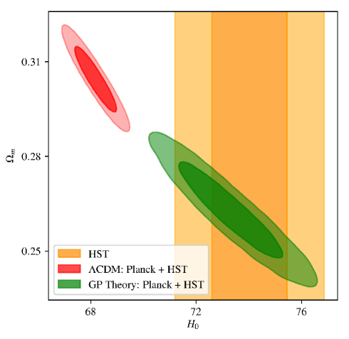
Figure 1: Combining all the data together, the GP model is able to make $H_{0}$ measurements compatible at 2-sigma with the MCMC results.

We also show in Fig. 2 the results for the same data sets having followed a slightly different approach by using CosmoMC. We can see that the two results are completely consistent. This result gives a check for the consistence of (either of) the code.

Figure 2: One and two-dimensional distributions of $s$, $H_{0}$ and $\Omega_{m}$ in Planck+ HST data sets, where the contour lines represent 68$\%$  and 95$\%$  C.L., respectively. The results obtained here via CosmoMC are shown to be consistent with the ones obtained by CLASS/Montepython. This test gives a strong check on the consistency of (either of) the code.

Table 2 shows the constraints to the parameters up to $95\%$ of C.L. Notice that for the parameter $\bar{\varphi}_{0}$ we could only give an upper bound (at 1-sigma). This is also shown in the triangular plot Fig. 3.

	Generalised Proca				$\boldsymbol{\Lambda\text{CDM}}$
Param	best-fit	mean$\pm\sigma$	95% lower	95% upper	best-fit	mean$\pm\sigma$	95% lower	95% upper
$s$	$0.3342$	$0.3455_{-0.14}^{+0.095}$	$0.1233$	$0.592$	-	-	-	-
$p_{2}$	$0.8344$	$0.4921_{-0.21}^{+0.11}$	$0.1885$	$0.8783$	-	-	-	-
$\log_{10}{\bar{\varphi}_{0}}$	$-0.7579$	$-0.5604_{nan}^{+nan}$	$nan$	$nan$	-	-	-	-
$H_{0}$	$73.48$	$73.34_{-1.3}^{+1.3}$	$70.79$	$75.94$	$68.26$	$68.18_{-0.53}^{+0.53}$	$67.13$	$69.25$
$\Omega_{m}$	$0.2607$	$0.2625_{-0.01}^{+0.0099}$	$0.2429$	$0.2824$	$0.3039$	$0.3045_{-0.0071}^{+0.0069}$	$0.2907$	$0.3186$

Table 2: Cosmological constraints for the parameters at 1$\sigma$ and 2$\sigma$ for both Generalized Proca theory and $\Lambda\text{CDM}$ confronted with Planck+HST data sets.

For the GP theory, the bestfit value gives $\chi^{2}=2773$, whereas $\Lambda\text{CDM}$ gives $\chi^{2}=2794.64$. Table 3 shows the effective $\chi^{2}$ for the individual experiments. That is, there is a remarkable betterment in the fitting of the GP theory in comparison with that of $\Lambda\text{CDM}$ with $|\Delta\chi^{2}|\sim 22$. We also give the triangular plots of the parameters in Fig. 3.

Experiments	$\chi^{2}$ effective
	Generalised Proca	$\boldsymbol{\Lambda\text{CDM}}$
Planck_highl_TTTEEE	2346.51	2348.98
Planck_lowl_EE	395.67	397.03
Planck_lowl_TT	21.82	22.87
Planck_lensing	8.45	9.21
hst	0.15	16.54
Total	2772.60	2794.64

Table 3: $\chi^{2}$ effective for individual experiments with the dataset of Planck + HST.

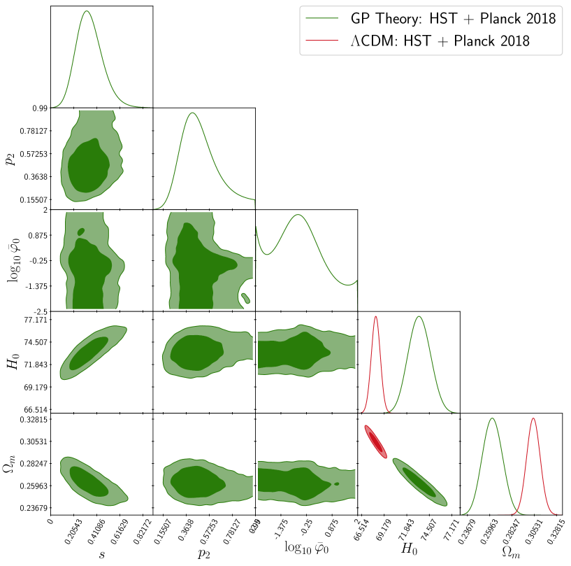
Figure 3: The triangular plot for the cosmological parameters for the Generalized Proca theory confronted with Planck + HST data sets.

IV.2 Planck, JLA, HST and BAO

We also check the cosmological constraints for the GP theory combining Planck, JLA, HST and BAO. Table 4 shows that constraints to the parameters and a comparison with the $\Lambda\text{CDM}$ values for $H_{0}$ and $\Omega_{m}$. We have found that the value of $s$ on using all the data is reduced. It is interesting to notice that the value of the $H_{0}$ has changed with in the $95\%$ C.L. in comparison with $\Lambda\text{CDM}$. However, within the GP theory, Planck data and local measurement of $H_{0}$ agree within 2 sigma (by this we mean that the 2$\sigma$ regions for Proca and the $H_{0}$ measurements overlap), as shown in Fig. 4.

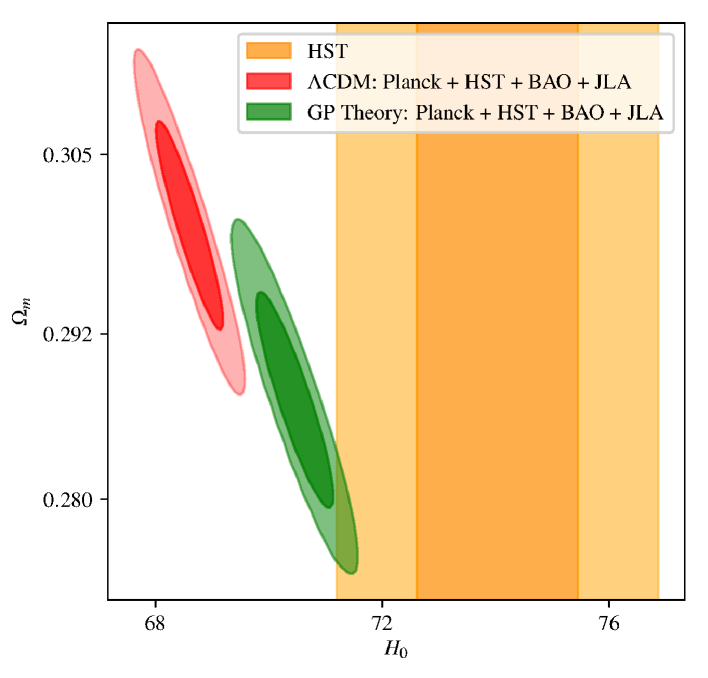
Figure 4: Combining all the data together, the GP model is able to make $H_{0}$ measurements compatible at 2-sigma with the MCMC results.

Therefore, GP is able to reduce the tension in the data we have considered. This behaviour sounds really promising and it should be checked against future data.

The parameter $\bar{\varphi}_{0}$ as in the previous case has a large degeneracy, and we can only give an upper bound (at 1-sigma) to it.

	Generalised Proca				$\boldsymbol{\Lambda\text{CDM}}$
Param	best-fit	mean$\pm\sigma$	95% lower	95% upper	best-fit	mean$\pm\sigma$	95% lower	95% upper
$s$	$0.172$	$0.1722_{-0.01}^{+0.013}$	$0.1432$	$0.1984$	-	-	-	-
$p_{2}$	$0.226$	$0.232_{-0.041}^{+0.038}$	$0.1392$	$0.3246$	-	-	-	-
$\log_{10}{\bar{\varphi}_{0}}$	$-0.2856$	$-1.492_{nan}^{+nan}$	$nan$	$nan$	-	-	-	-
$H_{0}$	$70.41$	$70.45_{-0.45}^{+0.45}$	$69.54$	$71.35$	$68.59$	$68.6_{-0.4}^{+0.4}$	$67.79$	$69.4$
$\Omega_{m}$	$0.2877$	$0.2873_{-0.0054}^{+0.0051}$	$0.2768$	$0.2977$	$0.3001$	$0.2999_{-0.0052}^{+0.005}$	$0.2896$	$0.3102$

Table 4: This table shows the cosmological constraints to the parameters for both the generalized Proca theory and $\Lambda\text{CDM}$ confronted with Planck + HST + BAO + JLA data sets.

For this theory we get a $\chi^{2}=3472$, which is again lower than that of $\Lambda\text{CDM}$, which is $\chi^{2}=3479$, resulting in difference of $|\Delta\chi^{2}|=7$. Table 5 shows the effective $\chi^{2}$ for the individual experiments. For this data set also we find that there is a preference of the GP theory over $\Lambda\text{CDM}$. It is evident from the table 5, that the improvement in effective $\chi^{2}$ of HST is done at the cost of a (partial) degradation of the effective $\chi^{2}$ of BAO and JLA. We show the triangular plot for the parameters in Fig. 5. Besides noticing the difference of $\chi^{2}$, we want to consider other statistical analysis to compare the two models. In particular, we select not only Akaike Information Criterion (AIC) but also AIC with a correction (which under certain conditions, is more accurate, especially for small sample sizes) (AICc) and Bayesian Information Criterion (BIC) to compare the two models Trotta:2008qt . The AICc criterion can be expressed by

$$AICc\equiv-2\ln L_{max}+2k+\frac{2k^{2}+2k}{n-k-1},$$ (59)

where $L_{max}\equiv p(d|\theta_{max},M)$ is the maximum likelihood value and $k$ is the number of free parameters in the model. Here, $n$ denotes the sample size of the simulation and it will lead AICc to converge to AIC when $n\to\infty$. Since $\chi^{2}=-2\ln L_{max}$ and GP just has one more free background parameter, $s$, than $\Lambda$CDM, we can get $\triangle AICc=\triangle AICc_{\Lambda CDM}-\triangle AICc_{GP}=20.031(4.321)$ in Planck+HST (Planck+HST+BAO+JLA) dataset. Since there is a large degeneracy for $\bar{\varphi}_{0}$ we can, without loss of generality, fix it to some value. On adding the perturbation parameter $p_{2}$, we find that $\triangle AICc=\triangle AICc_{\Lambda CDM}-\triangle AICc_{GP}=18.02(2.31)$. Even in this case, the value for $\triangle AICc$ shows preference for the GP theory compared to the $\Lambda$CDM model Arevalo:2016epc .

On the other hand, the Bayesian criterion is defined as

$$BIC\equiv-2\ln L_{max}+k\ln n.$$ (60)

The $\triangle BIC=\triangle BIC_{\Lambda CDM}-\triangle BIC_{GP}=5.65$. It shows the evidence against for our GP theory more close to the observational data than the $\Lambda$CDM in Planck+HST dataset. This result is consistent with our conclusion from the difference of $\chi^{2}$ in global fitting.

Experiments	$\chi^{2}$ effective
	Generalised Proca	$\boldsymbol{\Lambda\text{CDM}}$
Planck_highl_TTTEEE	2343.12	2346.06
Planck_lowl_EE	395.72	397.64
Planck_lowl_TT	22.43	23.01
Planck_lensing	9.59	8.74
JLA	685.36	683.04
bao_boss_dr12	5.60	3.39
bao_smallz_2014	3.87	2.03
hst	6.51	14.65
Total	3472.22	3478.55

Table 5: $\chi^{2}$ effective for individual experiments with the dataset of Planck + HST + BAO +JLA.

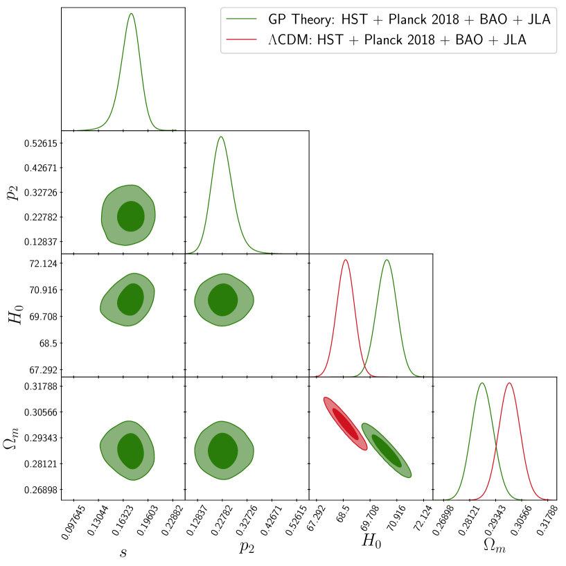
Figure 5: The triangular plot for the cosmological parameters for the Generalized Proca theory confronted with Planck + HST + BAO + JLA data sets.

In order to show the modification of GP Theory in the early universe, we compare the difference of CMB power spectra of the TT mode for GP Theory and $\Lambda$CDM with the observation we used above. In Fig. 6, the $\Lambda$CDM and GP Theory with the value of parameters are form best-fit value of Planck + HST + BAO + JLA data set. In the high-$\ell$ part of Fig. 6, we can find the GP is very close to $\Lambda$CDM and is with in the error-bars of Planck 2018 data Aghanim:2019ame . In the low-$\ell$, we can see the CMB value of GP Theory is smaller than $\Lambda$CDM when $\ell$ is smaller to 10. This difference in large scale structure shows the impact of the GP Theory’s initial condition in the early universe, but it is still under the error-bar and hard to be distinguished in present CMB observational data as shown in the figure. The lower panel of the Fig. 6 shows the relative difference of the $C_{\ell}^{TT}$ of GP theory with respect to $\Lambda$CDM. The difference is inside the error-bars.

Figure 6: CMB power spectra TT mode for the $\Lambda$CDM and GP Theory obtained using the bestfit parameters for both theories to the Planck + HST + BAO + JLA data set. The lower panel shows the relative difference of the $C_{\ell}^{TT}$ of GP theory with respect to $\Lambda$CDM. The error-bars are $1-\sigma$ from Planck 2018 TT power spectra.

V Conclusion

In this work we analyze extensively the viability of the generalized Proca theory up to cubic order in the Lagrangian from the cosmological observation. This study is particularly interesting in the context of the present day $H_{0}$ tension that is getting stronger. On considering Planck data and $H_{0}$ measurements alone, within this theory we do not see any tension between CMB data and the local measurement of the current expansion rate of the universe. In fact, we find a mean value for $H_{0}$ which exactly matches the value measured by $\text{H}0\text{LiCOW}$, namely $H_{0}=$$73.34_{-2.69}^{+2.46}$ at $95\%$ C.L. However, using BAO, HST, Planck and JLA together we see that the best fit for $H_{0}$ tends to be reduced, but still $H_{0}$ measurements are inside the 2 sigma contours. This indicates that the GP theory is able to reduce the tension below 2 sigma.

For this theory there are three more parameters $s,\,p_{2},\,\bar{\varphi}_{0}$ in comparison with standard $\Lambda\text{CDM}$ cosmological model. Out of which only $s$ affects the background dynamics. In particular, the parameter $s$ defines how much the theory deviates from $\Lambda\text{CDM}$ (which is obtained for the background in the limit $s\to 0$). In other words in the limit $s\rightarrow 0$ at the background level the theory becomes $\Lambda\text{CDM}$.

From the Planck + HST the parameter $s$ is constrained to be $s=0.334_{-0.211}^{+0.358}$ at $95\%$ C.L.  and on adding JLA and BAO we get $s=0.172_{-0.029}^{+0.026}$ at $95\%$ C.L.. The value of $s$ is in agreement with the previous study of the same theory with the CMB shift parameter deFelice:2017paw . However, our results are not only updated to the latest Planck and $H_{0}$ results, but the methodology is quite different. In deFelice:2017paw , Planck data were considered only through the constraints on the CMB-shift parameters. Instead in this study of ours, we have used the whole Planck data at once. Therefore, we can say we have confirmed the behaviour but such a step was a non-trivial one to show. In fact, other cases are known where the results from these two different methodologies do not agree with each other (see e.g. Dirian:2014bma ). The situation is also similar for the parameter $p_{2}$ at the $95\%$ C.L. for Planck+HST is $p_{2}=0.8344_{-0.6459}^{+0.4390}$ and with other data sets $p_{2}=0.226_{-0.087}^{+0.099}$. While the parameter $\bar{\varphi}_{0}$ does not converge at the $95\%$ C.L. there is large degeneracy for both cases. This is clearly shown in the Fig. 3.

Another remarkable point that has to be emphasized is that for the both MCMC run that is Planck+HST and Planck+HST+BAO+JLA the GP theory shows better fits in comparison with $\Lambda\text{CDM}$. The difference in $\chi^{2}$ is $|\Delta\chi^{2}|=22$ and $|\Delta\chi^{2}|=7$ respectively for Planck+HST and Planck+HST+BAO+JLA. This kind of behaviour is seen in other modified theories of gravity, for example Frusciante:2019puu (also see Li:2020ybr ; Li:2019ypi ). Nonetheless, we are able to show that Planck data and $H_{0}$ measurements agree with each other at 2-sigma within the GP theory. In future further exploring the reason behind the preference of models other than $\Lambda\text{CDM}$ will be of particular interest.

This study once again shows that the generalized proca theory up to the cubic order terms in the Lagrangian (as to have a speed of propagation for the gravitational wave $c_{T}\equiv 1$) reduces the tension of $H_{0}$ below 2-sigma in present data sets. This is mostly due to the particular background dynamics of $\Omega_{\text{DE}}$. This solution can be thought of as post recombination approach to the $H_{0}$ tension with modified gravity.

Appendix A Linear perturbation equations of motion

For clarity, here we give the full perturbation equations of motion. These same equation can be found in the C-code we have provided. After the discussion of section III, the modified equations of motion for the perturbations can be written as follows

$$\ddot{\bar{J}} = \left(3/2\,{\frac{{\bar{\varphi}}\,{a}^{3}\left(p+1\right){\Xi_{\rm T}}}{{p}^{2}{{\mathcal{H}}}^{2}\left({\Omega_{\rm DE}}\,s+1\right)}}-2\,{\frac{{\Omega_{\rm DE}}\,as}{{\bar{\varphi}}}}\right){\dot{\phi}}-{\frac{{\bar{\varphi}}\,a\left(p+1\right){\dot{\phi}}}{p}}$$ (61)

$$+ \left(-3\,{\frac{\left(ps-1\right){a}^{2}{k}^{2}{{\bar{\varphi}}}^{2}{\Xi_{\rm T}}}{p{\mathcal{H}}\left(6\,{{\mathcal{H}}}^{2}{p}^{2}s{\Omega_{\rm DE}}+{k}^{2}{{\bar{\varphi}}}^{2}\right)\left({\Omega_{\rm DE}}\,s+1\right)}}-2\,{\frac{{k}^{2}{\mathcal{H}}{{\bar{\varphi}}}^{2}}{6\,{{\mathcal{H}}}^{2}{p}^{2}s{\Omega_{\rm DE}}+{k}^{2}{{\bar{\varphi}}}^{2}}}\right){\dot{\bar{J}}}$$

$$+ \left(-{\frac{{a}^{2}\left({k}^{4}\left(-1/2+\left(s+1/2\right)p\right){{\bar{\varphi}}}^{4}+3\,{k}^{2}{\Omega_{\rm DE}}\,{p}^{2}s{{\mathcal{H}}}^{2}\left(p+2\right){{\bar{\varphi}}}^{2}+18\,{{\Omega_{\rm DE}}}^{2}{p}^{4}{s}^{2}{{\mathcal{H}}}^{4}\right){\Xi_{\rm T}}}{{p}^{2}{{\mathcal{H}}}^{2}{{\bar{\varphi}}}^{2}\left(6\,{{\mathcal{H}}}^{2}{p}^{2}s{\Omega_{\rm DE}}+{k}^{2}{{\bar{\varphi}}}^{2}\right)\left({\Omega_{\rm DE}}\,s+1\right)}}\right.$$

$$- \left.2/3\,{\frac{\left(1/2\,{k}^{2}{{\bar{\varphi}}}^{4}+{\Omega_{\rm DE}}\,ps\left(-3\,{{\mathcal{H}}}^{2}p+{k}^{2}\right){{\bar{\varphi}}}^{2}+6\,{{\Omega_{\rm DE}}}^{2}{p}^{3}{s}^{2}{{\mathcal{H}}}^{2}\right){k}^{2}}{p{{\bar{\varphi}}}^{2}\left(6\,{{\mathcal{H}}}^{2}{p}^{2}s{\Omega_{\rm DE}}+{k}^{2}{{\bar{\varphi}}}^{2}\right)}}\right){\bar{J}}$$

$$+ \left(-3\,{\frac{{\bar{\varphi}}\,{a}^{3}\left(p+1\right)\left({k}^{2}{{\bar{\varphi}}}^{2}ps-1/2\,{k}^{2}{{\bar{\varphi}}}^{2}+3\,{{\mathcal{H}}}^{2}{p}^{2}s{\Omega_{\rm DE}}\right){\Xi_{\rm T}}}{{p}^{2}{\mathcal{H}}\left(6\,{{\mathcal{H}}}^{2}{p}^{2}s{\Omega_{\rm DE}}+{k}^{2}{{\bar{\varphi}}}^{2}\right)\left({\Omega_{\rm DE}}\,s+1\right)}}\right.$$

$$+ \left.{\frac{a\left(-36\,{p}^{2}{\Omega_{\rm DE}}\,\left(\left(p/2+1/2\right){{\bar{\varphi}}}^{2}+ps{\Omega_{\rm DE}}\right)s{{\mathcal{H}}}^{4}+6\,{{\bar{\varphi}}}^{2}\left(\left(-3/2\,p-3/2\right){{\bar{\varphi}}}^{2}+ps{\Omega_{\rm DE}}\,\left(p-1\right)\right){k}^{2}{{\mathcal{H}}}^{2}+{k}^{4}{{\bar{\varphi}}}^{4}\right)}{3p{\mathcal{H}}{\bar{\varphi}}\,\left(6\,{{\mathcal{H}}}^{2}{p}^{2}s{\Omega_{\rm DE}}+{k}^{2}{{\bar{\varphi}}}^{2}\right)}}\right)\psi$$

$$+ \left(\frac{9}{2}{\frac{(p+1){\bar{\varphi}}{a}^{5}\left(3{{\mathcal{H}}}^{2}{p}^{2}s{\Omega_{\rm DE}}\,({\Omega_{\rm DE}}s+1)-6s{\Omega_{\rm DE}}{{\mathcal{H}}}^{2}({\Omega_{\rm DE}}{s}^{2}-1){p}^{3}+{k}^{2}{{\bar{\varphi}}}^{2}(s+1)p-1/2\,{k}^{2}{{\bar{\varphi}}}^{2}\left({\Omega_{\rm DE}}\,s+1\right)\right){{\Xi_{\rm T}^{2}}}}{\left({\Omega_{\rm DE}}\,s+1\right)^{3}\left(6\,{{\mathcal{H}}}^{2}{p}^{2}s{\Omega_{\rm DE}}+{k}^{2}{{\bar{\varphi}}}^{2}\right){{\mathcal{H}}}^{3}{p}^{3}}}\right.$$

$$+ {\frac{{a}^{3}\left({k}^{4}\left(-1/2+\left(s+1/2\right)p\right){{\bar{\varphi}}}^{4}+3\,\left(-6\,{p}^{2}{{\mathcal{H}}}^{2}+\left(-6\,{{\mathcal{H}}}^{2}+{k}^{2}\right)p+2\,{k}^{2}\right){p}^{2}{\Omega_{\rm DE}}\,{{\mathcal{H}}}^{2}s{{\bar{\varphi}}}^{2}+18\,{{\Omega_{\rm DE}}}^{2}{p}^{4}{s}^{2}{{\mathcal{H}}}^{4}\right){\Xi_{\rm T}}}{{\bar{\varphi}}\,{p}^{3}{{\mathcal{H}}}^{3}\left(6\,{{\mathcal{H}}}^{2}{p}^{2}s{\Omega_{\rm DE}}+{k}^{2}{{\bar{\varphi}}}^{2}\right)\left({\Omega_{\rm DE}}\,s+1\right)}}$$

$$- \left.2\,{\frac{{\bar{\varphi}}\,{a}^{3}\left(p+1\right){\Xi_{r}}}{{p}^{2}{\mathcal{H}}\left({\Omega_{\rm DE}}\,s+1\right)}}+2/3\,{\frac{a\left(1/2\,{k}^{2}{{\bar{\varphi}}}^{4}+{\Omega_{\rm DE}}\,ps\left(-3\,{{\mathcal{H}}}^{2}p+{k}^{2}\right){{\bar{\varphi}}}^{2}+6\,{{\Omega_{\rm DE}}}^{2}{p}^{3}{s}^{2}{{\mathcal{H}}}^{2}\right){k}^{2}}{{p}^{2}{\mathcal{H}}{\bar{\varphi}}\,\left(6\,{{\mathcal{H}}}^{2}{p}^{2}s{\Omega_{\rm DE}}+{k}^{2}{{\bar{\varphi}}}^{2}\right)}}\right)\phi\,,$$

$$\dot{\phi} = -1/4\,{\frac{\left(-4/3\,{{\Omega_{\rm DE}}}^{2}{p}^{2}{s}^{2}{{\mathcal{H}}}^{2}-4/3\,{{\mathcal{H}}}^{2}{p}^{2}s{\Omega_{\rm DE}}+{a}^{2}{{\bar{\varphi}}}^{2}{\Xi_{\rm T}}\,\left(p+1\right)\right)s{\Omega_{\rm DE}}\,{k}^{2}\phi}{{\mathcal{H}}\left({\Omega_{\rm DE}}\,s+1\right)^{2}p\left({{\mathcal{H}}}^{2}{p}^{2}s{\Omega_{\rm DE}}+1/6\,{k}^{2}{{\bar{\varphi}}}^{2}\right)}}$$

References

- [1] Jose Luis Bernal, Licia Verde, and Adam G. Riess. The trouble with . JCAP, 1610(10):019, 2016.
- [2] L. Verde, T. Treu, and A. G. Riess. Tensions between the Early and the Late Universe. In Nature Astronomy 2019, 2019.
- [3] N. Aghanim et al. Planck 2018 results. VI. Cosmological parameters. 2018.
- [4] N. Aghanim et al. Planck intermediate results. LI. Features in the cosmic microwave background temperature power spectrum and shifts in cosmological parameters. Astron. Astrophys., 607:A95, 2017.
- [5] T. M. C. Abbott et al. Dark Energy Survey Year 1 Results: A Precise H0 Estimate from DES Y1, BAO, and D/H Data. Mon. Not. Roy. Astron. Soc., 480(3):3879–3888, 2018.
- [6] Adam G. Riess, Stefano Casertano, Wenlong Yuan, Lucas M. Macri, and Dan Scolnic. Large Magellanic Cloud Cepheid Standards Provide a 1% Foundation for the Determination of the Hubble Constant and Stronger Evidence for Physics beyond CDM. Astrophys. J., 876(1):85, 2019.
- [7] Kenneth C. Wong et al. H0LiCOW XIII. A 2.4% measurement of from lensed quasars: tension between early and late-Universe probes. 2019.
- [8] M. J. Reid, J. A. Braatz, J. J. Condon, L. J. Greenhill, C. Henkel, and K. Y. Lo. The Megamaser Cosmology Project: I. VLBI observations of UGC 3789. Astrophys. J., 695:287–291, 2009.
- [9] Wendy L. Freedman et al. The Carnegie-Chicago Hubble Program. VIII. An Independent Determination of the Hubble Constant Based on the Tip of the Red Giant Branch. 2019.
- [10] Lloyd Knox and Marius Millea. Hubble constant hunter’s guide. Phys. Rev. D, 101(4):043533, 2020.
- [11] Vivian Poulin, Tristan L. Smith, Tanvi Karwal, and Marc Kamionkowski. Early Dark Energy Can Resolve The Hubble Tension. Phys. Rev. Lett., 122(22):221301, 2019.
- [12] S. Nojiri, S. D. Odintsov, and V. K. Oikonomou. Modified Gravity Theories on a Nutshell: Inflation, Bounce and Late-time Evolution. Phys. Rept., 692:1–104, 2017.
- [13] Y. Fujii and K. Maeda. The scalar-tensor theory of gravitation. Cambridge Monographs on Mathematical Physics. Cambridge University Press, 2007.
- [14] Lavinia Heisenberg. Generalization of the Proca Action. JCAP, 1405:015, 2014.
- [15] Lavinia Heisenberg. Generalised Proca Theories. In Proceedings, 52nd Rencontres de Moriond on Gravitation (Moriond Gravitation 2017): La Thuile, Italy, March 25-April 1, 2017, pages 233–241, 2017.
- [16] Antonio De Felice, Lavinia Heisenberg, Ryotaro Kase, Shinji Mukohyama, Shinji Tsujikawa, and Ying-li Zhang. Cosmology in generalized Proca theories. JCAP, 1606(06):048, 2016.
- [17] B. P. Abbott et al. GW170817: Observation of Gravitational Waves from a Binary Neutron Star Inspiral. Phys. Rev. Lett., 119(16):161101, 2017.
- [18] A. Goldstein et al. An Ordinary Short Gamma-Ray Burst with Extraordinary Implications: Fermi-GBM Detection of GRB 170817A. Astrophys. J., 848(2):L14, 2017.
- [19] Shintaro Nakamura, Antonio De Felice, Ryotaro Kase, and Shinji Tsujikawa. Constraints on massive vector dark energy models from integrated Sachs-Wolfe-galaxy cross-correlations. Phys. Rev., D99(6):063533, 2019.
- [20] Antonio De Felice, Lavinia Heisenberg, and Shinji Tsujikawa. Observational constraints on generalized Proca theories. Phys. Rev., D95(12):123540, 2017.
- [21] Diego Blas, Julien Lesgourgues, and Thomas Tram. The Cosmic Linear Anisotropy Solving System (CLASS) II: Approximation schemes. JCAP, 1107:034, 2011.
- [22] Masroor C. Pookkillath, Antonio De Felice, and Shinji Mukohyama. Baryon Physics and Tight Coupling Approximation in Boltzmann Codes. Universe, 6:6, 2020.
- [23] Thejs Brinckmann and Julien Lesgourgues. MontePython 3: boosted MCMC sampler and other features. Phys. Dark Univ., 24:100260, 2019.
- [24] Benjamin Audren, Julien Lesgourgues, Karim Benabed, and Simon Prunet. Conservative Constraints on Early Cosmology: an illustration of the Monte Python cosmological parameter inference code. JCAP, 1302:001, 2013.
- [25] Antony Lewis and Sarah Bridle. Cosmological parameters from CMB and other data: A Monte Carlo approach. Phys. Rev., D66:103511, 2002.
- [26] Bernard F. Schutz and Rafael Sorkin. Variational aspects of relativistic field theories, with application to perfect fluids. Annals Phys., 107:1–43, 1977.
- [27] Antonio De Felice, Jean-Marc Gerard, and Teruaki Suyama. Cosmological perturbations of a perfect fluid and noncommutative variables. Phys. Rev., D81:063527, 2010.
- [28] N. Aghanim et al. Planck 2018 results. V. CMB power spectra and likelihoods. 2019.
- [29] Y. Akrami et al. Planck 2018 results. IX. Constraints on primordial non-Gaussianity. 2019.
- [30] Y. Akrami et al. Planck 2018 results. X. Constraints on inflation. 2018.
- [31] N. Aghanim et al. Planck 2018 results. VIII. Gravitational lensing. 2018.
- [32] Florian Beutler, Chris Blake, Matthew Colless, D. Heath Jones, Lister Staveley-Smith, Lachlan Campbell, Quentin Parker, Will Saunders, and Fred Watson. The 6dF Galaxy Survey: Baryon Acoustic Oscillations and the Local Hubble Constant. Mon. Not. Roy. Astron. Soc., 416:3017–3032, 2011.
- [33] Ashley J. Ross, Lado Samushia, Cullan Howlett, Will J. Percival, Angela Burden, and Marc Manera. The clustering of the SDSS DR7 main Galaxy sample – I. A 4 per cent distance measure at . Mon. Not. Roy. Astron. Soc., 449(1):835–847, 2015.
- [34] Shadab Alam et al. The clustering of galaxies in the completed SDSS-III Baryon Oscillation Spectroscopic Survey: cosmological analysis of the DR12 galaxy sample. Mon. Not. Roy. Astron. Soc., 470(3):2617–2652, 2017.
- [35] M. Betoule et al. Improved cosmological constraints from a joint analysis of the SDSS-II and SNLS supernova samples. Astron. Astrophys., 568:A22, 2014.
- [36] Roberto Trotta. Bayes in the sky: Bayesian inference and model selection in cosmology. Contemp. Phys., 49:71–104, 2008.
- [37] Fabiola Arevalo, Antonella Cid, and Jorge Moya. AIC and BIC for cosmological interacting scenarios. Eur. Phys. J., C77(8):565, 2017.
- [38] Yves Dirian, Stefano Foffa, Martin Kunz, Michele Maggiore, and Valeria Pettorino. Non-local gravity and comparison with observational datasets. JCAP, 1504(04):044, 2015.
- [39] Noemi Frusciante, Simone Peirone, Luis Atayde, and Antonio De Felice. Phenomenology of the generalized cubic covariant Galileon model and cosmological bounds. Phys. Rev. D, 101(6):064001, 2020.
- [40] Xiaolei Li and Arman Shafieloo. Generalised Emergent Dark Energy Model: Confronting and PEDE. 2020.
- [41] Xiaolei Li and Arman Shafieloo. A Simple Phenomenological Emergent Dark Energy Model can Resolve the Hubble Tension. Astrophys. J., 883(1):L3, 2019. [Astrophys. J. Lett.883,L3(2019)].