No Chaos in Dixon’s System

Abstract

The so-called Dixon system is often cited as an example of a two-dimensional (continuous) dynamical system that exhibits chaotic behaviour, if its two parameters take their value in a certain domain. We provide first a rigorous proof that there is no chaos in Dixon’s system. Then we perform a complete bifurcation analysis of the system showing that the parameter space can be decomposed into sixteen different regions in each of which the system exhibits qualitatively the same behaviour. In particular, we prove that in some regions two elliptic sectors with infinitely many homoclinic orbits exist.

1 Introduction

Cummings et al. [1992] derived a model for the magnetic field of neutron stars consisting of three autonomous ordinary differential equations. One of the equations can be easily decoupled so that the core of the model is given by a two-dimensional dynamical system depending on two positive real parameters $a$ and $b$ (see (1) below) which we will call CDK system. In numerical simulations of this system, Cummings et al. observed for $0<a,b<1$ a complicated dynamics (which matches some astronomical observations) and suspected a chaotic behaviour. In a subsequent article Dixon et al. [1993], they reported – based on additional numerical experiments – a positive Lyapunov exponent as a further indication of chaos.

Since the Poincaré-Bendixson Theorem excludes chaos in two-dimensional continuous dynamical systems, these findings raised some interest. Dixon et al. [1993] already stated that the CDK system was not a counterexample, as the assumptions of the theorem were violated. In fact, they were always very careful in their formulations: they used the word chaos only with quotation marks and noted already in their first article that classical conditions for chaos were not satisfied. In a further article, Dixon [1995] completely avoided the use of this term and coined instead the phrase “piecewise deterministic dynamics”. Nevertheless, under the name Dixon’s system (which is a bit unfair towards the other authors of these works) their differential equations are repeatedly cited as an example of a chaotic system (see e. g. Sprott [2010]), although Alvarez-Ramirez et al. [2005] already clearly indicated that the seemingly chaotic behaviour is simply due to the existence of two elliptic sectors with infinitely many homoclinic orbits. We will briefly indicate that also in a logarithmic variant of the CDK system proposed by Sprott [2010] as a further “chaotic” system in the plane no chaos appears.

In this article, we will first exhibit some shortcomings of the analysis in Dixon et al. [1993]. Indeed, their argument against the applicability of the Poincaré-Bendixson Theorem is inconsistent and furthermore relies on a simplified version of the theorem. Using a geometric approach based on singularity theory, we will then provide a rigorous proof that also a refined version cannot be directly applied to the CDK system. We will show that one can derive a polynomial vector field possessing the same integral curves as the CDK system with the origin as a degenerate stationary point. This allows us a rigorous qualitative analysis of the solution behaviour in the neighbourhood of the origin.

Cummings et al. [1992] distinguished in their numerical studies four different regions in the parameter space. We will show that a rigorous classification leads actually to sixteen different regions, if one also takes the behaviour at infinity into account. It turns out that although the two parameters in the system are from a physical point of view of essentially the same nature, they play mathematically a very different role. In particular, the emergence of the homoclinic orbits is completely controlled by one of them alone.

2 The CDK System and the Poincaré-Bendixson Theorem

In their work on the magnetic field of neutron stars, Cummings et al. [1992] derived the following planar dynamical system

$$\dot{x}=\frac{xy}{x^{2}+y^{2}}-ax\,,\qquad\dot{y}=\frac{y^{2}}{x^{2}+y^{2}}-by+b-1$$ (1)

depending on two positive parameters $a,b>0$ as decoupled part of a three-dimensional model. For the physical interpretation of the model, we refer to their article. The analysis of the stationary points of this planar system and of their stability leads naturally to case distinctions whether zero, one or two of the parameters have a value larger than $1$. In numerical simulations, the case $0<a,b<1$ showed a complicated behaviour that Cummings et al. [1992] suspected to be chaotic.

In the subsequent article, Dixon et al. [1993] provided a closer analysis of this case giving further numerical evidence for a highly irregular dynamics resembling chaos. They also discussed whether their model represented a counterexample to the Poincaré-Bendixson Theorem. Obviously, the right hand side of (1) consists of rational functions with a pole at the origin. Dixon et al. [1993] showed that its gradient does not possess a well-defined limit for $(x,y)\rightarrow(0,0)$ and concluded that therefore the system was not $\mathcal{C}^{1}$ as assumed in the Poincaré-Bendixson Theorem. This argument is erroneous in at least two respects. Firstly, the cited version of the Poincaré-Bendixson Theorem assumes a dynamical system defined on the whole plane, whereas the right hand side of (1) is obviously not defined at the origin. Secondly, it makes no sense to study the differentiability of a function at a point where it is not defined. In fact, it is easy to verify that the right hand side of (1) itself does not possess a well defined limit for $(x,y)\rightarrow(0,0)$.

We will use here the following version of the Poincaré-Bendixson Theorem, as it can e. g.  be found in the text book by Perko [2001, Thm. 1, Sect. 3.7].

Theorem 2.1 (Poincaré-Bendixson).

Let the autonomous dynamical system $\dot{\mathbf{x}}=\mathbf{f}(\mathbf{x})$ be defined on an open subset $\Omega\subseteq\mathbbm{R}^{2}$ with $\mathbf{f}\in\mathcal{C}^{1}(\Omega,\mathbbm{R}^{2})$. Assume that a forward trajectory lies completely in a compact subset $\mathcal{K}\subset\Omega$. Then the $\omega$-limit set of the trajectory contains either stationary points of the system or it is a periodic orbit.

In the case of the CDK system (1), the obvious choice for the open set $\Omega$ is the punctured plane $\Omega=\mathbbm{R}^{2}\setminus\{0\}$. The decisive question for the applicability of Theorem 2.1 is now whether we can find an enclosing compact set $\mathcal{K}\subset\Omega$ for every bounded forward trajectory. Only if this is the case, we can exclude chaos by applying Theorem 2.1 directly to (1). However, we will show in Section 3 as a by-product of our geometric analysis of (1) that this is not possible if the values of the parameters $(a,b)$ lie in certain regions of the parameter space. More precisely, we will prove that for such parameter values there exist infinitely many trajectories starting arbitrarily close to the origin and approaching for $t\rightarrow\infty$ the origin again arbitrarily close. Obviously, any compact set $\mathcal{K}$ enclosing such a trajectory must contain the origin and thus cannot be a subset of $\Omega$. On the other hand, it is also clear that none of these trajectories exhibit a chaotic behaviour, as each of them has an $\omega$-limit set consisting simply of the origin.

However, even in this refined form this argument only shows that Theorem 2.1 is not directly applicable to the CDK system in the form (1). The key idea of our geometric analysis in Section 3 will be to study instead of the rational system (1) a polynomial vector field which is defined on the entire plane $\mathbbm{R}^{2}$ and which is trajectory equivalent to (1) on $\Omega$. The application of Theorem 2.1 to this system is straightforward and shows immediately that the CDK system cannot exhibit chaos. The origin will be a degenerate stationary point for this polynomial vector field and thus it becomes a standard problem in dynamical systems theory to study the behaviour of solutions of (1) close to the origin.

3 A Geometric Approach to the CDK System

We follow here an approach pioneered by Vessiot [1924] who showed how the analysis of an arbitrary system of differential equations can be reduced to the study of (systems of) vector fields (see Seiler [2010] and references therein for a modern representation). In the case of ordinary differential equations, this approach allows to transform implicit equations into explicit ones. In the context of the singularity theory of ordinary differential equations – see Arnold [1988] for a simple introduction – this approach is standard (however, without being attributed to Vessiot). In the literature, the arising theory is often named after Cartan. Following Fackerell [1985], we think that this is not appropriate, as Cartan worked almost exclusively with differential forms and not with vector fields. Quasi-linear equations show in this context a special behaviour with properties not present in arbitrary non-linear equations. Although this phenomenon has a very simple explanation, it seems that it was exhibited for the first time only fairly recently in Seiler [2013]. For a more detailed analysis see the recent work Seiler & Seiß [2018].

In the geometric theory of differential equations (see Seiler [2010] and references therein for an in-depth introduction into at least the regular case), a differential equation is modelled as a fibred submanifold of an appropriate jet bundle. To be able to study also singularities, we take a more general point of view and define a differential equation as a subvariety of the jet bundle such that its image under the canonical projection to the space of independent variables is dense.

More precisely, we take for the purpose of this article which studies exclusively first-order ordinary differential equations with polynomial nonlinearities as underlying base space $\mathbbm{R}$ and consider jets of local functions $\mathbbm{R}\rightarrow\mathbbm{R}^{n}$. Local coordinates of the first jet bundle $\mathcal{J}_{1}(\mathbbm{R},\mathbbm{R}^{n})\cong\mathbbm{R}\times\mathbbm{R}^{n}\times\mathbbm{R}^{n}$ are then denoted by $(t,\mathbf{x},\dot{\mathbf{x}})$. We have two canonical projections $\pi^{1}_{0}:\mathcal{J}_{1}(\mathbbm{R},\mathbbm{R}^{n})\rightarrow\mathbbm{R}\times\mathbbm{R}^{n}$ and $\pi^{1}:\mathcal{J}_{1}(\mathbbm{R},\mathbbm{R}^{n})\rightarrow\mathbbm{R}$. An algebraic differential equation is a subvariety $\mathcal{R}_{1}\subseteq\mathcal{J}_{1}(\mathbbm{R},\mathbbm{R}^{n})$ such that $\pi^{1}(\mathcal{R}_{1})$ lies dense in $\mathbbm{R}$. Thus we consider exclusively systems of the form $\mathbf{F}(t,\mathbf{x},\dot{\mathbf{x}})=0$ where the components of $\mathbf{F}$ are polynomials.

We distinguish two kinds of singularities of such a differential equation. An algebraic singularity is a point $\rho\in\mathcal{R}_{1}$ which is not smooth, i. e. a singular point in the sense of algebraic geometry. A geometric singularity is a smooth point $\rho\in\mathcal{R}_{1}$ which is critical for the restricted projection $\pi^{1}|_{\mathcal{R}_{1}}$, i. e. a singular point in the sense of differential topology. While much is known about the local solution behaviour around geometric singularities (see e. g. Arnold [1988] for an elementary introduction to the case of scalar first-order equations), not much can be found in the literature about algebraic singularities.

The contact distribution $\mathcal{C}^{(1)}$ of $\mathcal{J}_{1}(\mathbbm{R},\mathbbm{R}^{n})$ is generated by the $n+1$ vector fields

$$C_{\mathrm{trans}}=\partial_{t}+\sum_{i=1}^{n}\dot{x}_{i}\partial_{x_{i}}\,,\qquad C_{i}=\partial_{\dot{x}_{i}}\,.$$ (2)

The first field is transversal with respect to the projection $\pi^{1}$ (and essentially encodes the chain rule), whereas the remaining $n$ fields $C_{i}$ span the vertical bundle for the projection $\pi^{1}_{0}$. Given an algebraic differential equation $\mathcal{R}_{1}\subseteq\mathcal{J}_{1}(\mathbbm{R},\mathbbm{R}^{n})$, we define the Vessiot space at a smooth point $\rho\in\mathcal{R}_{1}$ as $\mathcal{V}_{\rho}[\mathcal{R}_{1}]=T_{\rho}\mathcal{R}_{1}\cap\mathcal{C}^{(1)}_{\rho}$, i. e. as that part of the contact distribution that is tangential to $\mathcal{R}_{1}$. $\mathcal{V}_{\rho}[\mathcal{R}_{1}]$ is obviously a linear space whose dimension can vary with the point $\rho$. It is easy to see that on a (Zariski) open subset of $\mathcal{R}_{1}$ the Vessiot spaces define a smooth regular distribution. By a certain abuse of language, we call the whole family of Vessiot spaces the Vessiot distribution of $\mathcal{R}_{1}$.

We call an integral curve $\mathcal{S}\subseteq\mathcal{R}_{1}$ of the Vessiot distribution $\mathcal{V}[\mathcal{R}_{1}]$ a generalised solution of $\mathcal{R}_{1}$ and its projection $\pi^{1}_{0}(\mathcal{S})$ a geometric solution. If the function $\mathbf{s}(t)$ is a solution of $\mathcal{R}_{1}$ in the classical sense, then its graph is a geometric solution and the curve defined by all points $\bigl{(}t,\mathbf{s}(t),\dot{\mathbf{s}}(t)\bigr{)}$ a generalised solution. Note, however, that not every geometric solution is necessarily the graph of a function.

Consider now a quasi-linear system of the form $A(t,\mathbf{x})\dot{\mathbf{x}}=\mathbf{r}(t,\mathbf{x})$ where we assume for simplicity that the matrix $A$ is almost everywhere non-singular and that at those points where it is singular the rank drops only by one. Then it is shown in Seiler [2013] that outside of certain singularities the generator of the Vessiot distribution is projectable to $\mathbbm{R}\times\mathbbm{R}^{n}$ and yields there the vector field $Y=\delta(t,\mathbf{x})\partial_{t}+\bigl{(}C(t,\mathbf{x})\mathbf{r}(t,\mathbf{x})\bigr{)}^{t}\partial_{\mathbf{x}}$ where $\delta(t,\mathbf{x})=\det{A(t,\mathbf{x})}$ and $C(t,\mathbf{x})$ is the adjunct of $A(t,\mathbf{x})$. Strictly speaking, the projected vector field $Y$ is defined only on the subset $\pi^{1}_{0}(\mathcal{R}_{1})\subseteq\mathbbm{R}\times\mathbbm{R}^{n}$. However, from the above explicit expression one can see that $Y$ can be analytically extended to all points on $\mathbbm{R}\times\mathbbm{R}^{n}$ where $\delta$ and $C$ are defined. If we assume that $A$ and $\mathbf{r}$ are polynomial in their arguments, then obviously this means that we may consider $Y$ as a vector field on the whole space $\mathbbm{R}\times\mathbbm{R}^{n}$.

We call an invariant curve of the vector field $Y$ a weak geometric solution. Indeed, any geometric solution is also a weak one; however, parts of weak geometric solution may correspond to the graph of a function which is continuous but not differentiable. In particular, any integral curve of the quasi-linear system is also an invariant curve of this vector field. Thus the analysis of the original implicit problem can be reduced to the study of the vector field $Y$, i. e. an explicit autonomous differential equation. For more details about this geometric approach we refer again to Seiler & Seiß [2018].

For the application of the above sketched ideas to the CDK system (1), we work in the jet bundle $\mathcal{J}_{1}(\mathbbm{R},\mathbbm{R}^{2})$ with local coordinates $(t,x,y,\dot{x},\dot{y})$. Its contact distribution is locally generated by the following three vector fields

$$C_{\mathrm{trans}}=\partial_{t}+\dot{x}\partial_{x}+\dot{y}\partial_{y}\,,\qquad C_{x}=\partial_{\dot{x}}\,,\qquad C_{y}=\partial_{\dot{y}}\,.$$ (3)

Instead of working with (1), we prefer to rewrite the system in the quasi-linear form

$$(x^{2}+y^{2})\dot{x} =xy-a(x^{3}+xy^{2})\,,$$ (4)

$$(x^{2}+y^{2})\dot{y} =y^{2}-(by-b+1)(x^{2}+y^{2})\,,$$

as these equations are also defined at points with $x=y=0$, since they are polynomial in all variables. Nevertheless, even in this implict form these points are problematic. As one can easily check with the Jacobian of (4), the zero set of (4) is not a submanifold of $\mathcal{J}_{1}(\mathbbm{R},\mathbbm{R}^{2})$, but a three-dimensional variety for which all these points represent a singularity in the sense of algebraic geometry.

For the construction of the Vessiot distribution of the differential equation $\mathcal{R}_{1}$ defined by (4), we take a general vector field $X=\alpha C_{\mathrm{trans}}+\beta C_{x}+\gamma C_{y}$ in the contact distribution $\mathcal{C}^{(1)}$ with yet undetermined coefficients and check when it is tangential to $\mathcal{R}_{1}$. This yields the equations

$$(x^{2}+y^{2})\beta =\bigl{(}(y-3ax^{2}-ay^{2})\dot{x}+(x-2axy)\dot{y}\bigr{)}\alpha\,,$$ (5)

$$(x^{2}+y^{2})\gamma =-\bigl{(}2(by-b+1)x\dot{x}+b(3y+2)y\dot{y}\bigr{)}\alpha\,.$$

For the projected vector field $Y=(\pi^{1}_{0})_{*}(X)$ we only need a value for $\alpha$ which obviously may be chosen as $x^{2}+y^{2}$. Using the equations (4), we thus obtain

$$Y=(x^{2}+y^{2})\partial_{t}+\bigl{(}xy-a(x^{3}+xy^{2})\bigr{)}\partial_{x}+\bigl{(}y^{2}-(by-b+1)(x^{2}+y^{2})\bigr{)}\partial_{y}\,.$$ (6)

Note that, strictly speaking, the Vessiot spaces are defined only at smooth points, i.e. in our example the vector field $X$ is not defined at all points with $x=y=0$, as these are singularities in the sense of algebraic geometry. However, it is easy to see that the projected vector field $Y$ can be analytically extended to the whole of $\mathbbm{R}^{3}$, so that we can ignore the fact that these points are algebraic singularities.

For analysing the phase portrait of (4), the dynamics in $t$-direction is irrelevant, as it simply describes a reparametrisation of time, and we can concentrate on the planar dynamical system defined by the second and third component of $Y$

$$\dot{x}=xy-a(x^{3}+xy^{2})\,,\quad\dot{y}=y^{2}-(by-b+1)(x^{2}+y^{2})\,,$$ (7)

where the dot denotes now the differentiation with respect to some parameter $\tau$. Alternatively, one may derive the same system via a time reparametrisation in (4) and consider $\tau$ as the new time variable. We prefer our approach via singularity theory, as its interpretation is more transparent in situations where the reparametrisation does not define a bijective function.

Obviously, the polynomial dynamical system (7) is defined on the whole plane $\mathbbm{R}^{2}$ and outside of the origin its trajectories coincide with the ones of the CDK system (4). The Poincaré-Bendixson Theorem even in its most elementary form trivially applies to (7) and thus we can rigorously exclude the possibility of any form of chaotic dynamics in the CDK system. It is easy to see that the origin is a stationary point of (7) and that the Jacobian of the system vanishes at the origin. Thus we are in the case of a nilpotent stationary point requiring a careful analysis via blow-ups to determine the local solution behaviour.

4 Stationary Points of the CDK System

4.1 The Set of Stationary Points

In this section we determine the set of stationary points of the dynamical system in dependence of the parameters $a,b\in\mathbb{R}_{>0}$. This set is given by the zero set of the polynomial system

$$x(y-ay^{2}-ax^{2}) = 0,$$ (8a)

$$-by^{3}-byx^{2}+by^{2}+(b-1)x^{2} = 0.$$ (8b)

In order to describe its solution set it is useful to distinguish between the cases $x=0$ and $x\neq 0$.

For $x=0$, (8a) is always satisfied and (8b) reduces to $-by^{3}+by^{2}=by^{2}(1-y)=0$. Solving this equation, we obtain the two zeros $(x,y)=(0,0)$ and $(x,y)=(0,1)$ which are independent from the parameter values. This means that the stationary points of the system with $x=0$ for all $a$,$b\in\mathbb{R}_{>0}$ are $s_{1}:=(0,0)$ and $s_{2}:=(0,1)$.

For $x\neq 0$, (8a) is satisfied if and only if

$$x^{2}=\frac{1}{a}y-y^{2}$$ (9)

and with this identity (8b) reduces to

$$y(\frac{a-b}{a}y+\frac{b-1}{a})=0.$$ (10)

Equation (10) shows that the existence and the number of stationary points of the system depends on the values of the parameters. We obtain the following cases:

(a)

If the parameter satisfy $b=1$, $a\neq b$ or $b\neq 1$, $a=b$, then there are no stationary points with $x\neq 0$. Indeed, for these values one of the two coefficients of (10) vanishes and so (10) has exactly one solution, namely $y=0$. Reducing (8a) with this solution, we see that the only possible solution for it is $x=0$.

(b)

If the parameters are $a=1$, $b=1$, then there are infinitely many stationary points with $x\neq 0$. More precisely, in this case both coefficients of (10) vanish. Thus $y$ is arbitrary and we deduce from (8a) that the stationary points are the points of the circle $x^{2}+(y-\tfrac{1}{2})^{2}=\tfrac{1}{4}$ with $x\neq 0$. Note that by dropping the condition $x\neq 0$, we may include the stationary points $s_{1}$ and $s_{2}$ into the circle.

(c)

If the parameters are $b\neq 1$, $a\neq b$, then (10) has exactly two solutions, as both coefficients do not vanish. It is easy to check that for these parameter values the solutions of (10) are $y_{1}:=0$ and

$$y_{2}:=-\frac{b-1}{a-b}.$$ (11)

On the other hand, (8a) can only have a solution with $x\neq 0$ if $y$ is also non-zero. So the only possibility for the $y$-component of a solution of (8) is $y_{2}$. Substituting $y_{2}$ for $y$ in (9) and solving for $x^{2}$ yields

$$x^{2}=-\frac{(b-1)^{2}}{(a-b)^{2}}-\frac{b-1}{a(a-b)}.$$ (12)

and this equation has two real solutions if and only if the negative of the first term of its right hand side is smaller than the second term. Since the real numbers $(b-1)^{2}$, $(a-b)^{2}$ and $a$ are positive, we conclude that $(b-1)$ and $(a-b)$ must have opposite sign. So if we multiply the condition for real roots with $(a-b)/(b-1)$ and then taking the reciprocal we get $(a-b)/(b-1)<-a$. There are two possibilities for the left hand side of this inequation to be negative, namely $b>\max{\{1,a\}}$ and $b<\min{\{1,a\}}$. In the first case the inequation rewrites as $a-b<-ab+a$ and so $1>a$. In the second case we obtain $1<a$ from $a-b>-ab+a$.

It is easily checked that the parameter values specified in (a), (b) and (c) exhaust the positive quadrant of $\mathbb{R}^{2}$, that is, we determined the stationary points for all possible parameter values $a$, $b\in\mathbb{R}_{>0}$.

Lemma 4.1.

Depending on $a,b>0$, the dynamical system (7) has the following finite stationary points:

1. For $a=b=1$, there are infinitely many finite stationary points, namely the points of the circle

   $$x^{2}+(y-\tfrac{1}{2})^{2}=\tfrac{1}{4}\,.$$

2. For $b>1>a$ and $b<1<a$, there are four finite stationary points, namely $s_{1}=(0,0)$, $s_{2}=(0,1)$, $s_{3}=(x_{1},y_{2})$ and $s_{4}=(x_{2},y_{2})$ where $y_{2}$ is given by (11) and

   $$x_{1/2}=\pm\sqrt{\frac{y_{2}}{a}-y_{2}^{2}}\,.$$ (13)

3. In all other cases, the system has two finite stationary points, namely $s_{1}=(0,0)$ and $s_{2}=(0,1)$.

4.2 The Dynamics at the Stationary Point $s_{2}$

In this section we study the dynamics of the system at the stationary point $s_{2}$ using standard techniques and results from dynamical system theory (for a nice presentation see for example Dumortier et al. [2006]). The following analysis of the dynamics at $s_{2}$ will only be valid for those parameter values $a$, $b\in\mathbb{R}_{>0}$ for which $s_{2}$ is an isolated singularity, that is, we exclude the case $a=b=1$ from our considerations.

In order to apply standard results, we move the stationary point $(0,1)$ to the origin using the transformation $(x,y)=(\bar{x},\bar{y}+1)$. After this shift the new system is

$$\dot{\bar{x}} = \bar{x}(\bar{y}(1-2a-a\bar{y})-a\bar{x}^{2}+1-a),$$ (14a)

$$\dot{\bar{y}} = -b\bar{y}(\bar{y}^{2}+2\bar{y}+\bar{x}^{2}+1)-\bar{x}^{2}.$$ (14b)

The dynamical behaviour (14) at the stationary point $(0,0)$ is determined by the eigenvalues of its linear part. The Jacobian matrix of the system at the origin computes as $\mathrm{diag}(-a+1,-b)$. The values of the eigenvalues clearly depend on the parameter values for which $s_{2}$ is an isolated stationary point. We distinguish the following cases:

(a)

For $a<1$ the eigenvalues are non-zero and so the stationary point is hyperbolic. Moreover, they have clearly opposite sign and so by [Dumortier et al., 2006, Theorem 2.15 (i)] the stationary point is a saddle point where the points on the invariant analytic curve tangent to the $\bar{x}$-axis are repelled and the points on the invariant analytic curve tangent to the $\bar{y}$-axis are attracted to the origin.

(b)

For $a=1$ the first eigenvalue is zero and the second one is non-zero and negative, that is, the origin is a semi-hyperbolic singularity in this case. Applying [Dumortier et al., 2006, Theorem 2.19], one readily checks that it is an attracting node for $b>1$ and a saddle for $b<0$ with the $\bar{x}$-direction repelling and the $\bar{y}$-direction attractive.

(c)

For $a>1$, the eigenvalues are non-zero and so the stationary point is hyperbolic. Since the eigenvalues are negative we deduce with [Dumortier et al., 2006, Theorem 2.15 (ii)] that the origin in this case is an attracting node.

Lemma 4.2.

The dynamics at $s_{2}$ in the situation of Lemma 4.1 (2) and (3) is as follows:

1. For $a<1$ the stationary point $s_{2}$ is a saddle point where the unstable manifold is tangent to the $x$-axis and the stable manifold to the $y$-axis.

2. For $a=1$ and $b>1$ the stationary point $s_{2}$ is an attracting node and for $a=1$ and $b<1$ it is a saddle point where the unstable manifold is tangent to the $x$-direction and the stable manifold to the $y$-axis.

3. For $a>1$ the stationary point $s_{2}$ is an attracting node.

4.3 The Dynamics at the Stationary Point $s_{1}$

In this section we determine the dynamics near the stationary point $s_{1}$. As in the case of $s_{2}$, we consider only those parameter values $a$, $b\in\mathbb{R}_{>0}$ for which $s_{1}$ is an isolated singularity. Therefore throughout this section we assume that the parameters have values as described in Lemma 4.1 (2) or (3).

In case of a hyperbolic stationary point, the dynamical behaviour of a system can be read off from the eigenvalues of its linear part. Unfortunately, the stationary point $s_{1}$ of our system is non-elementary, as the Jacobian at this point is identically zero. Indeed, it is easily checked that the Jacobian computes as

$$J(x,y)=\begin{pmatrix}-ay^{2}+y-3ax^{2}&x(1-2ay)\\ 2bx(1-y)-2x&by(2-3y)-bx^{2}\end{pmatrix}$$

and thus $J(0,0)$ is the zero matrix.

A basic tool for the determination of the dynamics at a non-hyperbolic stationary point is blowing-up. A good overview can be found in [Dumortier et al., 2006, Section 3] whose notation we will use throughout. For the desingularisation of $s_{1}$ we will use quasi-homogeneous directional blow-ups. The determination of these blow-ups will depend on the parameters $a$, $b\in\mathbb{R}_{>0}$. It turns out that is is useful to distinguish between the cases $b\neq 1$ and $b=1$.

We start with $b\neq 1$. In this case no term in the dynamical system vanishes. From the Newton polygon we obtain the exponents $(1,1)$ so that we are actually performing a homogeneous blow-up. For the blow-up in positive $x$-direction, we use the transformation $(x,y)=(\bar{x},\bar{x}\bar{y})$. The blown-up system is given by

$$\dot{\bar{x}}\ = \ \bar{x}(\bar{y}-a\bar{x}(1+\bar{y}^{2})),$$ (15a)

$$\dot{\bar{y}}\ = \ (b-1)(\bar{y}^{2}+1)+\bar{x}\bar{y}^{2}(a-b)(\bar{y}+1).$$ (15b)

We determine the stationary points of the system on the line $\bar{x}=0$. The conditions are given by setting the right hand side of (15a) and (15b) to zero. For $\bar{x}=0$ the first condition is for all values of $\bar{y}$ fulfilled and the second condition reduces on $\bar{x}=0$ to $(b-1)(\bar{y}^{2}+1)=0$. Since $b\neq 1$, the last equation can only be zero if and only if $(\bar{y}^{2}+1)=0$ and so there are no real stationary points of the system on $\bar{x}=0$. The blow-up in negative $x$-direction provides no new information, because the weight $\alpha$ is odd.

For the blow-up in positive $y$-direction, we consider the change of variables $(x,y)=(\bar{x}\bar{y},\bar{y})$ and obtain

$$\dot{\bar{x}}\ = \ (\bar{x}^{2}+1)\big{(}\bar{y}\bar{x}(b-a)+\bar{x}(1-b)\big{)},$$

$$\dot{\bar{y}}\ = \ \bar{y}\big{(}b+(b-1)\bar{x}^{2}-b\bar{y}(\bar{x}^{2}+1)\big{)}.$$

On the line $\bar{y}=0$, the conditions for a stationary point reduce to the single equation $\bar{x}(\bar{x}^{2}+1)(1-b)=0$ with $\bar{x}=0$ as only real solution. Thus $(0,0)$ is the only stationary point of the system with $\bar{y}=0$. We determine the dynamics near it by studying the linear part of the system. It is easily checked that the Jacobian of the system reduces at $(\bar{x},\bar{y})=(0,0)$ to $J(0,0)=\mathrm{diag}(1-b,b)$. Since by assumption $b\neq 1$, the point $(0,0)$ is an elementary hyperbolic stationary point. Moreover, if $b<1$, then the eigenvalues are positive, and if $b>1$, then one eigenvalue is negative and the other one is positive. By [Dumortier et al., 2006, Theorem 2.15], in the first case the stationary point is a repelling node and that in the second case it is a saddle point. In the latter case, the points on the invariant analytic curve tangent to the $\bar{x}$-axis are attracted towards the origin and on the curve tangent to the $\bar{y}$-axis they are repelled from the origin.

Since $\beta$ is odd, the blow-up in negative $y$-direction yields similar results. As in the latter case, the only stationary point of the new system is $(0,0)$. One checks that the Jacobian matrix of the system reduces at this point to $J(0,0)=\mathrm{diag}(-1+b,-b)$. The assumptions on $b$ imply that the eigenvalues are non-zero and so the stationary point is again elementary hyperbolic. For $b<1$ the eigenvalues are obviously negative and for $b>1$ the eigenvalues are distinct and of opposite sign. Again by [Dumortier et al., 2006, Theorem 2.15] the stationary point is an attracting node in the first case and in the second case it is a saddle point where compared to the blow-up in positive $y$-direction the orientation of trajectories is now inverted.

In Figs. 2 and 2 the discussed blow-ups and their blow-downs are represented graphically. They show the local phase portraits near $s_{1}$ in dependence of the parameter values $b<1$ and $b>1$.

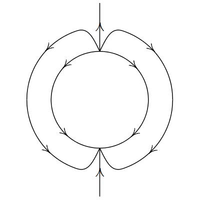
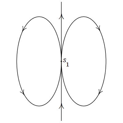
Figure 1: Blow-up and blow-down for $b<1$

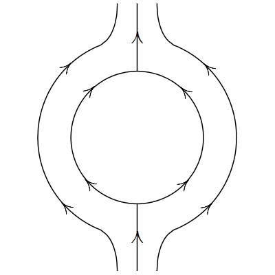
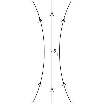
Figure 2: Blow-up and blow-down for $b>1$

We consider now the case $b=1$. In this situation the term $(b-1)x^{2}$ in the second equation of (7) vanishes. This has the effect that, compared to the case $b\neq 0$, the Newton polygon yields different weights $(\alpha,\beta)$ for the quasi-homogeneous directional blow-up, namely $(1,2)$.

First we perform the blow-up in positive $x$-direction. With the above weights, the change of variables for the positive $x$-direction is $(x,y)=(\bar{x},\bar{x}^{2}\bar{y})$. The blown-up vector field is

$$\dot{\bar{x}}\ = \ \bar{x}(\bar{y}-a-a\bar{x}^{2}\bar{y}^{2}),$$

$$\dot{\bar{y}}\ = \ \bar{y}((2a-1)(\bar{x}^{2}\bar{y}^{2}+1)-\bar{y}).$$

We determine its stationary points on $\bar{x}=0$. Clearly the right hand side of the first equation always vanishes on $\bar{x}=0$. Reducing the right hand side of the second equation with $\bar{x}=0$ leaves us with the condition $\bar{y}((2a-1)-\bar{y})=0$ for a stationary point. This last equation is satisfied if and only if $\bar{y}=0$ or $\bar{y}=2a-1$. Thus on $\bar{x}=0$ the stationary points of the system are $(0,0)$ and $(0,2a-1)$. The dynamics in a neighborhood of these points can be read off from the eigenvalues of their linear parts. The Jacobian of the system reduces at these points to $J(0,0)=\mathrm{diag}(-a,2a-1)$ and $J(0,2a-1)=\mathrm{diag}(a-1,1-2a)$.

Obviously, the eigenvalues of these Jacobians depend on the parameter $a>0$. The values of $a$ for which an eigenvalue reduces to zero are clearly $a=1/2$ and $a=1$. Recall that we only consider in this section parameter values such that $s_{1}$ is an isolated stationary point, that is we ignore the case $a=1$. Overall we distinguish between the following cases:

(a)

If $a<1/2$, then the first Jacobian matrix has two negative eigenvalues and the second one has a negative and a positive eigenvalue. We conclude with [Dumortier et al., 2006, Theorem 2.15] that the stationary point $(0,0)$ is an hyperbolic attracting node and that the stationary point $(0,2a-1)$ is a saddle. Note that in the latter case the point lies in the half plane $y\leq 0$. The phase portrait of this blow up is represented graphically in the right half sphere of Figure 4 with corresponding stationary points $p_{1}$ and $p_{2}$.

(b)

If $a=1/2$, then the two stationary points and their Jacobian matrices coincide. One eigenvalue is negative and the other one is zero. So the stationary point $(0,0)$ is semi-hyperbolic. In order to apply [Dumortier et al., 2006, Theorem 2.19] we consider the negative vector field. Then the nonzero eigenvalue is positive and we need to find a solution $x=f(y)$ in a neighbourhood of $(0,0)$ of the equation $\frac{1}{2}x^{3}y^{2}-xy+\frac{1}{2}x=0$ where the notation is as in the theorem. A solution is clearly $x=f(y)=0$ and substituting it into $g(x)=y^{2}$, the theorem implies that the stationary point is a saddle-node. The graphic representation of this blow up is given in the right half plane of Figure 4 where the stationary point is denoted by $p_{1}$.

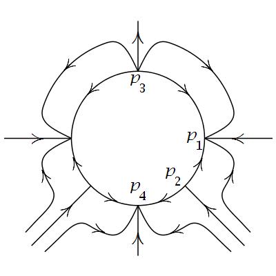
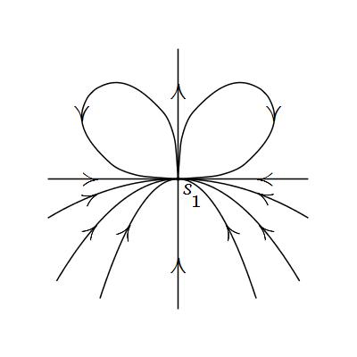
Figure 3: Blow-up and blow-down for $b=1$ and $a<0.5$

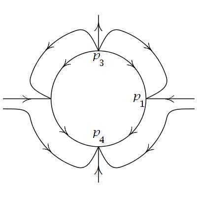
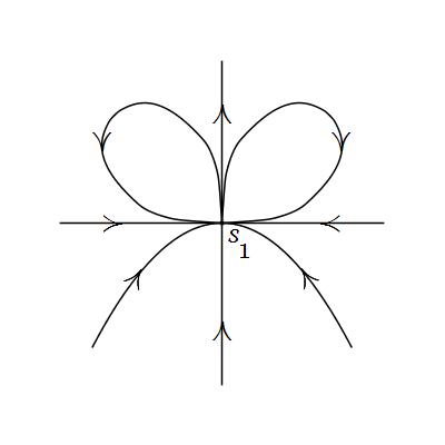
Figure 4: Blow-up and blow-down for $b=1$ and $a=0.5$

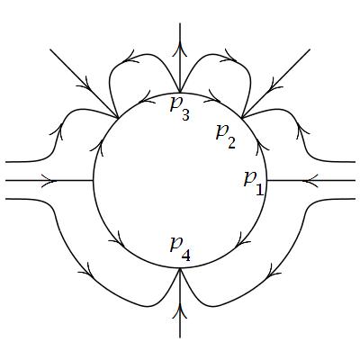
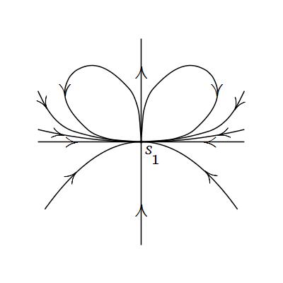
Figure 5: Blow-up and blow-down for $b=1$ and $0.5<a<1$

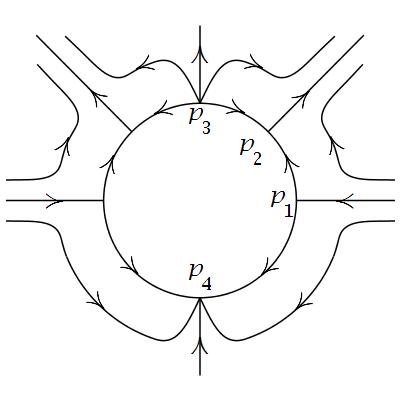
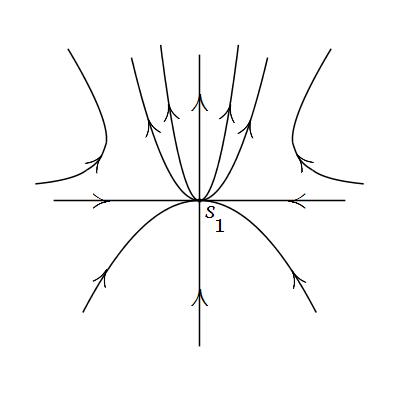
Figure 6: Blow-up and blow-down for $b=1$ and $a>1$

(c)

If $1>a>1/2$, then the two eigenvalues of $J(0,0)$ have opposite sign and the eigenvalues of $J(0,2a-1)$ are both negative, that is, both stationary points are hyperbolic. We conclude with [Dumortier et al., 2006, Theorem 2.15] that $(0,0)$ is a saddle point and that $(0,2a-1)$ is an attracting node. Note that in this case the point $(0,2a-1)$ lies now in the half plane $y\geq 0$. This results of this discussion are represented graphically in the right half plane of Figure 6 where $p_{1}$ and $p_{2}$ stand for $(0,0)$ and $(0,2a-1)$.

(d)

If $a>1$, then the two eigenvalues of both matrices have opposite sign where $J(0,0)$ has a negative and a positive eigenvalue and $J(0,2a-1)$ has a positive and negative eigenvalue. So by [Dumortier et al., 2006, Theorem 2.15] both points are saddle points. In the first case the direction of the $x$-axis is repelling and the direction of the $y$-axis is attracting. In the second case we observe exactly the opposite behaviour. Note that the point $(0,2a-1)$ lies again in the half plane $y\geq 0$. The phase portrait of this blow-up is sketched in the right half plane of Figure 6, where the stationary points are represented by $p_{1}$ and $p_{2}$ correspondingly.

The blow-up in negative $x$-direction yields no new information, since $\alpha$ is odd. According to the same case distinctions, we obtain the same stationary points with the same dynamical behaviour. It is sketched in the left half plane of Figs. 4–6.

For the blow-up in positive $y$-direction with weights $(1,2)$, we use the transformation $(x,y)=(\bar{x}\bar{y},\bar{y}^{2})$ leading to the system

$$\dot{\bar{x}} = -\bar{x}\left((2a-1)(\bar{y}^{2}+\bar{x}^{2})-1\right),$$

$$\dot{\bar{y}} = -\bar{y}(\bar{y}^{2}+\bar{x}^{2}-1).$$

We determine the stationary points of the system on $\bar{y}=0$. Obviously for $\bar{y}=0$ the right hand side of the second equation vanishes and so the condition for a stationary point on $\bar{y}=0$ is given by $\bar{x}((2a-1)\bar{x}^{2}-1)=0$. We conclude that the stationary points on $\bar{y}=0$ are $(0,0)$ and $(\pm 1/\sqrt{2a-1},0)$. The latter two points are real only for $a>\frac{1}{2}$ and we already analysed these two points in the blow-up in positive $x$-direction in the respective case. So it is left to determine the qualitative behaviour near $(0,0)$. It is easily checked that the Jacobian reduces at $\bar{x}=0$ and $\bar{y}=0$ to the unit matrix. This means that independent of the parameter values we have two positive eigenvalues and so by [Dumortier et al., 2006, Theorem 2.15] the stationary point is a repelling node. The results of this discussion are represented graphically in the upper half plane of Figs. 4–6 where the stationary point is denoted by $p_{3}$.

For the blow-up in negative $y$-direction with the same weights we use $(x,y)=(\bar{x}\bar{y},-\bar{y}^{2})$ and obtain

$$\dot{\bar{x}} = -\bar{x}\left((2a-1)(\bar{y}^{2}+\bar{x}^{2})+1\right),$$

$$\dot{\bar{y}} = -\bar{y}(\bar{y}^{2}+\bar{x}^{2}+1).$$

Similar as above, we conclude that the condition for a stationary point of the system on $\bar{y}=0$ is given by the equation $\bar{x}((2a-1)\bar{x}^{2}+1)=0$. Clearly $(0,0)$ is a stationary point independent of the parameter value $a>0$. For $a<\frac{1}{2}$ the coefficient $(2a-1)$ is negative and so there are two additional real stationary points, namely $(\pm 1/\sqrt{-(2a-1)}),0)$. The dynamics of these two points have already been discussed in the blow-ups in positive and negative $x$-direction. So we only need to analyse the dynamics near $(0,0)$. It is easily checked that the Jacobian reduces at $(\bar{x},\bar{y})=(0,0)$ to the negative of the unit matrix and so the stationary point $(0,0)$ is an attracting node by [Dumortier et al., 2006, Theorem 2.15]. In Figs. 4–6, this point is called $p_{4}$.

Lemma 4.3.

Assume we are in case (2) or (3) of Lemma 4.1. Then at the isolated stationary point $s_{1}$ we have the following dynamical behaviour:

1. For $b<1$ there are two elliptic sectors as in Fig. 2.

2. For $b>1$ there are two parabolic sectors as in Fig. 2.

3. For $b=1$ there are four subcases:

   1. For $a<1/2$ there are two elliptic sectors in the upper half plane and four hyperbolic sectors in the lower half plane as in Fig. 4.

   2. For $a=1/2$ there are two elliptic sectors in the upper half plane and two hyperbolic sectors in the lower half plane as in Fig. 4.

   3. For $1>a>1/2$ there are in the upper half plane two elliptic and two hyperbolic sectors and two additional hyperbolic sectors in the lower half plane as in Fig. 6.

   4. For $a>1$ there are in the upper half plane two parabolic and two hyperbolic sectors and two additional hyperbolic sectors in the lower half plane as in Fig. 6.

4.4 The Dynamics at the Stationary Points $s_{3}$ and $s_{4}$

In this section we determine the dynamics near the stationary points $s_{3}$ and $s_{4}$. Recall that, according to Lemma 4.1, these points are stationary if and only if the parameters $a$, $b>0$ satisfy either $b>1>a$ or $a>1>b$. Therefore we assume throughout this section that $a$ and $b$ are chosen such that one of these relations is fulfilled.

In order to apply the standard results of Dumortier et al. [2006], we need to move each of the stationary points $s_{3}$ and $s_{4}$ with a correspond change of variables to the origin. By Lemma 4.1, the stationary points are $s_{3}=(x_{1},y_{2})$ and $s_{4}=(x_{2},y_{2})$. Thus the transformation $(x,y)=(x_{k}+\bar{x},y_{2}+\bar{y})$ moves for $k=1$ the point $s_{3}$ and for $k=2$ the point $s_{4}$ to the origin. Applying this transformation to the original system, we obtain the new system

$$\dot{\bar{x}} = -((\bar{x}^{2}+2x_{k}\bar{x}+\bar{y}^{2}+2y_{2}\bar{y}+x_{k}^{2}+y_{2}^{2})a-\bar{y}-y_{2})(\bar{x}+x_{k}),$$

$$\dot{\bar{y}} = -(\bar{y}+y_{2}-1)(\bar{x}^{2}+2x_{k}\bar{x}+\bar{y}^{2}+2y_{2}\bar{y}+x_{k}^{2}+y_{2}^{2})b-(\bar{x}+x_{k})^{2},$$

which depends obviously on the values for $x_{k}$ and $y_{2}$. In order to determine its dynamical behaviour near the origin, we compute the eigenvalues of its linear part. If we reduce the entries of the Jacobian matrix with $y_{2}=-(b-1)/(a-b)$ and $(\bar{x},\bar{y})=(0,0)$, we get the matrix

$$J(0,0)=\begin{pmatrix}\frac{2b(b-1)(a-1)}{(a-b)^{2}}&\frac{((2b-1)a-b)x_{k}}{a-b}\\ \frac{2a(b-1)x_{k}}{a-b}&-\frac{b(b-1)(2a^{2}-3a+b)}{a(a-b)^{2}}\end{pmatrix}$$

whose entries depend on the value for $x_{k}$. The eigenvalues of $J(0,0)$ compute as

$$\lambda_{1/2}=\frac{b(1-b)\pm(b-1)\sqrt{b(b+8a(a-1))}}{2a(b-a)}\,.$$

We see that they do not depend on $x_{k}$ and so the dynamics near the stationary points $s_{3}$ and $s_{4}$ of the original system are qualitatively the same. For its determination it is useful to make the following case distinctions for the parameters $a$ and $b$:

(a)

Suppose that $b>1>a$. It follows that the expression $8a(a-1)$ is a negative real number. If we assume in addition that $|8a(a-1)|>b$, then the imaginary parts of the eigenvalues $\lambda_{1/2}$ are nonzero and $\lambda_{1/2}$ are complex conjugated to each other. Further from $b>1$ and $b>a$ it follows that their common real part is negative. By [Dumortier et al., 2006, Theorem 2.15 (iii)] the origin is in this situation a strong attracting focus. Now suppose that $|8a(a-1)|\leq b$. Then both eigenvalues are real and in order to determine the dynamics we need to decide whether they are positive or negative. It follows from the assumption that $2a(b-a)$ is positive and so $b(1-b)/(2a(b-a))$ is negative. Because $b-1$ and $\sqrt{b(b+8a(a-1))}$ are both positive, the second summand in the expression for the eigenvalues is also positive. We conclude that the eigenvalue $\lambda_{2}$ is negative. The eigenvalue $\lambda_{1}$ is also negative. Indeed, the inequation $8a(a-1)<0$ implies that $\sqrt{b(b+8a(a-1))}<b$ and so we have $b(1-b)+(b-1)\sqrt{b(b+8a(a-1))}<0$. Because both eigenvalues are real and negative we obtain from [Dumortier et al., 2006, Theorem 2.15 (ii)] that the stationary point is an attracting node.

(b)

Assume that $a>1>b$. It is easily seen that then the eigenvalues are real numbers and we need to determine if they are positive are negative. The real numbers $2a(b-a)$ and $b-1$ are clearly negative and the product $b(1-b)$ is positive. We conclude that $b(1-b)/(2a(b-a))<0$ and $(b-1)/(2a(b-a))>0$. It can be easily checked now that $\lambda_{2}$ is negative. Further the inequation $8a(a-1)>0$ implies that $\sqrt{b(b+8a(a-1))}>b$ and so $b(1-b)+(b-1)\sqrt{b(b+8a(a-1))}<0$, because $(b-1)$ is negative. We conclude that $\lambda_{1}$ is positive. It follows from [Dumortier et al., 2006, Theorem 2.15 (i)] that the stationary point is a saddle point.

Lemma 4.4.

In the situation of Lemma 4.1 (2), we have the following dynamical behaviour at the stationary points $s_{3}$ and $s_{4}$:

1. For $b>1>a$ and $|8a(a-1)|>b$ each point is a strong attracting focus.

2. For $b>1>a$ and $|8a(a-1)|\leq b$ each point is an attracting node.

3. For $a>1>b$ each point is a saddle point.

4.5 The Infinite Stationary Points

In this section we determine the local phase portrait at the infinite stationary points using the Poincaré compactification. The basic idea of the Poincaré compactification is a specific projection of a given planar vector field to the northern and southern hemisphere of the unit sphere and to extend this vector field to the equator. The dynamics at the points of the equator represent then the dynamics at the infinite points of the planar system. The construction of the Poincaré compactification can be found in [Dumortier et al., 2006, Section 5.1 & 5.2]. Throughout this section we use the notation and the formulas given there. Our computations are done in the charts $(U_{1},\phi_{1})$ and $(U_{2},\phi_{2})$ representing the front and right hemisphere and the charts $(V_{1},\psi_{1})$ and $(V_{2},\psi_{2})$ covering the back and left hemisphere.

Obviously, the maximal degree of the polynomial right hand sides $P$ and $Q$ of the system (7) is three and we can write them as the sums of homogeneous polynomials $P=P_{2}+P_{3}$ and $Q=Q_{2}+Q_{3}$ with $P_{2}=xy$, $P_{3}=-a(x^{3}+xy^{2})$, $Q_{2}=by^{2}+(b-1)x^{2}$ and $Q_{3}=-b(y^{3}+yx^{2})$. Substituting the homogeneous polynomials $P_{3}$ and $Q_{3}$ in the corresponding formula, we obtain that a point $(u,0)$ of $\mathbb{S}^{1}\cap(U_{1}\cup V_{1})$ is stationary if and only if

$$F(u)=-b(u^{3}+u)-u(-a(1+u^{2}))=(a-b)u(u^{2}+1)=0.$$

We conclude that for $a\neq b$ we have exactly one real stationary point on the $u$-axis, namely $(u,0)=(0,0)$. By contrast, for $a=b$ every point on the $u$-axis is stationary. Moreover, a point $(u,0)$ of $\mathbb{S}^{1}\cap(U_{2}\cup V_{2})$ is stationary if and only if

$$G(u)=a(u^{3}+u)-u(-b(1+u^{2}))=(b-a)u(u^{2}+1)=0.$$

As above for $a\neq b$ the only real stationary point on the $u$-axis is $(u,0)=(0,0)$ and in case $a=b$ every point there is stationary. We determine the dynamics near the isolated stationary point $(u,0)=(0,0)$ in the different charts. Substituting the above homogeneous polynomials as well as $F^{\prime}(u)$ and $G^{\prime}(u)$ in the formulas for the Jacobians we obtain the matrices

$$\begin{pmatrix}a-b&b-1\\ 0&a\end{pmatrix}\qquad\text{resp.}\qquad\begin{pmatrix}b-a&0\\ 0&b\end{pmatrix}$$

which represent the cases if $(0,0)$ belongs to $U_{1}\cup V_{1}$ or $U_{2}\cup V_{2}$, respectively. Because of $a\neq b$, the stationary point $(0,0)$ is in both cases a hyperbolic. In case of the charts $(U_{1},\phi_{1})$ and $(V_{1},\psi_{1})$, it is for $b>a$ a saddle point and for $a>b$ a repelling node by [Dumortier et al., 2006, Theorem 2.15]. In the charts $(U_{2},\phi_{2})$ and $(V_{2},\psi_{2})$ we obtain by the same theorem that it is for $b>a$ a repelling node and for $a>b$ a saddle.

As mentioned above, for $a=b$ every point on the $u$-axis in either chart is stationary and we obtain for the corresponding Jacobians

$$\begin{pmatrix}0&(b-1)(u^{2}+1)\\ 0&b(u^{2}+1)\end{pmatrix}\qquad\text{resp.}\qquad\begin{pmatrix}0&(1-b)u(u^{2}+1)\\ 0&b(u^{2}+1)\end{pmatrix}$$

for points on $U_{1}\cup V_{1}$ or $U_{2}\cup V_{2}$, respectively. Obviously, the centre manifold is given by the complete $u$-axis, as it consists of stationary points, and is therefore uniquely determined by [Sijbrand, 1985, Cor. 3.3]. Furthermore, in both cases the second eigenvalue is positive and thus a unique one-dimensional unstable manifold exists [Guckenheimer & Holmes, 1990, Thm. 3.2.1]. This implies that in this case no trajectory can have an $\omega$-limit point at infinity, but that each point there is the $\alpha$-limit point of a unique trajectory, namely its unstable manifold.

Lemma 4.5.

1. If $a=b$, then every point at infinity is a stationary point with one outgoing trajectory.

2. If $a\neq b$, then the points at infinity in positive and negative $x$- and $y$-direction are stationary points.

   1. If $b>a$, then the stationary points at infinity in positive and negative $x$-direction are saddle points and the stationary points at infinity in positive and negative $y$-direction are repelling nodes.

   2. If $a>b$, then the stationary points at infinity in positive and negative $x$-direction are repelling nodes and the stationary points at infinity in positive and negative $y$-direction are saddle points.

4.6 Putting Everything Together

Finally, we collect all our results. As discussed in more detail in the next section, we show for each arising case a phase portrait in the appendix.

Theorem 4.6.

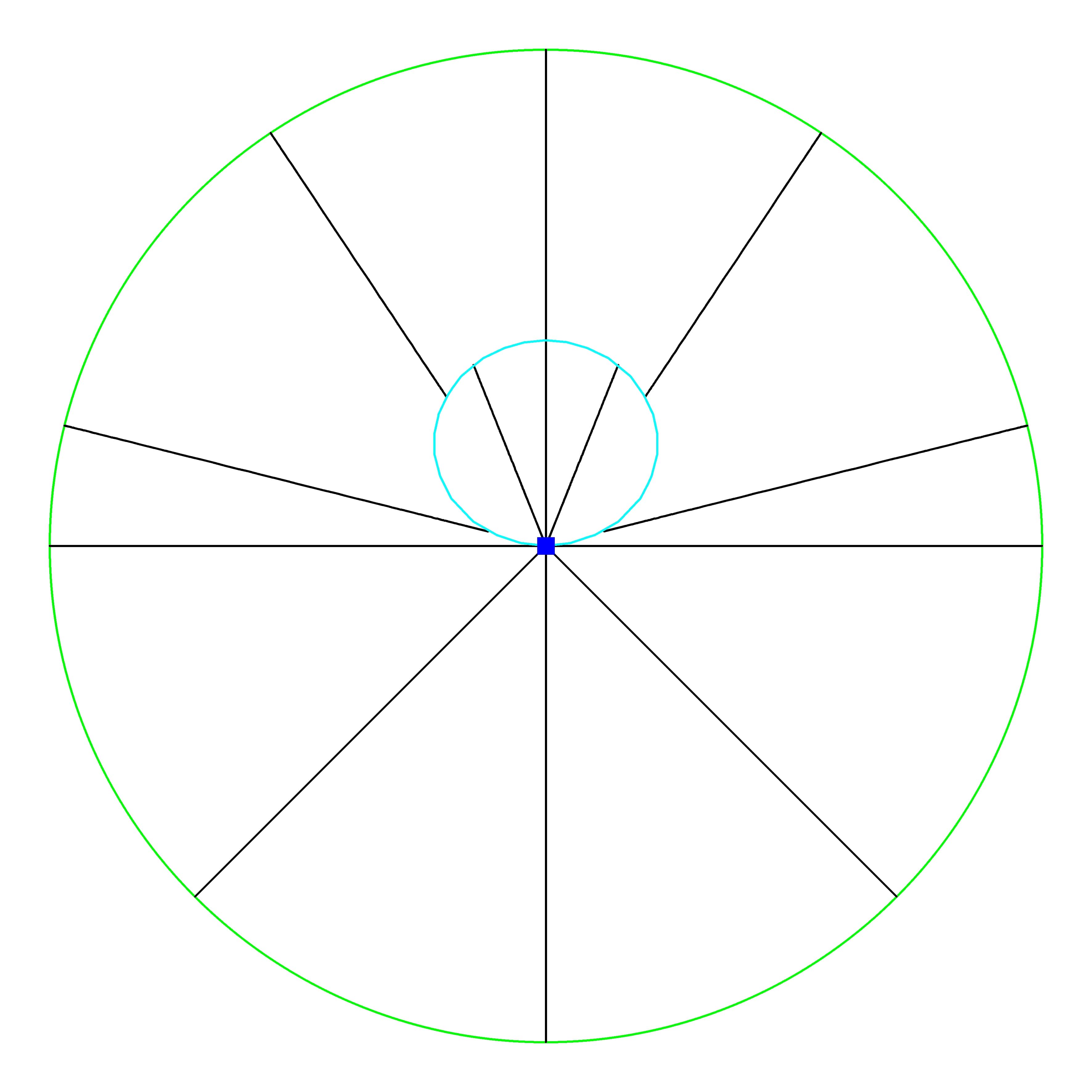
(a)  $a=1.0,\ b=1.0$

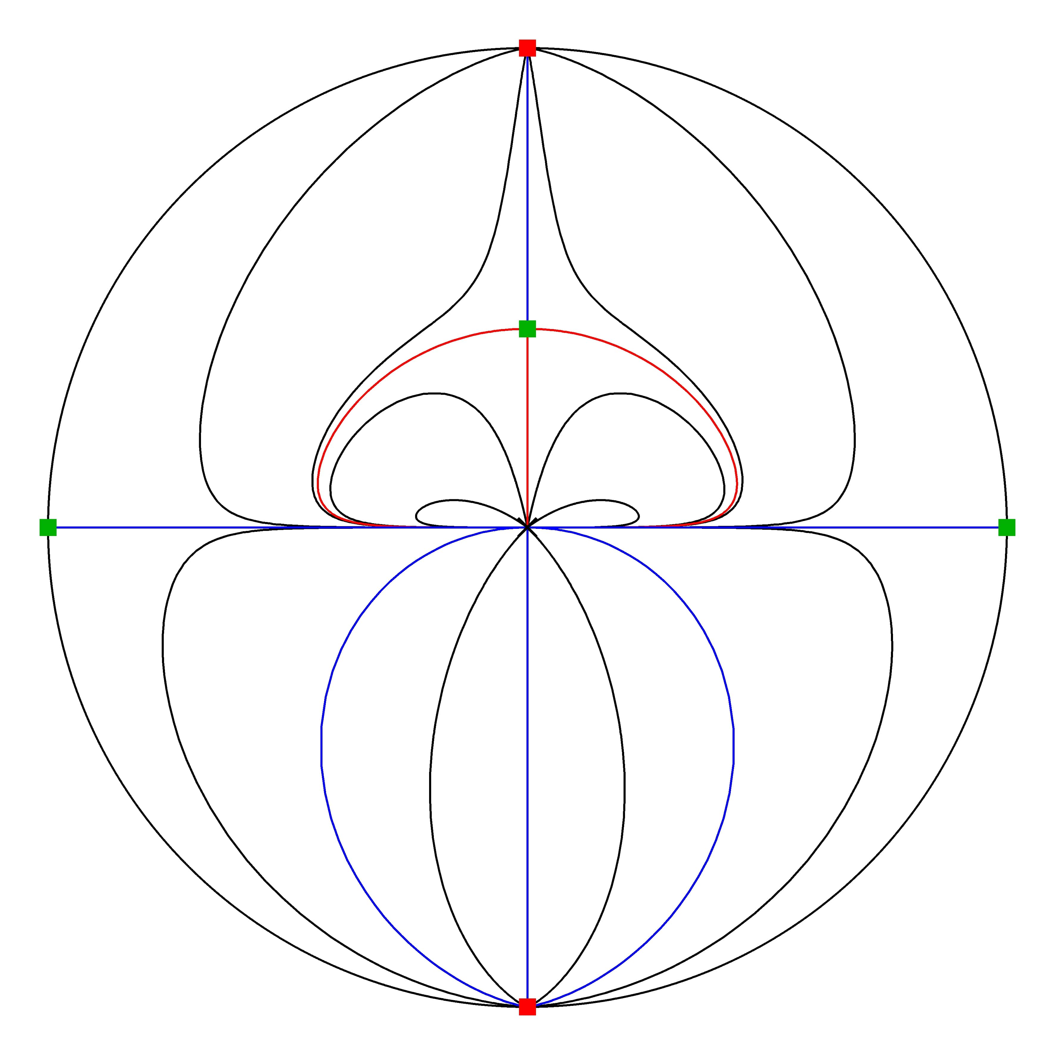
(b)  $a=0.2,\ b=1.0$

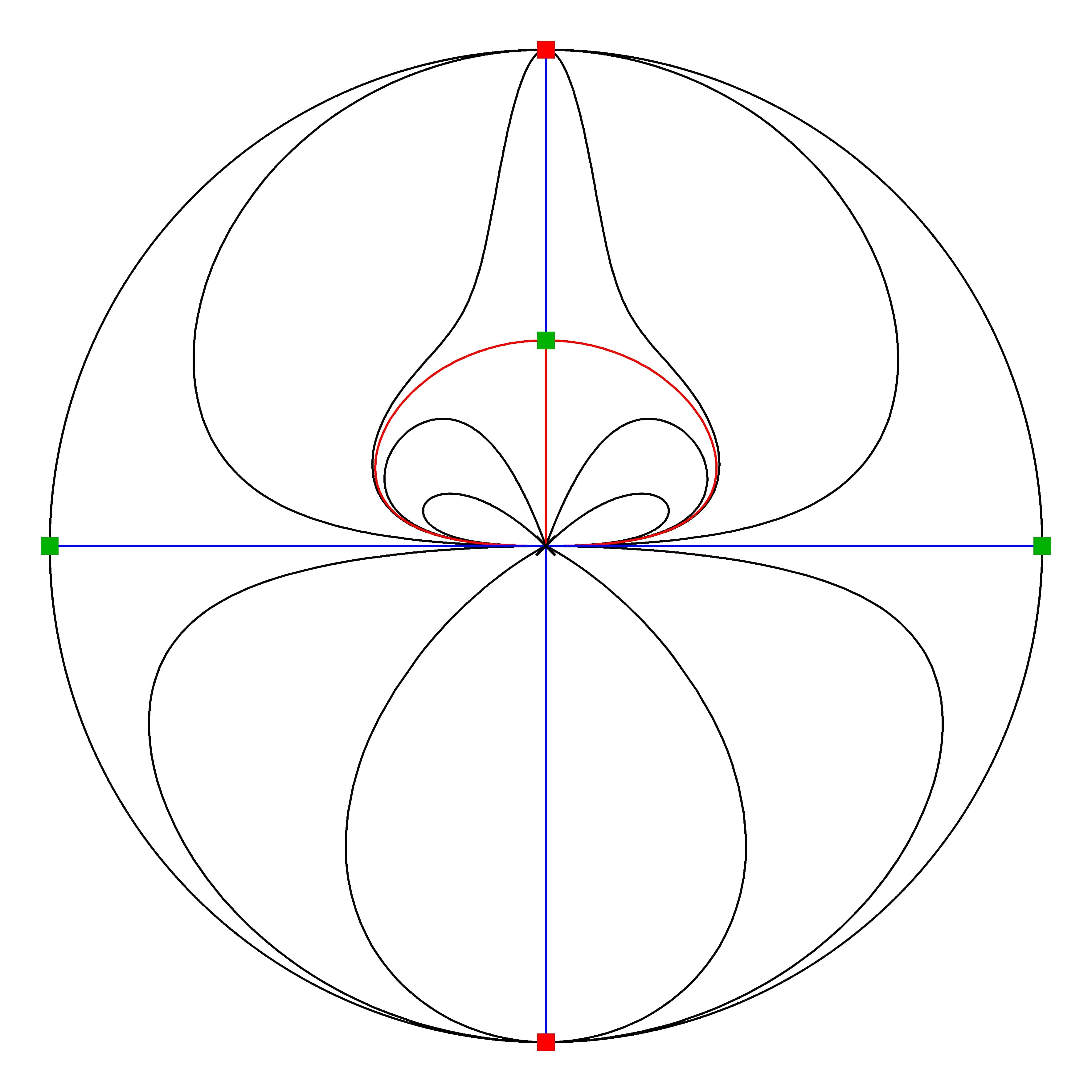
(c)  $a=0.5,\ b=1.0$

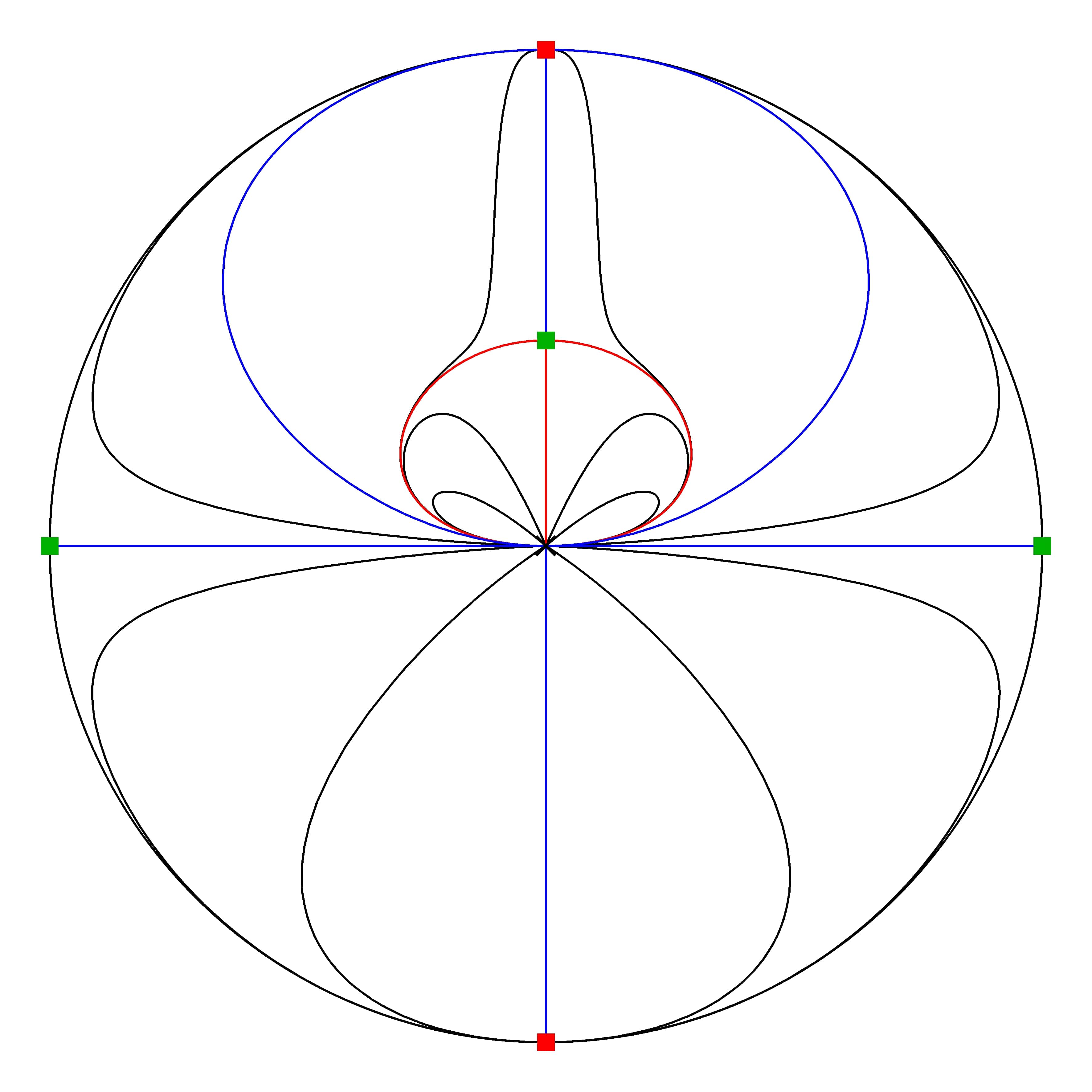
(d)  $a=0.7,\ b=1.0$

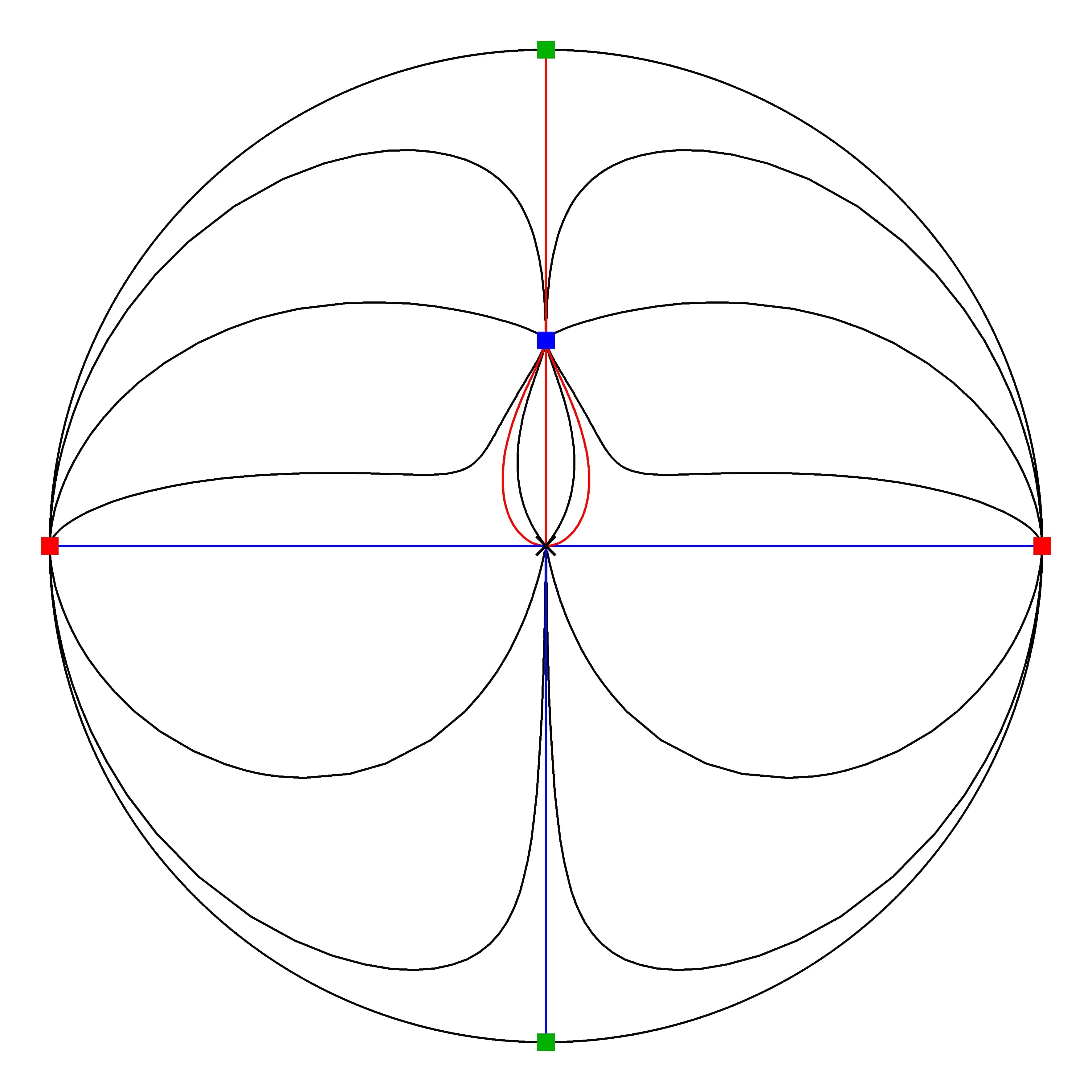
(e)  $a=2.5,\ b=1.0$

Figure 10: Phase portraits of the CDK system for $b=1$ and different values of $a$

1. The dynamics of the system (7) for the parameter values $a=b=1$ is as follows: The finite stationary points are the points on the circle $x^{2}+(y-\tfrac{1}{2})^{2}=\tfrac{1}{4}$. At infinity, every point is a stationary point. The orbits are straight lines starting at infinity in direction to the origin (see Fig. 10(a)).

2. The dynamics of the system (7) for the parameter values as in (2) of Lemma 4.1 is:

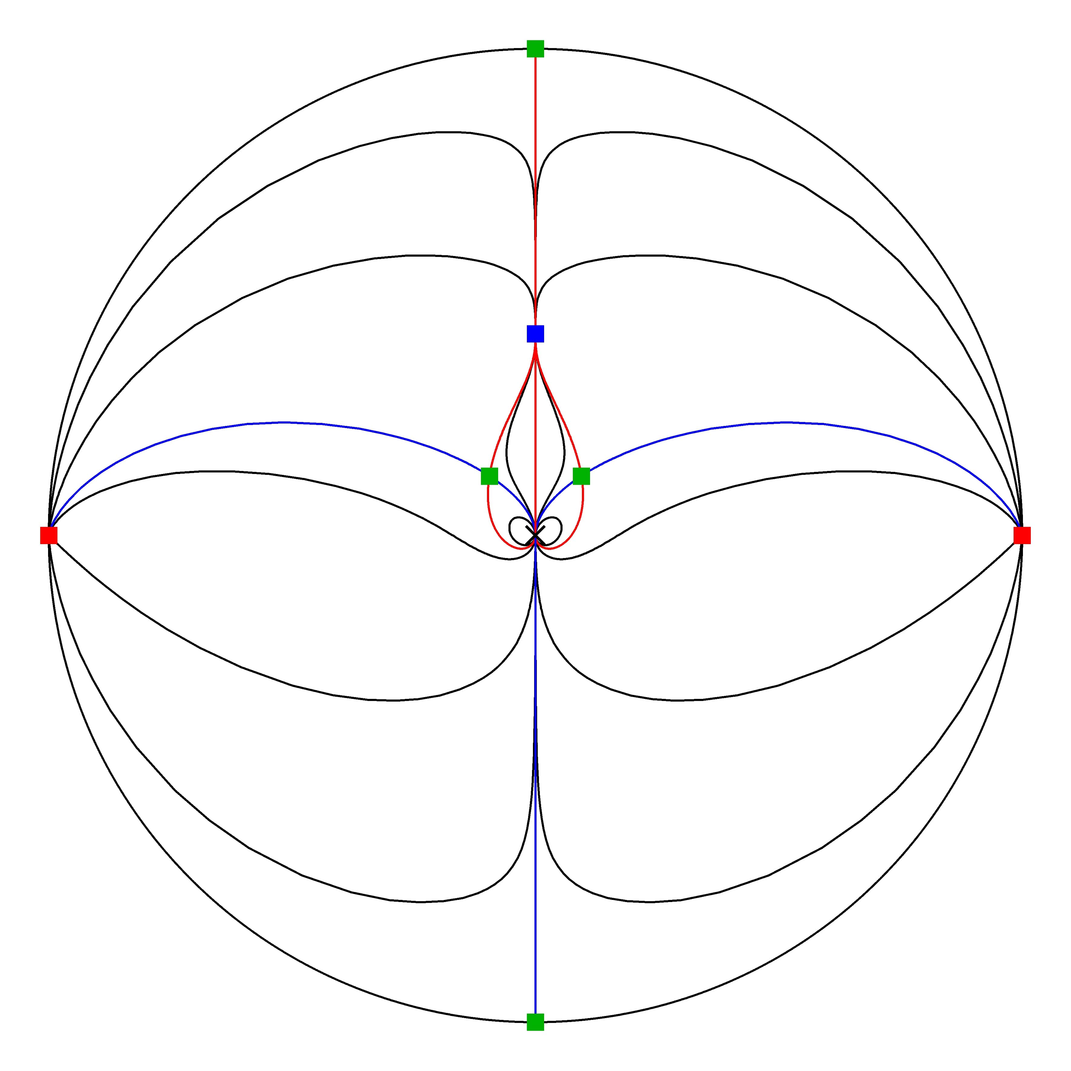
(a)  $a=2.5,\ b=0.5$

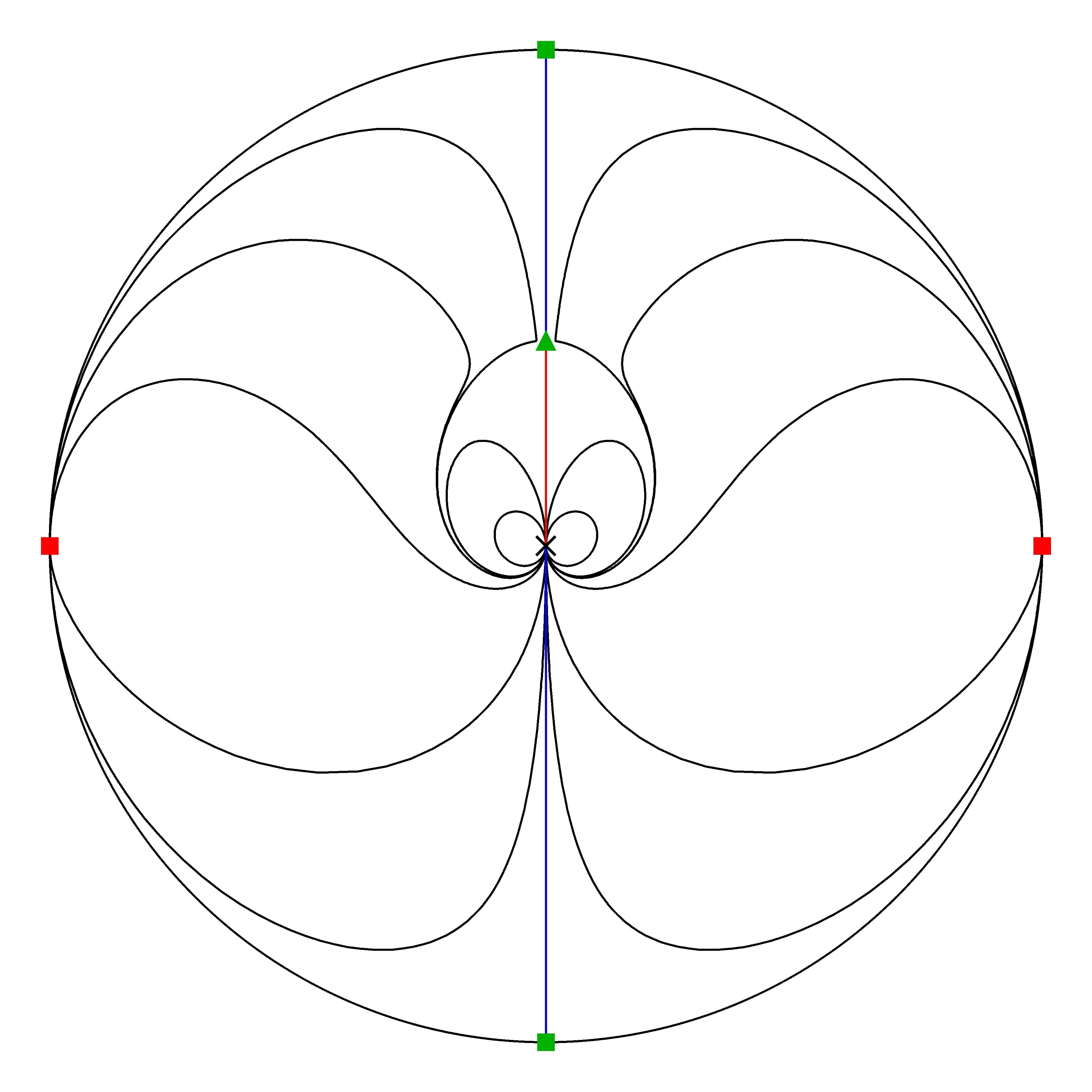
(b)  $a=1.0,\ b=0.5$

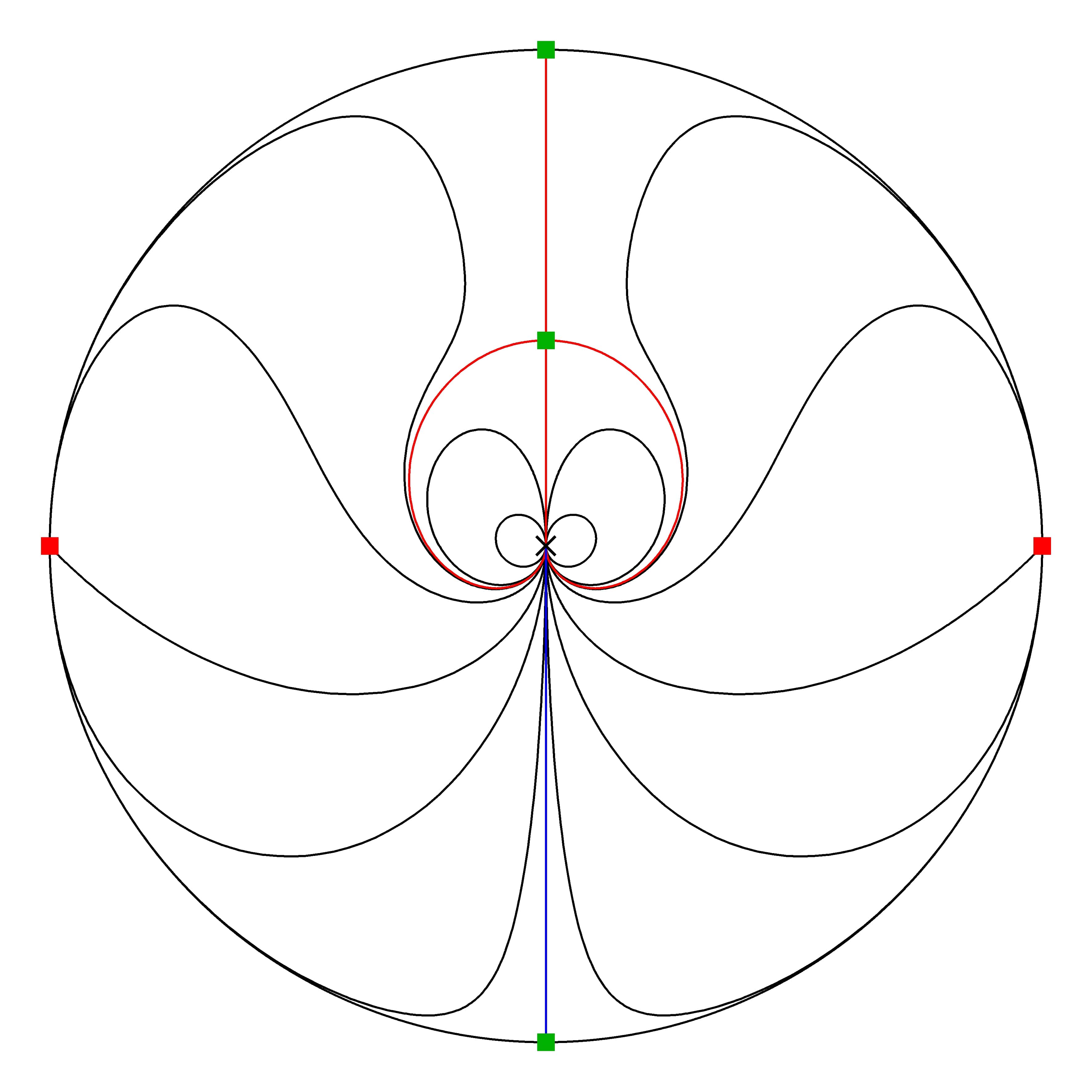
(c)  $a=0.7,\ b=0.5$

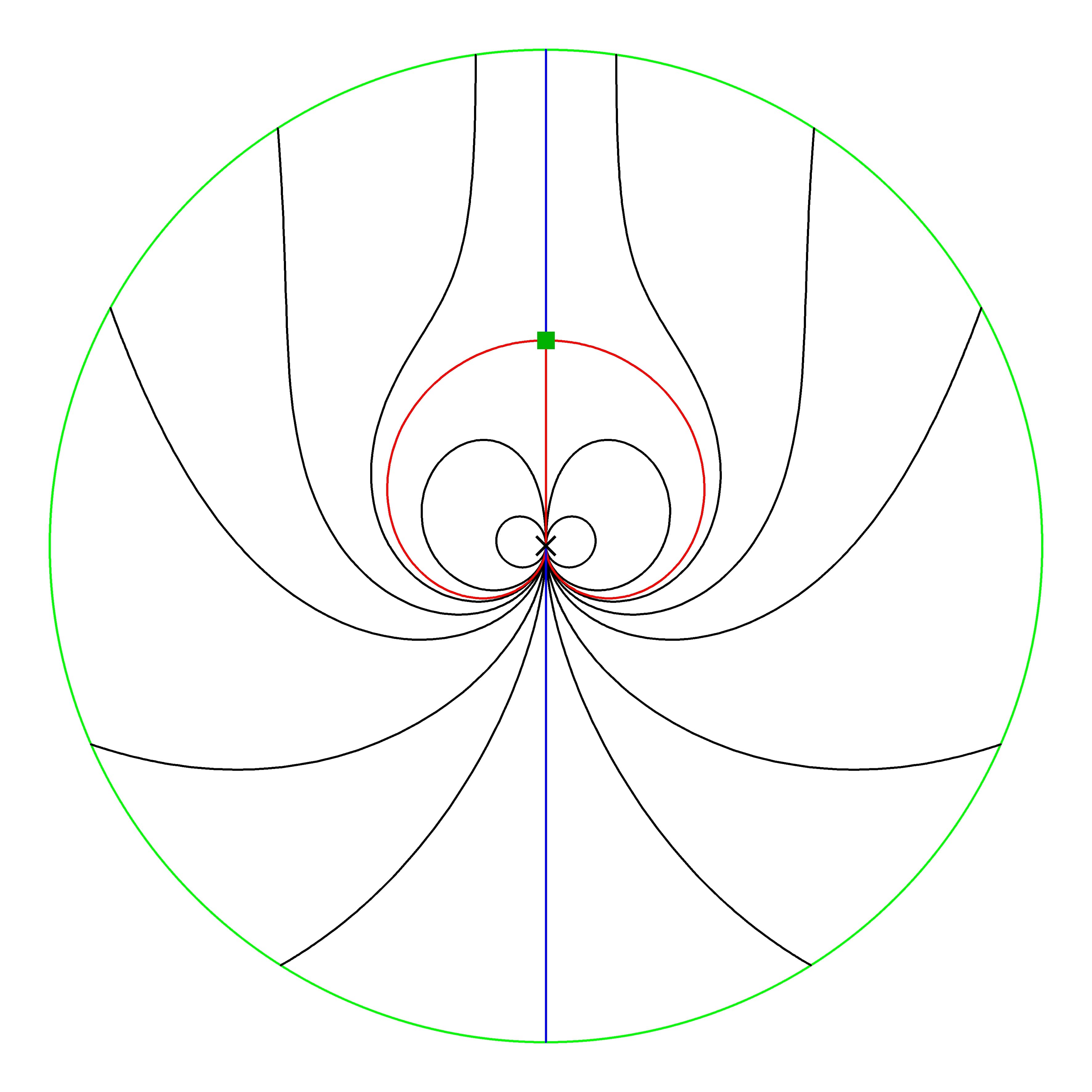
(d)  $a=0.5,\ b=0.5$

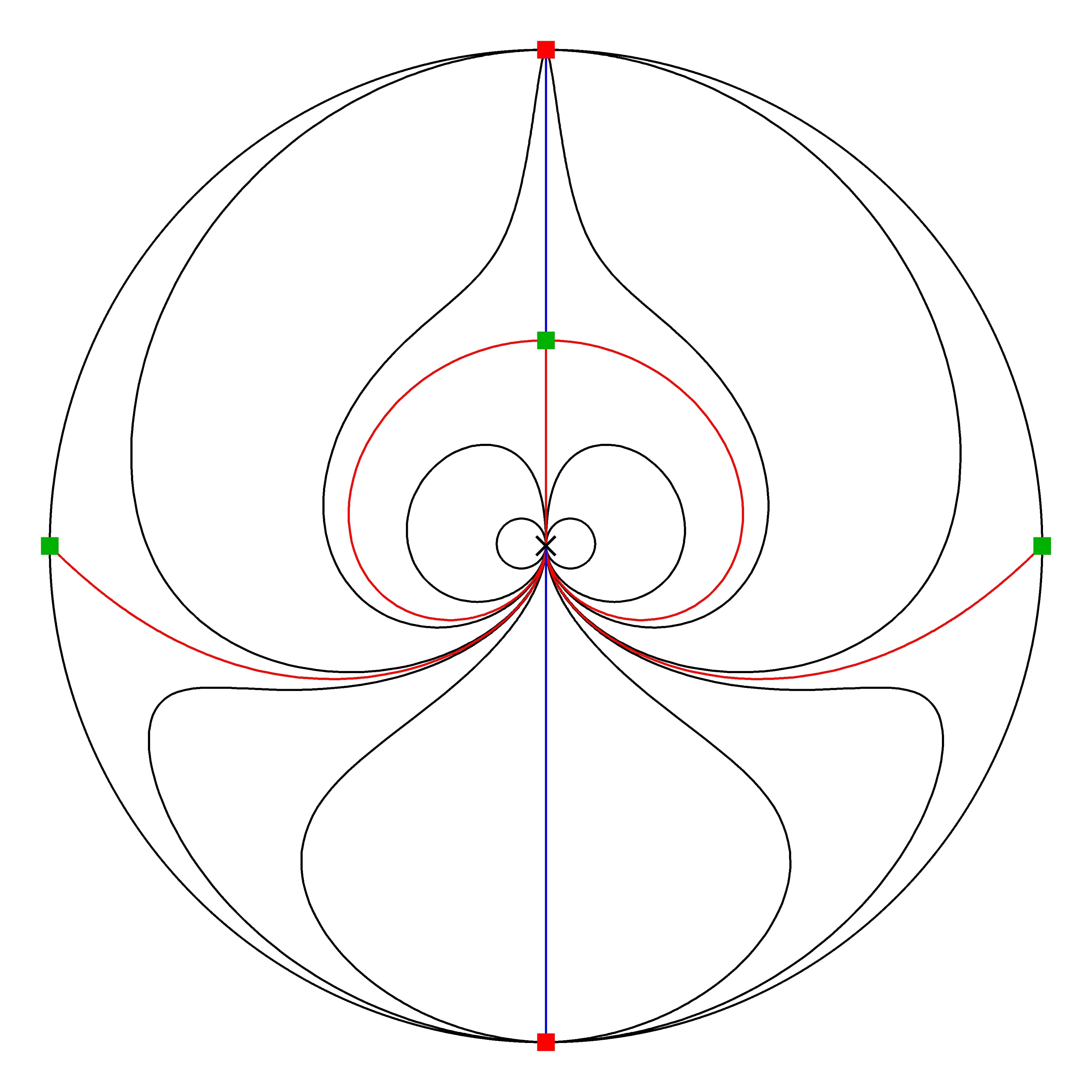
(e)  $a=0.2,\ b=0.5$

Figure 9: Phase portraits of the CDK system for $b=0.5$ and different values of $a$

   1. For $b<1<a$ the stationary point $s_{1}$ has dynamics as in (1) of Lemma 4.3 and the stationary point $s_{2}$ is an attracting node. The points $s_{3}$ and $s_{4}$ are saddle points. The points at infinity in positive and negative $x$-direction are repelling nodes and the ones in positive and negative $y$-direction are saddle points (see Fig. 9(a)).

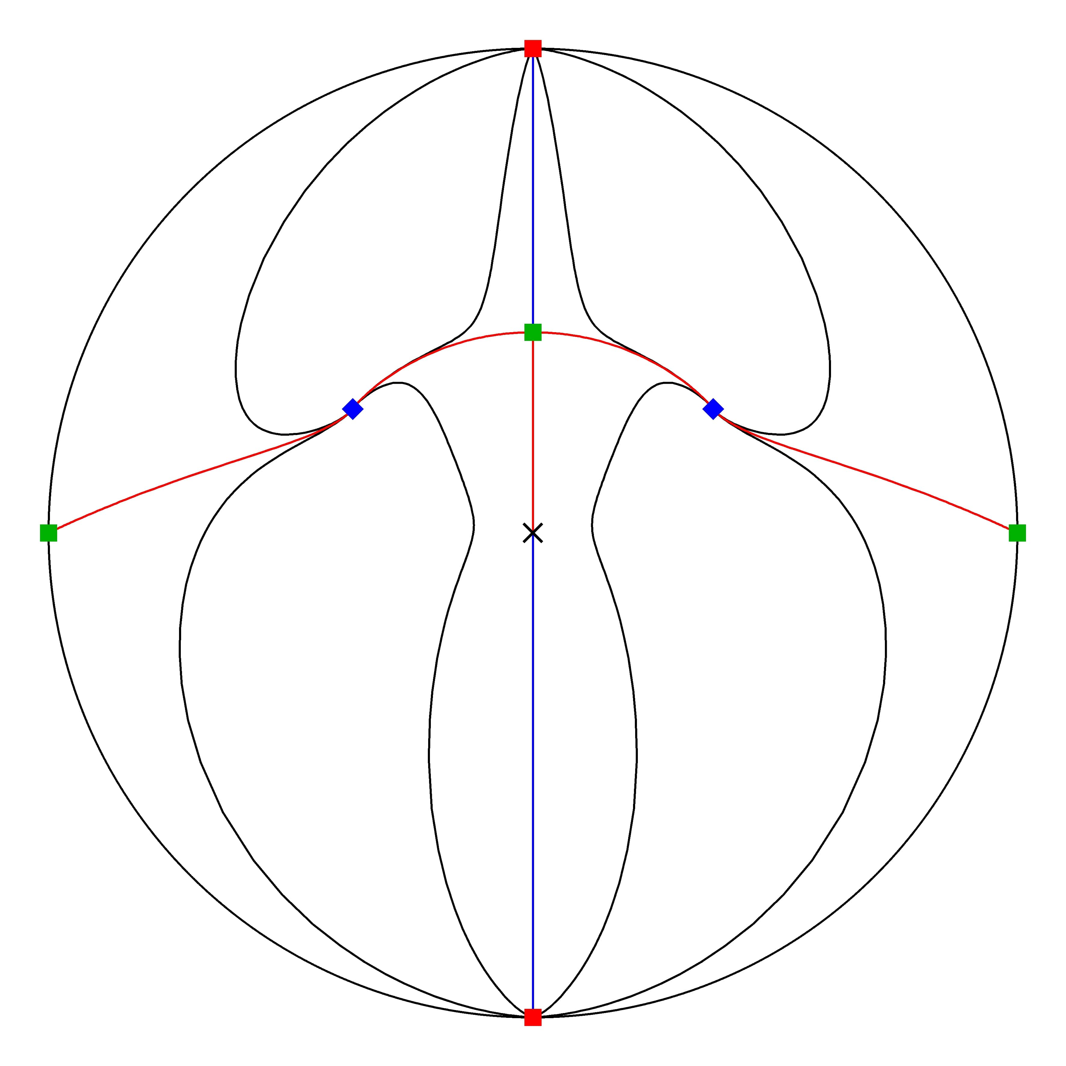
(a)  $a=0.5,\ b=1.9$

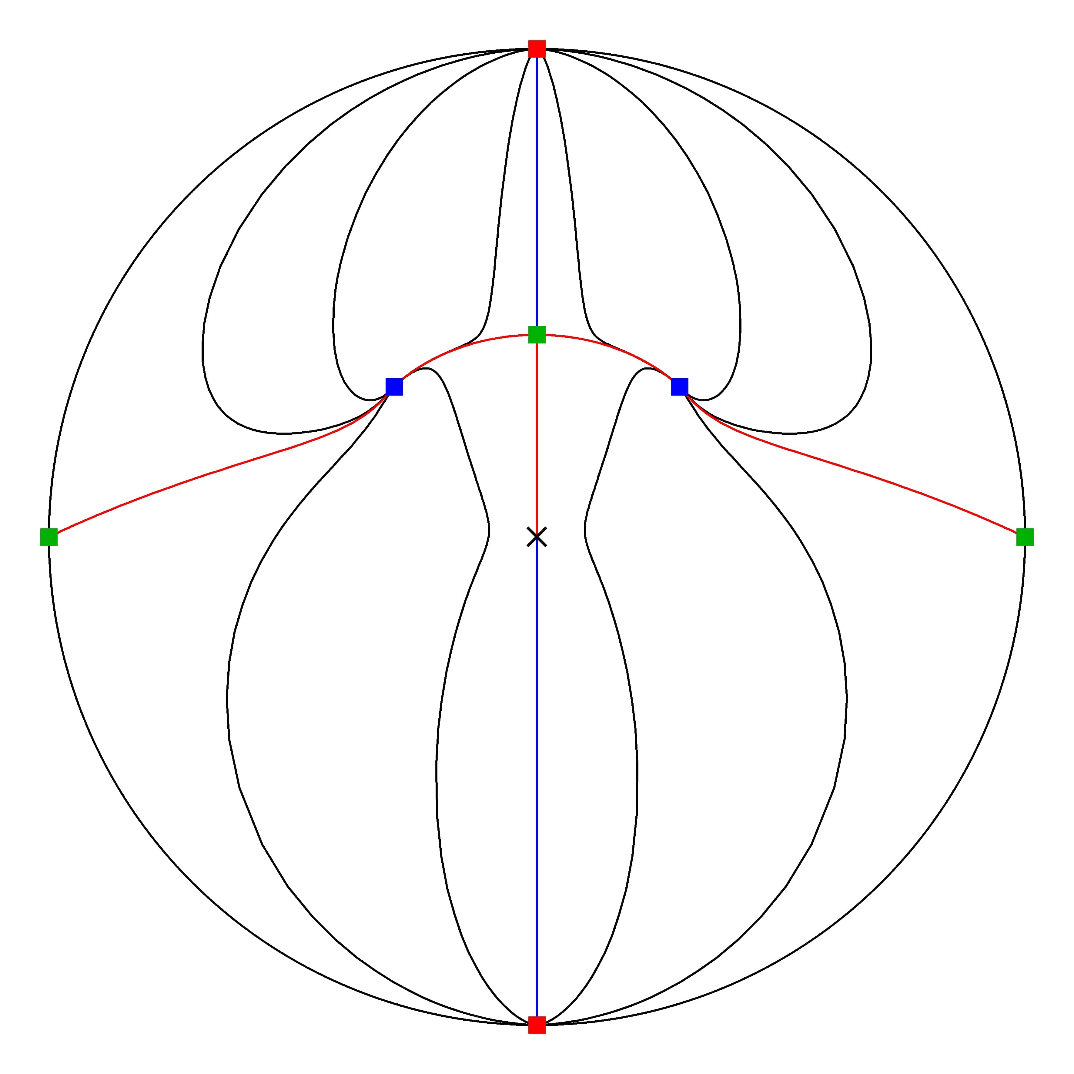
(b)  $a=0.7,\ b=1.9$

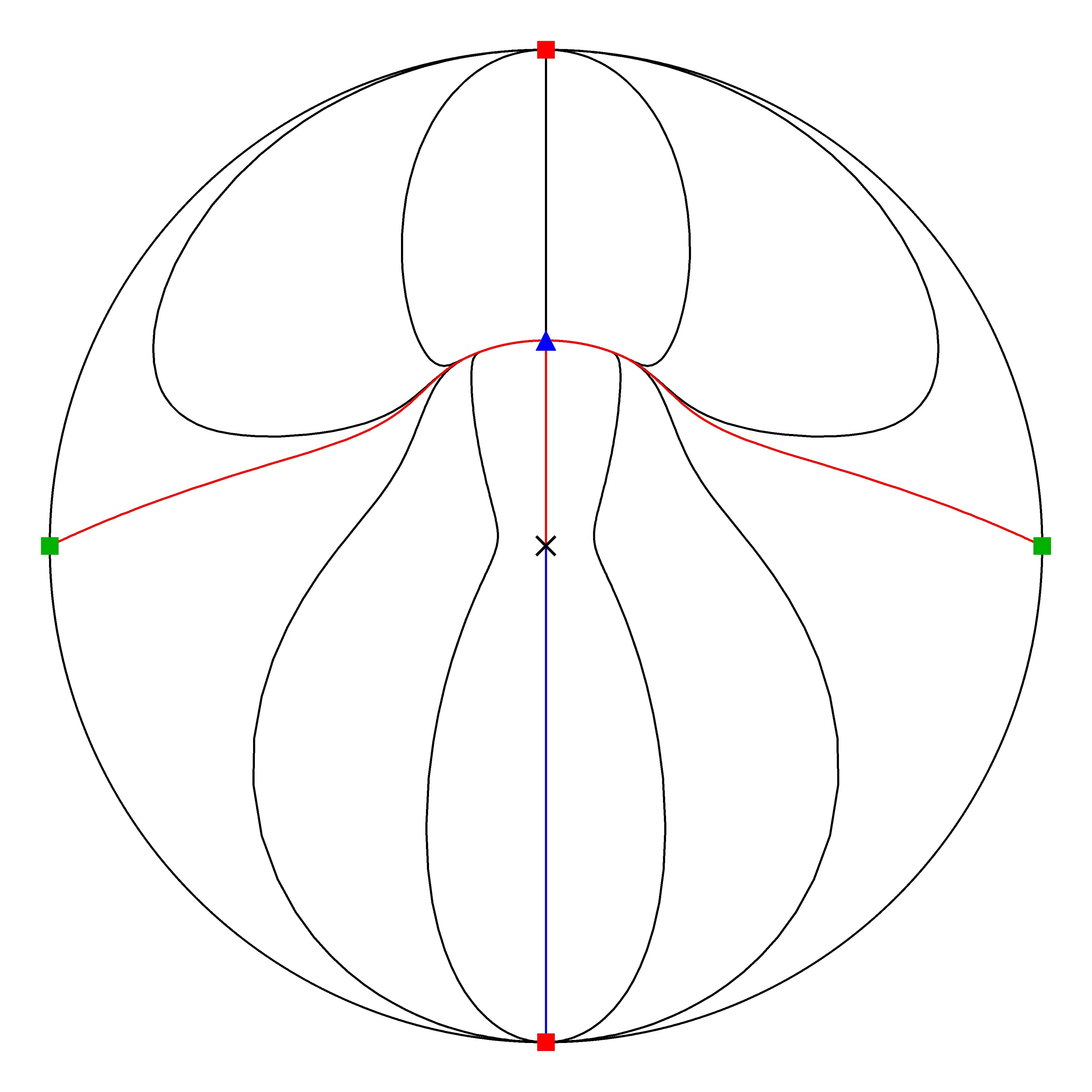
(c)  $a=1.0,\ b=1.9$

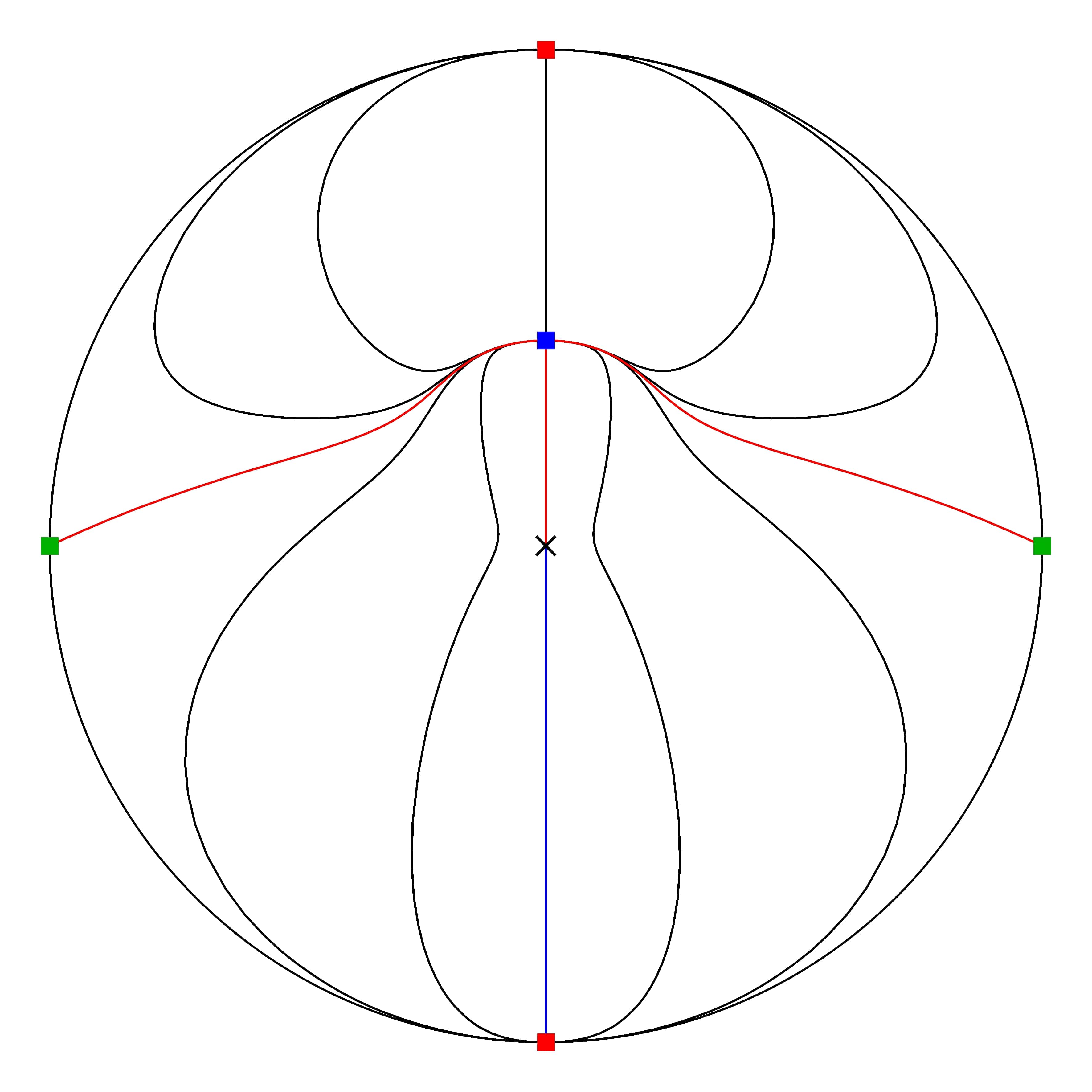
(d)  $a=1.2,\ b=1.9$

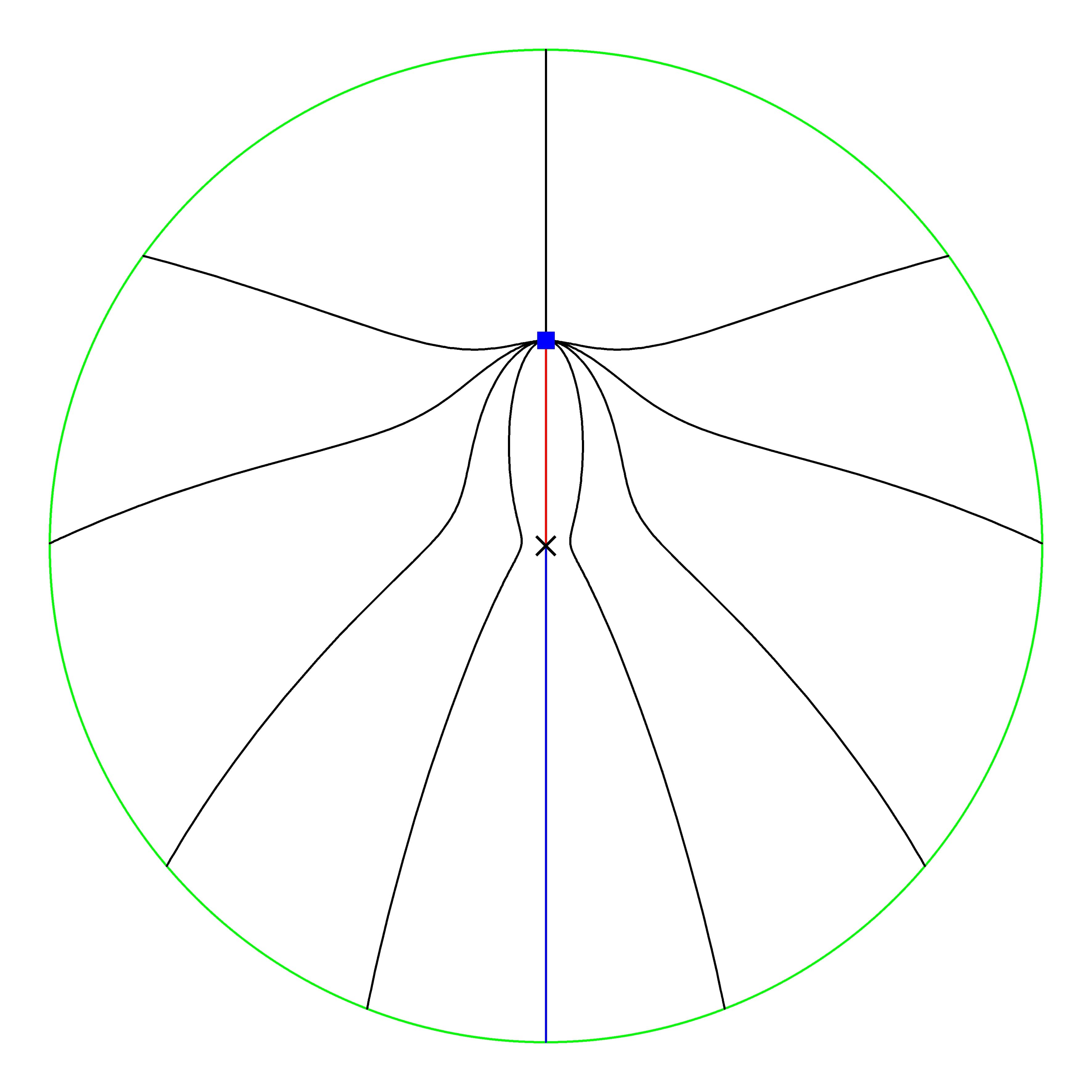
(e)  $a=1.9,\ b=1.9$

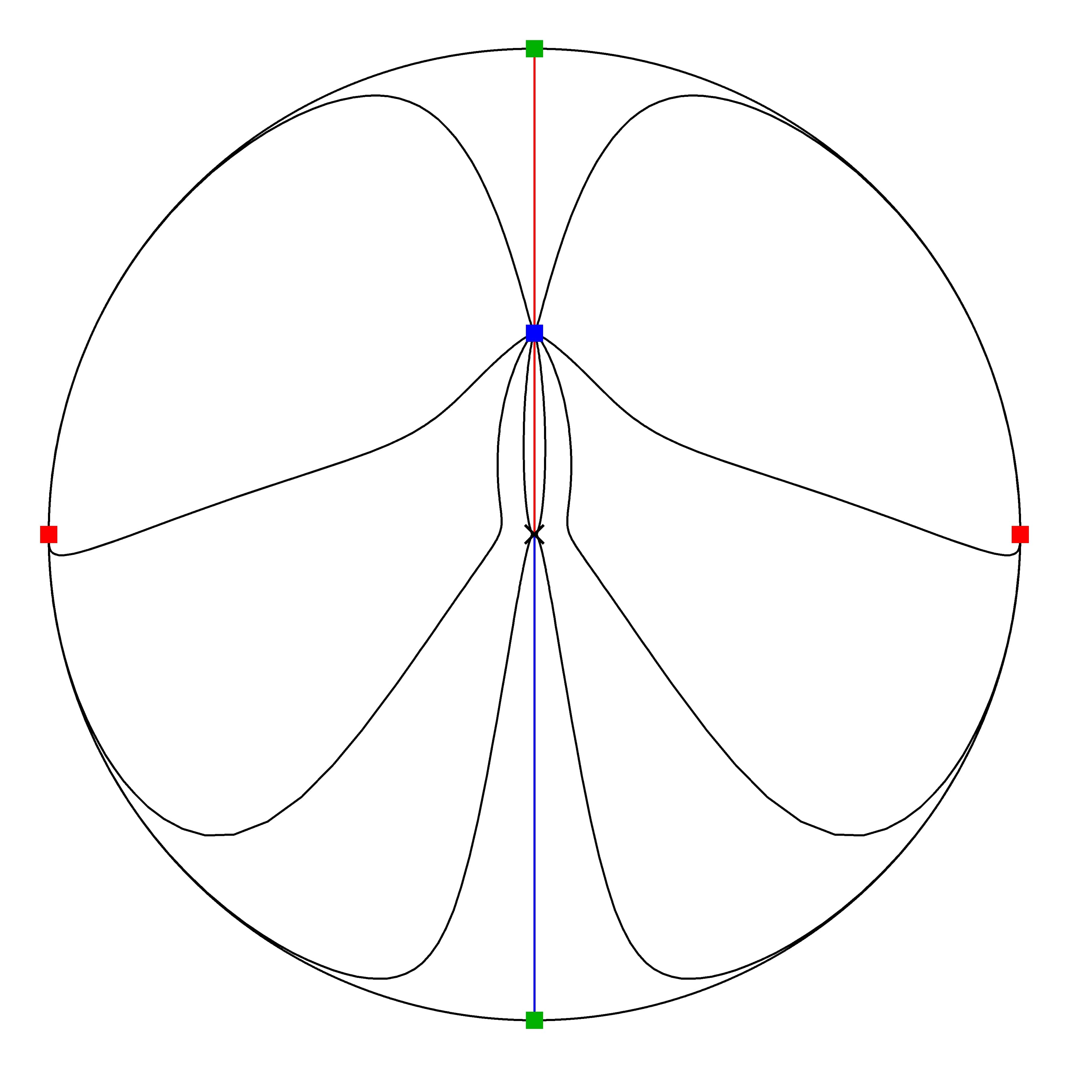
(f)  $a=2.5,\ b=1.9$

Figure 11: Phase portraits of the CDK system for $b=1.9$ and different values of $a$

   2. For $a<1<b$ and $|8a(a-1)|>b$ the stationary point $s_{1}$ has dynamics as in (2) of Lemma 4.3 and the stationary point $s_{2}$ is a saddle point. The stationary points $s_{3}$ and $s_{4}$ are strong attracting foci. The points at infinity in positive and negative $x$-direction are saddle points and the ones in positive and negative $y$-direction are repelling nodes (see Fig. 11(a)).

   3. For $a<1<b$ and $|8a(a-1)|\leq b$ the stationary point $s_{1}$ has dynamics as in (2) of Lemma 4.3 and the stationary point $s_{2}$ is a saddle point. The stationary points $s_{3}$ and $s_{4}$ are attracting nodes. The points at infinity in positive and negative $x$-direction are saddle points and the ones in positive and negative $y$-direction are repelling nodes (see Fig. 11(b)).

3. The dynamics of the system (7) for the parameter values as in (3) of Lemma 4.1 is:

   1. For $a=1$ and $1<b$ the stationary point $s_{1}$ has dynamics as in (2) of Lemma 4.3 and the stationary point $s_{2}$ is an attracting node. The points at infinity in positive and negative $x$-direction are saddle points and the ones in positive and negative $y$-direction are repelling nodes (see Fig. 11(c)).

   2. For $a=1$ and $b<1$ the stationary point $s_{1}$ has dynamics as in (1) of Lemma 4.3 and the stationary point $s_{2}$ is a saddle point where the $x$-direction is repelling and the $y$-direction attracting. The points at infinity in positive and negative $x$-direction are repelling nodes and the ones in positive and negative $y$-direction are saddle points (see Fig. 9(b)).

   3. For $1<a$, $1<b$ and $a=b$ the stationary point $s_{1}$ has dynamics as in (2) of Lemma 4.3 and the stationary point $s_{2}$ is an attracting node. At infinity every point is a stationary point (see Fig. 11(e)).

   4. For $1<a$, $1<b$ and $a<b$ the stationary point $s_{1}$ has dynamics as in (2) of Lemma 4.3 and the stationary point $s_{2}$ is an attracting node. The points at infinity in positive and negative $x$-direction are saddle points and the ones in positive and negative $y$-direction are repelling nodes (see Fig. 11(d)).

   5. For $1<a$, $1<b$ and $a>b$ the stationary point $s_{1}$ has dynamics as in (2) of Lemma 4.3 and the stationary point $s_{2}$ is an attracting node. The points at infinity in positive and negative $x$-direction are repelling nodes and the ones in positive and negative $y$-direction are saddle points (see Fig. 11(f)).

   6. For $a<1$, $b<1$ and $a=b$ the stationary point $s_{1}$ has dynamics as in (1) of Lemma 4.3 and the stationary point $s_{2}$ is a saddle where the $x$-direction is repelling and the $y$-direction is attracting. At infinity every point is a stationary point (see Fig. 9(d)).

   7. For $a<1$, $b<1$ and $a<b$ the stationary point $s_{1}$ has dynamics as in (1) of Lemma 4.3 and the stationary point $s_{2}$ is a saddle where the $x$-direction is repelling and the $y$-direction is attracting. The points at infinity in positive and negative $x$-direction are saddle points and the ones in positive and negative $y$-direction are repelling nodes (see Fig. 9(e)).

   8. For $a<1$, $b<1$ and $a>b$ the stationary point $s_{1}$ has dynamics as in (1) of Lemma 4.3 and the stationary point $s_{2}$ is a saddle where the $x$-direction is repelling and the $y$-direction is attracting. The points at infinity in positive and negative $x$-direction are repelling nodes and the ones in positive and negative $y$-direction are saddle points (see Fig.  9(c)).

   9. For $b=1$ and $a<1/2$ the stationary point $s_{1}$ has dynamics as in (3a) of Lemma 4.3 and the stationary point $s_{2}$ is a saddle where the $x$-direction is repelling and the $y$-direction is attracting. The points at infinity in positive and negative $x$-direction are saddle points and the ones in positive and negative $y$-direction are repelling nodes (see Fig. 10(b)).

   10. For $b=1$ and $a=1/2$ the stationary point $s_{1}$ has dynamics as in (3b) of Lemma 4.3 and the stationary point $s_{2}$ is is a saddle where the $x$-direction is repelling and the $y$-direction is attracting. The points at infinity in positive and negative $x$-direction are saddle points and the ones in positive and negative $y$-direction are repelling nodes (see Fig. 10(c)).

   11. For $b=1$ and $1/2<a<1$ the stationary point $s_{1}$ has dynamics as in (3c) of Lemma 4.3 and the stationary point $s_{2}$ is is a saddle where the $x$-direction is repelling and the $y$-direction is attracting. The points at infinity in positive and negative $x$-direction are saddle points and the ones in positive and negative $y$-direction are repelling nodes (see Fig. 10(d)).

   12. For $b=1$ and $1<a$ the stationary point $s_{1}$ has dynamics as in (3d) of Lemma 4.3 and the stationary point $s_{2}$ and the stationary point $s_{2}$ is an attracting node. The points at infinity in positive and negative $x$-direction are repelling nodes and the ones in positive and negative $y$-direction are saddle points (see Fig. 10(e)).

5 Phase Portraits and Bifurcations of the CDK System

The above analysis of the stationary points distinguishes 16 different regions in the positive quadrant of the parameter plane. These are shown in Fig. 7 with $a$ on the horizontal axis and $b$ on the vertical one. The description in the various regions corresponds to the numbering of the different cases in Theorem 4.6. One immediately sees that the main case distinctions arise whenever one of the parameter crosses the value $1$.

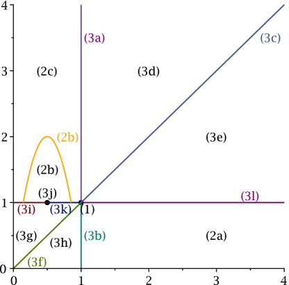
Figure 7: The different cases in the positive orthant of the parameter plane

Figs. 9-11 in the appendix contain for each arising case a typical phase portrait. These phase portraits have been generated with the help of P4 (see [Dumortier et al., 2006, Chapt. 9] for more information on this programme). The phase portraits are shown on the Poincaré disc, i. e. the infinite plane $\mathbbm{R}^{2}$ is mapped into a finite disc (see [Dumortier et al., 2006, Chapt. 5] for more details about the used transformation), as this allows to depict also the stationary points at infinity. In the plots, curves in green or cyan consist entirely of stationary points; curves in red or blue are separatrices. A green square signals a saddle, a blue square a stable node and a red square an unstable node. Finally, a blue diamond marks a stable strong focus, a blue triangle a semi-hyperbolic stable node, a green triangle a semi-hyperbolic saddle and a black x a non-elementary stationary point.

The changes of the phase portraits concern several aspects. We will mainly consider the number of stationary points and their types, the number of attractors and the existence of homoclinic orbits. The latter point is controlled exclusively by the parameter $b$. Therefore we organise our discussion by the value of $b$. We will not consider all 16 cases separately, as sometimes the differences are fairly minor. In particular, in most cases the relative size of $a$ and $b$ only affects the stationary points at infinity. For $a=b$, all points at infinity are stationary. Otherwise, there are two stationary points at infinity (antipodes on the boundary of the Poincaré disc can be identified): a saddle and an unstable node which switch their positions depending on whether $a<b$ or $b<a$. We always find either one or two “almost attractors”. These are stationary points and almost all trajectories end in them, the sole exceptions being trajectories lying in the stable manifolds of saddle points.

We begin with the case $b<1$ shown in Fig. 9. A key feature of the phase portraits is the existence of the two elliptic sectors at the origin with infinitely many homoclinic orbits. One effect of them is that the index of the vector field (6) at the origin $s_{1}$ is $2$. For $a>1$, $s_{2}$ is a stable node and there are the two additional finite stationary points $s_{3/4}$ which are saddle points (see Fig. 9(a)). We have here two “almost attractors”, namely $s_{1}$ and $s_{2}$. The stable manifolds of the saddle points $s_{3/4}$ separate their basins of attraction. Furthermore, in this case, infinitely many heteroclinic orbits connect $s_{1}$ with $s_{2}$. When $a$ approaches $1$, then $s_{3/4}$ move towards $s_{2}$. When $b$ approaches $1$, then they move towards $s_{1}$. If $a$ and $b$ simultaneously approach $1$, then $s_{3}$ and $s_{4}$ move both towards some points on the circle of stationary points arising for $a=b=1$ (see below) depending on the precise relationship between $a$ and $b$ in the limit process. For $a=1$, $s_{3/4}$ have coalesced with $s_{2}$ to a semihyperbolic saddle and the heteroclinic orbits connecting $s_{1}$ with $s_{2}$ have all disappeared except for the one representing a part of the stable manifold of the saddle. The separatrix forming the boundary of the elliptic sectors is now a centre manifold of the semihyperbolic saddle (not shown in Fig. 9(b)). For $a\leq 1$, the origin $s_{1}$ is the sole “almost attractor” of the system (Figs. 9(b)-9(e)).

Now we consider the “border case” $b=1$ shown in Fig. 10. Here we find a very special situation, if also $a=1$ (see Fig. 10(a)). Then the two components of the vector field (6) have a common factor leading to infinitely many finite stationary points, namely all points on the circle $x^{2}+(y-1/2)^{2}=1/4$ (note that $s_{1}$ and $s_{2}$ both lie on this circle). As always for $a=b$, we also find infinitely many stationary points at infinity. All trajectories starting at a point $(x_{0},y_{0})$ with $y_{0}\leq 0$ or at a point inside this circle end in $s_{1}$. All other trajectories connect a stationary point at infinity with a stationary point on the circle. If $a<1$, then we find again the two elliptic sectors at the origin and thus again the index of the vector field (6) at $s_{1}$ is $2$. The three cases shown in Fig. 10(b)-10(d) differ only in the computational analysis of the non-elementary stationary point $s_{1}$ which in two cases yields two additional separatrices. However, each of these separatrices only separates two parabolic sectors and thus they have no real influence on the qualitative form of the phase portrait. We always have $s_{1}$ as sole “almost attractor” of the system. For $a>1$ (see Fig. 10(e)), $s_{2}$ becomes a stable node attracting all trajectories starting in the upper half plane. All other trajectories continue to end in $s_{1}$. The elliptic sectors become parabolic and contain infinitely many heteroclinic orbits connecting $s_{1}$ with $s_{2}$.

Finally, we consider the case $b>1$ shown in Fig. 11. Here no elliptic sectors exists and thus no homoclinic orbits. Furthermore, now the index of the vector field (6) at the origin is $0$. If $a<1$, then there are two additional stationary points $s_{3}$ and $s_{4}$ (see Figs. 11(a) and 11(b)). Depending on the relative size of $a$ and $b$, they are either stable focii or stable nodes. In particular, they are the only attractors of the system. For $a$ oder $b$ (or both) approaching $1$, we find the same behaviour as in the case $b<1$ (except that the approach is now for both parameters from the other side of $1$). For $a=1$, $s_{3/4}$ have coalesced with $s_{2}$ to a semihyperbolic stable node (Fig. 11(c)) and whenever $a\geq 1$, then $s_{2}$ is the sole attractor of the system (Figs. 11(c)-11(e)).

It follows from our discussion of the stationary points at infinity in Section 4.5 that all forward orbits remain bounded, as no point at infinity has incoming trajectories. This fact was already mentioned by Alvarez-Ramirez et al. [2005], however, with an erroneous argument. They claim – using a Lyapunov type argument – that any forward orbit converges into a circle with the radius $r=\sqrt{\max{\{a^{-2},\tfrac{2-b}{b^{2}}\}}}$. However, this is not true, as for large values of $a$ and $b$, this radius can be made arbitrarily small, nevertheless Lemma 4.2 shows that for these parameter values the point $(0,1)$ is an attracting node. If one chooses e.g. $a=2.5$, $b=1.9$ (cf. Fig. 11(f)) and considers the point $(0.1,0.9)$ which lies outside a circle of radius $r=0.4$, then one easily checks that the derivative $\dot{V}$ of their Lyapunov function is positive at this point despite the opposite claim of Alvarez-Ramirez et al. [2005].

For large values of $b$ and small values of $a$, the radius $r$ determined by Alvarez-Ramirez et al. [2005] becomes arbitrarily large. This is indeed necessary, as for $b>1>a$ one is in case (2) of Lemma 4.1 where the additional stationary points $s_{3/4}$ exist and these are both attractive by Lemma 4.4. It is easy to see that for a fixed value of $b>1$ and for $a\rightarrow 0$ the absolute value of the $x$-coordinates of these points given by (13) becomes arbitrarily large.

6 General Rational Systems

So far, we concentrated in this article on the CDK system. Now we want to discuss briefly the case of a general planar system with a rational right hand side. Let the system be of the form

$$\dot{x}=\frac{p}{q}\,,\qquad\dot{y}=\frac{r}{s}$$ (16)

where $p$, $q$, $r$, $s$ are polynomials in $x$ and $y$ and where we assume for simplicity that in both equations numerator and denominator are relatively prime. Again it is for our purposes more convenient to rewrite the system in the implicit form

$$q\dot{x}=p\,,\qquad s\dot{y}=r\,.$$ (17)

In the CDK system we are in the special situation that $q=s$ which provides a minor simplification compared to the general case.

If we introduce $\ell=\operatorname{lcm}{(q,s)}$, a least common multiple of the two denominators, and write $\ell=q\bar{q}=s\bar{s}$, then a straightforward computation analogous to the one detailed above yields as generator for the projected Vessiot distribution the vector field

$$Y=\ell\partial_{t}+\bar{q}p\partial_{x}+\bar{s}r\partial_{y}\,.$$ (18)

This is actually a minimal generator. Indeed, by definition of a least common multiple $\gcd{(\bar{q},\bar{s})}=1$. Furthermore, $\gcd{(\ell,\bar{q}p)}=\bar{q}$ and $\gcd{(\ell,\bar{s}r)}=\bar{s}$, since we assumed that our right hand sides are in reduced form. Hence $\gcd{(\ell,\bar{q}p,\bar{s}r)}=1$.

Again one can decouple the $t$-component and thus finds that the trajectories of (16) are the same as the ones of the polynomial system

$$\dot{x}=\bar{q}p\,,\qquad\dot{y}=\bar{s}r\,.$$ (19)

However, because of the decoupling, we can no longer assume that the right hand sides are relatively prime. If $d=\gcd{(p,r)}$ is a non-constant polynomial, then all zeros of $d$ are stationary points leading to a situation similar to the case $a=b=1$ in the CDK system. The system (19) can now be completely analysed in the same manner, as we did for the CDK system.

7 A Logarithmic Variant of the CDK System

Sprott [2010, Sect. 5.3] presented further “chaotic” two-dimensional systems. Some are just minor variations of the CDK system. We have not analysed them all, but the phase portraits shown in [Sprott, 2010, Sect. 5.3] clearly indicate that most probably all of these systems also exhibit elliptic sectors instead of chaos. Finally, Sprott produced a logarithmic “chaotic” system:

$$\dot{x}=\frac{1}{2}\ln{(x^{2})}-y\,,\qquad\dot{y}=\frac{1}{2}\ln{(x^{2})}+x\,.$$ (20)

It is defined only away from the $y$-axis, as for $x=0$ the logarithmic term becomes infinite. Again it is trivial to show that this system cannot exhibit any chaotic behaviour. Multiplication of the right hand side of (20) by $x^{2}$ yields a system which has the same orbits away from the $y$-axis and which is everywhere in the plane defined and $C^{1}$. Thus the Poincaré-Bendixson Theorem applies and excludes chaotic behaviour. For a more detailed analysis of the behaviour near the $y$-axis, we cannot use the same approach as in the main text. However, it turns out that very elementary considerations suffice.

Figure 8 shows some streamlines and the nullclines of system (20). One clearly sees the one stationary point of the system at $\bigl{(}W(1),-W(1)\bigr{)}\cong(0.56714,-0.56714)$ where $W$ denotes the Lambert $W$ function. It is an unstable focus. The $y$-nullcline is the straight line $x=W(1)$, whereas the $x$-nullcline consists of the two branches of $y=\ln{|x|}$. The streamlines cross the $y$-axis smoothly with the constant slope $1$, since

$$\lim_{(x,y)\rightarrow(0,y_{0})}{\frac{dy}{dx}}=\lim_{(x,y)\rightarrow(0,y_{0})}{\frac{1+2x/\ln{x^{2}}}{1-2y/\ln{x^{2}}}}=1$$ (21)

for any value of $y_{0}$. As the two branches of the $x$-nullcline are converging towards the negative $y$-axis for $x\rightarrow 0$, in the neighbourhood of a point $(0,y_{0})$ with $y_{0}$ a large negative number the streamlines are rapidly changing from almost vertical to slope $1$ to again almost vertical. The “chaos” observed by Sprott is therefore nothing but a consequence of problems in numerically resolving the dynamics in such a region with a rapidly changing vector fields.

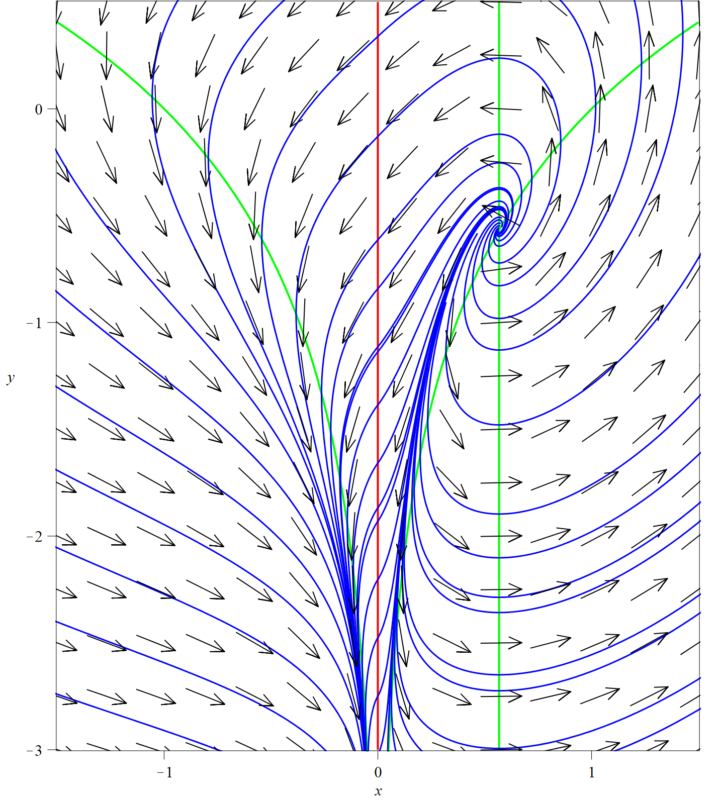
Figure 8: Streamlines and nullclines for system (20)

8 Conclusions

In our opinion, the use of the term “chaos” in the context of the CDK system is based on some misconceptions about its mathematical meaning. Firstly, not every (highly) irregular dynamics is chaotic. Secondly, chaotic behaviour is a property of the exact trajectories of a dynamical system and not concerned with numerical difficulties in their determination or with the effect of noise. Precise definitions differ from author to author. A classical and very popular one goes back to Devaney [1989, Def. 8.5]. In the version given by Wiggins [2003, Def. 30.0.2], one expects the following three properties from a (compact) chaotic invariant set $\Lambda$ (see also the discussion in [Katok & Hasselblatt, 1995, Def. 7.2.1]): (i) the flow exhibits a sensitive dependence on initial conditions everywhere on $\Lambda$, (ii) $\Lambda$ is topologically transitive and (iii) periodic orbits are dense in $\Lambda$. Wiggins [2003] also provides a series of examples demonstrating the importance of each aspect of these conditions. In the case of the CDK system, none of these three properties is actually given – even if one restricts to the union of the two elliptic sectors as a compact invariant set.

In the CDK system for $b<1$ and in Sprott’s logarithmic variant one finds the following situation. The systems exhibit a sensitive dependence on initial conditions only in very small regions: for the CDK system, these regions include in particular that part of the elliptic sectors which is very close to the origin; in the logarithmic variant, it is a tubular neighbourhood of the $y$-axis for sufficiently large negative values. This fact alone would not lead to the observed very irregular trajectories. The second key ingredient is that trajectories leaving the respective sensitive region will reenter it after a finite time. In the CDK system, this fact is due to the ellipticity of the sectors and thus the existence of homoclinic orbits. In the logarithmic variant, the unstable focus is mainly responsible for this behaviour.

If one tries in such a situation to integrate numerically one of the trajectories starting in the respective sensitive region “until the end”, then it is almost unavoidable that at some stage numerical errors lead to a jump from any incoming trajectory to an outgoing one. As after a finite time, this outgoing trajectory will become again an incoming one, the same will happen repeatedly. This simple observation explains the highly irregular behaviour seen in some numerical simulations without any resort to chaotic dynamics. One should, however, always keep in mind that the thus obtained numerical curves do not approximate a single trajectory, but a “concatenation” of many different ones (and thus such curves cannot be used to estimate Lyapunov exponents of single trajectories).

This phenomenon will appear in any two-dimensional system with a stationary point possessing at least one elliptic sector (which is possible only at non-elementary stationary points). If noise is added to such a system, it can indeed model highly irregular dynamics without being chaotic and constructing such a model was the original goal of Cummings et al. [1992]. The term “piecewise deterministic dynamics” coined later by Dixon [1995] is for such behaviour much more appropriate than “chaos”.

The existence of elliptic sectors for the CDK system was already observed by Alvarez-Ramirez et al. [2005]. In contrast to claims by Sprott [2010] and Alvarez-Ramirez et al. [2005], the union of the two elliptic sectors does not define a two-dimensional attractor, but solely an attracting set. One of the simplest definition of an attractor (see e. g. [Perko, 2001, Def. 1, Sect. 3.2]) says that it is an attracting set which contains a dense orbit. Obviously, this is not the case here. In the relevant region in the parameter space, the CDK system does not possess at all an attractor (the origin attracts almost all trajectories in its neighbourhood – except the ones starting on the positive $y$-axis), an observation which again excludes the existence of chaos.

The main contribution of this article is a complete bifurcation analysis of the CDK system. While Cummings et al. [1992] distinguished for their numerical experiments only four regions in the parameter space, we showed that including the behaviour at infinity leads actually to sixteen different regions in the parameter space. If one studies only a finite neighbourhood of the origin, then essentially one finds only the four cases of Cummings et al. [1992] (plus the boundary cases). The only exception is a subtle difference in the phase portraits for $b>1$ and $a<1$ where depending on the value of $a$ the additional stationary points $s_{3}$ and $s_{4}$ exhibit slightly different behaviour. Given the great symmetry of the CDK system and the fact that physically the parameters $a$, $b$ represent very similar quantities, it is remarkable that the two parameters possess completely different roles in the bifurcation analysis. The appearance of the elliptic sectors is controlled exclusively by $b$, whereas $a$ determines the behaviour at infinity.

Acknowledgments The authors thank Peter de Maesschalck (Hasselt University) and Sebastian Walcher (RWTH Aachen) for many helpful discussions about dynamical systems and Oscar Saleta Reig (Universitat Autònoma de Barcelona) for helping with P4. This work was supported by the bilateral project ANR-17-CE40-0036 and DFG-391322026 SYMBIONT.

Appendix: Phase Portraits for the Various Cases

For each case arising in Theorem 4.6, we have produced a numerical phase portrait using P4 for one specific set of parameter values in the corresponding region of the parameter space. A discussion of the phase portraits and an explanation of the used symbols has already been given in Section 5.

References

- Alvarez-Ramirez et al. [2005] Alvarez-Ramirez, J., Delgado-Fernandez, J. & Espinosa-Paredes, G. [2005] “The origin of a continuous two-dimensional ”chaotic” dynamics,” Int. J. Bif. Chaos 15, 3023–3029.
- Arnold [1988] Arnold, V. [1988] Geometrical Methods in the Theory of Ordinary Differential Equations, ed., Grundlehren der mathematischen Wissenschaften 250 (Springer-Verlag, New York).
- Cummings et al. [1992] Cummings, F., Dixon, D. & Kaus, P. [1992] “Dynamical model of the magnetic field of neutron stars,” Astrophys. J. 386, 215–221.
- Devaney [1989] Devaney, R. [1989] An Introduction to Chaotic Dynamical Systems, ed. (Addison-Wesley, Redwood City).
- Dixon [1995] Dixon, D. [1995] “Piecewise deterministic dynamics from the application of noise to singular equations of motion,” J. Phys. A: Math. Gen. 28, 5539–5551.
- Dixon et al. [1993] Dixon, D., Cummings, F. & Kaus, P. [1993] “Continuous “chaotic” dynamics in two dimensions,” Physica D 65, 109–116.
- Dumortier et al. [2006] Dumortier, F., Llibre, J. & Artés, J. [2006] Qualitative Theory of Planar Differential Systems, Universitext (Springer-Verlag, Berlin).
- Fackerell [1985] Fackerell, E. [1985] “Isovectors and prolongation structures by Vessiot’s vector field formulation of partial differential equations,” Geometric Aspects of the Einstein Equations and Integrable Systems, ed. Martini, R., Lecture Notes in Physics 239 (Springer-Verlag, Berlin), pp. 303–321.
- Guckenheimer & Holmes [1990] Guckenheimer, J. & Holmes, P. [1990] Nonlinear Oscillations, Dynamical Systems, and Bifurcations of Vector Fields, Applied Mathematical Sciences 42 (Springer-Verlag, New York).
- Katok & Hasselblatt [1995] Katok, A. & Hasselblatt, B. [1995] Introduction to the Modern Theory of Dynamical Systems, Encyclopedia of Mathematics and its Applications 54 (Cambridge University Press, Cambridge).
- Perko [2001] Perko, L. [2001] Differential Equations and Dynamical Systems, 3rd ed., Texts in Applied Mathematics 7 (Springer-Verlag).
- Seiler [2010] Seiler, W. [2010] Involution — The Formal Theory of Differential Equations and its Applications in Computer Algebra, Algorithms and Computation in Mathematics 24 (Springer-Verlag, Berlin).
- Seiler [2013] Seiler, W. [2013] “Singularities of implicit differential equations and static bifurcations,” Computer Algebra in Scientific Computing — CASC 2013, eds. Gerdt, V., Koepf, W., Mayr, E. & Vorozhtsov, E., Lecture Notes in Computer Science 8136 (Springer-Verlag, Berlin), pp. 355–368.
- Seiler & Seiß [2018] Seiler, W. & Seiß, M. [2018] “Singular initial value problems for scalar quasi-linear ordinary differential equations,” Preprint Kassel University.
- Sijbrand [1985] Sijbrand, J. [1985] “Properties of center manifolds,” Trans. AMS 289, 431–469.
- Sprott [2010] Sprott, J. [2010] Elegant Chaos (World Scientific, Hackensack).
- Vessiot [1924] Vessiot, E. [1924] “Sur une théorie nouvelle des problèmes généraux d’intégration,” Bull. Soc. Math. Fr. 52, 336–395.
- Wiggins [2003] Wiggins, S. [2003] Introduction to Applied Nonlinear Dynamical Systems and Chaos, ed., Text in Applied Mathematics 2 (Springer-Verlag, New York).