Objective barriers to the transport of dynamically active vector fields

Abstract

We derive a theory for material surfaces that maximally inhibit the diffusive transport of a dynamically active vector field, such as the linear momentum, the angular momentum or the vorticity, in general fluid flows. These special material surfaces (Lagrangian active barriers) provide physics-based, observer-independent boundaries of dynamically active coherent structures. We find that Lagrangian active barriers evolve from invariant surfaces of an associated steady and incompressible barrier equation, whose right-hand side is the time-averaged pullback of the viscous stress terms in the evolution equation for the dynamically active vector field. Instantaneous limits of these barriers mark objective Eulerian active barriers to the short-term diffusive transport of the dynamically active vector field. We obtain that in unsteady Beltrami flows, Lagrangian and Eulerian active barriers coincide exactly with purely advective transport barriers bounding observed coherent structures. In more general flows, active barriers can be identified by applying Lagrangian coherent structure (LCS) diagnostics, such as the finite-time Lyapunov exponent and the polar rotation angle, to the appropriate active barrier equation. In comparison to their passive counterparts, these active LCS diagnostics require no significant fluid particle separation and hence provide substantially higher-resolved Lagrangian and Eulerian coherent structure boundaries from temporally shorter velocity data sets. We illustrate these results and their physical interpretation on two-dimensional, homogeneous, isotropic turbulence and on a three-dimensional turbulent channel flow.

1 Introduction

Fluid transport is often the simplest to describe through its barriers. Indeed, transport barriers are routinely invoked in discussions of transport in classical fluid dynamics (Ottino 1989), geophysics (Weiss & Provenzale 1989), reactive flows (Rosner 2000) and plasma fusion (Dinklage 2005).

Despite their broadly recognized significance, transport barriers have remained loosely defined and little understood. The only generally agreed definition is the one of MacKay, Meiss & Percival (1984) who define transport barriers in two-dimensional (2D), time-periodic flows as invariant curves of the Poincaré (or stroboscopic) map for fluid particle motions. This definition extends to three-dimensional (3D) steady flows, identifying advective transport barriers as 2D material surfaces whose intersection with a section transverse to the flow is an invariant curve for the first-return map defined for that section (Ottino 1989, MacKay 1994). In many 3D steady flows, however, trajectories may rarely if ever return to the physically relevant Poincaré sections, such as the cross-stream sections of pipe flows.

This lack of returns obliges one to look for barriers to advective transport among all material surfaces – an ill-defined objective, given that all material surfaces are barriers to advective transport. Indeed, none of them can be crossed by other material trajectories by the uniqueness of trajectories through any point at a given time in a smooth velocity field. Some material surfaces are nevertheless perceived as organizers of advective transport because they preserve their coherence, i.e., do not develop smaller scales (filamentation) in their evolution. These distinguished surfaces are generally referred to as Lagrangian coherent structures (or LCS; see Haller 2015). In the absence of a universally accepted notion of material coherence, however, different LCS definitions continue to coexist and highlight different material surfaces as advective transport barriers (Hadjighasem et al. 2017). Beyond their diversity, most LCS criteria have also been criticized for being purely kinematic with no regard to relevant physical quantities, such as the linear momentum and the vorticity. The need for developing LCS methods for the transport of such physical quantities has recently been stressed by Balasuriya, Ouellette & Rypina (2018).

Parallel to the development of different LCS criteria, several different Eulerian criteria for coherent vortices have been put forward (see Epps 2017 and Günther & Theisel 2018 for recent reviews). Most of these approaches also set out to find sustained (Lagrangian) swirling motion of fluid particles, but hope to achieve this goal by studying local properties of instantaneous (Eulerian) velocity snapshots. As this is a hopeless undertaking for unsteady flows, these approaches invariably divert from their originally stated objective and postulate coherence principles for the instantaneous velocity field, rather than for particle motion. One can then a posteriori interpret the resulting velocity-dependent inequalities (such as the $Q$-, $\Delta$-, $\lambda_{2}$ - and $\lambda_{ci}$-criteria reviewed recently in Pedergnana et al. 2020) as physical, but their actual connection to flow physics is unclear due to the conceptual gaps in their derivations and their dependence on the observer,

Unsurprisingly, therefore, the resulting vortex criteria often yield erroneous results even for simple flows in which the coherent swirling regions can be identified unambiguously from Poincaré maps (see Pedergnana et al. 2020 for recent demonstrations). This has resulted in the practice of plotting a few level sets of $Q$, $\Delta$, $\lambda_{2}$ or $\lambda_{ci}$, as opposed to verifying the inequalities imposed on these quantities by the appropriate criteria (see, e.g., Dubief & Delcayre 2000, McMullan & Page 2012, Anghan et al. 2014, Gao et al. 2015, Jantzen et al. 2019). These level surfaces are selectively chosen to match expectations or produce visually pleasing images. As a further ad hoc element in this procedure, the level surfaces are not objective: they depend on the frame of reference, even though truly unsteady flows have no distinguished frame of reference (Lugt 1979). The experimental detectability or physical relevance of these surfaces is, therefore, unclear. Arguably, as long as this practice continues, there is little hope for a commonly accepted definition for coherent vortices.

A way out of this conundrum is to identify coherent structures based on the transport of physical quantities of interest to the fluid mechanics community, but use mathematical deductions that are free from ad hoc assumptions, user-defined thresholds and tunable parameters. Specifically, one may seek the boundaries of coherent structures or vortices based on their transport-extremizing properties. Unlike the notions of coherence and swirling, the notion of transport through a surface is physically well-understood, quantitative and frame-independent, when properly phrased. These features allow for a systematic, quantitative comparison of all surfaces to find minimizers (barriers) of transport among them. This in turn offers a way to quantify the general view in fluid mechanics that coherent structures influence transport processes in turbulent flows (Robinson 1991, Hutchins & Marusic 2007).

As a first step in this direction, Haller, Karrasch & Kogelbauer (2018, 2019) formalize the definition of transport barriers for passively advected diffusive scalars. They then locate transport barriers as material surfaces that inhibit the diffusive transport of a weakly diffusive scalar more than neighboring material surfaces do. Katsanoulis et al. (2019) use these results to locate vortex boundaries in 2D flows as outermost closed barriers to the diffusive transport of the scalar vorticity. These results, however, do not cover barriers to the transport of dynamically active vector fields, such as momentum and vorticity, in 3D. There are also examples, such as the 2D decaying channel flow shown in Fig. 1, in which the passive-scalar-based approach to vorticity transport only captures the walls as perfect transport barriers in a finite-time analysis. The remaining observed barriers to the redistribution of the normalized vorticity (i.e., all horizontal lines) are only captured by the approach over an infinitely long time interval.

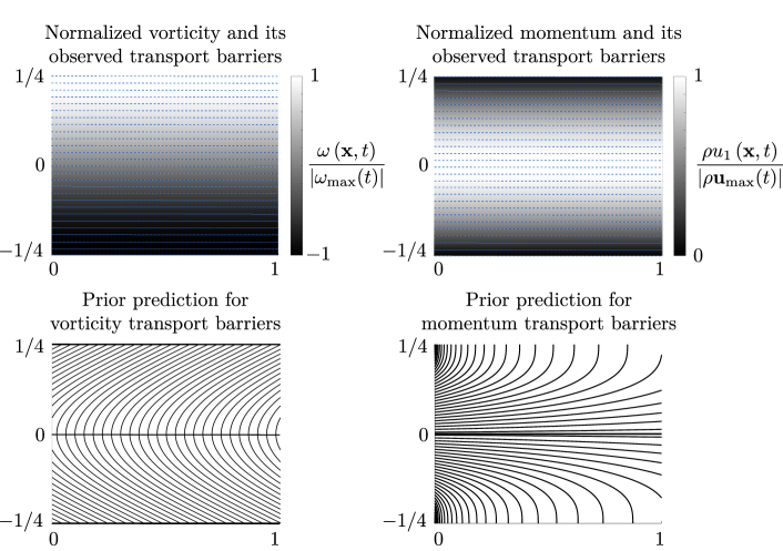
Figure 1: Vorticity and linear momentum, normalized by their maxima at an arbitrary time instance in a decaying planar channel flow. These plots remain steady in time, with all horizontal lines (some shown dotted) acting as barriers to the vertical redistribution of the vorticity and linear momentum. Also shown are prior predictions for perfect barriers to vorticity transport in this flow by Haller, Karrasch & Kogelbauer (2019) on the left and for perfect barriers to momentum transport by Meyers & Meneveau (2013) on the right. The latter barrier trajectories are released uniformly across the entry cross section of the channel. See Appendix A for details.

More broadly speaking, there has been a lack of methods to identify barriers to the transport of dynamically active quantities, i.e., scalar, vector or tensor fields whose evolution impacts the evolution of the underlying fluid velocity field. A notable exception is the work of Meyers & Meneveau (2013), who locate momentum- and energy-transport barriers as tubes tangent to a flux vector field formally associated with these dynamically active scalar fields. While insightful, this approach also has several heuristic elements. The construct depends on the frame of reference and the choice of a transport direction. The flow data is assumed statistically stationary with a well-defined mean velocity field. The proposed flux vector introduced in this fashion is non-unique: any divergence-free vector field could be added to it. Finally, the flux vector differs from the classic momentum and energy flux that it purports to represent. All these features of the approach prevent the detection of most observed barriers to momentum redistribution already in simple 2D flows, such as our 2D decaying channel flow example in Fig. 1. Indeed, the only horizontal barrier captured by this approach is the symmetry axis of the channel.

In the present work, we seek to fill the gaps in previous approaches by extending the transport-barrier-detection approach of Haller, Karrasch & Kogelbauer (2018, 2019) to active transport in 3D. In this extension, we seek material barriers to the diffusive (or viscosity-induced) transport of an arbitrary dynamically active vector field, by which we mean a vector field whose evolution impacts the evolution of the underlying fluid velocity field. We then seek transport barriers as special material surfaces across which the net diffusive transport of the active vector field pointwise vanishes. When applied to the 2D channel flow example shown in Fig. 1, the approach we develop here returns the observed material barriers (all horizontal lines) as barriers to the spatial redistribution of vorticity and momentum (see Example 7.3 in section 7.1). This example and more complex examples discussed later illustrate that material barriers to active transport can be used to define boundaries of dynamical coherent structures (i.e., time-varying structures observed in dynamically active vector fields) in a frame-independent fashion.

The outline of this paper is as follows. In section 2, we introduce our set-up and notation for a dynamically active vector field. We then discuss in section 3 the shortcomings of available flux definitions when applied to active transport through material surfaces, and introduce an objective notion of diffusive transport for active vector fields. In section 4, we identify surfaces blocking this diffusive transport and define active transport barriers more formally. Section 5 describes the instantaneous, Eulerian limits of these active barriers, and section 6 derives the equations for both Lagrangian and Eulerian active barriers to the diffusive transport of linear momentum, angular momentum and vorticity. In section 7, we work out solutions of these barrier equations analytically for 2D Navier–Stokes flows and 3D directionally steady Beltrami flows. Section 8 discusses computational aspects of active transport barriers and introduces active versions of passive LCS-detection tools that generally enable a higher-resolved identification of coherent structures from finite-time flow data than their passive counterparts do. Section 9 shows such computations and their physical implications for 2D homogeneous, isotropic turbulence and for a 3D turbulent channel flow. We summarize our conclusions in section 10. Appendix A illustrates on a simple example the challenges of defining active barriers with an observable footprint. Appendix B motivates the need for a new definition for diffusive flux through material surfaces. Finally, Appendices C and D contain the detailed proofs of our technical results.

2 Set-up

We consider a 3D flow with velocity field $\mathbf{u}(\mathbf{x},t)$ and density $\rho(\mathbf{x},t)$, known at spatial locations $\mathbf{x}\in U\in\mathbb{R}^{3}$ in a bounded set $U$ at times $t\in\left[t_{1},t_{2}\right]$. The equation of motion for such a flow is of the general form

$$\rho\frac{D\mathbf{u}}{Dt}=-\bm{\nabla}p+\bm{\nabla}\cdot\mathbf{T}_{vis}+\mathbf{q},$$ (1)

where $D/Dt$ denotes the material derivative, $p(\mathbf{x},t)$ is the (equilibrium) pressure, $\mathbf{T}_{vis}(\mathbf{x},t)=\mathbf{T}_{vis}^{T}(\mathbf{x},t)$ is the viscous stress tensor and $\mathbf{q}(\mathbf{x},t)$ denotes the external body forces (see Gurtin, Fried & Anand 2013).

Material trajectories generated by the velocity field $\mathbf{u}$ are solutions of the differential equation $\dot{\mathbf{x}}=\mathbf{u}(\mathbf{x},t)$. We denote the time-$t$ position of a trajectory starting from $\mathbf{x}_{0}$ at time $t_{0}$ by $\mathbf{x}(t;t_{0},\mathbf{x}_{0})$. The flow map induced by $\mathbf{u}$ is defined as the mapping $\mathbf{F}_{t_{0}}^{t}\colon\mathbf{x}_{0}\mapsto\mathbf{x}(t;t_{0},\mathbf{x}_{0})$. A material surface $\mathcal{M}(t)\subset U$ is a time-dependent two-dimensional manifold transported by the flow map from its initial position $\mathcal{M}_{0}:=\mathcal{M}(t_{0})$ as

$$\mathcal{M}(t)=\mathbf{F}_{t_{0}}^{t}\left[\mathcal{M}(t_{0})\right].$$ (2)

Let $\mathbf{f}(\mathbf{x},t)$ be another smooth vector field defined on the same spatiotemporal domain $U\times\left[t_{0},t_{1}\right]$. We will be interested in $\mathbf{f}$ fields that are dynamically active vector fields, i.e., their evolution impacts the evolution of the velocity field $\mathbf{u}$. Such a vector field $\mathbf{f}$ is typically defined as a function of $\mathbf{u}$ and its derivatives. The simplest physical examples of active vector fields are the linear momentum $\mathbf{f}:=\rho\mathbf{u}$ and the vorticity $\mathbf{f}:=\bm{\omega}=\bm{\nabla}\times\mathbf{u}$. Both of these examples of $\mathbf{f}$ are frame-dependent (non-objective) vector fields, because they do not transform properly under general frame changes of the form

$$\mathbf{x}=\mathbf{Q}(t)\mathbf{y}+\mathbf{b}(t),\quad\mathbf{QQ}^{T}=\mathbf{I},\quad\mathbf{Q}(t)\in SO(3),\quad\mathbf{b}(t)\in\mathbb{R}^{3},$$ (3)

where both $\mathbf{Q}(t)$ and $\mathbf{b}(t)$ are smooth in time. Indeed, evaluating the definition of these vectors in the $\mathbf{y}$-frame gives transformed vector fields $\tilde{\mathbf{f}}(\mathbf{y},t)$ for which

$$\tilde{\mathbf{f}}(\mathbf{y},t)\neq\mathbf{Q}^{T}(t)\mathbf{f}(\mathbf{x},t).$$ (4)

It is, therefore, a challenge to describe the transport of $\mathbf{f}$ through a material surface in an intrinsic, observer-independent fashion.

We assume that the evolution of $\mathbf{f}$ is governed by a partial differential equation of the form

$$\frac{D}{Dt}\mathbf{f}=\mathbf{h}_{vis}+\mathbf{h}_{nonvis},\qquad\partial_{\mathbf{T}_{vis}}\mathbf{h}_{vis}\neq\mathbf{0},\quad\partial_{\mathbf{T}_{vis}}\mathbf{h}_{nonvis}=\mathbf{0}.$$ (5)

The function $\mathbf{h}_{vis}(\mathbf{x},t,\mathbf{u},\mathbf{f},\mathbf{T}_{vis})$ contains all the terms arising from diffusive forces (i.e., viscous Cauchy stresses), while $\mathbf{h}_{nonvis}(\mathbf{x},t,\mathbf{u},\mathbf{f})$ has no explicit dependence on those forces. Instead, $\mathbf{h}_{nonvis}$ contains terms originating from the pressure, external forces and possible inertial effects. For instance, as we will see in section 6, when $\mathbf{f}$ is the linear momentum of an incompressible Navier–Stokes flow with kinematic viscosity $\nu$, then we have $\mathbf{h}_{vis}:=\rho\nu\Delta\mathbf{u}$. Or if, for the same class of flows, $\mathbf{f}$ equals the vorticity $\bm{\omega}=\bm{\nabla}\times\mathbf{u}$ , then we have $\mathbf{h}_{vis}:=\nu\Delta\bm{\omega}$.

We finally assume that $\mathbf{h}_{vis}$ is an objective vector field, i.e., under any observer change of the form (3), we obtain the transformed vector field $\mathbf{\tilde{h}}_{vis}$ in the form

$$\mathbf{\tilde{h}}_{vis}(\mathbf{y},t,\tilde{\mathbf{u}},\tilde{\mathbf{f}},\tilde{\mathbf{T}}_{vis})=\mathbf{Q}^{T}(t)\mathbf{h}_{vis}(\mathbf{x},t,\mathbf{u},\mathbf{f},\mathbf{T}_{vis}).$$ (6)

In all examples of $\mathbf{f}$ considered in this paper, this objectivity condition will hold, but one can certainly define dynamically active vector fields (e.g., $\mathbf{f}:=|\mathbf{u}|\mathbf{u}$) that do not satisfy condition (6). With its dependence on inertial effects, the vector field $\mathbf{h}_{nonvis}$ is not objective.

3 Active transport through material surfaces

We seek to quantity the diffusive transport of the active vector field $\mathbf{f}(\mathbf{x},t)$ through a material surface $\mathcal{M}(t)$ with a smoothly oriented unit normal vector field $\mathbf{n}(\mathbf{x},t)$. While there is broad agreement on the notion of the flux of a passive scalar field through a surface (see, e.g., Batchelor 2000), different notions of the flux of an active vector field coexist. For instance, the vorticity flux through $\mathcal{M}(t)$ (see, e.g., Childress 2009) is defined as

$$\mathrm{Flux}_{\bm{\omega}}\left(\mathcal{M}(t)\right)=\int_{\mathcal{M}(t)}\bm{\omega}\cdot\mathbf{n\,}dA,$$ (7)

which measures the degree to which $\bm{\omega}$ is transverse to $\mathcal{M}(t)$ on average, as opposed to the rate at which vorticity is transported through $\mathcal{M}(t)$. Another broadly used quantity is the linear momentum flux through $\mathcal{M}(t)$ (see, e.g., Bird et al. 2007), defined as

$$\mathrm{\mathbf{Flux}}_{\rho\mathbf{u}}\left(\mathcal{M}(t)\right)=\int_{\mathcal{M}(t)}\rho\mathbf{u}\left(\mathbf{u}\cdot\mathbf{n}\right)\,dA.$$ (8)

This expression is originally conceived for non-material surfaces, formally measuring the rate at which $\rho\mathbf{u}$ is carried through $\mathcal{M}(t)$ by trajectories. However, no such convective flux is possible when $\mathcal{M}(t)$ is a material surface, which can never be crossed by material trajectories. As a consequence, $\mathrm{\mathbf{Flux}}_{\rho\mathbf{u}}\left(\mathcal{M}(t)\right)$ does not capture the full flux through material surfaces (see Appendix B for a simple example).

Beyond the issues already mentioned for $\mathrm{Flux}_{\bm{\omega}}$ and $\mathrm{\mathbf{Flux}}_{\rho\mathbf{u}}$, these flux notions have further common shortcomings for the purposes of defining an intrinsic flux through material surfaces. First, one expects a flux of a quantity through a surface to have the units of that quantity divided by time and multiplied by the surface area. This not the case for either $\mathrm{Flux}_{\bm{\omega}}$ or $\mathrm{\mathbf{Flux}}_{\rho\mathbf{u}}$. Second, as the mass flux and the diffusive flux of a tracer through a material surface are objective (Haller, Karrasch & Kogelbauer 2018, 2019), one expects a truly intrinsic flux of a vector field through a material surface to be objective as well: it should remain unchanged under all observer changes of the form (3). A direct calculation shows that neither $\mathrm{Flux}_{\bm{\omega}}$ nor $\mathrm{\mathbf{Flux}}_{\rho\mathbf{u}}$ are objective, which is the result of the frame-dependence of $\bm{\omega}$ and $\mathbf{u}$ (see, e.g., Haller 2015).

As a consequence of this frame-dependence, specific values of $\mathrm{Flux}_{\bm{\omega}}$ and $\mathrm{\mathbf{Flux}}_{\rho\mathbf{u}}$ carry no intrinsic meaning in general unsteady fluid flows, because such flows have no distinguished frames of reference (Lugt 1979). This prevents us from locating intrinsic (and hence observer-independent) barriers to the transport of vorticity and momentum using these fluxes. Specifically, the classic notion of a vortex tube, defined via $\mathrm{Flux}_{\bm{\omega}}$, is not objective: observers rotating relative to each other will identify different surfaces as vortex tubes. This holds even for inviscid flows, in which all vortex tubes are material surfaces (see Batchelor 2000).

To address these shortcomings of commonly used vector-field-flux definitions, we introduce the diffusive flux of $\mathbf{f}\left(\mathbf{x},t\right)$ through $\mathcal{M}(t)$ by integrating the diffusive component of the surface-normal material derivative of $\mathbf{f}\left(\mathbf{x},t\right)$ over $\mathcal{M}(t)$:

$$\Phi\left(\mathcal{M}(t)\right)=\left[\int_{\mathcal{M}(t)}\frac{D\mathbf{f}}{Dt}\cdot\mathbf{n}\,dA\right]_{vis}=\int_{\mathcal{M}(t)}\mathbf{h}_{vis}\cdot\mathbf{n}\,dA.$$ (9)

Physically, the diffusive flux $\Phi$ measures the extent to which the diffusive component of the rate-of-change of $\mathbf{f}$ along trajectories forming the surface $\mathcal{M}(t)$ is non-tangent to $\mathcal{M}(t)$. Trajectories do not need to cross the material surface $\mathcal{M}(t)$ to generate diffusive flux.

The diffusive flux $\Phi$ has the physical units expected for the flux of $\mathbf{f}$: the units of $\mathbf{f}$ multiplied by area and divided by time. Under an observer change of the form (3), the transformation formula $\mathbf{n}=\mathbf{Q}\tilde{\mathbf{n}}$ for unit normals and the assumption (6) on the active vector field $\mathbf{f}$ imply that

$$\tilde{\Phi}\left(\tilde{\mathcal{M}}(t)\right)=\int_{\tilde{\mathcal{M}}(t)}\tilde{\mathbf{h}}_{vis}\cdot\tilde{\mathbf{n}}\,d\tilde{A}=\int_{\mathcal{M}(t)}\left(\mathbf{Q}^{T}\mathbf{h}_{vis}\right)\cdot\left(\mathbf{Q}^{T}\mathbf{n}\right)dA=\int_{\mathcal{M}(t)}\mathbf{h}_{vis}\cdot\mathbf{n}dA=\Phi\left(\mathcal{M}(t)\right),$$ (10)

and hence the diffusive flux of $\mathbf{f}$ is also objective, i.e., invariant under all observer changes.

With this dimensionally correct and objective notion of the flux at hand, we can now define the diffusive transport of $\mathbf{f}\left(\mathbf{x},t\right)$ through $\mathcal{M}(t)$ over a time interval $\left[t_{0},t_{1}\right]$ as the time-integral of $\Phi\left(\mathcal{M}(t)\right)$ over $\left[t_{0},t_{1}\right]$. To compare the overall ability of surfaces to withstand the diffusive transport of $\mathbf{f}\left(\mathbf{x},t\right)$ over different time intervals, we will work with the time-normalized total diffusive transport, given by the diffusive transport functional

$$\psi_{t_{0}}^{t_{1}}\left(\mathcal{M}_{0}\right) =\frac{1}{t_{1}-t_{0}}\int_{t_{0}}^{t_{1}}\Phi\left(\mathcal{M}(t)\right)dt$$

$$=\frac{1}{t_{1}-t_{0}}\int_{t_{0}}^{t_{1}}\int_{\mathcal{M}(t)}\mathbf{h}_{vis}\cdot\mathbf{n}dA\,dt.$$ (11)

The time integration of this functional is carried out along trajectories forming the evolving material surface $\mathcal{M}(t)$. We view $\psi_{t_{0}}^{t_{1}}$ purely as a function of $\mathcal{M}_{0}\equiv\mathcal{M}\left(t_{0}\right)$, because later positions of the material surface $\mathcal{M}(t)$ are fully determined by the initial position $\mathcal{M}_{0}$ through the relationship (2). The functional $\psi_{t_{0}}^{t_{1}}$ can also be viewed as the time-averaged diffusive flux of the vector field $\mathbf{f}$ through $\mathcal{M}(t)$ over the time interval $\left[t_{0},t_{1}\right]$. As for any diffusion-induced transport, $\psi_{t_{0}}^{t_{1}}\left(\mathcal{M}_{0}\right)$ is expected to be small if the material surface $\mathcal{M}(t)$ remains coherent, i.e., does not develop smaller scales (filamentation) during its evolution.

To obtain a more explicit formula for $\psi_{t_{0}}^{t_{1}}\left(\mathcal{M}_{0}\right)$ while keeping our notation simple, we now introduce some notation. For an arbitrary time-dependent Lagrangian vector field $\mathbf{v}(\mathbf{x}_{0},t)$, we let

$$\mathbf{\overline{v}}(\mathbf{x}_{0})=\frac{1}{t_{1}-t_{0}}\int_{t_{0}}^{t_{1}}\mathbf{v}\left(\mathbf{x}_{0},t\right)\,dt$$ (12)

denote the temporal average of $\mathbf{v}(\mathbf{x}_{0},t)$ over the time interval $[t_{0},t_{1}].$ We will also denote by $\left(\mathbf{F}_{t_{0}}^{t}\right)^{*}\mathbf{w}$ the pull-back of an Eulerian vector field $\mathbf{w}(\mathbf{x},t)$ under the flow map $\mathbf{F}_{t_{0}}^{t}$ to the initial configuration at $t_{0}$, defined as

$$\left(\mathbf{F}_{t_{0}}^{t}\right)^{*}\mathbf{w}(\mathbf{x}_{0})=\left[\bm{\nabla}\mathbf{F}_{t_{0}}^{t}\left(\mathbf{x}_{0}\right)\right]^{-1}\mathbf{w}\left(\mathbf{F}_{t_{0}}^{t}\left(\mathbf{x}_{0}\right),t\right).$$ (13)

With this notation, we obtain the following result:

Theorem 1

Under the assumptions (5)-(6) on the dynamically active vector field $\mathbf{f}$, the diffusive transport functional $\psi_{t_{0}}^{t_{1}}$ of $\mathbf{f}$ can be calculated as

$$\psi_{t_{0}}^{t_{1}}\left(\mathcal{M}_{0}\right)=\int_{\mathcal{M}_{0}}\mathbf{b}_{t_{0}}^{t_{1}}\cdot\mathbf{n}_{0}\,dA_{0},$$ (14)

with the objective Lagrangian vector field

$$\mathbf{b}_{t_{0}}^{t_{1}}:=\overline{\det\nabla\mathbf{F}_{t_{0}}^{t}\left(\mathbf{F}_{t_{0}}^{t}\right)^{*}\mathbf{h}_{vis}}.$$ (15)

As a consequence, the diffusive transport, $\psi_{t_{0}}^{t_{1}}\left(\mathcal{M}_{0}\right)$, is objective.

Proof 3.1.

Using the classic surface-element deformation formula

$$\mathbf{n}dA=\det\nabla\mathbf{F}_{t_{0}}^{t}\left[\nabla\mathbf{F}_{t_{0}}^{t}\right]^{-T}\mathbf{n}_{0}dA_{0},$$ (16)

(see Gurtin, Fried & Anand 2013) in eq. (11), we obtain

$$\psi_{t_{0}}^{t_{1}}\left(\mathcal{M}_{0}\right) =\frac{1}{t_{1}-t_{0}}\int_{t_{0}}^{t_{1}}\int_{\mathcal{M}_{0}}\left.\mathbf{h}_{vis}\right|_{\mathbf{x}=\mathbf{F}_{t_{0}}^{t}(\mathbf{x}_{0})}\cdot\left(\det\nabla\mathbf{F}_{t_{0}}^{t}\left[\nabla\mathbf{F}_{t_{0}}^{t}\right]^{-T}\mathbf{n}_{0}dA_{0}\right)\,dt$$

$$=\int_{\mathcal{M}_{0}}\left\{\frac{1}{t_{1}-t_{0}}\int_{t_{0}}^{t_{1}}\det\nabla\mathbf{F}_{t_{0}}^{t}\left[\nabla\mathbf{F}_{t_{0}}^{t}\right]^{-1}\left.\mathbf{h}_{vis}\right|_{\mathbf{x}=\mathbf{F}_{t_{0}}^{t}\left(\mathbf{x}_{0}\right)}\cdot\mathbf{n}_{0}dA_{0}\right\}\,dt$$

$$=\int_{\mathcal{M}_{0}}\mathbf{b}_{t_{0}}^{t_{1}}\cdot\mathbf{n}_{0}\,dA_{0},$$ (17)

with $\mathbf{b}_{t_{0}}^{t_{1}}(\mathbf{x}_{0})$ defined in (15). The vector field $\mathbf{b}_{t_{0}}^{t_{1}}(\mathbf{x}_{0})$ is objective in the Lagrangian sense (see Ogden 1984), because under assumption (6), an observer change of the form (3) gives

$$\mathbf{b}_{t_{0}}^{t_{1}} =\overline{\det\bm{\nabla}\mathbf{F}_{t_{0}}^{t}\left(\mathbf{F}_{t_{0}}^{t}\right)^{*}\mathbf{h}_{vis}}=\overline{\det\bm{\nabla}\mathbf{F}_{t_{0}}^{t}\left[\bm{\nabla}\mathbf{F}_{t_{0}}^{t}\right]^{-1}\mathbf{Q}(t)\tilde{\mathbf{h}}_{vis}}$$

$$=\overline{\det\left[\mathbf{Q}(t)\bm{\tilde{\nabla}}\mathbf{\tilde{F}}_{t_{0}}^{t}\mathbf{Q}^{T}(t_{0})\right]\left[\mathbf{Q}(t)\bm{\tilde{\nabla}}\mathbf{\tilde{F}}_{t_{0}}^{t}\mathbf{Q}^{T}(t_{0})\right]^{-1}\mathbf{Q}(t)\tilde{\mathbf{h}}_{vis}}$$

$$=\overline{\det\bm{\tilde{\nabla}}\mathbf{\tilde{F}}_{t_{0}}^{t}\mathbf{Q}(t_{0})\left[\bm{\tilde{\nabla}}\mathbf{\tilde{F}}_{t_{0}}^{t}\right]^{-1}\tilde{\mathbf{h}}_{vis}}$$

$$=\mathbf{Q}(t_{0})\tilde{\mathbf{b}}_{t_{0}}^{t_{1}}.$$ (18)

As a result, we have

$$\tilde{\psi}_{t_{0}}^{t_{1}}\left(\mathcal{\tilde{M}}_{0}\right) =\int_{\mathcal{\tilde{M}}_{0}}\tilde{\mathbf{b}}_{t_{0}}^{t_{1}}\cdot\tilde{\mathbf{n}}_{0}\,d\tilde{A}_{0}=\int_{\mathcal{\tilde{M}}_{0}}\left(\mathbf{Q}^{T}(t_{0})\mathbf{b}_{t_{0}}^{t_{1}}\right)\cdot\left(\mathbf{Q}^{T}(t_{0})\mathbf{n}_{0}\right)\,d\tilde{A}_{0}=\int_{\mathcal{M}_{0}}\mathbf{b}_{t_{0}}^{t_{1}}\cdot\mathbf{n}_{0}\,dA_{0}$$

$$=\psi_{t_{0}}^{t_{1}}\left(\mathcal{M}_{0}\right),$$ (19)

proving the objectivity of $\psi_{t_{0}}^{t_{1}}\left(\mathcal{M}_{0}\right)$ .

Theorem 1 shows that $\psi_{t_{0}}^{t_{1}}\left(\mathcal{M}_{0}\right)$ can be calculated as the (algebraic) flux of the objective Lagrangian vector field $\mathbf{b}_{t_{0}}^{t_{1}}(\mathbf{x}_{0})$ through the initial surface $\mathcal{M}_{0}$. Following MacKay (1994), we also define the geometric flux of $\mathbf{b}_{t_{0}}^{t_{1}}$ through $\mathcal{M}_{0}$ as

$$\Psi_{t_{0}}^{t_{1}}\left(\mathcal{M}_{0}\right)=\int_{\mathcal{M}_{0}}\left|\mathbf{b}_{t_{0}}^{t_{1}}\cdot\mathbf{n}_{0}\right|\,dA_{0}.$$ (20)

This geometric flux cannot vanish due to global cancellations, and hence is a better measure of the overall permeability (non-invariance) of the surface $\mathcal{M}_{0}$ under the vector field $\mathbf{b}_{t_{0}}^{t_{1}}$ than the algebraic flux $\psi_{t_{0}}^{t_{1}}\left(\mathcal{M}_{0}\right)$.

4 Lagrangian active barriers

We seek diffusive transport barriers as material surfaces along which the integrand in the diffusive transport functional $\psi_{t_{0}}^{t_{1}}$ vanishes pointwise. Therefore, the net transport of $\mathbf{f}$ due to viscous forces in the fluid is zero through any subset of such a barrier. Technically speaking, such surfaces are global minimizers of the Lagrangian geometric flux $\Psi_{t_{0}}^{t_{1}}$.

We note from (14) that the integrand $\Psi_{t_{0}}^{t_{1}}\left(\mathcal{M}_{0}\right)$ can only vanish pointwise if $\mathcal{M}_{0}$ is everywhere tangent to $\mathbf{b}_{t_{0}}^{t_{1}}(\mathbf{x}_{0})$. Therefore, diffusive transport barrier surfaces evolve materially from initial surfaces to which the temporally averaged pull-back of $\mathbf{h}_{vis}$ is everywhere tangent (see Fig. 2).

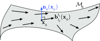
Figure 2: The normal vector field $\mathbf{n}_{0}(\mathbf{x}_{0})$ of any initial material barrier $\mathcal{M}_{0}$ must be orthogonal to the barrier vector field $\mathbf{b}_{t_{0}}^{t_{1}}(\mathbf{x}_{0})$. Therefore, $\mathcal{M}_{0}$ must be a two-dimensional invariant manifold of the vector field $\mathbf{b}_{t_{0}}^{t_{1}}=\overline{\det\nabla\mathbf{F}_{t_{0}}^{t}\left(\mathbf{F}_{t_{0}}^{t}\right)^{*}\mathbf{h}_{vis}}$.

We conclude that if $s\in\mathbb{R}$ parametrizes the streamlines $\mathbf{x}_{0}(s)$ of $\mathbf{b}_{t_{0}}^{t_{1}}(\mathbf{x}_{0})$ and differentiation with respect to $s$ is denoted by a prime, then any 2D streamsurface (i.e., invariant manifold) of the 3D autonomous differential equation,

$$\mathbf{x}_{0}^{\prime}=\mathbf{b}_{t_{0}}^{t_{1}}(\mathbf{x}_{0}),$$ (21)

is a diffusive transport barrier candidate. For this reason, we refer to eq. (21) as the barrier equation, and to $\mathbf{b}_{t_{0}}^{t_{1}}(\mathbf{x}_{0})$ as the corresponding barrier vector field. By the objectivity of the vector field $\mathbf{b}_{t_{0}}^{t_{1}}(\mathbf{x}_{0})$, the barrier equation (21) is objective. Indeed, after a frame change of the form (3), we obtain the transformed barrier equation $\mathbf{Q}(t_{0})\tilde{\mathbf{y}}_{0}^{\prime}=\mathbf{Q}(t_{0})\tilde{\mathbf{b}}_{t_{0}}^{t}(\mathbf{y}_{0})$, which gives $\tilde{\mathbf{y}}_{0}^{\prime}=\tilde{\mathbf{b}}_{t_{0}}^{t}(\mathbf{y}_{0})$.

Any smooth curve of initial conditions for the differential equation (21), however, generates a 2D streamsurface of trajectories for eq. (3). Of these infinitely many barrier candidates, we would like to find only the barrier surfaces with an observable impact on the transport of $\mathbf{f}$. To this end, we formally define active transport barriers as follows:

Definition 2.

A diffusive transport barrier for the vector field $\mathbf{f}$ over the time interval $[t_{0},t_{1}]$ is a material surface $\mathcal{B}(t)\subset U$ whose initial position $\mathcal{B}_{0}=\mathcal{B}(t_{0})$ is a structurally stable (i.e., persistent under small, smooth perturbations of $\mathbf{u}$), 2D invariant manifold of the autonomous dynamical system (21).

The required dimensionality of $\mathcal{B}(t)$ ensures that it divides locally the space into two 3D regions with minimal diffusive transport between them. The required structural stability of $\mathcal{B}(t)$ ensures that conclusions reached about transport barriers for one specific velocity field $\mathbf{u}$ remain valid under small perturbations of $\mathbf{u}$ as well (see Guckenheimer & Holmes 1983).

While a general classification of structurally stable invariant manifolds in 3D dynamical systems is not available, structurally stable 2D surfaces in 3D, steady volume-preserving flows are known to be families of neutrally stable 2D tori, 2D stable and unstable manifolds of structurally stable fixed points or of structurally stable periodic orbits (see, e.g., MacKay 1994). Such structurally stable fixed points and periodic orbits are either hyperbolic or are contained in no-slip boundaries and become hyperbolic after a rescaling of time (Surana, Grunberg & Haller 2006). In view of these results, the three possible active barrier geometries for volume-preserving barrier equations in 3D are shown in Fig. 3.

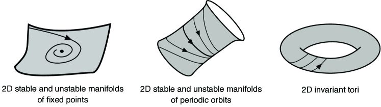
Figure 3: Possible geometries of material barriers to diffusive transport. Curves with arrows indicate qualitative sketches of trajectories of the barrier equation (21), for which these barriers are structurally stable, two-dimensional invariant manifolds.

As we shall see, the barrier-equations for momentum, angular momentum and vorticity are always volume-preserving for incompressible flows and hence the possible active barriers fall in the three categories shown in Fig. 3. For compressible flows, the barrier equations are generally not volume-preserving but the three barrier geometries shown in Fig. 3 nevertheless frequently arise in such flows as well. Invariant tori in compressible barrier equations, however, must necessarily be isolated attractors or repellers, as opposed to members of neutrally stable torus families.

5 Eulerian active barriers

Our treatment of active barriers has so far been fundamentally Lagrangian, targeting material surfaces that render the diffusive transport functional $\psi_{t_{0}}^{t_{1}}$ zero. Taking the $t_{1}\to t_{0}\equiv t$ limit in our arguments yields that instantaneous diffusive-flux minimizing surfaces (Eulerian active barriers) are structurally stable, 2D invariant manifolds of the instantaneous barrier equation

$$\mathbf{x}^{\prime} =\mathbf{b}_{t}^{t}(\mathbf{x})=\mathbf{h}_{vis}\left(\mathbf{x},t,\mathbf{u}(\mathbf{x},t),\mathbf{f}(\mathbf{x},t),\mathbf{T}_{vis}(\mathbf{x},t)\right),$$ (22)

with $t$ fixed and prime still denoting differentiation with respect to the dummy parameter $s$.

The active barriers extracted from (22) can be calculated from instantaneous velocity data without Lagrangian advection, yet they inherit the objectivity of Lagrangian barriers. These instantaneous barriers, therefore, extend the notion of objective Eulerian coherent structures (Serra & Haller 2016) and instantaneous passive diffusion barriers (Haller, Karrasch & Kogelbauer 2018, 2019) to the transport of active vector fields.

6 Active barrier equations for momentum and vorticity

We now derive material barrier equations for different active vector fields. In each case, the instantaneous limits of these equations can directly be obtained by replacing $\mathbf{F}_{t_{0}}^{t}$ with the identity map and omitting the averaging operation in time.

6.1 Barriers to linear momentum transport

Setting $\mathbf{f}:=\rho\mathbf{u}$, we can rewrite eq. (1) as

$$\frac{D\mathbf{f}}{Dt}=\bm{\nabla}\cdot\mathbf{T}_{vis}-\bm{\nabla}p+\mathbf{q}-\frac{D\rho}{Dt}\mathbf{u},$$ (23)

and hence obtain

$$\mathbf{h}_{vis}=\bm{\nabla}\cdot\mathbf{T}_{vis},\qquad\mathbf{h}_{nonvis}=-\bm{\nabla}p+\mathbf{q}-\frac{D\rho}{Dt}\mathbf{u},$$ (24)

for the viscous and non-viscous terms in (5). The viscous stress tensor and its divergence are objective (Gurtin, Fried & Anand 2013), and hence the $\mathbf{h}_{vis}$ function in (24) satisfies the objectivity condition (6). Accordingly, the barrier equations (21) and (22) for the diffusive transport of linear momentum become

$$\mathbf{x}_{0}^{\prime} =\overline{\det\nabla\mathbf{F}_{t_{0}}^{t}\left(\mathbf{F}_{t_{0}}^{t}\right)^{*}\left[\bm{\nabla}\cdot\mathbf{T}_{vis}\right]},$$ (25)

$$\mathbf{x}^{\prime} =\bm{\nabla}\cdot\mathbf{T}_{vis}.$$ (26)

Specifically, in the case of incompressible Navier–Stokes flows with kinematic viscosity $\nu$, we have the constitutive law $\bm{\nabla}\cdot\mathbf{T}_{vis}=\nu\rho\Delta\mathbf{u}$ in the general momentum equation (23); we also observe that $\det\nabla\mathbf{F}_{t_{0}}^{t}\equiv 1$ holds by incompressibility. We then obtain the following:

Theorem 3.

For incompressible, uniform-density Navier–Stokes flows, the material and instantaneous barrier equations (25) and (26) for linear momentum take the specific forms

$$\mathbf{x}_{0}^{\prime} =\nu\rho\,\overline{\left(\mathbf{F}_{t_{0}}^{t}\right)^{*}\Delta\mathbf{u}},$$ (27)

$$\mathbf{x}^{\prime} =\nu\rho\,\Delta\mathbf{u}.$$ (28)

Each of the eqs. (27)-(28) defines a 3D, autonomous (or steady) dynamical system with respect to the time-like variable $s\in\mathbb{R}$, and hence can be analyzed via tools developed for steady flows in the chaotic advection literature (Aref et al. 2017). For the purpose of finding active transport barriers, all the relevant information about the unsteadiness of $\mathbf{u}\left(\mathbf{x},t\right)$ over the time interval $\left[t_{0},t_{1}\right]$ is encoded into eq. (27) through the pull-back and the temporal averaging operations. The instantaneous version (28) of these equations only contains the physical time $t$ as a parameter; it is, therefore, also a steady ODE with respect to the variable $s$ parametrizing its streamlines. Both dynamical systems in (27)-(28) are volume-preserving because $\Delta\mathbf{u}$ is divergence-free for incompressible flows. Therefore, the three possible active barrier geometries arising from the analysis of these barrier equations are those shown in Fig. 3.

In order to solve for trajectories of eq. (27) accurately over a domain $U$ with boundary $\partial U$, one must be aware of any special boundary condition that $\mathbf{b}_{t_{0}}^{t_{1}}(\mathbf{x}_{0})$ may have to satisfy along $\partial U$. We assume for simplicity that $\mathbf{u}(\mathbf{x},t)$ is incompressible and $\partial U$ is a no-slip boundary. Then, after projecting the Navier–Stokes equation (1) at a point $\mathbf{x}\in\partial U$ onto a local orthogonal basis $(\mathbf{e}_{1},\mathbf{e}_{2},\mathbf{e}_{3})$, with $\mathbf{e}_{3}$ normal to the wall, we obtain

$$\left(\begin{array}[]{c}0\\ 0\\ 0\end{array}\right)=\nu\left(\begin{array}[]{c}0\\ 0\\ \Delta\mathbf{u}\cdot\mathbf{e}_{3}\end{array}\right)+\left(\begin{array}[]{c}\left(\mathbf{q}-\frac{1}{\rho}\bm{\nabla}p\right)\cdot\mathbf{e}_{1}\\ \left(\mathbf{q}-\frac{1}{\rho}\bm{\nabla}p\right)\cdot\mathbf{e}_{2}\\ \left(\mathbf{q}-\frac{1}{\rho}\bm{\nabla}p\right)\cdot\mathbf{e}_{3}\end{array}\right).$$ (29)

Therefore, if the wall-normal pressure gradient balances out the external body forces along $\partial U$ (as is often assumed in CFD simulations), then $\Delta\mathbf{u}$ satisfies a no-penetration boundary condition along the no-slip boundary $\partial U$, because $\Delta\mathbf{u}\cdot\mathbf{e}_{3}$ must vanish at each boundary point by (29). Given that such a boundary $\partial U$ is invariant under the flow map $\mathbf{F}_{t_{0}}^{t}$, we obtain that the pull-back of $\Delta\mathbf{u}$ under the flow map must also be tangent to the boundary. Consequently, any no-slip boundary $\partial U$ with a vanishing boundary-normal resultant force is an invariant manifold for the barrier equations (27)-(28).

6.2 Barriers to angular momentum transport

To analyze angular momentum barriers, we take the cross product of eq. (1) with a vector $\mathbf{r}=\mathbf{x-\hat{x}}$, where $\mathbf{\hat{x}}\in U$ marks a fixed reference point. Setting then $\mathbf{f}:=\mathbf{r}\times\rho\mathbf{u},$ we obtain an evolution equation for $\mathbf{f}$ in the form

$$\frac{D\mathbf{f}}{Dt}=\left(\mathbf{x-\hat{x}}\right)\times\frac{D\rho}{Dt}\mathbf{u}-\left(\mathbf{x-\hat{x}}\right)\times\bm{\nabla}p+\left(\mathbf{x-\hat{x}}\right)\times\mathbf{\mathbf{q}}+\left(\mathbf{x-\hat{x}}\right)\times\bm{\nabla}\cdot\mathbf{T}_{vis},$$ (30)

implying

$$\mathbf{h}_{vis}=\left(\mathbf{x-\hat{x}}\right)\times\bm{\nabla}\cdot\mathbf{T}_{vis},\qquad\mathbf{h}_{nonvis}=\left(\mathbf{x-\hat{x}}\right)\times\left[-\bm{\nabla}p+\mathbf{q}+\frac{D\rho}{Dt}\mathbf{u}\right],$$ (31)

for the viscous and non-viscous terms in (5). Under a frame-change of the form (3), this $\mathbf{h}_{vis}$ satisfies

$$\mathbf{h}_{vis}=\left(\mathbf{x-\hat{x}}\right)\times\bm{\nabla}\cdot\mathbf{T}_{vis}=\mathbf{Q}(t)\left(\mathbf{y-\hat{y}}\right)\times\mathbf{Q}(t)\tilde{\bm{\nabla}}\cdot\tilde{\mathbf{T}}_{vis}=\left(\mathbf{y-\hat{y}}\right)\times\tilde{\bm{\nabla}}\cdot\tilde{\mathbf{T}}_{vis}=\tilde{\mathbf{h}}_{vis},$$ (32)

where we have used the objectivity of $\bm{\nabla}\cdot\mathbf{T}_{vis}$. We conclude from (32) that the objectivity condition (6) is satisfied for this choice of $\mathbf{f}$, and hence our formulation is applicable. We, therefore, obtain, as in the case of linear momentum, the following result:

Theorem 4.

For incompressible, uniform-density Navier–Stokes flows, the material and instantaneous barrier equations (21) and (22) for angular momentum take the specific form

$$\mathbf{x}_{0}^{\prime} =\nu\rho\,\overline{\left(\mathbf{F}_{t_{0}}^{t}\right)^{*}\left[\left(\mathbf{x-\hat{x}}\right)\times\Delta\mathbf{u}\right]},$$ (33)

$$\mathbf{x}^{\prime} =\nu\rho\,\left(\mathbf{x-\hat{x}}\right)\times\Delta\mathbf{u}.$$ (34)

These equations again define 3D, steady, volume-preserving dynamical systems with respect to the time-like independent variable $s\in\mathbb{R}$. As in the case of barriers to the transport of linear momentum, we find that in the presence of zero boundary-normal resultant force, eq. (30) implies any no-slip boundary $\partial U$ to be an invariant manifold for the two dynamical systems in (33)-(34).

6.3 Barriers to vorticity transport

To obtain the evolution equation for the active vector field $\mathbf{f}:=\bm{\omega}$, we divide eq. (1) by $\rho$, take the curl of both sides and use the relation $\bm{\nabla}\times\bm{\nabla}p=\mathbf{0}$ to obtain the general vorticity transport equation

$$\frac{D\mathbf{f}}{Dt}=\left(\bm{\nabla}\mathbf{u}\right)\mathbf{f}-\left(\bm{\nabla}\cdot\mathbf{u}\right)\mathbf{f}+\frac{1}{\rho^{2}}\bm{\nabla}\rho\times\bm{\nabla}p+\bm{\nabla}\times\left(\frac{1}{\rho}\mathbf{\mathbf{q}}\right)+\nu\bm{\nabla}\times\left(\frac{1}{\rho}\bm{\nabla}\cdot\mathbf{T}_{vis}\right).$$ (35)

Consequently, our general formulation (5) applies with

$$\mathbf{h}_{vis}=\nu\bm{\nabla}\times\left(\frac{1}{\rho}\bm{\nabla}\cdot\mathbf{T}_{vis}\right),\qquad\mathbf{h}_{nonvis}=\left(\bm{\nabla}\mathbf{u}\right)\mathbf{f}-\left(\bm{\nabla}\cdot\mathbf{u}\right)\mathbf{f}+\frac{1}{\rho^{2}}\bm{\nabla}\rho\times\bm{\nabla}p+\bm{\nabla}\times\left(\frac{1}{\rho}\mathbf{\mathbf{q}}\right).$$ (36)

Following the derivation of the transformation formula for vorticity under an observer change (3) (see, e.g., Truesdell & Rajagopal 2009), we obtain that $\mathbf{h}_{vis}=\mathbf{Q}(t)\tilde{\mathbf{h}}_{vis}$. Therefore, the objectivity condition (6) is satisfied for this choice of $\mathbf{f}$, and hence our formulation is applicable. The barrier equations (21) and (22) for diffusive vorticity transport then become

$$\mathbf{x}_{0}^{\prime} =\nu\,\overline{\det\nabla\mathbf{F}_{t_{0}}^{t}\left(\mathbf{F}_{t_{0}}^{t}\right)^{*}\left[\bm{\nabla}\times\left(\frac{1}{\rho}\bm{\nabla}\cdot\mathbf{T}_{vis}\right)\right]},$$ (37)

$$\mathbf{x}^{\prime} =\nu\,\bm{\nabla}\times\left(\frac{\bm{\nabla}\cdot\mathbf{T}_{vis}}{\rho}\right).$$ (38)

Specifically, as in the case of linear and angular momentum barriers, we obtain:

Theorem 5.

For incompressible, uniform-density Navier–Stokes flows, the material and instantaneous barrier equations (25) and (38) for vorticity take the specific form

$$\mathbf{x}_{0}^{\prime} =\nu\,\overline{\left(\mathbf{F}_{t_{0}}^{t}\right)^{*}\Delta\bm{\omega}},$$ (39)

$$\mathbf{x}^{\prime} =\nu\,\Delta\bm{\omega}.$$ (40)

As in the case of the linear and angular momenta, the active barrier equations (39)-(27) define 3D, autonomous, volume-preserving dynamical systems with respect to the time-like, evolutionary variable $s\in\mathbb{R}$, and hence can be analyzed by adopting tools available such equations (see section 8).

As for boundary conditions for trajectories of the equations (39) along a no-slip boundary $\partial U$ in the incompressible case with $\rho_{0}(\mathbf{x})\equiv 1$, the vorticity-transport equation along the wall $\partial U$ takes the form

$$\left(\begin{array}[]{c}\left(\frac{D}{Dt}\bm{\omega}\right)\cdot\mathbf{e}_{1}\\ \left(\frac{D}{Dt}\bm{\omega}\right)\cdot\mathbf{e}_{2}\\ 0\end{array}\right)=\nu\left(\begin{array}[]{c}\bm{\Delta\omega}\cdot\mathbf{e}_{1}\\ \bm{\Delta\omega}\cdot\mathbf{e}_{2}\\ \bm{\Delta\omega}\cdot\mathbf{e}_{3}\end{array}\right)\Delta\bm{\omega}+\left(\begin{array}[]{c}\bm{\nabla\times q}\cdot\mathbf{e}_{1}\\ \bm{\nabla\times q}\cdot\mathbf{e}_{2}\\ \bm{\nabla\times q}\cdot\mathbf{e}_{3}\end{array}\right),$$ (41)

with the vectors $\mathbf{e}_{i}$ defined as in formula (29). Consequently, whenever the curl of non-potential body forces is normal to a no-slip boundary $\partial U$, the vector field $\Delta\bm{\omega}$ satisfies a no-penetration boundary condition along $\partial U$, given that $\bm{\Delta\omega}\cdot\mathbf{e}_{3}$ must then vanish by (41). As we have already noted in relation to formula (29), this in turn implies that $\partial U$ is an invariant manifold for the two flows in eqs. (39)-(40).

7 Active transport barriers in special classes of flows

In order to illustrate the feasibility of the active barriers we have constructed, we now identify them in classes of explicit Navier–Stokes solutions, with the details of the calculations relegated to Appendices C and D.

7.1 2D Navier–Stokes flows viewed as 3D Navier–Stokes flows with symmetry

We define the planar variable $\bm{\hat{\mathbf{x}}}=\left(x_{1},x_{2}\right)\in\mathbb{R}^{2}$ and assume that a solution of the 3D incompressible Navier–Stokes equation is of the form

$$\mathbf{u}(\mathbf{x},t)=\left(\hat{\mathbf{u}}(\hat{\mathbf{x}},t),w(\hat{\mathbf{x}},t)\right),\quad p(\mathbf{x},t)=p(\hat{\mathbf{x}},t),\qquad\mathbf{x}=\left(\bm{\hat{\mathbf{x}}},x_{3}\right)\in\mathbb{R}^{3},$$ (42)

with the two-dimensional velocity field $\hat{\mathbf{u}}(\hat{\mathbf{x}},t)$ and the scalar functions $w(\hat{\mathbf{x}},t)$ and $p(\hat{\mathbf{x}},t)$ (see, e.g., Majda & Bertozzi 2002). Under this 2D-symmetry ansatz, substitution of $\mathbf{u}$ and $p$ into the 3D Navier–Stokes equation gives

$$\partial_{t}\mathbf{\hat{\mathbf{u}}}+\left(\bm{\nabla}_{\mathbf{\hat{\mathbf{x}}}}\hat{\mathbf{u}}\right)\hat{\mathbf{u}} =-\frac{1}{\rho}\bm{\nabla}_{\mathbf{\hat{\mathbf{x}}}}p+\nu\Delta_{\hat{\mathbf{x}}}\hat{\mathbf{u}},$$ (43)

$$\partial_{t}w+\bm{\nabla}_{\mathbf{\hat{\mathbf{x}}}}w\cdot\hat{\mathbf{u}} =\nu\Delta_{\hat{\mathbf{x}}}w,$$ (44)

with the subscript $\hat{\mathbf{x}}$ referring to the 2D version of the differential operators involved. Therefore, the symmetry ansatz (42) for a 3D Navier-Stokes solution is valid if $w(\hat{\mathbf{x}},t)$ is chosen as a solution of the advection-diffusion equation appearing in (44). This advection-diffusion equation, however, coincides with the 2D vorticity transport equation, which is solved by

$$w(\bm{\hat{\mathbf{x}}},t)=\hat{\omega}(\bm{\hat{\mathbf{x}}},t),$$ (45)

with $\hat{\omega}(\bm{\hat{\mathbf{x}}},t)$ denoting the scalar vorticity field of the 2D Navier–Stokes solution $\hat{\mathbf{u}}(\bm{\hat{\mathbf{x}}},t)$. In the following, we will choose the third component of $\mathbf{u}$ as in eq. (45) and use the notation

$$\mathbf{J}=\left(\begin{array}[]{rc}0&1\\ -1&0\end{array}\right)$$ (46)

for the two-dimensional canonical symplectic matrix $\mathbf{J}$. With this notation, we obtain the following results on active barriers to momentum transport in eq. (42).

Theorem 6.

For 2D incompressible, uniform-density Navier–Stokes flows, the material and instantaneous barrier equations (27) and (28) for linear momentum are autonomous Hamiltonian systems of the form

$$\hat{\mathbf{x}}_{0}^{\prime} =\nu\rho\,\mathbf{J}\bm{\nabla}_{0}\,\overline{\hat{\omega}\left(\hat{\mathbf{F}}_{t_{0}}^{t}\left(\hat{\mathbf{x}}_{0}\right),t\right)},$$ (47)

$$\hat{\mathbf{x}}^{\prime} =\nu\rho\,\mathbf{J}\bm{\nabla}\,\hat{\omega}\left(\hat{\mathbf{x}},t\right),$$ (48)

respectively. Therefore, time-$t_{0}$ positions of material active barriers to linear momentum transport in these flows are structurally stable level curves of the time-averaged Lagrangian vorticity $\overline{\hat{\omega}\left(\hat{\mathbf{F}}_{t_{0}}^{t}\left(\mathbf{\hat{x}}_{0}\right),t\right)}$ viewed as a Hamiltonian. Similarly, instantaneous active barriers to linear momentum transport at time $t$ are structurally stable level curves of the vorticity $\hat{\omega}(\bm{\hat{\mathbf{x}}},t)$.

Proof 7.1.

See Appendix C.

While streamlines in general are not objective, the streamlines of the vorticity $\hat{\omega}(\bm{\hat{\mathbf{x}}},t)$ are Eulerian-objective and streamlines of the time-averaged Lagrangian vorticity $\overline{\hat{\omega}\left(\hat{\mathbf{F}}_{t_{0}}^{t}\left(\mathbf{\hat{x}}_{0}\right),t\right)}$ are Lagrangian-objective (see Ogden 1984). This is consistent with the more general result established in eq. (18) for the objectivity of all active barriers.

Active barriers to vorticity transport in (42) also turn out to be trajectories of autonomous Hamiltonian systems. To state this result, we will use the notation

$$\delta\hat{\omega}\left(\hat{\mathbf{x}}_{0},t_{0},t_{1}\right):=\hat{\omega}\left(\hat{\mathbf{F}}_{t_{0}}^{t_{1}}\left(\hat{\mathbf{x}}_{0}\right),t_{1}\right)-\hat{\omega}\left(\hat{\mathbf{x}}_{0},t_{0}\right)$$ (49)

for the Lagrangian vorticity-change function along trajectories over the time interval $[t_{0},t_{1}]$.

Theorem 7.

For 2D incompressible, uniform-density Navier–Stokes flows, the material and instantaneous barrier equations (39) and (40) for linear momentum are autonomous Hamiltonian systems of the form

$$\hat{\mathbf{x}}_{0}^{\prime} =\frac{\nu}{t_{1}-t_{0}}\,\mathbf{J}\bm{\nabla}_{0}\,\delta\hat{\omega}\left(\hat{\mathbf{x}}_{0},t_{0},t_{1}\right),$$ (50)

$$\hat{\mathbf{x}}^{\prime} =\nu\,\mathbf{J}\bm{\nabla}\frac{D}{Dt}\hat{\omega}\left(\hat{\mathbf{x}},t\right),$$ (51)

respectively. Therefore, time-$t_{0}$ positions of material active barriers to linear momentum transport in these flows are structurally stable level curves of the Lagrangian vorticity-change function $\delta\hat{\omega}\left(\hat{\mathbf{x}}_{0},t_{0},t_{1}\right)$ viewed as a Hamiltonian. Similarly, instantaneous active barriers to linear momentum transport at time $t$ are structurally stable level curves of the material derivative $\frac{D}{Dt}\hat{\omega}\left(\hat{\mathbf{x}},t\right)$, or equivalently, of the vorticity Laplacian $\Delta\hat{\omega}\left(\hat{\mathbf{x}},t\right).$

Proof 7.2.

See Appendix C.

While vorticity is not objective, the level curves of the Lagrangian vorticity change $\delta\hat{\omega}\left(\hat{\mathbf{x}}_{0},t_{0},t_{1}\right)$ is objective. This follows directly from the objectivity of the barrier equations that we have generally established, but can also be verified directly using the definition of objectivity.

Remark 8.

By Theorems 6-7, outermost members of nested families of closed level curves of $\overline{\hat{\omega}\left(\hat{\mathbf{F}}_{t_{0}}^{t}\left(\mathbf{\hat{x}}_{0}\right),t\right)}$ or $\delta\hat{\omega}\left(\hat{\mathbf{x}}_{0},t_{0},t_{1}\right)$ can be used to define coherent material vortex boundaries. These are constructed as maximal barriers to momentum or vorticity transport, depending on whether one isolates coherent vortices based on their role in momentum- or vorticity-transport, respectively. Similarly, to locate instantaneous Eulerian vortex boundaries, one identifies outermost members of nested families of closed level curves of $\hat{\omega}(\bm{\hat{\mathbf{x}}},t)$ or $\frac{D}{Dt}\hat{\omega}\left(\hat{\mathbf{x}},t\right)$, respectively. These outermost contours give a clear conceptual meaning to vortex boundaries from an active transport perspective, but their identification from numerical data tends to be a sensitive process. Instead, active-transport-minimizing material and instantaneous vortex boundaries can simply be visualized via LCS-detection tools adopted to their appropriate 2D, steady barrier equations (47)-(48) and (50)-(51) (see section 8).

Example 7.3.

We consider the spatially doubly-periodic Navier–Stokes flow family described by Majda & Bertozzi (2002) in the form

$$\hat{\mathbf{u}}(\hat{\mathbf{x}},t) =e^{-4\pi^{2}\ell\nu t}\hat{\mathbf{u}}_{0}(\hat{\mathbf{x}}),\quad p(\hat{\mathbf{x}},t)=e^{-4\pi^{2}\ell\nu t}p_{0}(\hat{\mathbf{x}}),$$ (52)

$$\hat{\mathbf{u}}_{0}(\hat{\mathbf{x}}) =\sum_{\left|\mathbf{k}\right|^{2}=\ell}\left(\begin{array}[]{c}a_{\mathbf{k}}k_{2}\sin\left(2\pi\mathbf{k}\cdot\hat{\mathbf{x}}\right)-b_{\mathbf{k}}k_{2}\cos\left(2\pi\mathbf{k}\cdot\hat{\mathbf{x}}\right)\\ -a_{\mathbf{k}}k_{1}\sin\left(2\pi\mathbf{k}\cdot\hat{\mathbf{x}}\right)+b_{\mathbf{k}}k_{1}\cos\left(2\pi\mathbf{k}\cdot\hat{\mathbf{x}}\right)\end{array}\right),$$ (55)

where $\hat{\mathbf{u}}_{0}(\hat{\mathbf{x}})$ and $p_{0}(\hat{\mathbf{x}})$ solve the steady planar Euler equation for some positive integer $\ell$. In that case, we have

$$\Delta\mathbf{u} =\left(\begin{array}[]{c}\Delta_{\hat{\mathbf{x}}}\hat{\mathbf{u}}\\ \Delta_{\hat{\mathbf{x}}}\hat{\omega}\end{array}\right)=\left(\begin{array}[]{c}-4\pi^{2}\ell e^{-4\pi^{2}\ell\nu t}\hat{\mathbf{u}}_{0}(\hat{\mathbf{x}})\\ \Delta_{\hat{\mathbf{x}}}\hat{\omega}(\hat{\mathbf{x}},t)\end{array}\right).$$ (60)

One can verify by direct substitution that $e^{-4\pi^{2}\ell\nu t}\hat{\mathbf{u}}_{0}\left(\hat{\mathbf{F}}_{t_{0}}^{t}\left(\mathbf{\hat{\mathbf{x}}}_{0}\right)\right)$ is a solution of the equation of variations $\dot{\bm{\xi}}=e^{-4\pi^{2}\ell\nu t}\bm{\nabla}_{\mathbf{\hat{\mathbf{x}}}}\hat{\mathbf{u}}_{0}(\hat{\mathbf{x}}(t))\bm{\xi}$ (whose fundamental matrix solution is $\nabla_{\hat{\mathbf{x}}_{0}}\mathbf{\hat{F}}_{t_{0}}^{t}\left(\mathbf{x}_{0}\right)$) for the differential equation $\dot{\mathbf{x}}=e^{-4\pi^{2}\ell\nu t}\hat{\mathbf{u}}_{0}(\hat{\mathbf{x}})$. As a consequence, we have

$$\left[\bm{\nabla}_{\mathbf{\hat{\mathbf{x}}}_{0}}\hat{\mathbf{F}}_{t_{0}}^{t}\left(\mathbf{\hat{\mathbf{x}}}_{0}\right)\right]^{-1}e^{-4\pi^{2}\ell\nu t}\hat{\mathbf{u}}_{0}\left(\hat{\mathbf{F}}_{t_{0}}^{t}\left(\mathbf{\hat{\mathbf{x}}}_{0}\right)\right)=e^{-4\pi^{2}\ell\nu t_{0}}\hat{\mathbf{u}}_{0}\left(\mathbf{\hat{\mathbf{x}}}_{0}\right),$$

and hence, by Theorem 6, the material and instantaneous barrier equations for linear momentum take the specific form

$$\hat{\mathbf{x}}_{0}^{\prime} =\nu\rho e^{-4\pi^{2}\ell\nu t_{0}}\hat{\mathbf{u}}_{0}\left(\mathbf{\hat{\mathbf{x}}}_{0}\right),$$

$$x_{03}^{\prime} =\nu\rho A(\mathbf{\hat{\mathbf{x}}}_{0},t_{1},t_{0}),$$ (61)

$$\hat{\mathbf{x}}^{\prime} =\nu\rho e^{-4\pi^{2}\ell\nu t}\hat{\mathbf{u}}_{0}\left(\mathbf{\hat{\mathbf{x}}}\right),$$

$$x_{3}^{\prime} =\nu\rho A(\mathbf{\hat{\mathbf{x}}},t,t),$$

for an appropriate function $A(\mathbf{\hat{\mathbf{x}}}_{0},t_{1},t_{0})$. Therefore, both material and instantaneous barriers to linear momentum transport in the 2D Navier–Stokes flow family in eq. (52) are structurally stable streamlines of the steady velocity field $\hat{\mathbf{u}}_{0}\left(\mathbf{\hat{\mathbf{x}}}_{0}\right)$.

As for vorticity barriers in this example, note that

$$\hat{\omega} =\partial_{x_{1}}u_{2}-\partial_{x_{2}}u_{1}=-2\pi\ell e^{-4\pi^{2}\ell\nu t}\hat{\omega}_{0},$$ (62)

$$\hat{\omega}_{0}\left(\mathbf{\hat{\mathbf{x}}}\right) =\sum_{\left|\mathbf{k}\right|^{2}=\ell}a_{\mathbf{k}}\cos\left(2\pi\mathbf{k}\cdot\hat{\mathbf{x}}\right)+b_{\mathbf{k}}\sin\left(2\pi\mathbf{k}\cdot\hat{\mathbf{x}}\right).$$ (63)

As the steady part of the vorticity field solves the steady planar Euler equation, trajectories of $\hat{\mathbf{u}}(\hat{\mathbf{x}},t)$ remain confined to the steady streamlines of $\hat{\mathbf{u}}_{0}\left(\mathbf{\hat{\mathbf{x}}}_{0}\right)$. Since these trajectories also conserve the vorticity $\hat{\omega}_{0}$ of the inviscid limit of the flow, the change in vorticity $\hat{\omega}\left(\hat{\mathbf{x}},t\right)$ along trajectories of $\hat{\mathbf{u}}(\hat{\mathbf{x}},t)$ can be written as

$$\delta\hat{\omega}\left(\hat{\mathbf{x}}_{0},t_{0},t_{1}\right)=-2\pi\ell\left(e^{-4\pi^{2}\ell\nu t_{1}}-e^{-4\pi^{2}\ell\nu t_{0}}\right)\hat{\omega}_{0}\left(\mathbf{\hat{\mathbf{x}}}_{0}\right).$$ (64)

Therefore, level curves of the vorticity change along trajectories coincide with those of the inviscid vorticity $\hat{\omega}_{0}\left(\mathbf{\hat{\mathbf{x}}}_{0}\right)$, which are in turn just the streamlines of $\hat{\mathbf{u}}_{0}\left(\mathbf{\hat{\mathbf{x}}}_{0}\right)$. Finally, we have

$$\Delta\hat{\omega}\left(\hat{\mathbf{x}},t\right)=8\pi^{3}\ell^{2}e^{-4\pi^{2}\ell\nu t}\hat{\omega}_{0}\left(\mathbf{\hat{\mathbf{x}}}\right),$$ (65)

and hence the level curves of $\Delta\hat{\omega}\left(\hat{\mathbf{x}},t\right)$ also coincide with those of $\hat{\mathbf{u}}_{0}\left(\mathbf{\hat{\mathbf{x}}}\right)$.

We conclude that both material and instantaneous active barriers to vorticity and linear momentum transport coincide with the streamlines of $\hat{\mathbf{u}}_{0}\left(\mathbf{\hat{\mathbf{x}}}_{0}\right)$. In particular, we obtain the correct active barrier distributions that we inferred for our motivational 2D channel-flow example in Fig. 1 (see (91) in Appendix A), which is part of the solution family (52). Importantly, we obtain the same frame-indifferent conclusion about active barriers from any finite-time (or even instantaneous) analysis of the velocity field (52) .

7.2 Directionally steady Beltrami flows

Virtually all explicitly known, unsteady solutions of the 3D incompressible Navier–Stokes equations satisfy the strong Beltrami property

$$\bm{\mathbf{\omega}}(\mathbf{x},t)=k(t)\mathbf{u}(\mathbf{x},t)$$ (66)

for some scalar function $k(t)$ (see Majda & Bertozzi 2002). By definition, for any such incompressible strong Beltrami flow, we obtain

$$\Delta\bm{\omega} =\bm{\nabla}\left(\bm{\nabla}\cdot\bm{\omega}\right)-\bm{\nabla}\times\left(\bm{\nabla}\times\bm{\omega}\right)=-k^{3}\mathbf{u},$$

$$\Delta\mathbf{u} =\frac{1}{k}\Delta\bm{\omega}=-k^{2}\mathbf{u}.$$ (67)

Recall that if a steady Euler flow is non-Beltrami, then it is integrable (Arnold & Keshin 1998). Therefore, only velocity field satisfying the Beltrami property can generate complicated particle dynamics in steady, inviscid flows.

We call an unsteady strong Beltrami flow with velocity field $\mathbf{u}(\mathbf{x},t)$ a directionally steady Beltrami flow if

$$\mathbf{u}(\mathbf{x},t)=\alpha(t)\mathbf{u}_{0}(\mathbf{x}),\quad\bm{\mathbf{\mathbf{\omega}}}\left(\mathbf{x},t\right)=\bm{\nabla}\times\mathbf{u}(\mathbf{x},t)=k(t)\alpha(t)\mathbf{u}_{0}\left(\mathbf{x}\right)$$ (68)

hold for some continuously differentiable scalar function $\alpha(t)$. Note that any steady strong Beltrami flow $\mathbf{u}_{0}(\mathbf{x})$ (which necessarily admits $k(t)\equiv k=const.)$ solves the steady Euler equation and generates a directionally steady Beltrami solution $\mathbf{u}(\mathbf{x},t)=\exp\left(-\nu k^{2}t\right)\mathbf{u}_{0}(\mathbf{x})$ for the unsteady Navier–Stokes equation under conservative forcing (Majda and Bertozzi 2002).

For all directionally steady Beltrami flows, we obtain the following simple result on active transport barriers:

Theorem 9.

Both material and instantaneous active barriers to the diffusive transport of linear momentum and vorticity in directionally steady Beltrami flows coincide exactly with structurally stable, 2D invariant manifolds of the steady component $\mathbf{u}_{0}(\mathbf{x})$ of the velocity field. These in turn coincide with 2D invariant manifolds of $\mathbf{u}(\mathbf{x},t)$ defined in (142).

Proof 7.4.

See Appendix D.

Theorem 9 shows that invariant manifolds for the Lagrangian particle motion in directionally steady Beltrami flows coincide with material and instantaneous active barriers to linear momentum and vorticity transport. This agrees with one’s intuition: observed mass-transport barriers in these flows are expected to coincide with barriers to vorticity and momentum transport, given that momentum and vorticity are scalar multiples of each other. Remarkably, as in the case of 2D flows analyzed in the previous section, the exact barriers emerge from our analysis independently of the choice of the finite-time interval $[t_{0},t_{1}]$, including the case of instantaneous extraction with $t_{0}=t_{1}$.

Remark 10.

In view of Theorem 9, when viewed as transport barriers to momentum and vorticity, both Lagrangian and Eulerian coherent vortex boundaries in directionally steady Beltrami flows coincide with outermost members of nested families of invariant tori identified form purely advective mixing studies (see, e.g., Dombre et al. 1986 and Haller 2001). This is in line with the expectation we stated earlier that the outermost members of a family of non-filamenting, closed material surfaces will also be outermost barriers to diffusive transport.

Example 7.5.

Examples of directionally steady Beltrami flows include the Navier-Stokes flow family (Ethier & Steinman 1994)

$$\mathbf{u}(\mathbf{x},t)=e^{-\nu d^{2}t}\mathbf{u}_{0}(\mathbf{x}),\qquad\mathbf{u}_{0}(\mathbf{x})=-a\left(\begin{array}[]{c}e^{ax_{1}}\sin\left(ax_{2}\pm dx_{3})+e^{ax_{3}}\cos\left(ax_{1}\pm dx_{2}\right)\right)\\ e^{ax_{2}}\sin\left(ax_{3}\pm dx_{1})+e^{ax_{1}}\cos\left(ax_{2}\pm dx_{3}\right)\right)\\ e^{ax_{3}}\sin\left(ax_{1}\pm dx_{2})+e^{ax_{2}}\cos\left(ax_{3}\pm dx_{1}\right)\right)\end{array}\right),$$ (69)

and the viscous, unsteady version of the classic ABC flow $\mathbf{u}_{0}(\mathbf{x})$ (Dombre et al. 1986), given by

$$\mathbf{u}(\mathbf{x},t)=e^{-\nu t}\mathbf{u}_{0}(\mathbf{x}),\qquad\mathbf{u}_{0}(\mathbf{x})=\left(\begin{array}[]{c}A\sin x_{3}+C\cos x_{2}\\ B\sin x_{1}+A\cos x_{3}\\ C\sin x_{2}+B\cos x_{1}\end{array}\right).$$ (70)

All lengths in these examples are non-dimensional. Further examples of 3D, unsteady but directionally steady Beltrami solutions are derived by Barbato, Berselli & Grisanti (2007) and Antuono (2020).

For all these flows, Theorem 9 guarantees that all material and instantaneous active barriers to diffusive momentum and vorticity transport coincide with structurally stable, 2D invariant manifolds of the flow generated by the steady velocity field $\mathbf{u}_{0}(\mathbf{x})$. Such manifolds can be captured via their intersections with Poincaré sections, with these intersections appearing as invariant curves of the associated Poincaré map, as first illustrated by Dombre et al. (1986) for one cross-section of the ABC flow. A more complete set of Poincaré maps along three orthogonal planes is shown in the right subplot Fig. 4, which reveals several families of 2D invariant tori, appearing as spatially periodic cylinders.

As discussed in Remark 10, these torus families form objectively defined coherent vortices, with each torus acting as an internal barriers to both momentum- and vorticity-transport within the vortex. Outermost members of these torus families provide objective, active-transport-based coherent vortex boundaries. By their invariance under the flow map, they remain perfectly coherent under advection. For comparison, we also show in Fig. 4 other common Eulerian diagnostics applied to this flow: sectional streamlines (computed from velocities projected onto the three faces of the cube at time $t=0$ ); vorticity levels for $\mathbf{u}(\mathbf{x},t)$ at $t=0$; and levels of the parameter $Q=\left|\bm{W}\right|^{2}-\left|\mathbf{S}\right|^{2}$ at $t=0$, with the spin tensor $\mathbf{W}$ and the rate-of-strain tensor $\mathbf{S}$ defined as

$$\mathbf{W}=\frac{1}{2}\left[\bm{\nabla}\mathbf{u}-\left(\bm{\nabla}\mathbf{u}\right)^{T}\right],\quad\mathbf{S}=\frac{1}{2}\left[\bm{\nabla}\mathbf{u}+\left(\bm{\nabla}\mathbf{u}\right)^{T}\right].$$ (71)

The $Q>0$ region is often used to define vortices, and hence the white level sets are considered vortex boundaries by the $Q$-criterion of Hunt et al. (1988). The structures appearing in the latter three plots change under an observer change and do not remain invariant under advection by the flow map.

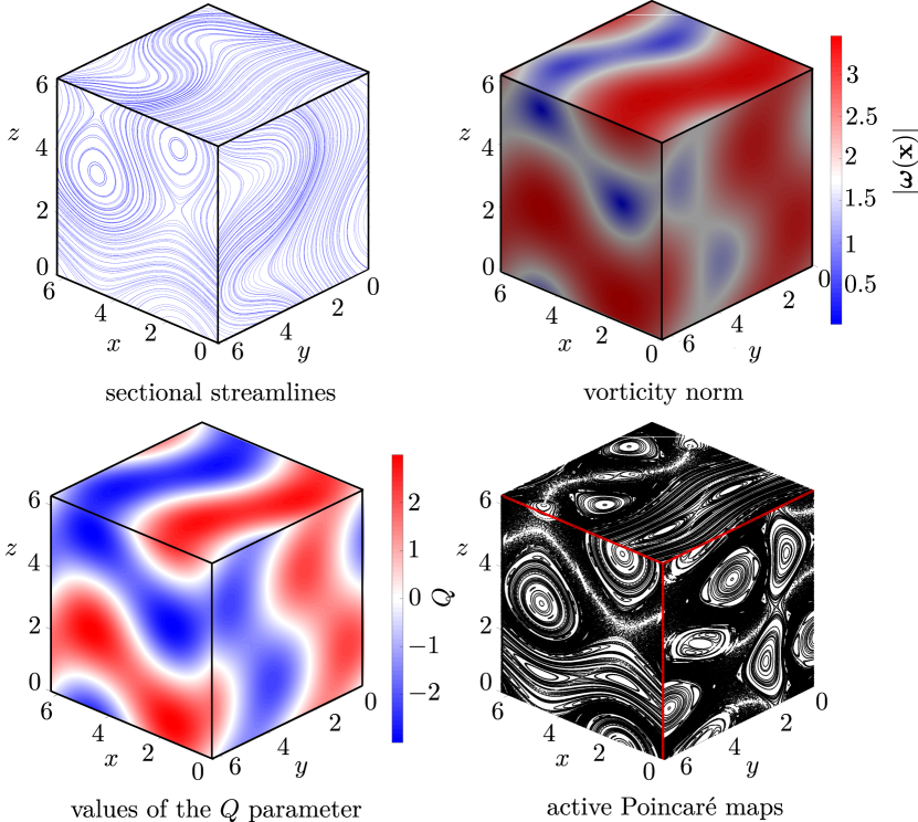
Figure 4: Three nonobjective diagnostics (sectional streamline plots, the vorticity norm and the $Q$-parameter) for the unsteady ABC flow (70) with $A=\sqrt{3}$, $B=\sqrt{2}$ and $C=1$, at time $t=0$. All three plots remain the same for all times, because the velocity field is directionally steady. Also shown are three objective, active Poincaré maps computed for the associated barrier equations. The Lagrangian and Eulerian barrier equations for this flow are given by $\mathbf{x}_{0}^{\prime}=\mathbf{u}_{0}\left(\mathbf{x}_{0}\right)$ by Theorem 9, both for momentum and vorticity. Black dots on the active Poincaré sections indicate repeated return locations of barrier trajectories launched from the same section. Intersections of 2D, toroidal transport barriers with the three Poincaré sections are visible as invariant curves of these Poincaré maps. Outermost members of these torus families define objective coherent vortex boundaries.

Further studies revealing the same invariant manifolds in the steady ABC flow using finite-time Lyapunov exponents (FTLE) and the polar rotation angle (PRA) were given by Haller (2001) and Farazmand & Haller (2016), each emphasizing different classes of barriers from the complete collection revealed in Fig. 4. The FTLE and the PRA are generally usable structure detection tools along any cross section of an unsteady flow, whereas Poincaré maps are only defined for trajectories returning to the same cross section of a steady or time-periodic flow. In the next section, we will also show the passive FTLE and PRA plots computed for the ABC flow (70), as well as active versions of the FTLE and PRA applied to the barrier equations of the ABC flow over the same time interval.

8 Practical implementation of active barrier identification

Here we discuss the computation of the barrier equations for momentum and vorticity from velocity data sets. In addition, we introduce dynamically active versions of three simple LCS techniques that can be used to extract active transport barrier surfaces. While these LCS diagnostics enable a quick visualization of active barriers in an objective fashion, the more advanced LCS methods we cited in the Introduction are also directly applicable to the barrier equations.

8.1 Computation from highly resolved numerical data

All applications of our main results in Theorems 3-5 require the analysis of the associated 3D autonomous, divergence-free dynamical systems that depend on the Laplacian of $\mathbf{u}(\mathbf{x},t)$ for momentum-transport barriers, or on the Laplacian of $\bm{\omega}\left(\mathbf{x},t\right)$ for vorticity-transport barriers. In direct numerical simulations (DNS) of the Navier–Stokes equation, the required Laplacians can be computed spectrally with high accuracy, as our numerical results in Section 9.2 will illustrate. With these Laplacians at hand, one proceeds to find invariant manifolds of the barrier equations in Theorems 3-5, which invariably involves computing trajectories of these equations. In generating these trajectories numerically, it is usually helpful to omit the (small) viscosity $\nu$ from the right-hand sides of the barrier equations to speed up the simulation. This omission of $\nu$ is equivalent to a rescaling of the time-like variable $s$ in the barrier equations, which does not alter the trajectories of these autonomous differential equations.

For 2D incompressible Navier–Stokes flows, Theorems 6-7 show the relevant barrier equations to be computed. The right-hand-sides of these equations are autonomous Hamiltonian vector fields whose trajectories coincide with the level curves of the corresponding Hamiltonians. Strictly speaking, therefore, the numerical solution of these barrier equations can be avoided by simply plotting the level curves of their Hamiltonians, which can be computed by finite-differencing the velocity field (but see also Remark 8 in section 7.1).

8.2 Computation from experimental or lower-resolved numerical data

Taking second and third spatial derivatives of a velocity field obtained from an already finalized numerical simulation or experiment is challenging. An alternative is to work with the original material derivatives arising in our definition of active transport, rather than with the Laplacians of the velocity and the vorticity. More specifically, if we let $\mathbf{a}(\mathbf{x},t)=\frac{D\mathbf{u}}{Dt}(\mathbf{x},t)$ denote the Lagrangian particle acceleration along fluid trajectories, then using the general momentum equation (1), the active barrier equations (25) and (26) for the linear momentum can be rewritten as

$$\mathbf{x}_{0}^{\prime} =\overline{\det\nabla\mathbf{F}_{t_{0}}^{t}\left(\mathbf{F}_{t_{0}}^{t}\right)^{*}\left[\rho\mathbf{a}+\bm{\nabla}p-\mathbf{q}\right]},$$ (72)

$$\mathbf{x}^{\prime} =\rho\mathbf{a}+\bm{\nabla}p-\mathbf{q}.$$ (73)

These equations involve the Lagrangian acceleration, $\mathbf{a}(\mathbf{x},t)$, which can be obtained from high-resolution numerical or experimental data via the temporal differentiation of the velocity vector along trajectories.

Similarly, the most general active barrier equations (37)-(38) for vorticity can be rewritten as

$$\mathbf{x}_{0}^{\prime} =\overline{\det\nabla\mathbf{F}_{t_{0}}^{t}\left(\mathbf{F}_{t_{0}}^{t}\right)^{*}\bm{\nabla}\times\left[\mathbf{a}+\frac{1}{\rho}\left(\bm{\nabla}p-\mathbf{q}\right)\right]},$$ (74)

$$\mathbf{x}^{\prime} =\bm{\nabla}\times\left[\mathbf{a}+\frac{1}{\rho}\left(\bm{\nabla}p-\mathbf{q}\right)\right].$$ (75)

In particular, for incompressible, constant density, Newtonian fluids subject only to potential body forces, the material and instantaneous barrier equations for vorticity in (74)-(75) simplify to

$$\mathbf{x}_{0}^{\prime} =\overline{\left(\mathbf{F}_{t_{0}}^{t}\right)^{*}\bm{\nabla}\times\mathbf{a}},$$ (76)

$$\mathbf{x}^{\prime} =\bm{\nabla}\times\mathbf{a},$$ (77)

given that $\bm{\nabla}\times\left[\frac{1}{\rho}\left(\bm{\nabla}p-\mathbf{q}\right)\right]=\frac{1}{\rho}\bm{\nabla}\times\left[\bm{\nabla}p-\mathbf{q}\right]\equiv\mathbf{0}$ holds for such flows.

8.3 Passive vs. active Poincaré maps

Passive Poincaré maps for 3D steady flows map initial conditions of trajectories launched from a selected 2D section to their first return to the section, if such a return exists. We refer to a Poincaré map computed for the 3D steady barrier equations (21) or (22) as active Poincaré map (see Fig. 4 for an example). This two-dimensional mapping generally does not preserve the standard 2D area, but preserves a general area form, which makes the active Poincaré map a 2D symplectic map (Meiss 1992). One-dimensional invariant curves of 2D symplectic maps satisfy the only available formal definition of advective transport barriers by MacKay, Meiss & Percival (1984), as we noted in the Introduction. Structurally stable invariant curves of 2D symplectic maps include stable and unstable manifolds of hyperbolic fixed points and Kolmogorov–Arnold-Moser (KAM) curves, i.e., nested families of closed curves satisfying non-resonance and twist-conditions (Arnold 1978).

In contrast to active Poincaré maps, the mapping relating subsequent returns of trajectories to a selected section in the general unsteady velocity field $\mathbf{u}(\mathbf{x},t$) is not well-defined as a single Poincaré map. Rather, this map will be different for different initial times $t_{0}$. Therefore, passive Poincaré maps are generally inapplicable to LCS detection in $\mathbf{u}(\mathbf{x},t)$, whereas active Poincaré maps are well-defined on barrier-equation trajectories that return to a cross section. In case they do not, the active versions of the FTLE and PRA fields introduced next provide alternative tools to uncover structurally stable invariant manifolds in the the barrier equations.

8.4 Passive FTLE vs. active FTLE (aFTLE)

We fix a time interval $[t_{0},t_{1}]$ over which we would like to identify LCSs as coherent material surfaces in the advective transport induced by the unsteady velocity field $\mathbf{u}(\mathbf{x},t)$. With the notation of section 2, the right Cauchy–Green strain tensor $\mathbf{C}_{t_{0}}^{t_{1}}\left(\mathbf{x}_{0}\right)$ is defined as

$$\mathbf{C}_{t_{0}}^{t_{1}}\left(\mathbf{x}_{0}\right):=\left[\bm{\nabla}\mathbf{F}_{t_{0}}^{t_{1}}\left(\mathbf{x}_{0}\right)\right]^{T}\bm{\nabla}\mathbf{F}_{t_{0}}^{t_{1}}\left(\mathbf{x}_{0}\right),$$ (78)

with the superscript $T$ referring to the transpose. Then, if $\lambda_{\mathrm{max}}\left(\mathbf{C}_{t_{0}}^{t_{1}}\right)$ denotes the maximal eigenvalues of the symmetric, positive definite tensor $\mathbf{C}_{t_{0}}^{t_{1}}$, then the (passive) FTLE field of $\mathbf{u}(\mathbf{x},t)$ over the $\left[t_{0},t_{1}\right]$ time interval is defined as

$$\mathrm{FTLE}_{t_{0}}^{t_{1}}(\mathbf{x}_{0})=\frac{1}{2\left(t_{1}-t_{0}\right)}\log\lambda_{\mathrm{max}}\left(\mathbf{C}_{t_{0}}^{t_{1}}\left(\mathbf{x}_{0}\right)\right).$$ (79)

Two-dimensional ridges of $\mathrm{FTLE}_{t_{0}}^{t_{1}}(\mathbf{x}_{0})$ are quick indicators of the time $t_{0}$ locations of hyperbolic LCS. They signal locally most repelling material surfaces when $t_{1}>t_{0}$ and locally most attracting material surfaces when $t_{1}<t_{0}$. Valleys of $\mathrm{FTLE}_{t_{0}}^{t_{1}}(\mathbf{x}_{0})$ tend to indicate elliptic (vortical) LCSs, whereas trenches of $\mathrm{FTLE}_{t_{0}}^{t_{1}}(\mathbf{x}_{0})$ signal parabolic (jet-type) LCSs. The minimal and maximal value of $t_{0}$ and $t_{1}$ are governed by the length of the available data and the scales relative to which we wish to determine the LCSs in the flow. The flow-map gradient involved in the definition of $\lambda_{\mathrm{max}}\left(\mathbf{C}_{t_{0}}^{t_{1}}\left(\mathbf{x}_{0}\right)\right)$ can be computed by finite-differencing a set of trajectories, launched from a regular grid of initial conditions, with respect to those initial conditions. The $\mathrm{FTLE}_{t_{0}}^{t_{1}}(\mathbf{x}_{0})$ is a simple but objective LCS diagnostic, with its strengths and limitations reviewed in Haller (2015).

For $t_{1}=t_{0}\equiv t$, the instantaneous of limit of the FTLE field is the maximal rate-of-strain eigenvalue

$$\mathrm{FTLE}_{t}^{t}(\mathbf{x})=\lambda_{\mathrm{max}}\left(\mathbf{S}(\mathbf{x},t)\right),$$ (80)

with the rate-of-strain tensor $\mathbf{S}(\mathbf{x},t)$ defined in (71), as noted by Serra & Haller (2016) and Nolan, Serra, & Ross (2020). This eigenvalue field can, in principle, be used to detect objective Eulerian coherent structures (OECS) as instantaneous limits of LCS. In practice, the field $\mathrm{FTLE}_{t}^{t}(\mathbf{x})$ often provides insufficient spatial detail, but the eigenvector field of $\mathbf{S}(\mathbf{x},t)$ can be used to define and extract OECS (see Serra & Haller 2016).

In contrast to passive FTLE, by active FTLE (aFTLE) we mean here the implementation of the FTLE diagnostic on the steady material barrier equation (21), including its steady instantaneous version (22). We again select a physical time interval $[t_{0},t_{1}]$ over which we would like to locate barriers to the active transport of the vector field $\mathbf{f}(\mathbf{x},t)$ in the velocity field $\mathbf{u}(\mathbf{x},t)$. Let $\tilde{\mathbf{x}}_{0}(s;0,\mathbf{x}_{0})$ denote the trajectory of the barrier ODE (21) starting at the dummy time $s=0$ from the initial location $\mathbf{x}_{0}$. The corresponding autonomous flow map for this barrier ODE will be denoted by the active flow map $\bm{\mathcal{F}}_{t_{0},t_{1}}^{s}\colon\mathbf{x}_{0}\mapsto\tilde{\mathbf{x}}_{0}(s;0,\mathbf{x}_{0}).$ The associated active Cauchy–Green strain tensor for the barrier equation (21) can then be defined as

$$\bm{\mathcal{C}}_{t_{0},t_{1}}^{s}\left(\mathbf{x}_{0}\right):=\left[\bm{\nabla}\bm{\mathcal{F}}_{t_{0},t_{1}}^{s}\left(\mathbf{x}_{0}\right)\right]^{T}\bm{\nabla}\bm{\mathcal{F}}_{t_{0},t_{1}}^{s}\left(\mathbf{x}_{0}\right).$$ (81)

Again, if $\lambda_{\mathrm{max}}\left(\bm{\mathcal{C}}_{t_{0},t_{1}}^{s}\right)$ denotes the maximal eigenvalue of the symmetric, positive definite tensor $\bm{\mathcal{C}}_{t_{0},t_{1}}^{s}$, then the aFTLE field of $\mathbf{u}(\mathbf{x},t)$ over the $\left[t_{0},t_{1}\right]$ time interval, with respect to the vector field $\mathbf{f}(\mathbf{x},t)$, is defined as

$$\mathrm{aFTLE}_{t_{0},t_{1}}^{s}(\mathbf{x}_{0};\mathbf{f})=\frac{1}{2s}\log\lambda_{\mathrm{max}}\left(\bm{\mathcal{C}}_{t_{0},t_{1}}^{s}\left(\mathbf{x}_{0}\right)\right).$$ (82)

Here the time-like parameter $s$ governs the level of accuracy and spatial resolution in the visualization of active transport barriers. The only limitation to the choice of $s$ is that the trajectories of the barrier equation (21) may ultimately leave the spatial domain $U$ over which the barrier equation is known. This is, however, unrelated to the physical time that the trajectories of $\mathbf{u}(\mathbf{x},t)$ spend in the domain $U$.

For instance, in our 2D turbulence simulation to be analyzed in section 9.1, the maximal possible spatial detail for LCS from $\mathrm{FTLE}_{t_{0}}^{t_{1}}(\mathbf{x}_{0})$ is limited by the length of the time interval $[t_{0},t_{1}]=[0,50],$ given that this is the temporal length of the available data set. In contrast, on the same data set, $\mathrm{aFTLE}_{t_{0},t_{1}}^{s}(\mathbf{x}_{0};\mathbf{f})$ can be computed for arbitrarily large $\left|s\right|,$ because the barrier vector field is known globally for $U=\mathbb{R}^{2}$. Similarly, in our 3D turbulent channel flow example in section 9.2, trajectories of the barrier equation tend to stay in the finite channel domain for much longer (non-dimensional) dummy times than the non-dimensional residence time of fluid trajectories in the same channel.

As a consequence, aFTLE has the potential to provide much finer spatial detail for active barriers than one is able to obtain for LCSs in the same data set from the passive FTLE. Figure 5 shows this substantial refinement obtained from the vorticity-based aFTLE relative to the passive FTLE computed over the same time interval $[t_{0},t_{1}]=[0,5]$ for the unsteady ABC flow (70). (For this particular flow, the linear-momentum-based aFTLE and aPRA would give identical results by Theorem 9.) In addition, aFTLE is always guaranteed to converge under increasing $s$, as illustrated in Fig. 5, while the convergence of $\mathrm{FTLE}_{t_{0}}^{t_{1}}(\mathbf{x}_{0})$ is generally not guaranteed in an unsteady flow with time-varying structures.

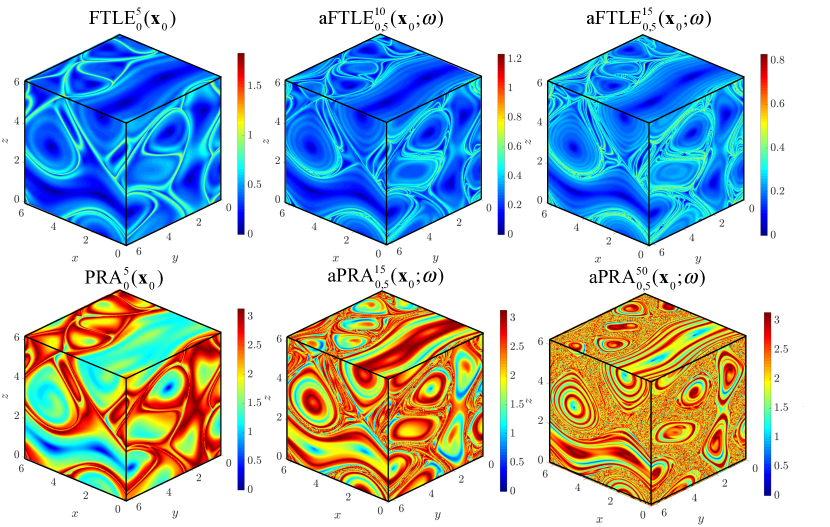
Figure 5: Passive and vorticity-based active versions of the FTLE and PRA diagnostics for the unsteady ABC flow (70), computed over the same time interval ($[t_{0},t_{1}]=[0,5]$) and with the same spatial resolution ($300^{3}$ grid points in the spatial domain $[0,2\pi]^{3}$). Two values for the barrier-time $s$ were selected to illustrate the increasing spatial resolution and convergence of hyperbolic barriers by the aFTLE and of elliptic barriers by the aPRA under increasing $s$-times. With the exception of the passive PRA, all diagnostics shown here are objective.

The $t_{1}=t_{0}\equiv t$ limit of the aFTLE field in eq. (82) is

$$\mathrm{aFTLE}_{t,t}^{s}(\mathbf{x};\mathbf{f})=\frac{1}{2s}\log\lambda_{\mathrm{max}}\left(\bm{\mathcal{C}}_{t,t}^{s}\left(\mathbf{x}\right)\right).$$ (83)

Here $\bm{\mathcal{C}}_{t,t}^{s}\left(\mathbf{x}\right)$ is simply computed from the autonomous flow map $\bm{\mathcal{F}}_{t,t}^{s}(\mathbf{x})$ of the instantaneous barrier equation (22), with the instantaneous time $t$ playing the role of a constant parameter in the computation. Again, the time-like evolutionary variable $s$ in this computation can be arbitrarily large in norm, as long as the trajectories generated by the barrier flow map $\bm{\mathcal{F}}_{t,t}^{s}(\mathbf{x})$ stay in the domain $U$ over which the barrier vector field $\mathbf{b}_{t}^{t}(\mathbf{x})$ is known. This guarantees convergence and higher resolution in the detection of instantaneous objective barriers from $\mathrm{aFTLE}_{t,t}^{s}(\mathbf{x};\mathbf{f})$ when compared with $\mathrm{FTLE}_{t}^{t}(\mathbf{x})$. The only practical limitation to resolving the details of active barriers via aFTLE is the spatial resolution of the available data.

8.5 Passive PRA vs. active PRA (aPRA)

By the polar decomposition theorem (Gurtin, Fried & Anand 2013), the deformation gradient $\bm{\nabla}\mathbf{F}_{t_{0}}^{t_{1}}(\mathbf{x}_{0})$ can be uniquely decomposed as

$$\bm{\nabla}\mathbf{F}_{t_{0}}^{t_{1}}=\mathbf{R}_{t_{0}}^{t_{1}}\mathbf{U}_{t_{0}}^{t_{1}},$$ (84)

with the proper orthogonal rotation tensor $\mathbf{R}_{t_{0}}^{t_{1}},$ the symmetric and the positive definite right stretch tensor $\mathbf{U}_{t_{0}}^{t_{1}}$ . The decomposition (84) means that a general deformation can locally always be viewed as triaxial stretching and compression followed by a rigid-body rotation. One can verify by direct substitution into (84) that $\mathbf{R}_{t_{0}}^{t_{1}}$ and $\mathbf{U}_{t_{0}}^{t_{1}}$ must be of the form

$$\mathbf{U}_{t_{0}}^{t_{1}}=\left[\mathbf{C}_{t_{0}}^{t_{1}}\right]^{1/2},\qquad\mathbf{R}_{t_{0}}^{t_{1}}=\bm{\nabla}\mathbf{F}_{t_{0}}^{t_{1}}\left[\mathbf{U}_{t_{0}}^{t_{1}}\right]^{-1},$$ (85)

with $\mathbf{C}_{t_{0}}^{t}$ defined in (78). The first equation in (85) shows that $\mathbf{U}_{t_{0}}^{t}$ can be computed using the singular-value-decomposition of $\mathbf{C}_{t_{0}}^{t}$. With $\mathbf{U}_{t_{0}}^{t_{1}}$ at hand, one can compute the rotation tensor $\mathbf{R}_{t_{0}}^{t_{1}}$ from the second equation of (85).

Farazmand & Haller (2016) show that $\mathbf{R}_{t_{0}}^{t_{1}}(\mathbf{x}_{0})$ rotates material elements around an axis of rotation by the polar rotation angle (PRA) satisfying

$$\mathrm{PRA}_{t_{0}}^{t_{1}}(\mathbf{x}_{0})=\cos^{-1}\left[\frac{1}{2}\left(\mathrm{{tr}\,}\mathbf{R}_{t_{0}}^{t_{1}}(\mathbf{x}_{0})-1\right)\right]=\cos^{-1}\left[\frac{1}{2}\left(\sum_{i=1}^{3}\left\langle\bm{\xi}_{i}(\mathbf{x}_{0}),\bm{\eta}_{i}(\mathbf{x}_{0})\right\rangle-1\right)\right],$$ (86)

with $\bm{\xi}_{i}(\mathbf{x}_{0})$ and $\bm{\eta}_{i}(\mathbf{x}_{0})$ denoting the right and left singular vectors of $\bm{\nabla}\mathbf{F}_{t_{0}}^{t}(\mathbf{x}_{0})$. For 2D flows viewed as 3D flows with a symmetry, the intermediate eigenvalue of $\mathbf{C}_{t_{0}}^{t}$ is always one, which simplifies $\mathrm{PRA}_{t_{0}}^{t_{1}}(\mathbf{x}_{0})$ to

$$\mathrm{PRA}_{t_{0}}^{t_{1}}(\mathbf{x}_{0})=\cos^{-1}\left\langle\bm{\xi}_{1}(\mathbf{x}_{0}),\bm{\eta}_{1}(\mathbf{x}_{0})\right\rangle=\cos^{-1}\left\langle\bm{\xi}_{2}(\mathbf{x}_{0}),\bm{\eta}_{2}(\mathbf{x}_{0})\right\rangle,\quad\mathbf{x}_{0}\in\mathbb{R}^{2}.$$ (87)

Farazmand & Haller (2016) propose $\mathrm{PRA}_{t_{0}}^{t_{1}}(\mathbf{x}_{0})$ as a diagnostic tool for elliptic (rotational) LCS. They find that nested circular or toroidal level sets of $\mathrm{PRA}_{t_{0}}^{t_{1}}(\mathbf{x}_{0})$ indeed highlight elliptic LCS significantly sharper than FTLE valleys do. They also show, however, that these level sets are only objective for 2D flows. Similarly to FTLE calculations for $\mathbf{u}(\mathbf{x},t)$, the spatial scales resolved by the passive PRA in 2D flows are limited by the length of the time interval $[t_{0},t_{1}].$ For 3D flows, an additional limitation of the PRA is the non-objectivity of its level surfaces. The instantaneous limit $t_{0}=t_{1}\equiv t$ of the PRA gives $\mathrm{PRA}_{t}^{t}(\mathbf{x})\equiv 0$, and hence this diagnostic is unable to detect instantaneous limits of elliptic OECS.

In contrast, using the active rotation tensor

$$\bm{\mathcal{R}}_{t_{0,}t_{1}}^{s}=\bm{\nabla}\bm{\mathcal{F}}_{t_{0},t_{1}}^{s}\left[\bm{\mathcal{C}}_{t_{0},t_{1}}^{s}\right]^{-1/2},$$ (88)

the corresponding active PRA (aPRA) is obtained in 3D as

$$\mathrm{aPRA}_{t_{0,}t_{1}}^{s}(\mathbf{x}_{0};\mathbf{f})=\cos^{-1}\left[\frac{1}{2}\left(\mathrm{{tr}\,}\bm{\mathcal{R}}_{t_{0,}t_{1}}^{s}(\mathbf{x}_{0})-1\right)\right]=\cos^{-1}\left[\frac{1}{2}\left(\sum_{i=1}^{3}\left\langle\bm{\xi}_{i}^{a}(\mathbf{x}_{0}),\bm{\eta}_{i}^{a}(\mathbf{x}_{0})\right\rangle-1\right)\right],$$ (89)

with $\bm{\xi}_{i}^{a}(\mathbf{x}_{0})$ and $\bm{\eta}_{i}^{a}(\mathbf{x}_{0})$ denoting the right and left singular vectors of the active deformation gradient $\bm{\nabla}\bm{\mathcal{F}}_{t_{0},t_{1}}^{s}$. For 2D flows, the corresponding formula is

$$\mathrm{aPRA}_{t_{0,}t_{1}}^{s}(\mathbf{x}_{0};\mathbf{f})=\cos^{-1}\left\langle\bm{\xi}_{1}^{a}(\mathbf{x}_{0}),\bm{\eta}_{1}^{a}(\mathbf{x}_{0})\right\rangle=\cos^{-1}\left\langle\bm{\xi}_{2}^{a}(\mathbf{x}_{0}),\bm{\eta}_{2}^{a}(\mathbf{x}_{0})\right\rangle,\quad\mathbf{x}_{0}\in\mathbb{R}^{2}.$$ (90)

Unlike for the passive PRA defined in (86), the spatial scales resolved by the aPRA can be gradually refined by increasing the time-like parameter $s$ in $\mathrm{aPRA}_{t_{0,}t_{1}}^{s}$. As in the case of the aFTLE, this increase is possible as long as the underlying trajectories $\tilde{\mathbf{x}}_{0}\left(s;0,\mathbf{x}_{0}\right)$ of the barrier equation for $\mathbf{f}$ stay in the spatial domain $U$ where $\mathbf{u}(\mathbf{x},t)$ is known. As for aFTLE, the spatial resolution of the active barriers discoverable by aPRA is only limited by the resolution of the available velocity data. Figure 5 illustrates the substantial refinement and convergence for increasing $s$-values obtained from aPRA relative to the passive PRA computed over the same time interval $[t_{0},t_{1}]=[0,5]$ for the unsteady ABC flow (70).

Another major advantage of $\mathrm{aPRA}_{t_{0,}t_{1}}^{s}$ over $\mathrm{PRA}_{t_{0}}^{t_{1}}$ is the objectivity of $\mathrm{aPRA}_{t_{0,}t_{1}}^{s}$, which follows from the objectivity of the barrier vector field $\mathbf{b}_{t_{0}}^{t_{1}}(\mathbf{x}_{0})$. Additionally, structures revealed by $\mathrm{aPRA}_{t_{0,}t_{1}}^{s}$ always converge as $s$ is increased, because $\mathrm{aPRA}_{t_{0,}t_{1}}^{s}$ operates on a steady flow, even though $\mathbf{u}(\mathbf{x},t)$ is unsteady. Finally, unlike $\mathrm{PRA}_{t_{0}}^{t_{1}}(\mathbf{x}_{0})$, its active version, $\mathrm{aPRA}_{t_{0,}t_{1}}^{s}$, has a non-degenerate instantaneous limit, $\mathrm{aPRA}_{t_{,}t}^{s}(\mathbf{x};\mathbf{f})$, which is just the PRA computed for the Eulerian barrier equation (22) over the barrier-time interval $[0,s]$. This limit enables the detection of instantaneous limits of active elliptic LCSs as active elliptic OECSs.

8.6 Relationship between active and passive LCS diagnostics

Active LCS diagnostics are applied to barrier vector fields, whereas passive LCS diagnostics are applied to the underlying velocity field. As a consequence, active barriers highlighted by active LCS methods generally differ from passive barriers (coherent structures) detected by passive LCS methods. This is no surprise, given that these two types of barriers are constructed from different principles.

As an extreme case, all Eulerian and Lagrangian active barriers coincide with their passive counterparts in directionally steady Beltrami flows (see section 7.2). Therefore, the closer a generic flow is to a Beltrami flow in a given region, the closer its active and passive barriers will be to each other in that region. More broadly, the more correlated the velocity field is with its Laplacian (i.e., with the diffusive force field), the closer the Lagrangian and Eulerian momentum barriers are expected to be to their passive counterparts. Similarly, the more correlated the velocity field is with the vorticity Laplacian (i.e., with the curl of the diffusive force field), the closer the Lagrangian and Eulerian vorticity barriers will be to their passive counterparts.

As another extreme case, inviscid flows have barrier equations with identically vanishing right-hand sides. This is because there is no viscous transport in such flows and hence active barriers are not well-defined. As a consequence, aFTLE and aPRA will identically vanish for such flows, while passive FTLE and PRA will only vanish if the inviscid flow has a spatially independent velocity field. Therefore, the more inviscid the flow is in a region, the more its active and passive barriers will differ from each other in that region.

A notable case between Beltrami and inviscid flows is a Lamb–Oseen velocity field modeling a vortex decaying due to viscosity (Saffman et al. 1992). Along each cylindrical streamsurface surrounding the origin in this flow, the viscous force is a constant negative multiple of the velocity at any given time. This immediately implies that all Eulerian active and passive barriers to momentum transport coincide with the cylindrical streamsurfaces of Lamb–Oseen vortices, even though their velocity field is not Beltrami. Indeed, we do find in our upcoming 2D and 3D turbulence examples that strong enough vortices have very similar overall signatures in the active and the passive LCS diagnostic fields, with the former field providing more detail. This stands in contrast to hyperbolic mixing regions outside those vortices, in which active and passive LCS diagnostics may differ substantially.

9 Active barriers in specific unsteady flows

In this section, we illustrate the numerical implementation of our results and the use of active LCS diagnostics (see section 8) on 2D homogeneous, isotropic turbulence and a 3D turbulent channel flow. The scripts we have used to compute active barriers in these examples can be downloaded from https://github.com/LCSETH?tab=repositories.

9.1 Two-dimensional homogeneous, isotropic turbulence

Here we evaluate our 2D results from section 7.1 on active barriers in a 2D turbulence simulation over a spatially periodic domain $U=[0,2\pi]\times[0,2\pi]$. Since all computations will be two-dimensional in this section, we drop the hat from the notation we used in section 7.1 for 2D variables.

Obtained from a pseudo-spectral code applied to the 2D, incompressible Navier-Stokes equation (see Farazmand, Kevlahan & Protas 2011), the spatial coordinates are resolved using $1024^{2}$ Fourier modes with $2/3$ dealiasing. The viscosity is $\nu=2\times 10^{-5}$. This data set comprises $251$ equally spaced velocity field snapshots spanning the time interval $[0,50]$. Whenever a numerical integration scheme is required, i.e., advection of particles and integration of the barrier fields, the Runge-Kutta 4 algorithm is employed. The same data set was already analyzed by Katsanoulis et al. (2019), who located vortex boundaries as barriers to the diffusive transport of vorticity using the theory of constrained diffusion barriers from Haller, Karrasch & Kogelbauer (2019). In contrast, here we use appropriate 2D, steady barrier equations (47)-(48) and (50)-(51) (see also Remark 8) to visualize Lagrangian and objective Eulerian coherent vortices as regions bounded by maximal barriers to active transport.

9.1.1 Eulerian active barriers

For the instantaneous barrier calculations, we use the first snapshot of the dataset at time $t=0$ and we compute the right-hand side of eqs. (48) and (51) using a grid of $1024\times 1024$ points. In our experience, this grid spacing is much smaller than the size of the coherent vortices in this flow. As a consequence, the results do not change appreciably under further grid refinements, as long as one targets structurally stable objects in the Lagrangian particle dynamics, as we do (see Definition 2). For vorticity barriers, we use the 2D version of eq. (77) to illustrate the computational procedure for barriers in lower-resolved data. We then proceed to compute the aFTLE and aPRA for both the momentum and vorticity barrier fields from eqs. (83) and (90) using a central finite-differencing scheme for the active flow map gradient required in eq. (81).

We focus on the region $\left[2.8,4.9\right]\times\left[1,3\right]$ of the full computational domain to illustrate the level of spatial detail we obtain from instantaneous velocity data (see fig. 6). We note the striking differences in the quality of the delineated structures between the instantaneous limit of the passive FTLE and the momentum-based aFTLE of figure 6. Advective LCSs tend to have relatively weak signatures in the instantaneous limit of the FTLE field (see formula (80)) which is given by the dominant rate-of-strain eigenvalue field. In contrast, active barriers remain sharply defined in the aFTLE fields, which offer increasing refinement of the flow features under increasing $s$-times. The only limitation to this refinement is the resolution of the available data. This is apparent in the vorticity-based aFTLE in figure 6c, where the improvement is more modest, given that higher-order spatial derivatives need to be computed from the same data set.

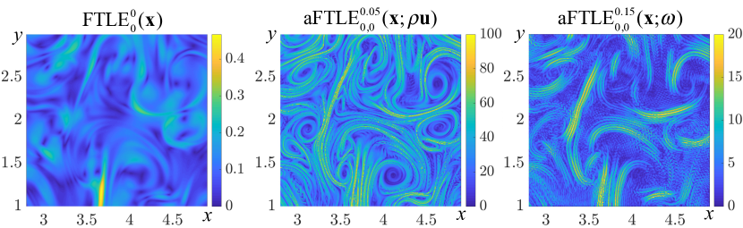
Figure 6: Comparison of the $t=0$ instantaneous limits of the passive FTLE, the aFTLE with respect to $\rho\mathbf{u}$ with $s=0.05$ and the aFTLE with respect to $\bm{\mathbf{\omega}}$ with $s=0.15$ in our 2D turbulence example.

Figure 7 focuses on momentum-based active barriers in one of the vortical regions revealed by figure 6. The aFTLE provides a clear demarcation of the main vortex, which becomes even more pronounced for longer $s$-times, revealing secondary vortices around its neighborhood. In contrast, none of these vortices are present in the passive FTLE in figure 7. A similar result emerges when the same region is analyzed using the aPRA field in the same figure. Specifically, the effect of progressive refinement with increasing $s$-times is more prominent here as a number of elliptic structures become visible in the main vortical region. In contrast, the instantaneous limit of the passive PRA returns identically zero values, as the instantaneous limit of all polar rotation angles is zero by definition.

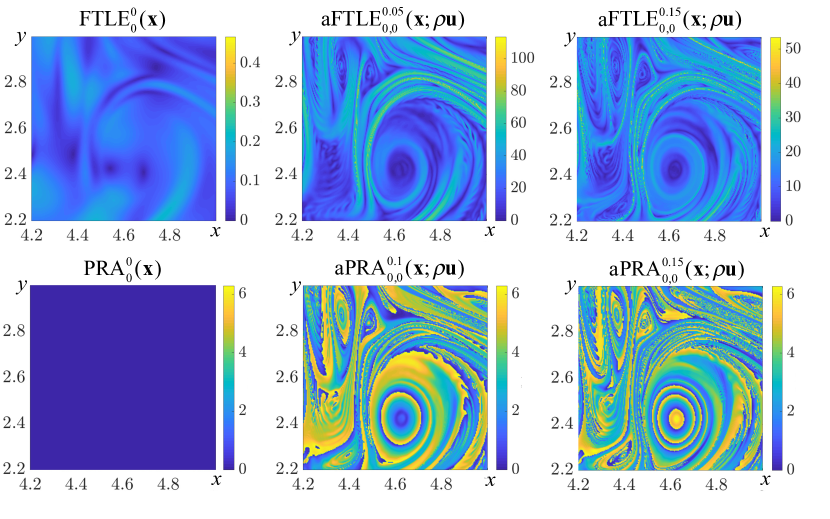
Figure 7: Comparison between the instantaneous limit of the passive FTLE (PRA) and the instantaneous limit of the momentum-based aFTLE (PRA) fields for $s=0.05$ and for $s=0.15$ in one of the vortical regions of our 2D turbulence example at $t=0$.

9.1.2 Lagrangian active barriers

For the Lagrangian computations in this example, we use the same, slightly oversampled grid of Katsanoulis et al. (2019) with $1100\times 1100$ equally spaced initial conditions and we advect them over the time interval $[0,25]$ using all the available velocity snapshots. To compute the required Lagrangian averages along trajectories, we use $25$ snapshots of the appropriate quantities as using more snapshots does not bring any noticeable changes to the resulting barrier fields. Based on that, we compute the expressions for the active barrier fields from eqs. (47) and (50), which we then use for the evaluation of the aFTLE and aPRA.

Comparisons between these scalar diagnostic fields and the passive FTLE and PRA are shown in figure 8. We observe that the momentum-based aFTLE and aPRA reveal structures inside the vortical regions in much finer detail, as they do not rely on substantial fluid particle separation. In agreement with our arguments in section 8.6, aFTLE and aPRA consistently refine the same coherent vortices indicated by FTLE and PRA. In the mixing regions surrounding those vortices, however, active and passive LCS diagnostics tend to identify different barriers. As in the case of our Eulerian barrier calculations in section 9.1.1, the vorticity-based aFTLE and aPRA provide a more moderate enhancement, because they rely on second derivatives of the velocity data.

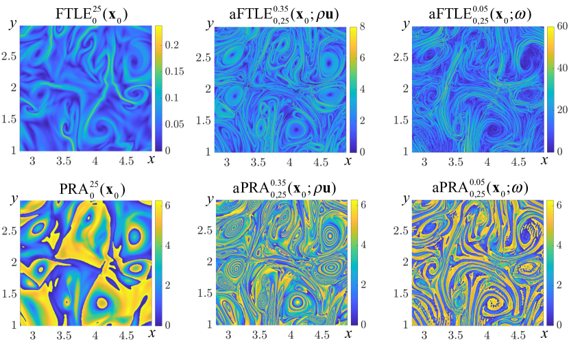
Figure 8: Comparison between the passive FTLE (PRA) and the momentum- and vorticity-based aFTLE (aPRA). All computations were performed over the time interval $[t_{0},t_{1}]=[0,25]$ on the domain $\left[2.8,4.9\right]\times\left[1,3\right]$.

Next, we illustrate the extraction of active barriers to the transport of momentum and vorticity as parametric curves. This is possible in 2D incompressible flows because the active barrier equations are Hamiltonian, and hence the barriers are level curves of a scalar function (see Theorems 6 and 7, as well as Remark 8). To perform this extraction, we follow the method presented in Haller et al. (2016) for the extraction of coherent Lagrangian vortex boundaries as outermost level sets of the Lagrangian-averaged vorticity deviation (LAVD). We will use the notation $H_{t_{0}}^{t_{1}}(\mathbf{x}_{0})$ to denote the relevant Hamiltonian from section 7.1. The algorithm is the same for all those Hamiltonians, but we will restrict our computations here to the Hamiltonian governing Lagrangian momentum-barriers in 2D, given by $H_{t_{0}}^{t_{1}}(\mathbf{x}_{0})=\nu\rho\,\overline{\omega\left(\mathbf{F}_{t_{0}}^{t}\left(\mathbf{x}_{0}\right),t\right)}$ (see eq. (47)).

In all our computations, we will focus on finding almost convex structurally stable level sets of $H_{t_{0}}^{t_{1}}(\mathbf{x}_{0})$ that encircle a single local maximum of $\left|H_{t_{0}}^{t_{1}}(\mathbf{x}_{0})\right|$. The need for relaxation of the strict convexity requirement in discrete data sets is discussed extensively in Haller et al. (2016), so we will skip it here. Along these lines, we introduce the convexity deficiency of a closed curve in the plane as the ratio of the area between the curve and its convex hull to the area enclosed by the curve, which we denote with $d_{max}$. The maximum $d_{max}$ we used for the different extracted barriers was $5\times 10^{-2}$.

Small-scale local maxima of $\left|H_{t_{0}}^{t_{1}}(\mathbf{x}_{0})\right|$ may appear either due to non-accurate resolution of these scales or because of computational noise. To address this issue, we only considered boundaries with arclength larger than a threshold $l_{min}$. This threshold was set to $0.4$ for all our computations because below this limit, boundaries contain too few grid points to be considered well-resolved.

The main steps of the extraction procedure are delineated in Algorithm 1. All the MATLAB codes used for the extraction of the barriers of this section can be found in the on-line supplementary materials.

Algorithm 1 Coherent Lagrangian and Eulerian vortex boundaries for two-dimensional flows

Input: A time-resolved two-dimensional velocity field (or a snapshot thereof in the Eulerian case).

1. For a grid of initial conditions $\mathbf{x}_{0}$, compute the $H_{t_{0}}^{t_{1}}(\mathbf{x}_{0})$.

2. Find local maxima of $\left|H_{t_{0}}^{t_{1}}(\mathbf{x}_{0})\right|$.

3. Detect initial vortex boundaries as outermost closed contours of $H_{t_{0}}^{t_{1}}(\mathbf{x}_{0})$ satisfying the following:

   1. The boundary encircles a local maximum of $\left|H_{t_{0}}^{t_{1}}(\mathbf{x}_{0})\right|$.

   2. The boundary has convexity deficiency less than a bound $d_{max}$.

   3. The boundary has arclength exceeding a threshold $l_{min}$.

Output: Initial positions of coherent Lagrangian or Eulerian vortex boundaries.

We apply this algorithm to extract an active material barrier to the transport of momentum with high precision as a parametrized curve. This closed active barrier is shown in red in figure 9. We also show the impact of this barrier on the momentum landscape in Eulerian and Lagrangian coordinates, respectively, for the initial and final times in $\left[0,25\right]$. Furthermore, for reference, we show an elliptic LCS (black) extracted as a closed level curve of the passive PRA through a selected point of the active barrier. As expected from our discussion in section 8.6, these active and passive elliptic barriers are very close to each other at the initial time and remain equally close during their material evolution. In the Eulerian frame, we observe that the extracted active and passive barriers shows no sign of filamentation throughout their whole extraction time. This is in agreement with the general expectation we stated earlier for diffusion-minimizing material curves. Furthermore, when viewed in the Lagrangian frame, we note the organizing role of the extracted barrier in the momentum landscape. Indeed, the barrier keeps encapsulating small values of the momentum norm for the entire extraction time.

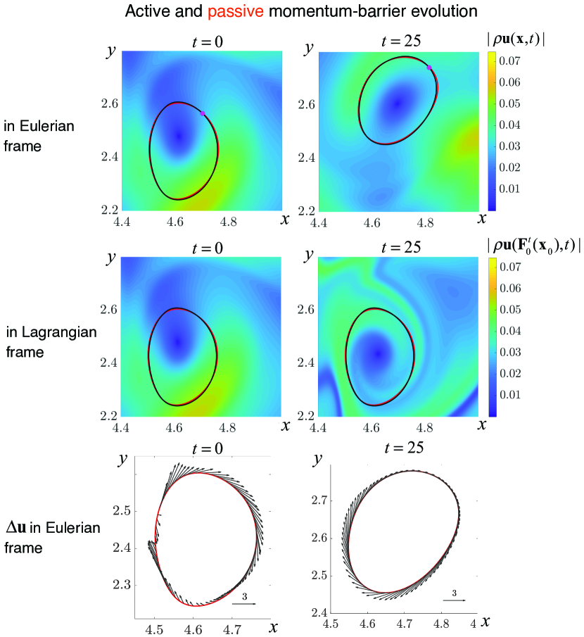
Figure 9: Evolution of an extracted active material barrier (red) to the diffusive transport of momentum in the Eulerian and the Lagrangian frame, superimposed on the distribution of the norm of the linear momentum. This barrier was identified as a level curve of the Hamiltonian $H_{t_{0}}^{t_{1}}(\mathbf{x}_{0})=\nu\rho\,\overline{\omega\left(\mathbf{F}_{t_{0}}^{t}\left(\mathbf{x}_{0}\right),t\right)}$. Black curve indicates an elliptic LCS extracted as a level curve of the passive PRA, launched from the highlighted point of the active barrier. Also shown are the instantaneous viscous forces (normalized by $\rho\nu$) acting on the evolving barrier.

Figure 9 also shows the instantaneous viscous force (normalized by $\rho\nu$) along the extracted active momentum barrier. Note that this force remains almost tangent to the barrier for the most part. There are, however, some notable exceptions, illustrating that these barriers are not constructed to be tangent to the viscous forces at every time instance. Rather, the viscous forces are tangent to the barriers in a time-averaged sense after being pulled back under the flow map to the initial configuration.

9.2 Three-dimensional turbulent channel flow

We consider now the 3D incompressible, turbulent flow of a Newtonian fluid in a doubly periodic channel, a well-studied physical setting for 3D coherent structure studies.

Our analysis relies on velocity snapshots from a mixed-discretization parallel solver of the incompressible Navier–Stokes equations in the wall-normal velocity and vorticity formulation, developed by Luchini & Quadrio (2006). The equations of motions are discretized via a Fourier–Galerkin approach along the two statistically homogeneous streamwise $\left(x\right)$ and spanwise $\left(z\right)$ directions. Fourth-order compact finite differences (Lele 1992) based on a five-point computational stencil are adopted in the wall-normal direction $\left(y\right)$.

The governing equations are integrated forward in time at constant power input (Hasegawa et al. 2014) with a partially-implicit approach, combining the three-step, low-storage Runge–Kutta (RK3) scheme with the implicit Crank–Nicolson scheme for the viscous terms. The friction Reynolds number is $Re_{\tau}=u_{\tau}h/\nu=200$, based on the friction velocity $u_{\tau}$, the channel half height $h$ and the kinematic viscosity $\nu$, which corresponds to a bulk Reynolds number $Re_{b}=U_{b}h/\nu=3177$, where $U_{b}$ is the bulk velocity. The computational domain is $L_{x}=4\pi h$ long and $L_{z}=2\pi h$ wide. The number of Fourier modes is 256 both in the streamwise and spanwise direction; the number of points in the wall-normal direction is 256, unevenly spaced in order to decrease the grid size near the walls. The corresponding spatial resolution in the homogeneous directions is $\Delta x^{+}=9.8$ and $\Delta z^{+}=4.9$ (without accounting for the additional modes required for dealiasing according to the 3/2 rule); the wall-normal resolution increases from $\Delta y^{+}=0.4$ near the walls to $\Delta y^{+}=2.6$ at the centreline, while the temporal resolution is kept constant at $\Delta t=0.005h/U_{b}$, corresponding to $\Delta t^{+}=0.063$. The superscript $+$ denotes nondimensionalization in viscous units, i.e. with $u_{\tau}$ and $\nu$. At each DNS timestep and thus with the same temporal resolution, a three-dimensional flow snapshot is stored for a total of 1500 snapshots. The 750^th snapshot in the series is stored at time $t=0$. This is the instant at which we compute the Eulerian barriers to active transport. The last 750 snapshots are utilised for the computation of the active barriers and passive forward FTLE, while the first 750 ones are used for calculating the passive backward FTLE. The integration time for the Lagrangian calculations has been chosen based on pair-dispersion statistics of Lagrangian tracers (see, for instance, Pitton et al. 2012). The averaging time for the bulk flow statistics is 8100 $U_{b}/h$. In the following, all quantities are nondimensionalized using $U_{b}$ and $h$ unless stated otherwise.

The active barriers are computed in a two-step procedure. First, the active barrier field $\mathbf{b}_{t_{0}}^{t_{1}}\left(\mathbf{x}_{0}\right)$, appearing at the right-hand side of the barrier equation (21), is computed. Then, the barrier ODE is solved and visualised via the FTLE and PRA diagnostics.

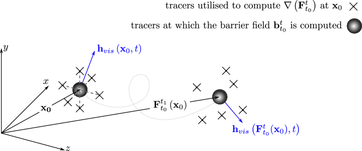
Figure 10: Sketch of the computational molecule utilised for the computation of the active barrier field $\mathbf{b}_{t_{0}}^{t_{1}}$. The large circle denotes the Lagrangian tracer at the center of the molecule, where the vector field $\mathbf{h}_{vis}$ is computed. The cross denotes the further six tracers utilised to compute $\nabla\mathbf{F}_{t_{0}}^{t_{1}}$.

For Eulerian barriers, the barrier vector field appearing in the instantaneous (or Eulerian) barrier equation (22) is readily computed from the velocity field data as $\mathbf{b}_{t}^{t}=\mathbf{h}_{vis}$. Differentiation of the velocity field is performed with the same discrete operators used during DNS. For material barriers, $\mathbf{b}_{t_{0}}^{t_{1}}\left(\mathbf{x}_{0}\right)$ is simply obtained as the temporal average of $\left(\mathbf{F}_{t_{0}}^{t_{1}}\right)^{\ast}\mathbf{h}_{vis}$, because $\det\nabla\mathbf{F}_{t_{0}}^{t_{1}}\left(\mathbf{x}_{0}\right)\equiv 1$ by incompressibility. In this case, the vector field $\mathbf{b}_{t_{0}}^{t_{1}}\left(\mathbf{x}_{0}\right)$ is discretised on a Cartesian grid similar to the one used for the velocity field; the only difference is that the number of collocation points along the $x$- and $z$-directions is increased to 384 via Fourier interpolation.

At time $t_{0}$, a set of tracers is seeded in the neighbourhood of each point $\mathbf{x}_{0}$ at which $\mathbf{b}_{t_{0}}^{t_{1}}\left(\mathbf{x}_{0}\right)$ needs to be computed. Each set (see figure 10) is composed by 7 tracers. The central tracer is exactly located at $\mathbf{x}_{0}$ and is the only one along which the vector field $\mathbf{h}_{vis}$ is also computed. The other tracers are shifted by $\epsilon_{i}$ along the positive and negative $i$th spatial direction and are utilised to compute $\nabla\mathbf{F}_{t_{0}}^{t_{1}}\left(\mathbf{x}_{0}\right)$ with second-order central finite differences. The shift $\epsilon_{i}$ is defined as $1/100$ of the minimum grid spacing along the $i$th spatial direction. A total of $2.64\times 10^{8}$ particles are seeded into the flow. The evolving positions of these tracers, which are images of their initial positions under the flow map $\mathbf{F}_{t_{0}}^{t_{1}}$, are advanced in time by integrating the $\mathbf{u}$ field with a third-order, four-stage Runge–Kutta algorithm. The vector fields $\mathbf{u}$ and $\mathbf{h}_{vis}$ required at the intermediate stages are obtained via linear interpolation of two consecutive flow snapshots and are evaluated at the particle position through a sixth-order, three-dimensional Lagrangian interpolation (van Hinsberg et al. 2012, Pitton et al. 2012) of the underlying vector field, which reduces to fourth-order only between the wall and the first grid point above it.

Once the (Lagrangian or Eulerian) barrier equation is available, its active flow map $\bm{\mathcal{F}}_{t_{0},t_{1}}^{s}$ is computed by solving the steady barrier ODE up to $s_{\mathrm{max}}=31.0$ and $s_{\mathrm{max}}=0.62$ for the momentum and vorticity barriers, respectively. We have chosen these $s$-times large enough for the computed barrier trajectories to reveal enough detail in the underlying barrier vector field but small enough to avoid accumulation of the integration error. The effect of changing the parameter $s_{\mathrm{max}}$ is shown in the additional material Movie 1.mp4 and Movie 2.mp4 for Eulerian momentum and vorticity barriers, respectively. The seeds for the flow map are arranged in a Cartesian grid identical to the one of the active barrier field for 3D computations of aFTLE/aPRA diagnostics, while the spatial resolution is increased by a factor 6 when only two-dimensional slices are computed. The comparison between the two resolutions has been utilised to verify the grid-independence of the results. The aFTLE and aPRA diagnostics are then computed according to equations (82) and (89), respectively.

9.2.1 Eulerian active barriers

Instantaneous aFTLE and aPRA are presented for $t=0$ in figures 11 and 12, respectively, and compared against their passive variants. Even though the results are computed for the complete three-dimensional field, only two-dimensional cross sections are presented in the following. In figures 11 and 12, a $\left(y-z\right)$ cross-section located at $x=2\pi h$ is shown. The 3D visualisation of the FTLE and PRA fields poses challenges in its own, which are subjects of ongoing research in computer visualisation (see, e.g., Sadlo & Peikert 2009, Schindler et al. 2012) and are outside the scope of the present study. The 2D visualization in different cross sections results in different local flow structures which are, nevertheless, all reminiscent of classically known structures in channel flows. These include low-speed streaks, quasi-streamwise and hairpin vortices and packets thereof (Robinson 1991). The supplementary materials Movie 3.mp4 and Movie 4.mp4 show how figure 11(b-c) change throughout the channel length.

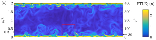
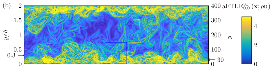
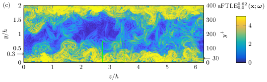
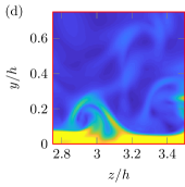
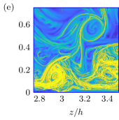
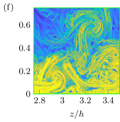
Figure 11: Comparison between the instantaneous limit of (a,d) the passive FTLE, (b,e) the aFTLE with respect to $\rho\mathbf{u}$ and (c,f) the aFTLE with respect to $\bm{\omega}$ at $t=0$ in a cross-sectional plane at $x/h=2\pi$. The panels (d-f) magnify the region denoted with a rectangle in panels (a-c). All computations in the figure were performed on the same snapshot of the velocity field at $t=0$.

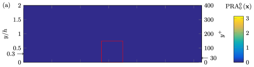
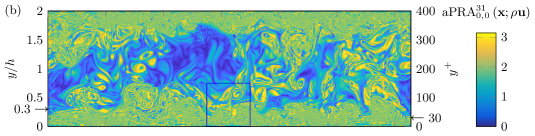
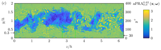
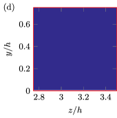
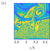
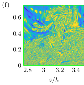
Figure 12: Comparison between the instantaneous limit of (a,d) the passive PRA (which is identically zero), (b,e) the aPRA with respect to $\rho\mathbf{u}$ and (c,f) the aPRA with respect to $\bm{\omega}$ at $t=0$ in a cross-sectional plane at $x/h=2\pi$. The panels (d-f) magnify the region denoted with a rectangle in panels (a-c). All computations in the figure were performed on the same snapshot of the velocity field at $t=0$.

As already seen for 2D turbulence in §9.1, the aFTLE and aPRA highlight a broader range of structures in more detail from the same velocity data when compared to their passive variants. (Recall that the instantaneous limit of the passive PRA, in fact, vanishes identically, and hence reveals no elliptic coherent structures from a single velocity snapshot.) The Eulerian active barriers revealed by aFTLE and aPRA appear in figures 11 and 12 as an abundance of intersections of 2D surfaces with the selected cross section. Limiting to visual inspection, we recognise several open (or hyperbolic) barriers as ridges of the aFTLE fields. Given the quasi-streamwise nature of turbulent structures in wall-bounded flows, vortical (or elliptic) barriers to transport are often observed in cross-sectional planes as aFTLE ridges wrapping around closed regions, which are also captured as level sets of the corresponding aPRA fields. Example of such regions are shown in the magnifications of panels (d-f) in figures 11 and 12.

The results also reveal that large prominent aFTLE ridges penetrate into and span the bulk flow region, sometimes connecting the channel halves, as visible in 11(b) between $3\leq z/h\leq 3.5$ and $0.3\leq y/h\leq 1.5$. Other regions, such as between $2\leq z/h\leq 3$ and $0.5\leq y/h\leq 1.5$ in the same figure, display practically no discernible barriers and are bounded by the envelopes of filamented open (hyperbolic) transport barriers, which are finite-time generalizations of infinite-time classic stable and unstable manifolds. Unlike in previous approaches, however, these finite-time invariant manifolds are constructed here as perfect material barriers to active transport, rather than as Lagrangian coherent structures acting as backbones of advected fluid-mass patterns (Haller 2015).

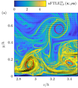
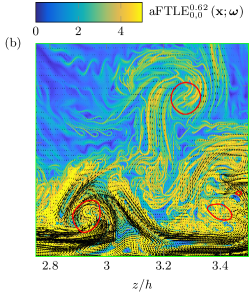
Figure 13: Eulerian active barriers of (a) $\rho\mathbf{u}$ and (b) $\bm{\omega}$ at $t=0$ in a cross-sectional plane located at $x/h=2\pi$. The colormap shows the respective aFTLE fields, the vectors show the cross-sectional components of the underlying active barrier field, while the red lines are level-set curves $\lambda_{2}^{+}(\mathbf{x},t)=-0.015$ of the Eulerian vortex identification criterion proposed by Jeong et al. (1997)

.

Figure 13 shows the Eulerian active barrier vector field of (a) $\rho\mathbf{u}$ and (b) $\bm{\omega}$ superimposed to the respective aFTLEs already shown in figure 11(e-f). Level-set curves of the $\lambda_{2}(\mathbf{x},t)=-0.015$ field (Jeong & Hussein 1995), a common visualization tool for coherent vortical structures in wall-bounded turbulence, are also shown. The scalar field $\lambda_{2}(\mathbf{x},t)$ is defined as the instantaneous intermediate eigenvalue of the tensor field $\mathbf{S}^{2}(\mathbf{x},t)+\mathbf{W}^{2}(\mathbf{x},t)$, with $\mathbf{S}$ and $\mathbf{W}$ defined in eq. (71). This choice follows the heuristic convention to select a $\lambda_{2}^{+}$ value slightly below the negative of the r.m.s. peak of $\lambda_{2}(\mathbf{x},t)$ across the channel (Jeong et al. 1997), which is approximately $0.0125$ in our case.

Compared to the passive material barriers shown in figure 11(d), we observe that the active barriers not only yield a remarkably more complex flow structure but also carry a completely different physical meaning. Since the active barriers minimise the diffusive transport of, in this case, linear momentum or vorticity, we find that the cross-sectional components of the active barrier vector field $\mathbf{b}_{t}^{t}$ are parallel to the aFTLE ridges. This indicates that the resultant force of the viscous stresses is tangential to Eulerian active barriers of momentum transport. As noted previously, momentum barriers in $\left(y-z\right)$ cross-sections can roll-up into spiral patterns or form closed surfaces. In regions where this occurs, figure 13(a) shows that closed level-set curves of $\lambda_{2}$, typically used as indicators for the presence of quasi-streamwise vortices, tend to be found. This suggests that boundaries of quasi-streamwise vortices act as Eulerian active barriers to the transport of linear momentum. Interestingly, we find that the circulation of the active momentum barrier field in such areas is of opposite sign than the one of the velocity field. This indicates that viscous forces oppose the vortical motion that is observed in the analyzed snapshots. In addition, Eulerian active barriers of vorticity tend to enter regions of closed momentum barriers or level-set curves of $\lambda_{2}$, thus highlighting regions in which vorticity diffuses into the vortex or is dissipated by viscosity.

Despite some similarities, it is important to note the practical and fundamental differences between the Eulerian momentum barriers and level-set surfaces of $\lambda_{2}$. On the fundamental side, we mention that the active barriers are objective, they have clear implications for the viscous transport of the active vector field and, most importantly, that they are extensible by definition to material barriers, thus accounting for the Lagrangian coherence of the barriers themselves. On the practical side, Eulerian active barriers do not require the convenient but arbitrary choice of a threshold and deliver information on the full active transport geometry, rather than just providing a few isolated curves.

9.2.2 Lagrangian active barriers

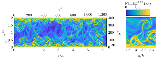
Figure 14: Passive backward $\mathrm{FTLE}_{0}^{-3.75}\left(\mathbf{x}_{0}\right)$ in a cross-sectional plane at $x/h=2\pi$. The right panel magnifies the region denoted with a rectangle in the left panel.

Figure 14 shows attracting material surfaces as passive backward $\mathrm{FTLE}_{0}^{-3.75}\left(\mathbf{x}_{0}\right)$ at the same $\left(y-z\right)$ cross-section located at $x=2\pi h$ discussed in §9.2.1. These attracting material surfaces, forming the cores of experimentally observed fluid trajectory patterns at time $t=0$, show a striking resemblance to the Eulerian active barriers to linear momentum indicated in figure 11(b,e) by the $\mathrm{aFTLE}_{0,0}^{31}\left(\mathbf{x}_{0},\rho\mathbf{u}\right)$ field. The close similarity between the two is not fully surprising. At the present low value of Reynolds number viscous effects dominate throughout a significant portion of the channel, and thus determine both the characteristics of the Eulerian momentum barriers and the finite-time dynamics of particle motion. The temporal horizon, over which the analogy between $\mathrm{FTLE}_{0}^{-3.75}\left(\mathbf{x}_{0}\right)$ and $\mathrm{aFTLE}_{0,0}^{31}\left(\mathbf{x}_{0},\rho\mathbf{u}\right)$ is observed, is expected to decrease with increasing Reynolds number, as the viscosity-dominated inner layer shrinks compared to the channel height. Whether the observed similarity holds at higher values of $Re$ is to be verified in later studies with high-$Re$ data. However, it is remarkable that the Eulerian momentum barriers, which are computed utilising a single flow snapshot, reproduce the same features of material surfaces obtained from a Lagrangian computation, which requires storing the temporal evolution of the flow.

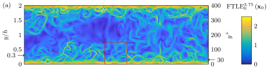
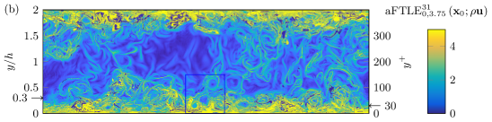
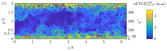
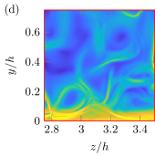
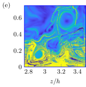
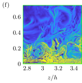
Figure 15: Comparison between (a,d) the passive FTLE, (b,e) the aFTLE with respect to $\rho\mathbf{u}$ and (c,f) the aFTLE with respect to $\bm{\omega}$ in a cross-sectional plane at $x/h=2\pi$. The integration interval is for all cases between $t_{0}=0$ and $t_{1}=3.75$. The panels (d-f) magnify the region denoted with a rectangle in panels (a-c).

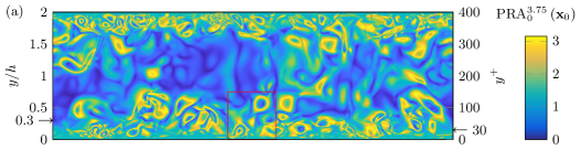
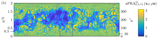
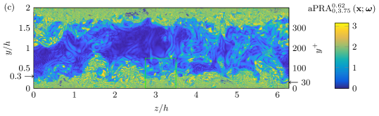
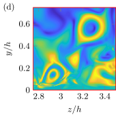
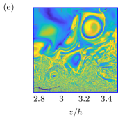
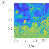
Figure 16: Comparison between (a,d) the passive PRA, (b,e) the aPRA with respect to $\rho\mathbf{u}$ and (c,f) the aPRA with respect to $\bm{\omega}$ in a cross-sectional plane at $x/h=2\pi$. The integration interval is for all cases between $t_{0}=0$ and $t_{1}=3.75$. The panels (d-f) magnify the region denoted with a rectangle in panels (a-c).

Figures 15 and 16 show aFTLE and aPRA computed for momentum- and vorticity-based material barriers in a $\left(y-z\right)$ cross-section located at $x=2\pi h$ and compare them against their passive variants. The integration interval is for all cases between $t_{0}=0$ and $t_{1}=3.75$ which corresponds to a time interval of 750 viscous units. The figures clearly show that some features of the Eulerian active barriers discussed in §9.2.1, such as the spiralling or closed patterns of $\mathrm{aFTLE}_{0,0}^{31}\left(\mathbf{x},\rho\mathbf{u}\right)$, do have a material character, since they persist almost unchanged over the temporal interval which we have considered. Examples are shown in the magnification of figures 15(e) and 16(e), showing promise for active LCS diagnostics in studying the lifetime of vortical structures in wall-bounded turbulence (Quadrio & Luchini 2003). In the vicinity of the wall, characterised by the strong intermittent turbulent events rapidly evolving with the viscous timescale, less detail is visible in the barriers, due to the lack of material coherence for the considered time frame. Consistent with the general principle discussed in section 8.6, passive and active LCS diagnostics tend to highlight the same vortical regions, but tend to differ in the mixing regions surrounding the vortices. As in our 2D turbulence example, while the vorticity-based aFTLE and aPRA plots show a major enhancement over passive FTLE and PRA, some of their details are less clearly defined in comparison to their momentum-based counterparts. Again, this is due to the additional spatial differentiation involved in computing active LCS diagnostics for the vorticity compared to the same computation for the linear momentum.

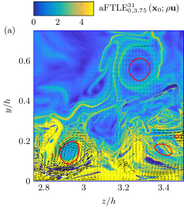
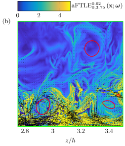
Figure 17: Material active barriers of (a) $\rho\mathbf{u}$ and (b) $\bm{\omega}$ at $t=0$ in a cross-sectional plane located at $x/h=2\pi$ and for an integration interval between $t_{0}=0$ and $t_{1}=3.75$. The colormap shows the respective aFTLE fields, the vectors show the cross-sectional components of the underlying active barrier field, while the red lines are level-set curves $\lambda_{2}^{+}(\mathbf{x},t)=-0.015$ of the Eulerian vortex identification criterion proposed by Jeong et al. (1997) at the instant $t_{0}=0$.

Figure 17 shows the material active barrier vector field of (a) $\rho\mathbf{u}$ and (b) $\bm{\omega}$ superimposed to the respective aFTLEs already shown in figure 15(e-f). Level-set curves of the $\lambda_{2}(\mathbf{x},t)=-0.015$ field at the temporal instant $t=t_{0}=0$ are also shown. It is confirmed that with the present definition of active barriers, the active vector field is tangent to the detected barriers visualised here as aFTLE ridges, in a temporally-averaged sense. Figure 17(a) shows that closed $\mathrm{aFTLE}_{t_{0},t_{1}}^{s}\left(\mathbf{x}_{0},\rho\mathbf{u}\right)$ ridges can be in some instances close to level-set curves of the $\lambda_{2}$ criterion, as for instance at $(y/h,z/h)\approx(0.15,2.9)$ and $(0.55,3.3)$. In this sense, the material momentum barriers can be utilised as means to objectively identify vortical structures which play a role in inhibiting momentum transport and preserve material coherence over the considered time frame, without resorting to arbitrary choices of level-sets of $\lambda_{2}$. In the present example, we find streamwise vortices that are bounded by active momentum barriers for a time period of 750 viscous units.

10 Conclusions

We have developed an approach to identify coherent structure boundaries as material surfaces that minimize the diffusive transport of active physical quantities intrinsic to the flow. We have also argued that instantaneous limits of these active Lagrangian transport barriers provide objective Eulerian barriers to the short-term redistribution of active vector fields.

Our analysis shows that in incompressible Navier–Stokes flows, active material barriers to transport evolve from structurally stable 2D stream-surfaces of an associated steady vector field, the barrier vector field $\mathbf{b}_{t_{0}}^{t_{1}}(\mathbf{x}_{0})$. This vector field is the time-averaged pull-back of the viscous terms in the evolution equation of the active vector field. For $t_{0}=t_{1}$, instantaneous limits of these material barriers to linear momentum are surfaces to which the viscous forces acting on the fluid are tangent. Similarly, instantaneous limits to active barriers to vorticity are surfaces tangent to the curl of viscous forces.

We have obtained that material and Eulerian active barriers in 3D unsteady Beltrami flows coincide exactly with invariant manifolds of the Lagrangian particle motion. This is noteworthy because all prior LCS methods applied to Beltrami flows would locate these barriers, at best, approximately for large enough extraction times, rather than exactly from arbitrary short extraction times, as the present approach does. The reason is that the present approach to material barriers does not rely on quantifying fluid particle separation or lack thereof, as purely advective LCS-approaches do. Instead, this approach seeks material surfaces that are most resistant to the diffusive transport of intrinsic physical quantities, such as momentum and vorticity. This dynamical extremum problem can be solved without the need for fluid particles to show large separation.

We have argued and numerically verified that, in comparison to their purely advective versions, active LCS reveal coherent vortices in much larger detail. Indeed, we have found the momentum-based aFTLE and the aPRA to outperform the purely advective FTLE and PRA significantly on vortices of the same finite-time velocity data set. In contrast, active and passive barriers are expected to differ significantly in mixing regions surrounding those vortices, as we have indeed found in our 2D and 3D turbulence examples. The refinement of vortical regions from vorticity-based aFTLE and aPRA is also tangible but more modest, as that computation involves one more spatial derivative and hence is more prone to numerical error. In addition, $\mathrm{aFTLE}_{t_{0},t_{1}}^{s}$ and $\mathrm{aPRA}_{t_{0},t_{1}}^{s}$ converge as the barrier-time $s$ increases, whereas $\mathrm{FTLE}_{t_{0}}^{t}$ and $\mathrm{PRA}_{t_{0}}^{t}$ generally do not converge in unsteady flows as the physical time $t$ increases. The convergence of $\mathrm{aFTLE}_{t_{0},t_{1}}^{s}$ and $\mathrm{aPRA}_{t_{0},t_{1}}^{s}$ enables a scale-dependent exploration of active barriers, with smaller spatial scales gradually revealed under increasing barrier times $s$.

A further advantage of the dynamically active approach to transport-barrier analysis is that an active Poincaré map (i.e., Poincaré map applied to the barrier equations $\mathbf{x}_{0}^{\prime}=\mathbf{b}_{t_{0}}^{t_{1}}(\mathbf{x}_{0})$) is a well-defined, time-independent map that can be iterated for visualization if barrier trajectories return to the Poincaré section. In contrast, no time-independent return map can be defined and iterated for the unsteady fluid-particle equation of motion $\dot{\mathbf{x}}=\mathbf{u}(\mathbf{x},t)$, because each subsequent return to a Poincaré section is governed by a different map.

The 2D versions of our results provide the simplest available objective LCS criteria, identifying barriers to active transport as level curves of appropriate Hamiltonians that are functions of the scalar vorticity. This follows from the fact that the 2D barrier equations turn out to be autonomous, planar Hamiltonian systems, and hence are, in principle, integrable. We have found, however, that active LCS diagnostics applied to these autonomous but highly complex planar Hamiltonian systems give a more robust and detailed localization of coherent vortex boundaries than level-curve identification of their numerically generated Hamiltonians.

Eulerian active barriers (identified from the steady dynamical system $\mathbf{x}^{\prime}=\mathbf{b}_{t}^{t}(\mathbf{x})$) provide an objective and parameter-free alternative to currently used, observer-dependent flow-visualization tools, such as level surfaces of the velocity norm, of the velocity components and of the $Q$-, $\Delta$- and $\lambda_{2}$-fields. Undoubtedly, the implementation of the latter tools is appealingly simple via automated level-surface visualization packages. Yet such evolving surfaces are observer-dependent and non-material, thereby lacking any experimental verifiability. In addition, beyond the simplicity of generating coherent structure boundaries as level sets of these scalar fields, the physical meaning of such level sets remains unclear.

The objectivity of the barrier vector field $\mathbf{b}_{t_{0}}^{t_{1}}$ implies that any Galilean-invariant vortex criterion mentioned in the Introduction becomes automatically objective when applied to $\mathbf{b}_{t_{0}}^{t_{1}}$, as opposed to the velocity field $\mathbf{u}$. This fact does not eliminate the heuristic nature of these criteria but at least makes the structures they return independent of the observer. The physical rationale for applying vortex- or LCS-criteria to the barrier vector field instead of the velocity field is that active barriers have a well-defined and readily quantifiable role in the viscous force field due to their transport-minimizing property, even over infinitesimally short times. In contrast, coherence structures in the velocity field can be approached from a multitude of different principles, most of which are qualitative (i.e., lack a well-defined optimization argument) and require substantial fluid particle separation to be effective.

A physical take-away message from our 3D channel flow example is that Eulerian active barriers for momentum (or vorticity) visualize the instantaneous landscape of the viscous forces, which are everywhere tangent to those barriers and hence induce zero instantaneous diffusive transport of momentum (or vorticity) across them. Several Lagrangian active barriers are small perturbations of their Eulerian counterparts, suggesting that those Eulerian barriers have a strong material character over a significant period of time. As a second notable finding, several (but not all) momentum barriers are well approximated by quasi-streamwise tubular $\lambda_{2}$ level surfaces (often called streamwise vortices), which are considered crucial elements in the regeneration cycle of near-wall turbulence (Hamilton, Kim & Waleffe 1995; Jimenez & Pinelli 1999). Active momentum barriers, therefore, offer a threshold-independent identification of the intrinsic, observer-independent subset of $\lambda_{2}$-vortices. Such objective streamwise vortices are bounded by material surfaces across which viscous momentum transport is minimal, while vorticity diffuses across them. A third physical finding from our analysis is that the low-Reynolds-number turbulent channel flow considered here contains active coherent structure boundaries that penetrate and span the bulk flow. Notably, active barriers spanning across the entire channel height are present in some regions of the channel cross section but absent in others. This indicates possible large-scale coherent features in this specific flow that deserve further investigation.

Finally, the objective momentum-barrier theory described here should be able to contribute to the understanding and identification of various turbulent flow structures that have only been described so far in an observer- and threshold-dependent fashion under a number of assumptions and approximations. Specifically, our future work will seek to uncover experimentally identifiable material signatures of uniform momentum zones (Adrian, Meinhart & Tomkins 2000, De Silva Hutchins & Marusic 2016) and turbulent superstructures (Marusic, Mathis & Hutchins 2018 and Pandey, Scheel & Schumacher 2018) based on the notion of diffusive momentum barriers developed in this paper.

Acknowledgment

The authors acknowledge financial support from Priority Program SPP 1881 (Turbulent Superstructures) of the German National Science Foundation (DFG). We are grateful to Prof. Mohammad Farazmand for providing us with the 2D turbulence data set he originally generated for the analysis in Katsanoulis et al. (2019). We are also grateful to Prof. Charles Meneveau for his helpful comments and for pointing out the reference Meyers & Meneveau (2013) to us. Finally, G.H. is thankful to Prof. Andrew Majda for his inspirational remarks, made about 25 years ago, on the importance of dynamically active transport relative to purely advective transport.

The Authors report no conflict of interest.

Appendix A A motivating example

A simple example underlying the challenges of defining barriers to momentum and vorticity transport is a planar, unsteady Navier–Stokes vector field representing an unsteady, decaying channel-flow between two walls at $x_{2}=\pm\frac{1}{4}$ (see. Fig. 1).

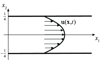
Figure 18: Decaying planar Navier–Stokes flow in a channel with no-slip walls at $x_{2}=\pm\frac{1}{4}$.

The corresponding velocity and scalar vorticity fields are

$$\mathbf{u}(\mathbf{x},t)=e^{-4\pi^{2}\nu t}\left(a\cos 2\pi x_{2},0\right),\qquad\omega(\mathbf{x},t)=2\pi ae^{-4\pi^{2}\nu t}\sin 2\pi x_{2}.$$ (91)

Normalized by their instantaneous global maxima, the normalized linear momentum $\rho\mathbf{u}^{0}=\left(\cos 2\pi x_{2},0\right)$ and vorticity $\omega^{0}=\sin 2\pi x_{2}$ are both constant in time. There is, therefore, no structural reorganization in the topology of the momentum and vorticity fields. Instead, for all times, horizontal lines act as level curves for both the horizontal momentum and the vorticity, forming material barriers between higher and lower values of these scalars. Indeed, the theory developed in this paper identifies all horizontal lines as materiel barriers to the diffusive transport of both momentum and vorticity (see Example 1 of section 7.1).

Haller et al. (2019) obtain an ODE family describing the time $t_{0}$ position of uniform barriers to the diffusive (passive) transport of the scalar vorticity over a finite time interval $[t_{0},t_{1}].$ With the notation $y_{0}=2\pi x_{2}$, with the constants

$$A=\frac{a^{2}}{\nu}\sin 2y_{0}\left[\frac{1}{2}e^{-2\nu t_{1}}+\frac{1}{2}e^{-2\nu t_{0}}-e^{-\nu\left(t_{1}+t_{0}\right)}\right],\qquad B=a\left(e^{-\nu t_{0}}-e^{-\nu t_{1}}\right),$$ (92)

and with the vector field

$$\bar{\mathbf{q}}_{t_{0}}^{t_{1}}(\mathbf{x}_{0})=\frac{1}{2\nu\left(t_{1}-t_{0}\right)}\left(\begin{array}[]{c}A\sin 2y_{0}\\ B\cos y_{0}\end{array}\right),$$ (93)

the ODE family describing the time $t_{0}$ position of uniform constrained barriers is given by

$$\mathbf{x}_{0}^{\prime}=\frac{1}{2\nu\left(t_{1}-t_{0}\right)}\left\{\frac{\sqrt{\left|\mathbf{\bar{q}}_{t_{0}}^{t_{1}}\left(\mathbf{x}_{0}\right)\right|^{2}-\mathcal{T}_{0}^{2}}}{\left|\mathbf{\bar{q}}_{t_{0}}^{t_{1}}\left(\mathbf{x}_{0}\right)\right|^{2}}\left(\begin{array}[]{c}A\sin 2y_{0}\\ B\cos y_{0}\end{array}\right)+\frac{\mathcal{T}_{0}}{\left|\mathbf{\bar{q}}_{t_{0}}^{t_{1}}\left(\mathbf{x}_{0}\right)\right|^{2}}\left(\begin{array}[]{c}B\cos y_{0}\\ -A\sin 2y_{0}\end{array}\right)\right\}$$ (94)

for some value of the transport density constant $\mathcal{T}_{0}\in\mathbb{R}$. For the choice

$$\mathcal{T}_{0}=\left|\mathbf{\bar{q}}_{t_{0}}^{t_{1}}\left(\mathbf{x}_{0}\right)\right|_{y_{0}=0}=\frac{B}{2\nu\left(t_{1}-t_{0}\right)},$$ (95)

the ODE (94) becomes

$$\mathbf{x}_{0}^{\prime} |_{y_{0}=0}=\frac{B}{2\nu\left(t_{1}-t_{0}\right)}\left(\begin{array}[]{c}B\\ 0\end{array}\right)\parallel\mathbf{\bm{\Omega}}\mathbf{\bar{q}}_{t_{0}}^{t_{1}}\left(\mathbf{x}_{0}\right)|_{y_{0}=0},$$ (98)

showing that $x_{02}=0$ is an invariant line for equation (94) for the parameter value $\mathcal{T}_{0}$ selected as in (95). Consequently, the center line of the channel at $x_{02}=0$ is a uniform, constrained barrier to vorticity-diffusion along which the pointwise diffusive transport of vorticity is equal to (94). Choosing the constant $\mathcal{T}_{0}=0$ in eq. (94) gives

$$\mathbf{x}_{0}^{\prime}=\frac{1}{2\nu a\left(t_{1}-t_{0}\right)\left|\mathbf{\bar{q}}_{t_{0}}^{t_{1}}\left(\mathbf{x}_{0}\right)\right|}\left(\begin{array}[]{c}A\sin 4\pi x_{02}\\ B\cos 2\pi x_{02}\end{array}\right),$$ (99)

for which $x_{02}=\pm 1/4$ are invariant lines, and hence the channel walls at $x_{02}=\pm 1/4$ are perfect constrained barriers to diffusive transport. Therefore, the variational theory of Haller et al. (2019) identifies the center line of the channel at $x_{2}=0$ and the upper and lower walls as barriers to vorticity transport, but finds an infinite family of non-straight barrier curves for the rest of the channel, given by general integral curves of the vector field family (94) (see Fig. 1). Only in the limit of $t_{1}\to\infty$ do the latter, curved variational barriers align with horizontal lines, which is suboptimal, given that these horizontal barriers prevail already in any finite-time observation of the vorticity field. The objective of the present paper is to strengthen these results by considering vorticity transport as an active, vectorial transport problem consistent with the 3D Navier–Stokes equation, rather than a passive scalar transport problem in the 2D Navier–Stokes equation.

In contrast, Meyers & Meneveau (2013) define a momentum flux vector field $\bar{\mathbf{F}}_{m}^{\bm{\zeta}}\left(\mathbf{x},t\right)$ with respect to a unit reference direction vector $\bm{\zeta}\in\mathbb{R}^{3}$ as

$$\bar{\mathbf{F}}_{m}^{\bm{\zeta}}=\left(\bar{\mathbf{u}}\cdot\bm{\zeta}\right)\bar{\mathbf{u}}+\overline{\mathbf{u}^{\prime}\otimes\mathbf{u}^{\prime}}\bm{\zeta}-2\nu\bar{\mathbf{S}}\bm{\zeta},$$ (100)

where overbar refers to Reynolds-averaging, prime refers to the fluctuating part of the velocity field, $\otimes$ denotes the dyadic product and $\mathbf{S}=\frac{1}{2}\left[\bm{\nabla}\mathbf{u}+\mathbf{\left(\bm{\nabla}\mathbf{u}\right)}^{T}\right]$ is the rate-of-strain tensor. The flux vector $\bar{\mathbf{F}}_{m}^{\bm{\zeta}}$ is obtained by Meyers & Meneveau (2013) after averaging the unsteady terms out of the Navier–Stokes equations, projecting these averaged equations into the $\bm{\zeta}$ direction, identifying all terms that are divergences of some vector field in these projected equations, and summing up all three vector fields identified in this fashion. For the laminar velocity field (91), we have $\bar{\mathbf{u}}\equiv\mathbf{u}$, $\bar{\mathbf{S}}\equiv\mathbf{S}$, $\mathbf{u}^{\prime}\equiv\mathbf{0}$, and $\bar{\mathbf{F}}_{m}^{\bm{\zeta}}\equiv\mathbf{F}_{m}^{\bm{\zeta}}$. Following the choice of Meyers & Meneveau (2013) for planar parallel shear flows, we select $\bm{\zeta}=\left(1,0\right)^{T}$. Using the relation

$$\mathbf{S}=ae^{-4\pi^{2}\nu t}\left(\begin{array}[]{cc}0&-\pi\sin 2\pi x_{2}\\ -\pi\sin 2\pi x_{2}&0\end{array}\right),$$ (101)

we obtain from eq. (100) the momentum-flux vector

$$\mathbf{F}_{m}^{\bm{\zeta}} =a^{2}e^{-8\pi^{2}\nu t}\left(\begin{array}[]{c}\cos^{2}2\pi x_{2}\\ 0\end{array}\right)-2\nu ae^{-4\pi^{2}\nu t}\left(\begin{array}[]{c}0\\ -\pi\sin 2\pi x_{2}\end{array}\right)$$ (106)

$$=ae^{-4\pi^{2}\nu t}\left(\begin{array}[]{c}ae^{-4\pi^{2}\nu t}\cos^{2}2\pi x_{2}\\ 2\nu\pi\sin 2\pi x_{2}\end{array}\right).$$ (109)

The $x_{2}=0$ line is an integral curve of $\mathbf{F}_{m}^{\bm{\zeta}}$, correctly conveying the fundamental role of the centerline of the channel in blocking linear momentum transfer. All other integral curves of $\mathbf{F}_{m}^{\bm{\zeta}}\left(\mathbf{x},t\right)$, however, curl either upwards or downwards, running eventually into the two horizontal walls perpendicularly. These curves turn very slowly towards to channel walls for small values of the viscosity. For easy illustration over a shorter horizontal domain, we select the time $t^{*}=-\frac{1}{4\pi^{2}\nu}\log\left[2\nu\pi/a\right]$ so that $\mathbf{F}_{m}^{\bm{\zeta}}$ becomes

$$\mathbf{F}_{m}^{\bm{\zeta}}\left(\mathbf{x},t^{*}\right)=2\nu\pi ae^{-4\pi^{2}\nu t^{*}}\left(\begin{array}[]{c}\cos^{2}2\pi x_{2}\\ \sin 2\pi x_{2}\end{array}\right),$$ (110)

whose integral curves are shown in Fig. 1). These integral curves do not delineate observable structures governing the rearrangement of momentum within this flow. In the limit of $t\to\infty,$ they limit on vertical lines.

Appendix B Reynolds transport theorem and the convective flux through the boundary of a material volume

The Reynolds transport theorem for an arbitrary vector field $\mathbf{f}(\mathbf{x},t)$ and an arbitrary, time-varying volume $V(t)$ in a velocity field $\mathbf{u}(\mathbf{x},t)$ is of the form

$$\frac{d}{dt}\int_{V(t)}\mathbf{f}\,dV=\int_{V(t)}\frac{\partial\mathbf{f}}{\partial t}\,dV+\int_{\partial V(t)}\mathbf{f}\left(\mathbf{u}_{\partial V(t)}\cdot\mathbf{n}\right)\,dA.$$ (111)

Here $\mathbf{u}_{\partial V(t)}$ denotes the local velocity of the boundary surface $\partial V(t)$ of $V(t)$, therefore we have $\mathbf{u}_{\partial V(t)}=\mathbf{u}$ when $V(t)$ is a material volume. The identity (111) merely gives a formal partition of $\frac{d}{dt}\int_{V(t)}\mathbf{f}\,dV$ into two terms, yet it is tempting to conclude that the second term, $\int_{\partial V(t)}\mathbf{f}\left(\mathbf{u}\cdot\mathbf{n}\right)\,dA$, is the convective flux of $\mathbf{f}$ through the boundary $\partial V(t)$ of $V(t)$. We will now illustrate on a specific example that this is generally not the case.

Consider the scalar version of 111 for a passive scalar field $c\left(\mathbf{x},t\right)$:

$$\frac{d}{dt}\int_{V(t)}c\,dV=\int_{V(t)}\frac{\partial c}{\partial t}\,dV+\int_{\partial V(t)}c\left(\mathbf{u}\cdot\mathbf{n}\right)\,dA.$$ (112)

Assume that $\mathbf{u}$ is incompressible and $c$ is a passive scalar field that is a solution of the advection-diffusion equation

$$\frac{Dc}{Dt}=\partial_{t}c+\bm{\nabla}c\cdot\mathbf{u}=\kappa\Delta c,$$ (113)

with diffusivity $\kappa>0$. The surface integral in (112) gives a formal convective flux for the passive scalar field $\mathbf{c}$ across $\partial V(t)$ even though no convective scalar transport can occur through the material surface $\partial V(t)$.

The (purely diffusive) flux of $c$ out of $V(t)$ can be computed directly as

$$\frac{d}{dt}\int_{V(t)}c\,dV=\int_{V(t_{0})}\frac{Dc}{Dt}\,dV_{0}=\int_{V(t_{0})}\kappa\Delta c\,dV_{0}=\kappa\int_{V(t)}\bm{\nabla}\cdot\left(\bm{\nabla}c\right)\,dV=\int_{\partial V(t)}\kappa\mathbf{\bm{\nabla}}c\cdot\mathbf{n}\,dA,$$ (114)

showing that the vector describing the correct pointwise diffusive flux vector of the passive scalar $c(\mathbf{x},t)$ through the material surface $\partial V(t)$ is the well-known flux vector, $\kappa\mathbf{\bm{\nabla}}c$ rather than the vector $c\mathbf{u}$ appearing in the surface integral term in (112). This is because the volume integral term $\int_{V(t)}\frac{\partial c}{\partial t}\,dV$ on the right-hand side of the transport theorem (112) also contributes to the flux through $\partial V(t)$. Indeed, using eq. (113), we can rewrite this term as

$$\int_{V(t)}\frac{\partial c}{\partial t}\,dV =\int_{V(t)}\left(\kappa\Delta c-\bm{\nabla}c\cdot\mathbf{u}\right)\,dV=\int_{V(t)}\mathbf{\bm{\nabla}}\cdot\left(\kappa\bm{\nabla}c-c\mathbf{u}\right)\,dV$$

$$=\int_{\partial V(t)}\left(\kappa\bm{\nabla}c-c\mathbf{u}\right)\cdot\mathbf{n}dA.$$ (115)

Therefore, $\int_{V(t)}\frac{\partial c}{\partial t}\,dV$ yields a nonzero flux through the boundary and a part of this flux cancels out the second integral in (112) that incorrectly suggests nonzero convective flux for $c$.

More generally, the partition of $\frac{d}{dt}\int_{V(t)}\mathbf{f}\,dV$ in (111) into two terms is somewhat arbitrary from the point of view of transport through the boundary of a material volume. Indeed, the volume integral on the right-hand-side of (111) will also contribute to the flux of $\mathbf{f}$ through the boundary of $V(t)$.

Appendix C Poofs of Theorems 6 and 7

C.1 Proof of Theorem 6

For a Navier-Stokes velocity field $\mathbf{u}$ of the form (42)-(45), we have

$$\Delta\mathbf{u}\left(\mathbf{x},t\right)=\left(\begin{array}[]{c}\Delta_{\hat{\mathbf{x}}}\hat{\mathbf{u}}\\ \Delta_{\hat{\mathbf{x}}}\hat{\omega}\end{array}\right).$$ (116)

Therefore,

$$\left(\mathbf{F}_{t_{0}}^{t}\right)^{*}\Delta\mathbf{u}(\mathbf{x}_{0}) =\left[\nabla_{\mathbf{x}_{0}}\mathbf{F}_{t_{0}}^{t}\left(\mathbf{x}_{0}\right)\right]^{-1}\left(\begin{array}[]{c}\Delta_{\hat{\mathbf{x}}}\hat{\mathbf{u}}\\ \Delta_{\hat{\mathbf{x}}}\hat{\omega}(\hat{\mathbf{x}},t)\end{array}\right)$$ (119)

$$=\left(\begin{array}[]{cc}\bm{\nabla}_{\mathbf{\hat{\mathbf{x}}}}\hat{\mathbf{F}}_{t}^{t_{0}}\left(\mathbf{\hat{\mathbf{x}}}\right)&\mathbf{0}\\ \int_{t}^{t_{0}}\bm{\nabla}_{\mathbf{\hat{\mathbf{x}}}}\hat{\omega}\left(\hat{\mathbf{F}}_{t}^{s}\left(\hat{\mathbf{x}}\right),s\right)ds&1\end{array}\right)\left(\begin{array}[]{c}\Delta_{\hat{\mathbf{x}}}\hat{\mathbf{u}}\\ \Delta_{\hat{\mathbf{x}}}\hat{\omega}(\hat{\mathbf{x}},t)\end{array}\right)$$ (124)

$$=\left(\begin{array}[]{c}\bm{\nabla}_{\mathbf{\hat{\mathbf{x}}}}\hat{\mathbf{F}}_{t}^{t_{0}}\left(\mathbf{\hat{\mathbf{x}}}\right)\Delta_{\hat{\mathbf{x}}}\hat{\mathbf{u}}\\ \int_{t}^{t_{0}}\bm{\nabla}_{\mathbf{\hat{\mathbf{x}}}}\hat{\omega}\left(\hat{\mathbf{F}}_{t}^{s}\left(\hat{\mathbf{x}}\right),s\right)ds\cdot\Delta_{\hat{\mathbf{x}}}\hat{\mathbf{u}}+\Delta_{\hat{\mathbf{x}}}\hat{\omega}(\hat{\mathbf{x}},t)\end{array}\right).$$ (127)

With these expressions, the barrier equation (21) becomes

$$\hat{\mathbf{x}}_{0}^{\prime} =\nu\rho\overline{\left(\hat{\mathbf{F}}_{t_{0}}^{t}\right)^{*}\Delta_{\hat{\mathbf{x}}}\hat{\mathbf{u}}(\hat{\mathbf{x}}_{0})},$$

$$x_{03}^{\prime} =\nu\rho A(\mathbf{\hat{\mathbf{x}}}_{0},t_{1},t_{0}),$$ (128)

for an appropriate smooth function $A(\mathbf{\hat{\mathbf{x}}}_{0},t_{1},t_{0}).$ Two-dimensional invariant manifolds of this dynamical system are of the form $\left\{\hat{\mathbf{x}}_{0}(s)\right\}_{s\in\mathbb{R}}\times\mathbb{R}$, i.e., topological products of trajectories of the $\hat{\mathbf{x}}_{0}$-component of the (61) with a line in the $x_{03}$ direction. As trajectories $\left\{\hat{\mathbf{x}}_{0}(s)\right\}_{s\in\mathbb{R}}$ are contained in the streamlines of the steady 2D velocity field $\overline{\left(\hat{\mathbf{F}}_{t_{0}}^{t}\right)^{*}\Delta_{\hat{\mathbf{x}}}\hat{\mathbf{u}}(\hat{\mathbf{x}}_{0})}$, Eulerian barriers to momentum transport are, structurally stable streamlines of the vector field $\mathbf{\Delta_{\hat{\mathbf{x}}}\hat{\mathbf{u}}}(\hat{\mathbf{x}},t)$. By incompressibility, we have

$$\Delta_{\hat{\mathbf{x}}}\hat{\mathbf{u}}=\left(\begin{array}[]{c}\partial_{x_{1}x_{1}}^{2}v_{1}+\partial_{x_{2}x_{2}}^{2}v_{1}\\ \partial_{x_{1}x_{1}}^{2}v_{2}+\partial_{x_{2}x_{2}}^{2}v_{2}\end{array}\right)=\left(\begin{array}[]{c}-\partial_{x_{1}x_{2}}^{2}v_{2}+\partial_{x_{2}x_{2}}^{2}v_{1}\\ \partial_{x_{1}x_{1}}^{2}v_{2}-\partial_{x_{1}x_{2}}^{2}v_{1}\end{array}\right)=\left(\begin{array}[]{c}\partial_{x_{2}}\hat{\omega}\\ -\partial_{x_{1}}\hat{\omega}\end{array}\right),$$ (129)

and hence these streamlines are structurally stable level curves of the stream function $\hat{\omega}(\bm{\hat{\mathbf{x}}},t)$, as claimed.

Using formula (129) and the canonical symplectic matrix $\mathbf{J=}\left(\begin{array}[]{cc}0&1\\ -1&0\end{array}\right)$, we also find that

$$\Delta_{\hat{\mathbf{x}}}\hat{\mathbf{u}}\left(\hat{\mathbf{F}}_{t_{0}}^{t}\left(\mathbf{x}_{0}\right),t\right)=\mathbf{J}\bm{\nabla}\omega\left(\hat{\mathbf{F}}_{t_{0}}^{t}\left(\mathbf{x}_{0}\right),t\right)=\mathbf{J}\left[\bm{\nabla}_{0}\hat{\mathbf{F}}_{t_{0}}^{t}\left(\mathbf{x}_{0}\right)\right]^{-T}\bm{\nabla}_{0}\hat{\omega}\left(\hat{\mathbf{F}}_{t_{0}}^{t}\left(\mathbf{x}_{0}\right),t\right),$$ (130)

where $\bm{\nabla}_{0}\hat{\omega}\left(\hat{\mathbf{F}}_{t_{0}}^{t}\left(\mathbf{x}_{0}\right),t\right)$ denotes the derivative of the Lagrangian vorticity $\omega\left(\hat{\mathbf{F}}_{t_{0}}^{t}\left(\mathbf{x}_{0}\right),t\right)$ with respect to the initial condition $\mathbf{x}_{0}$. This last equation implies

$$\left(\hat{\mathbf{F}}_{t_{0}}^{t}\right)^{*}\Delta_{\hat{\mathbf{x}}}\hat{\mathbf{u}}(\mathbf{x}_{0}) =\left[\bm{\nabla}_{0}\hat{\mathbf{F}}_{t_{0}}^{t}\left(\mathbf{x}_{0}\right)\right]^{-1}\Delta_{\hat{\mathbf{x}}}\hat{\mathbf{u}}\left(\hat{\mathbf{F}}_{t_{0}}^{t}\left(\mathbf{x}_{0}\right),t\right)$$

$$=\left[\bm{\nabla}_{0}\hat{\mathbf{F}}_{t_{0}}^{t}\left(\mathbf{x}_{0}\right)\right]^{-1}\mathbf{J}\left[\bm{\nabla}_{0}\hat{\mathbf{F}}_{t_{0}}^{t}\left(\mathbf{x}_{0}\right)\right]^{-T}\bm{\nabla}_{0}\hat{\omega}\left(\hat{\mathbf{F}}_{t_{0}}^{t}\left(\mathbf{x}_{0}\right),t\right)$$

$$=\det\left[\bm{\nabla}_{0}\hat{\mathbf{F}}_{t_{0}}^{t}\left(\mathbf{x}_{0}\right)\right]^{-1}\mathbf{J}\bm{\nabla}_{0}\hat{\omega}\left(\hat{\mathbf{F}}_{t_{0}}^{t}\left(\mathbf{x}_{0}\right),t\right)=\mathbf{J}\bm{\nabla}_{0}\hat{\omega}\left(\hat{\mathbf{F}}_{t_{0}}^{t}\left(\mathbf{x}_{0}\right),t\right),$$ (131)

given that $\det\left[\bm{\nabla}_{0}\hat{\mathbf{F}}_{t_{0}}^{t}\left(\mathbf{x}_{0}\right)\right]^{-1}\equiv 1$ holds due to incompressibility. Here, we have also used the fact here for any constants $a,b,c,d\in\mathbb{R}$ satisfying $ad-bc=1,$ we have

$$\left(\begin{array}[]{cc}a&b\\ c&d\end{array}\right)\left(\begin{array}[]{cc}0&1\\ -1&0\end{array}\right)\left(\begin{array}[]{cc}a&c\\ b&d\end{array}\right)=\left(\begin{array}[]{cc}0&ad-bc\\ bc-ad&0\end{array}\right).$$ (132)

Consequently, we have

$$\overline{\left(\hat{\mathbf{F}}_{t_{0}}^{t}\right)^{*}\Delta_{\hat{\mathbf{x}}}\hat{\mathbf{u}}}(\hat{\mathbf{x}}_{0})=\mathbf{J}\bm{\nabla}_{0}\overline{\hat{\omega}\left(\hat{\mathbf{F}}_{t_{0}}^{t}\left(\hat{\mathbf{x}}_{0}\right),t\right)},$$ (133)

and hence the averaged Lagrangian vorticity $\overline{\hat{\omega}\left(\hat{\mathbf{F}}_{t_{0}}^{t}\left(\mathbf{x}_{0}\right),t\right)}$ acts as an autonomous Hamiltonian (or steady stream function) for the $\hat{\mathbf{x}}_{0}$-component of eq. (128), as claimed in formula (47). Consequently, initial positions of material barriers to momentum transport are level curves of the time-averaged Lagrangian vorticity $\overline{\omega\left(\hat{\mathbf{F}}_{t_{0}}^{t}\left(\mathbf{x}_{0}\right),t\right)}$, as claimed. Furthermore, the instantaneous limit of eq. (47) is (48) and, accordingly, Eulerian barriers to momentum transport are level curves of the Hamiltonian $\hat{\omega}\left(\mathbf{x},t\right)$

C.2 Poof of Theorem 7

For $\mathbf{u}$ defined in (42) and (45), the full vorticity of the 3D flow is given by

$$\bm{\mathbf{\omega}}(\mathbf{x},t)=\left(\partial_{x_{2}}\hat{\omega}(\bm{\hat{\mathbf{x}}},t),-\partial_{x_{1}}\hat{\omega}(\bm{\hat{\mathbf{x}}},t),\hat{\omega}(\bm{\hat{\mathbf{x}}},t)\right),$$ (134)

implying

$$\Delta\bm{\omega}=\left(\begin{array}[]{c}\partial_{x_{2}}\Delta_{\bm{\hat{\mathbf{x}}}}\hat{\omega}\\ -\partial_{x_{1}}\Delta_{\bm{\hat{\mathbf{x}}}}\hat{\omega}\\ \Delta_{\bm{\hat{\mathbf{x}}}}\hat{\omega}\end{array}\right).$$ (135)

In all $x_{3}=const.$ planes, therefore, the vector field $\Delta\bm{\omega}$ admits the same reduced Hamiltonian dynamics, with the Hamiltonian $H=\Delta_{\bm{\hat{\mathbf{x}}}}\hat{\omega}=\frac{1}{\nu}\frac{D}{Dt}\hat{\omega}$ acting as the stream function in that plane. With the notation $\mathbf{J=}\left(\begin{array}[]{cc}0&1\\ -1&0\end{array}\right)$ , we use the calculations in (127) to obtain

$$\left(\mathbf{F}_{t_{0}}^{t}\right)^{*}\Delta\bm{\omega}(\mathbf{x}_{0}) =\left(\begin{array}[]{c}\bm{\nabla}_{\mathbf{\hat{\mathbf{x}}}}\hat{\mathbf{F}}_{t}^{t_{0}}\left(\mathbf{\hat{\mathbf{x}}}\right)\mathbf{J}\bm{\nabla}_{\mathbf{\hat{\mathbf{x}}}}\frac{1}{\nu}\frac{D}{Dt}\hat{\omega}\left(\hat{\mathbf{F}}_{t_{0}}^{t}\left(\hat{\mathbf{x}}_{0}\right),t\right)\\ \int_{t}^{t_{0}}\bm{\nabla}_{\mathbf{\hat{\mathbf{x}}}}\hat{\omega}\left(\hat{\mathbf{F}}_{t}^{s}\left(\hat{\mathbf{x}}\right),s\right)ds\cdot\mathbf{J}\bm{\nabla}_{\mathbf{\hat{\mathbf{x}}}}\frac{1}{\nu}\frac{D}{Dt}\hat{\omega}\left(\hat{\mathbf{F}}_{t_{0}}^{t}\left(\hat{\mathbf{x}}_{0}\right),t\right)+\frac{1}{\nu}\frac{D}{Dt}\hat{\omega}\left(\hat{\mathbf{F}}_{t_{0}}^{t}\left(\hat{\mathbf{x}}_{0}\right),t\right)\end{array}\right).$$ (138)

As a consequence, the first two components of the vorticity barrier equation (39) are

$$\tilde{\mathbf{x}}_{0}^{\prime} =\nu\overline{\bm{\nabla}_{\mathbf{\hat{\mathbf{x}}}}\hat{\mathbf{F}}_{t}^{t_{0}}\left(\mathbf{\hat{\mathbf{x}}}\right)\mathbf{J}\bm{\nabla}_{\mathbf{\hat{\mathbf{x}}}}\frac{D}{Dt}\hat{\omega}\left(\hat{\mathbf{F}}_{t_{0}}^{t}\left(\hat{\mathbf{x}}_{0}\right),t\right)}$$

$$=\nu\overline{\bm{\nabla}_{\mathbf{\hat{\mathbf{x}}}}\hat{\mathbf{F}}_{t}^{t_{0}}\left(\mathbf{\hat{\mathbf{x}}}\right)\mathbf{J}\left[\bm{\nabla}_{\mathbf{\hat{\mathbf{x}}}}\hat{\mathbf{F}}_{t}^{t_{0}}\left(\mathbf{\hat{\mathbf{x}}}\right)\right]^{T}\bm{\nabla}_{\hat{\mathbf{x}}_{0}}\frac{D\hat{\omega}}{Dt}\left(\hat{\mathbf{F}}_{t_{0}}^{t}\left(\hat{\mathbf{x}}_{0}\right),t\right)}.$$ (139)

Using formula (132) again, we obtain from (139) that 2D Lagrangian vorticity-diffusion barriers must satisfy

$$\hat{\mathbf{x}}_{0}^{\prime}=\nu\mathbf{J}\bm{\nabla}_{\hat{\mathbf{x}}_{0}}H_{t_{0}}^{t_{1}}\left(\hat{\mathbf{x}}_{0}\right),\qquad H_{t_{0}}^{t_{1}}\left(\hat{\mathbf{x}}_{0}\right)=\frac{\delta\hat{\omega}\left(\hat{\mathbf{x}}_{0},t_{0},t_{1}\right)}{t_{1}-t_{0}},$$ (140)

as claimed in formula (50), with $H_{t_{0}}^{t_{1}}\left(\hat{\mathbf{x}}_{0}\right)$ playing the role of a Hamiltonian for the two-dimensional $\hat{\mathbf{x}}_{0}$-component of the full material barrier equation, which is therefore of the general form

$$\hat{\mathbf{x}}_{0}^{\prime} =\nu\mathbf{J}\bm{\nabla}_{\hat{\mathbf{x}}_{0}}H_{t_{0}}^{t_{1}}\left(\hat{\mathbf{x}}_{0}\right),$$

$$x_{03}^{\prime} =\nu B(\mathbf{\hat{\mathbf{x}}}_{0},t_{1},t_{0}),$$ (141)

for an appropriate scalar-valued function $G_{t_{0}}^{t_{1}}(\hat{\mathbf{x}}_{0})$. As trajectories $\left\{\hat{\mathbf{x}}_{0}(s)\right\}_{s\in\mathbb{R}}$ are contained in the level curves of the Hamiltonian $H_{t_{0}}^{t_{1}}\left(\hat{\mathbf{x}}_{0}\right)$, we obtain the statement of Theorem 7, using the definition of $H_{t_{0}}^{t_{1}}$ from (140).

Appendix D Proof of Theorem 9

To identify barrier equations for directionally steady Beltrami flows, note that the flow map for the particle motion ODE

$$\dot{\mathbf{x}}=\alpha(t)\mathbf{u}_{0}(\mathbf{x}),\qquad\alpha(t)=e^{-\nu k^{2}\left(t-t_{0}\right)},$$ (142)

of any such flow can be computed from the flow map $\mathbf{G}_{t_{0}}^{\tau}(\mathbf{x}_{0})$ of the autonomous ODE $\dot{\mathbf{x}}=\mathbf{u}_{0}(\mathbf{x})$ as

$$\mathbf{F}_{t_{0}}^{t}(\mathbf{x}_{0})=\mathbf{G}_{t_{0}}^{\tau(t)}\left(\mathbf{x}_{0}\right)=\mathbf{G}_{t_{0}}^{\int_{t_{0}}^{t}\alpha(s)\,ds}\left(\mathbf{x}_{0}\right),$$ (143)

as one verifies by direct substitution of this $\mathbf{F}_{t_{0}}^{t}(\mathbf{x}_{0})$ into (142). Since $\dot{\mathbf{x}}=\mathbf{u}_{0}(\mathbf{x})$ is an autonomous ODE, $\bm{\mathbf{u}}_{0}(\mathbf{F}_{t_{0}}^{t}(\mathbf{x}_{0}))=\bm{\mathbf{u}}_{0}\left(\mathbf{G}_{t_{0}}^{\tau}\left(\mathbf{x}_{0}\right)\right)$ is a solution of its equation of variations, i.e.,

$$\bm{\mathbf{u}}_{0}\left(\mathbf{G}_{t_{0}}^{\tau}\left(\mathbf{x}_{0}\right)\right)=\bm{\nabla}\mathbf{G}_{t_{0}}^{\tau}\left(\mathbf{x}_{0}\right)\bm{\mathbf{u}}_{0}\left(\mathbf{x}_{0}\right).$$ (144)

This implies

$$\bm{\mathbf{u}}_{0}\left(\mathbf{G}_{t_{0}}^{\int_{t_{0}}^{t}\alpha(s)\,ds}\left(\mathbf{x}_{0}\right)\right)=\bm{\nabla}\mathbf{G}_{t_{0}}^{\int_{t_{0}}^{t}\alpha(s)\,ds}\left(\mathbf{x}_{0}\right)\bm{\mathbf{u}}_{0}\left(\mathbf{x}_{0}\right),$$ (145)

or, equivalently, by (143),

$$\bm{\mathbf{u}}_{0}\left(\mathbf{F}_{t_{0}}^{t}(\mathbf{x}_{0})\right)=\bm{\nabla}\mathbf{F}_{t_{0}}^{t}(\mathbf{x}_{0})\bm{\mathbf{u}}_{0}\left(\mathbf{x}_{0}\right).$$ (146)

Multiplying both sides of this equation by $\alpha(t)$ leads to the identity.

$$\left[\bm{\nabla}\mathbf{F}_{t_{0}}^{t}(\mathbf{x}_{0})\right]^{-1}\left(\alpha(t)\bm{\mathbf{u}}_{0}(\mathbf{F}_{t_{0}}^{t}(\mathbf{x}_{0}))\right)=\alpha(t)\bm{\mathbf{u}}_{0}(\mathbf{x}_{0}).$$ (147)

As a consequence of the relation (147), for a directionally steady, strong Beltrami flow, the linear momentum barrier equation (27) takes the specific form

$$\mathbf{x}_{0}^{\prime} =\mathbf{b}_{t_{0}}^{t_{1}}=\nu\rho\,\overline{\left(\mathbf{F}_{t_{0}}^{t}\right)^{*}\Delta\mathbf{u}}=-\nu\rho\overline{\left(\mathbf{F}_{t_{0}}^{t}\right)^{*}\alpha k^{2}\mathbf{u}_{0}}$$

$$=-\frac{\nu\rho}{t_{1}-t_{0}}\int_{t_{0}}^{t_{1}}k^{2}\left[\bm{\nabla}\mathbf{F}_{t_{0}}^{t}(\mathbf{x}_{0})\right]^{-1}\left(\alpha(t)\bm{\mathbf{u}}_{0}(\mathbf{F}_{t_{0}}^{t}(\mathbf{x}_{0}))\right)\,dt$$

$$=-\frac{\nu\rho\int_{t_{0}}^{t_{1}}k^{2}\alpha(t)\,dt}{t_{1}-t_{0}}\bm{\mathbf{u}}_{0}(\mathbf{x}_{0}).$$ (148)

After rescaling the independent variable $s$ in this ODE as $s\to s\frac{t_{0}-t_{1}}{\nu\rho\int_{t_{0}}^{t_{1}}k^{2}\alpha(t)\,dt}$, we obtain the Lagrangian and Eulerian momentum barrier equations

$$\mathbf{x}_{0}^{\prime} =\bm{\mathbf{u}}_{0}(\mathbf{x}_{0}),$$

$$\mathbf{x}^{\prime} =\bm{\mathbf{u}}_{0}(\mathbf{x}).$$ (149)

Note that all invariant manifolds of this barrier equation coincide with invariant manifolds of the particle motion (142) of the directionally steady Beltrami flow defined by (142), which proves the statement of Theorem 9 for linear momentum barriers.

With the relation (147), the vorticity barrier equation (39) for directionally steady Beltrami flows takes the specific form

$$\mathbf{x}_{0}^{\prime} =\mathbf{b}_{t_{0}}^{t_{1}}=\nu\,\overline{\left(\mathbf{F}_{t_{0}}^{t}\right)^{*}\Delta\bm{\omega}}=-\nu\,\overline{\left(\mathbf{F}_{t_{0}}^{t}\right)^{*}\bm{\nabla}\times\left(\bm{\nabla}\times\bm{\omega}\right)}=-\nu\overline{\left(\mathbf{F}_{t_{0}}^{t}\right)^{*}\alpha(t)k^{3}\mathbf{u}_{0}},$$

$$=-\frac{\nu}{t_{1}-t_{0}}\int_{t_{0}}^{t_{1}}k^{3}\left[\nabla_{0}\mathbf{F}_{t_{0}}^{t}(\mathbf{x}_{0})\right]^{-1}\left(\alpha(t)\bm{\mathbf{u}}_{0}(\mathbf{F}_{t_{0}}^{t}(\mathbf{x}_{0}))\right)\,dt$$

$$=-\frac{\nu\int_{t_{0}}^{t_{1}}k^{3}\alpha(t)\,dt}{t_{1}-t_{0}}\bm{\mathbf{u}}_{0}(\mathbf{x}_{0}).$$ (150)

Again, an appropriate rescaling of time shows that all invariant manifolds of this barrier equation coincide with invariant manifolds of the particle motion (142) of the directionally steady Beltrami velocity field $\mathbf{u}(\mathbf{x},t)$, which proves the statement of Theorem 9 for vorticity barriers.

References

- (1) Arnold, V.I., Mathematical Methods of Classical Mechanics, Springer, New York (1978).
- (2) Adrian, R. J., Meinhart, C. D. & Tomkins, C. D. 2000 Vortex organization in the outer region of the turbulent boundary layer. J. Fluid Mech. 422, 1–54.
- (3) Anghan, C., Dave, S., Saincher, S. & Banerjee, J. 2014 Direct numerical simulation of transitional and turbulent round jets: Evolution of vortical structures and turbulence budget, Phys. Fluids 31, 053606.
- (4) Antuono, M. 2020 Tri-periodic fully three-dimensional analytic solutions for the Navier–Stokes equations. J. Fluid Mech. 890, A23.
- (5) Arnold, V.I. 1978 Mathematical Methods of Classical Mechanics, Springer, New York.
- (6) Arnold, V.I., and Keshin, B.A. 1998 Topological Methods in Hydrodynamics. Springer, New York.
- (7) Aref, H., Blake, J.R., Budisic, M., Cardoso, S.S.S., Cartwright, J.H.E., Clercx, H.J.H., El Omari, K., Feudel, U., Golestanian, L., Gouillart, E., van Heijst, G.F., Krasnopolskaya, T.S., Le Guer, Y., MacKay, R.S., Meleshko, V.V., Metcalfe, G.G., Mezic, I., de Moura, A.P.S., Piro, O., Speetjens, M.F.M., Sturman, R., Thiffeault, J.-C., Tuval, I. 2017 Frontiers of chaotic advection. Rev. Modern Phys. 89, 025007
- (8) Balasuriya, S., Ouellette, N. T., & Rypina, I. 2018 Generalized Lagrangian Coherent Structures, Physica D. 372, 31–51.
- (9) Batchelor, G. K. 2000 An Introduction to Fluid Mechanics. Cambridge University Press, Cambridge.
- (10) Barbato, D., Berselli, L.-C., & Grisanti, C.R. 2007 Analytical and numerical results for the rational large eddy simulation model. J. Math. Fluid Mech. 9, 44–74.
- (11) Bird, R. B., Stewart, W. E., & Lightfoot, E. N. 2007 Transport Phenomena. John Wiley & Sons, New York.
- (12) Childress, S., 2009 A Theoretical Introduction to Fluid Mechanics. AMS, Providence.
- (13) De Silva, C., Hutchins, N., & Marusic, I. 2016 Uniform momentum zones in turbulent boundary layers. J. Fluid Mech., 786, 309-331.
- (14) Dinklage, A. Klinger, T., Marx, G., & Schweikhard, L. 2005 Plasma Physics – Confinement, Transport and Collective Effects. Springer, Berlin.
- (15) Dombre, T., Frisch, U., Greene, J.M., Hénon, M., Mehr, A., & Soward, A.M. 1986 Chaotic streamlines in ABC flows, J. Fluid Mech. 167, 353–391.
- (16) Dubief, Y. & Delcayre, F. 2000 On coherent-vortex identification in turbulence, J. Turbulence 1, 011.
- (17) Ethier, R.C., and Steinman, D.A. 1994 Exact fully 3D Navier–Stokes solutions for benchmarking. Int. J. Num. Methods. Fluids. 19, 369-375.
- (18) Epps, B. 2017 Review of vortex identification methods. in AIAA SciTech Forum, 9-13 January 2017, Grapevine, Texas, 55th AIAA Aerospace Sciences Meeting, 1-22.
- (19) Falahatpisheha, A., Kheradvarc, A., 2015 A measure of axisymmetry for vortex rings. European Journal of Mechanics B/Fluids 49, 264–271.
- (20) Farazmand, M., Kevlahan, N. & Protas, B. 2011 Controlling the dual cascades of two-dimensional turbulence, J. Fluid Mech. 668, 202-222.
- (21) Farazmand, M. & Haller, G. 2016 Polar rotation angle identifies elliptic islands in unsteady dynamical systems. Physica D 315, 1-12.
- (22) Fraenkel, L. E. 1970 On steady vortex rings of small cross-section in an ideal fluid. Proc. Roy. Soc. A. 316, 29.
- (23) Fraenkel, L. E. 1972 Examples of steady vortex rings of small cross-section in an ideal fluid. J . Fluid Mech. 51 (1972) 119.
- (24) Gao, F., Ma, W., Zambonini, G., Boudet, J., Ottavy, X., Lu, L. & Shao, L. 2015 Large-eddy simulation of 3-D corner separation in a linear compressor cascade, Phys. Fluids 27, 085105.
- (25) Guckenheimer, J. & Holmes, P. 1983 Nonlinear Oscillations, Dynamical Systems and Bifurcations of Vector Fields. Springer, New York.
- (26) Gurtin, M.E., Fried, E., & Anand, L. 2013 The Mechanics and Thermodynamics of Continua. Cambridge University Press, Cambridge..
- (27) Günther, T. & Theisel, H. 2018 The state of the art in vortex extraction. Comp. Graphics Forum. 37, 149-173.
- (28) Hadjighasem, A., Farazmand, M., Blazevski, D. Froyland, G. & Haller, G. 2017 A critical comparison of Lagrangian methods for coherent structure detection. Chaos 27, 053104.
- (29) Haller, G.2001 Distinguished material surfaces and coherent structures in 3D fluid flows. Physica D 149, 248-277.
- (30) Haller, G. 2015 Lagrangian Coherent Structures. Annual Rev. Fluid. Mech, 47, 137-162.
- (31) Haller, G., Hadjighasem, A., Farazamand, M., & Huhn, F. 2016 Defining coherent vortices objectively from the vorticity. J. Fluid Mech. 795, 136-173.
- (32) Haller, G., Karrasch, D., & Kogelbauer, F. 2018 Material barriers to diffusive and stochastic transport. Proc. Natl. Acad. Sci. U.S.A.,115/37, 9074-9079.
- (33) Haller, G., Karrasch, D., & Kogelbauer, F., 2020 Barriers to the transport of diffusive scalars in compressible flows, SIAM J. Appl. Dyn. Sys., 85–123.
- (34) Hamilton, J., Kim, J., & Waleffe, F. 1995 Regeneration mechanisms of near-wall turbulence structures. J. Fluid Mech., 287, 317–348.
- (35) Hasegawa, Y., Quadrio, M. & Frohnapfel, B., 2014 Numerical simulation of turbulent duct flows at constant power input, J. Fluid Mech. 750, 191–209.
- (36) Hunt, J. C. R., Wray, A. & Moin, P. 1988 Eddies, stream, and convergence zones in turbulent flows. Center for Turbulence Research Report CTR-S88.
- Hutchins, N. & Marusic, I. (2007) Hutchins, N. & Marusic, I. 2007 Large-scale influences in near-wall turbulence. Phil. Trans.R. Soc. A 365, 647–664.
- (38) Jantzen, R.T., Taira, K., Granlund, K.O. & Ol, M.V. 2019 Vortex dynamics around pitching plates, Phys. Fluids 26, 065105.
- (39) Jeong, J. & Hussain, F. 1995 On the identification of a vortex. J. Fluid Mech. 285, 69–94.
- (40) Jeong, J., Hussain, F., Schoppa, W. & Kim, J. 1997 Coherent structures near the wall in a turbulent channel flow. J. Fluid Mech. 332, 185–214.
- (41) Jiménez, J., & Pinelli, A. 1999 The autonomous cycle of near-wall turbulence. J. Fluid Mech. 389, 335–359.
- (42) Katsanoulis, S., Farazmand, M., Serra, M. & Haller, G. 2020 Vortex boundaries as barriers to diffusive vorticity transport in two-dimensional flows, Phys. Rev. Fluids 5, 024701.
- (43) Kirkwood, J. 2018 Mathematical Physics with Partial Differential Equations. Academic Press, London.
- (44) Lele, S.K. 1992 Compact finite-difference schemes with spectral-like resolution. J. Comp. Phys. 103, 16–42.
- (45) Luchini, P. & Quadrio, M. 2006 A low-cost parallel implementation of direct numerical simulation of wall turbulence. J. Comp. Phys. 211, 551-571.
- (46) Lugt, H.J. 1979 The dilemma of defining a vortex", in Recent Developments in Theoretical and Experimental Fluid Mechanics, U. Muller, K. G. Riesner, and B. Schmidt, (eds.) 13, 309-321.
- (47) MacKay, R.S. 1994 Transport in 3D volume-preserving flow. J. Nonlinear Sci. 4, 329-354.
- (48) Majda, A.J., and Bertozzi, A.L. 2002 Vorticity and Incompressible Flow. Cambridge University Press, Cambridge.
- (49) Marusic, I., Mathis, R. & Hutchins, N. 2010 Predictive model for wall-bounded turbulent flow. Science 329, 193–196.
- (50) Mackay, R.S., Meiss, J. D., & Percival, I.C. 1984 Transport in Hamiltonian systems, Physica D 13 (1984) 55-81.
- (51) McMullan, W.A. & Page, G.J. 2012 Towards Large Eddy Simulation of gas turbine compressors, Progr. in Aerospace. Sci. 52, 30–47.
- (52) Meiss, J. D. 1992 Symplectic maps, variational principles, and transport. Rev. Mod. Phys. 64, 795-848.
- (53) Meyers, J. & Meneveau, C. 2013 Flow visualization using momentum and energy transport tubes and applications to turbulent flow in wind farms. 715, 335–358
- (54) Nolan, P.J., Serra, M. & Ross, S.D. 2020 Finite-time Lyapunov exponents in the instantaneous limit and material transport. Nonlinear Dyn. https://doi.org/10.1007/s11071-020-05713-4
- (55) Norbury, J. 1973 A family of steady vortex rings. J. Fluid Mech. 57, 417-431.
- (56) Ogden, R.W. 1984 Non-linear Elastic Deformations, Ellis Horwood, Chichester..
- (57) Ottino, J.M. 1989 The Kinematics of Mixing: Stretching, Chaos and Transport, Cambridge University Press, Cambridge.
- (58) Pandey, A. Scheel, J.D. & Schumacher, J. 2018 Turbulent superstructures in Rayleigh-Bénard convection, Nature Comm. 9, 2118
- (59) Pedergnana, T., Oettinger, D., Langlois, G. P. & Haller, G. 2020 Explicit unsteady Navier-Stokes solutions and their analysis via local vortex criteria Phys. Fluids 32, 046603.
- (60) Pitton, E., Marchioli, C., Lavezzo, C., Soldati, A. & Toschi, F. 2012 Anisotropy in pair dispersion of inertial particles in turbulent channel, Phys. Fluids 24, 073305.
- (61) Quadrio, M. & Luchini, P. 2003 Integral space–time scales in turbulent wall flows. Phys. Fluids 24 2219-2227
- (62) Robinson, S. K. 1991 Coherent motions in the turbulent boundary layer, Ann. Rev. Fluid Mech. 23, 601–639.
- (63) Rosner, D. 2000 Transport Processes in Chemically Reacting Flow Systems. Dover Publications.
- (64) Saffman, P. G., Ablowitz, M. J., Hinch, E., Ockendon, J. R., & Olver, P. J. 1992. Vortex Dynamics. Cambridge University Press, Cambridge.
- (65) Sadlo, F. & Pikert, R.,], Sadlo, F. & Pikert, R.], Sadlo, F. & Pikert, R., 2009 Visualizing Lagrangian coherent structures and comparison to vector field topology, in Topology-Based Methods in Visualization II, Springer, Berlin Heidelberg, 15-29.
- (66) Schindler, B. Peikert, R., Ruchs, R. & Theisel, H. 2012 Ridge concepts for the visualization of Lagrangian coherent structures, in Topological Methods in Data Analysis and Visualization II: Theory, Algorithms, and Applications, Springer, Berlin Heidelberg, 221-235.
- (67) Serra, M. & Haller, G. 2016 Objective Eulerian coherent structures. Chaos 26, 053110.
- (68) Surana, A., Grunberg, O. & Haller, G. 2006 Exact theory of three-dimensional flow separation. Part I. Steady separation J. Fluid. Mech. 564, 57-103.
- (69) van Hinsberg, M.A.T., Ten Thije Boonkamp, J.H.M., Toschi, F. & Clercx, H.J.H. 2012 On the efficiency and accuracy of interpolation methods for spectral codes, J. Sci. Comput. 34, 479–498.
- (70) Wang, C.Y. 1990 Exact solutions of the Navier-Stokes equations- the generalized Beltrami flows, review and extension. Acta Mechanica 81, 69-74.
- (71) Weiss, J.B. and Provenzale, A. 2008 Transport and Mixing in Geophysical Flows: Creators of Modern Physics 744, Springer, Berlin.