Electron pairing by Coulomb repulsion in narrow band structures

Abstract

Abstract: We study analytically and numerically dynamics and eigenstates of two electrons with Coulomb repulsion on a tight-binding lattice in one and two dimensions. The total energy and momentum of electrons are conserved and we show that for a certain momentum range the dynamics is exactly reduced to an evolution in an effective narrow energy band where the energy conservation forces the two electrons to propagate together through the whole system at moderate or even weak repulsion strength. We argue that such a mechanism of electron pair formation by the repulsive Coulomb interaction is rather generic and that it can be at the origin of unconventional superconductivity in twisted bilayer graphene.

Introduction. - The interactions of electrons in narrow band structures play an important role in various physical processes. Often the theoretical analysis is done in the frame work of electrons on a lattice with short range on-site interactions as described in works of Gutzwiller and Hubbard gutzwiller1963 ; hubbard1963 ; gutzwiller1965 . Recently, the interest to narrow band structures with strong Coulomb electron-electron interactions has been inspired by the observation of unconventional superconductivity in magic-angle twisted bilayer graphene (MATBG) cao2018 . Such structures are characterized by a very high ratio of critical temperature of the superconducting transition to Fermi energy $T_{c}/E_{F}$ cao2018 and complex phase diagrams of superconducting and insulating phases ashoori2018nat ; efetov2019nat . Experimental results for MATBG clearly show the importance of long range Coulomb electron-electron interactions in these structures cao2018 ; ashoori2018nat ; efetov2019nat ; efetovscreen . From the theoretical side it has been shown that for small twisted angles the moiré pattern leads to a formation of a superlattice with a unit cell containing more than 10000 atoms that significantly modifies the low-energy structure. Extensive numerical studies by quantum-chemistry methods show the appearance of flat lowest-energy mini bands flatband1 ; flatband2 ; flatband3 ; flatband4 . These bands are rather narrow and thus the Coulomb interactions play an important role as it was already pointed out in early theoretical studies macdonald . The existence of narrow flat bands is also confirmed in recent MATBG experiments berkeley .

In this Letter we show that the narrow band structure of free electron spectrum leads to a number of unusual properties of their propagation in presence of strong, moderate or even weak Coulomb repulsion between electrons. We discuss these properties on a model of two electrons with Coulomb interaction propagating on a standard tight-binding lattice considered in gutzwiller1963 ; hubbard1963 ; gutzwiller1965 . Our results show the appearance of pairing of two electrons induced by a moderate Coulomb repulsion with ballistic pairs propagating over the whole system size. Below we describe the physical properties of such pairs of two interacting particles (TIP).

Quantum tight-binding model of two electrons. - The quantum Hamiltonian of the model in dimensions $d=1$ or $2$ has the standard form gutzwiller1963 ; hubbard1963 ; gutzwiller1965 :

$$H=-\sum_{\langle j,l\rangle}|j\rangle\langle l|+\sum_{j}\frac{U}{1+r(j)}|j\rangle\langle j|$$ (1)

where $j=(x_{1},x_{2})$ ($j=(x_{1},x_{2},y_{1},y_{2})$) is a multi-index for $d=1$ ($d=2$); each index variable takes values $x_{1},x_{2},y_{1},y_{2}\in\{0,\ldots,N-1\}$ with $N$ being the linear system size with periodic boundary conditions. The first sum in (1) describes the electron hopping between nearby sites on a 1D (or 2D square) lattice with a hopping amplitude taken as energy unit. The second sum in (1) represents a (regularized) Coulomb type long-range interaction with amplitude $U$ and the distance $r(j)$ between two electrons. For 1D we have, due to the periodic boundary conditions, $r(j)=\Delta\bar{x}$ with $\Delta\bar{x}=\min(\Delta x,N-\Delta x)$ and relative coordinate $\Delta x=x_{2}-x_{1}$ which is taken modulo $N$ (i.e. $\Delta x=x_{2}-x_{1}+N$ for $x_{2}-x_{1}<0$). For 2D we have $r(j)=\sqrt{\Delta\bar{x}^{2}+\Delta\bar{y}^{2}}$. Furthermore, we consider symmetric (spatial) wave functions with respect to particle exchange assuming an antisymmetric spin-singlet state (similar results are obtained for antisymmetric wave functions). In absence of interactions at $U=0$ the spectrum of free electrons has the standard band structure $E=-2\sum_{\mu=1,2;\,\alpha}\cos p_{\mu\alpha}$ with $\mu=1,2$ being the electron index and $\alpha=x$ in 1D ($\alpha\in\{x,y\}$ in 2D) being the index for each spatial dimension. With periodic boundary conditions each momentum $p_{\mu\alpha}$ is an integer multiple of $2\pi/N$.

Classical dynamics of electron pairs. - The corresponding classical dynamics in 2D is described by the Hamiltonian:

$$H=-2\sum_{\mu=1,2;\,\alpha\in\{x,y\}}\cos p_{\mu\alpha}+U_{C}(x_{1},x_{2},y_{1},y_{2})$$ (2)

with $U_{C}=U/[1+\sqrt{(x_{1}-x_{2})^{2}+(y_{1}-y_{2})^{2}}]$ and conjugated variables of momentum $p_{\mu x},p_{\mu y}$ and coordinates $x_{\mu},y_{\mu}$ (in 1D we have in (2) only $p_{\mu x}$ and $x_{\mu}$). In 1D there are two integrals of motion being the total energy $E=H$ and total momentum $p_{+}=p_{1x}+p_{2x}$ leading to integrable TIP dynamics. In 2D we have 3 integrals of motion $E,p_{+x},p_{+y}$ for 4 degrees of freedom and therefore the dynamics of the two electrons is generally chaotic as it is shown in Fig. S1 of suppmat , Sec. S1.

Writing $\cos(p_{1x})+\cos(p_{2x})=2\cos(p_{+x}/2)\cos[(p_{2x}-p_{1x})/2]$ (and similarly for $y$) we see that at given values of $p_{+x},p_{+y}$ the kinetic energy is bounded by $\Delta E=4\sum_{\alpha}|\cos(p_{+\alpha}/2)|$. Therefore for TIP states with $E>\Delta E$ the two electrons cannot separate and they propagate as one pair. In particular for $p_{+x}=p_{+y}=\pi+\delta$ (with $|\delta|\ll 1$) being close to $\pi$ there are compact Coulomb electron pairs even for very small interactions $U$ as soon as $\Delta E\approx 2d|\delta|<U\ll B_{d}$ with $B_{d}=8d+U$ being the maximal energy bandwidth in $d$ dimensions. The center of mass velocity of such pairs (in direction $\alpha\in\{x,y\}$) is $v_{+\alpha}=(v_{1\alpha}+v_{2\alpha})/2=$ $2\cos(\delta/2)\,\sin(p_{1\alpha}-\delta/2)\approx 2\sin p_{1\alpha}$ and it may be close to a maximal velocity $v_{+\alpha}=2$. Fig. S1 of suppmat clearly confirms the pair formation at small $U$ values and the pair propagation through the whole system.

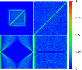
Figure 1: Color plot of wave function amplitudes obtained from the exact quantum time evolution in 1D at times $t=138\,\Delta t$ ($t=10^{5}\Delta t$) in left (right) panels ($\Delta t=1/B_{1}$ is an elementary time step of inverse band width $B_{1}=8+U$). Top panels show the TIP wave function amplitude $|\psi(x_{1},x_{2},t)|$ at $x_{1}$ and $x_{2}$ for both axis. Bottom panels show $|\bar{\psi}(p_{+},\Delta x,t)|$ with $\Delta x=x_{2}-x_{1}$ (taken modulo N) being the relative coordinate (horizontal axis) and $0\leq p_{+}<2\pi$ being the total momentum (vertical axis). The initial state at $t=0$ is a symmetrized state with one electron localized at $N/2$ and the other one at $N/2+1$, i.e. initial distance $\Delta\bar{x}=1$. Other parameters are $U=1$ and $N=128$; color bar represents (here and in certain subsequent figures) the ratio of the shown quantity (here modulus of wave function amplitude) to its maximal value. Related videos are available at suppmat ; ourwebpage .

Quantum TIP eigenstates and dynamics in 1D and 2D. - The factor $2\cos(p_{+}/2)$ for the kinetic energy (in 1D) at given value of $p_{+}$ can also be obtained from the quantum model. Using a suitable unitary transformation (see suppmat , Sec. S2) one can transform the quantum Hamiltonian (1) to a block diagonal form where the different blocks on the diagonal correspond, for each value of the conserved quantum number $p_{+}$, to an effective one-particle tight binding model (in $\Delta x$ space) with nearest neighbor hopping matrix element $-2\cos(p_{+}/2)$ and a diagonal potential given by $U/(1+\Delta\bar{x})$ (see suppmat , Sec. S2 for details, especially the boundary conditions and the generalization to the 2D case). Physically, this corresponds to a single particle in $\Delta x$ space with a kinetic energy rescaled by $2\cos(p_{+}/2)$ and moving in a given potential with maximal value $U$ for $\Delta x$ being close to $0$ or $N$.

The eigenstates can be efficiently calculated for large system sizes since each block for a given value of $p_{+}$ can be diagonalized individually. Also the quantum time evolution (for $\hbar=1$) can be efficiently computed (up to $N=1024$) by transforming the initial state $\psi(x_{1},x_{2})$ into block representation $\bar{\psi}(p_{+},\Delta x)$ and computing the time evolution exactly in each $p_{+}$ sector using the exact block eigenstates (details in suppmat , Sec. S2).

A typical example of the TIP time evolution in 1D is shown in top panels of Fig. 1 for initial electron positions (localized at $x_{\mu}\approx N/2$) at a distance $R=\Delta\bar{x}=1$ for $U=1$ and $N=128$. We see a wave front of free propagating separated electrons (square at small times in top left panel) and at the same time free propagation of the Coulomb electron pair along the diagonal $x_{1}=x_{2}$. At large times the density for separated electrons is uniformly distributed over the whole system while the density for Coulomb pairs is homogeneously distributed over the whole diagonal keeping a relatively small pair size (top right panel). Bottom panels show the block representation $|\bar{\psi}(p_{+},\Delta x,t)|$ of the same states as in top panels. In this representation the initial state corresponds to two red vertical lines at $\Delta x=1$ and $\Delta x=N-1$ for perfect localization at these values and a uniform distribution in $p_{+}$ direction. With increasing time a part of the density stays quite well localized to the initial values with some modest increase of the initial width. The other fraction of the density propagates horizontally and becomes roughly uniform at sufficiently long times. The speed of the horizontal propagation is apparently proportional to $\cos(p_{+}/2)$ and for $p_{+}\approx\pi$ there is actually a small regime of strong, nearly perfect localization, where the weight of the propagating density is close to 0. In this case the kinetic energy can be considered as a small perturbation of the interaction due to the small ratio $2|\cos(p_{+}/2)|/U\ll 1$. However even for larger values of this ratio there is still a considerable fraction of the density that stays localized.

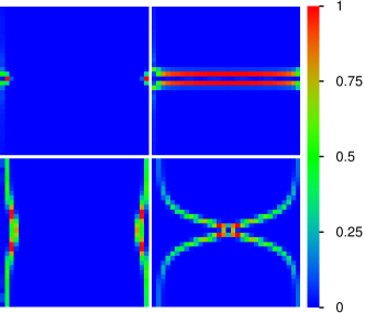
Figure 2: Examples of Husimi functions of symmetrized 1D block eigenstates in relative coordinates $\Delta x\in[0,N[$ ($x$-axis) and corresponding momentum $\Delta p\in[0,2\pi[$ ($y$-axis) in certain $p_{+}$ sectors for $N=1024$, $U=1$. Top (bottom) panels correspond to $p_{+}=341\pi/512\approx 2\pi/3$ ($p_{+}=511\pi/512\approx\pi$). Relative level numbers (ordered by increasing energies) inside each $p_{+}$ sector are 509 (top left), 474 (top right), 464 (bottom left), 374 (bottom right).

Fig. 2 shows certain Husimi functions of 1D block eigenstates obtained from the smoothing of the Wigner function on the scale of $\hbar$ (see e.g. husimi1 ; husimi2 ) for two sectors $p_{+}\approx 2\pi/3$ and $p_{+}\approx\pi$. For larger energies there is a clear localization in $\Delta x$ at $\Delta x\approx 0$ and $\Delta x\approx N$ where the interaction potential is maximal and for medium/lower energies there is a near ballistic movement over the full $\Delta x$ range. For $p_{+}\approx 2\pi/3$ there is also localization in $\Delta p$ with two values close to $\pi$ in top right panel but the typical localized $\Delta p$ value may be different for other eigenstates (not shown) except for the few eigenstates with top energies which are localized in $\Delta x$. For $p_{+}\approx\pi$, where the effective kinetic energy is strongly reduced, there is a larger number of states with localization in $\Delta x$ for larger energies and for all cases $\Delta p$ appears to be rather delocalized. The states with localization in $\Delta x$ contribute mostly in the quantum time evolution shown in Fig. 1 due to the initial localized state at $\Delta x=1$ thus explaining the significant probability for both particles staying together. Further results of the 1D quantum case are given in Figs. S2-S4 of suppmat , Sec. S3.

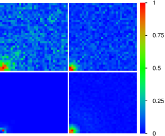
Figure 3: Color plot of wave function amplitude $|\bar{\psi}(p_{+x},p_{+y},\Delta x,\Delta y)|$ in block representation obtained from the 2D quantum time evolution at iteration time $t=10^{5}\Delta t$ in $\Delta x$-$\Delta y$ plane for certain $p_{+x}$, $p_{+y}$ sectors and $U=2$ ($\Delta t=1/B_{2}=1/(16+U)$). The initial block state at $t=0$ is localized at $\Delta x=\Delta y=1$. All panels show a zoomed region $0\leq\Delta x,\Delta y<32$. The values of $p_{+}=p_{+x}=p_{+y}$ and $N$ are $p_{+}=0$, $N=128$ (top left), $p_{+}=21\pi/32\approx 2\pi/3$, $N=128$ (top right), $p_{+}=63\pi/64\approx\pi$, $N=128$ (bottom left), $k=85\pi/128\approx 2\pi/3$, $N=512$ (bottom right). Related videos are available at suppmat ; ourwebpage .

In order to access larger system sizes up to $N=512$ we compute for the 2D case the exact quantum time evolution only in individual sectors with $p_{+x}=p_{+y}$ (and exploiting certain symmetries suppmat ). The initial state is localized at $\Delta\bar{x}=\Delta\bar{y}=1$ but also at the chosen value of $p_{+x}=p_{+y}$. This corresponds to a wave in the center of mass direction with momenta $p_{+x},p_{+y}$ which is however perfectly localized in the relative coordinate.

Fig. 3 clearly shows that there is a considerable probability that both electrons stay together even at very large times. There is however, for $p_{+x,y}=0$ or $p_{+x,y}\approx 2\pi/3$, also a certain complementary density for free electron propagation which becomes less visible for larger $N=512$. For $p_{+x,y}\approx\pi$ there is actually near perfect localization even at $N=128$. This confirms the formation of Coulomb electron pairs in the 2D quantum case and as in 1D also the particularly strong localization in relative coordinates for sectors with $p_{+x,y}\approx\pi$

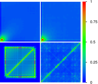
Figure 4: 2D Wave function densities obtained from the time evolution shown at times $t=445\,\Delta t$ ($t=10^{4}\Delta t$) in left (right) panels for initial electron positions at $\approx(N/2,N/2)$ and $N=128$, $U=2$ ($\Delta t=1/B_{2}=1/(16+U)$ is the Trotter integration time step). Top panels show the zoomed density for $0\leq\Delta x,\Delta y<32$ in the $\Delta x$-$\Delta y$ plane of relative coordinates obtained from a sum over $x_{1}$ and $y_{1}$. Bottom panels show the density in $x_{1}$-$x_{2}$ plane obtained from a sum over $y_{1}$ and $y_{2}$. The corresponding value of probability near diagonal $w_{10}$ is $w_{10}=0.106$ ($w_{10}=0.133$) for left (right) panels (see text). Related videos are available at suppmat ; ourwebpage .

We also computed the full space 2D quantum time evolution using the Trotter formula approximation (see e.g. trotter for computational details) with a Trotter time step $\Delta t=1/B_{2}=1/(16+U)=1/18$ for $U=2$ and for $N=128$. Here we choose an initial condition with both particles localized at $\approx(N/2,N/2)$ such hat $\Delta\bar{x}=\Delta\bar{y}=1$. The results of Fig. 4 clearly show that there is a significant probability of electron pair formation with a propagation of pairs over the whole system (high probability of $\Delta x,\Delta y$ at values close to zero in top panels and near the diagonal $x_{1}\approx x_{2}$ in bottom panels). At the same time there is also a certain probability to have practically independent electrons with ballistic propagation through the lattice at moderate times (bottom left panel) and an approximate homogeneous distribution over the whole system at large times (bottom right panel).

In order to characterize the pair formation probability we compute the quantum probability $w_{10}(t)$ to find both electrons at a finite distance from each other $\Delta\bar{x}\leq\Delta R=10$ and $\Delta\bar{y}\leq\Delta R$. At large times we find that the pair formation probability is $w_{10}=0.133$ while the probability to have independent electrons is $1-w_{10}$.

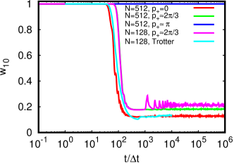
Figure 5: Time dependence of the pair formation probability $w_{10}$ for $U=2$ and different cases of either the exact 2D time evolution in certain sectors of conserved momenta $p_{+}=p_{+x}=p_{+y}$ or the full space 2D time evolution using the Trotter formula approximation (initial states as in Figs. 3,4). The precise values of $p_{+}$ are : $p_{+}=0$, $p_{+}=85\pi/128\approx 2\pi/3$, $p_{+}=255\pi/256\approx\pi$ all three for $N=512$ and $p_{+}=21\pi/32\approx 2\pi/3$ for $N=128$. The top blue line at $w_{10}=1$ is accurate with a numerical error below $10^{-14}$ for all time values.

The time dependence of the pair formation probability $w_{10}$ for both types of 2D quantum time evolution is shown in Fig. 5 for $U=2$ and $N\in\{128,512\}$. For $p_{+}\approx\pi$ we have $w_{10}=1$ with numerical accuracy while for $p_{+}\approx 2\pi/3$ and $p_{+}=0$ this probability decreases with time but saturates at rather high values $w_{10}\approx 0.2$ and $0.13$ respectively. The saturation value $w_{10}\approx 0.133$ for the full space Trotter formula approximation is very close to the case $p_{+}=0$.

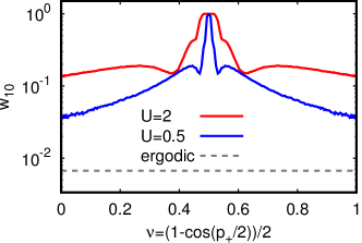
Figure 6: Dependence of pair formation probability $w_{10}$ on the filling factor $\nu$ for $U=2$ (red curve), $0.5$ (blue curve) for $N=256$ in 2D. The dashed line shows the ergodic probability $w_{\rm erg.}$ assuming a uniform wave function.

The initial state with the pair momentum $p_{+}$ approximately corresponds to the electron Fermi energy $E_{F}\approx-4\cos(p_{+}/2)$ assuming relatively moderate or weak interaction $U\ll B_{d}$. Thus the variation of $p_{+}$ in the range $0\leq p_{+}\leq 2\pi$ corresponds to the variation of the filling factor $\nu$ in the range $0\leq\nu\leq 1$ with $\nu=(1-\cos(p_{+}/2))/2$. The dependence $w_{10}(\nu)$ on $\nu$ is shown in Fig. 6 for $U=0.5,\,2$ and $N=256$ (data for $N=512$ is very close). We see that for small $\nu\ll 1/2$ the electron pair formation probability is relatively small but for $1/3\leq\nu\leq 1/2$ it takes for $U=2$ ($U=0.5$) values from $w_{10}=0.17$ ($w_{10}=0.11$) to $w_{10}=1$. The values of $w_{10}$ are significantly above the ergodic probability $w_{\rm erg.}=(21/N)^{2}\approx 0.0067$ for $N=256$ assuming a uniform distribution.

More results for the quantum time evolution and eigenstates properties in 2D are given in suppmat (see Figs. S4-S10 of Sec. S4). In particular, there is a clear scaling dependence of $w_{10}$ (and other related characteristics) on the ratio $2\cos(p_{+}/2)/U$ (Figs. S9, S10 of suppmat )

Discussion. - The presented analytical and numerical analysis definitely shows that a specific energy dispersion law of free electrons in narrow bands leads to a new possibility of pair formation induced by Coulomb repulsion between electrons. The pairing of electrons already exists for a relatively moderate, or even small, repulsion strength $U$. Of course, this analysis is performed in the frame work of only two interacting electrons. However, we conjecture that these Coulomb electron pairs will still exist even at finite electron density $\nu$. Indeed, a propagating pair can feel interactions from other electrons as a certain mean field potential which should not destroy pairs with a relative strong coupling. In presence of an external space inhomogeneous potential the independent electrons can be localized by the potential while the pairs, being protected by their effective coupling energy $\Delta_{c}\sim U/\Delta R$, can remain insensitive to the potential propagating through the whole system (we assume that $\Delta R$ is of the order of several lattice units as for $w_{10}$ computations). Thus such pairs can form a condensate leading to the emergence of a superconducting state. We argue that the emergence of Coulomb electron pairs in narrow band structures can be at the origin of superconductivity in MATBG experiments.

Acknowledgments. - This work was supported in part by the Programme Investissements d’Avenir ANR-11-IDEX-0002-02, reference ANR-10-LABX-0037-NEXT (project THETRACOM). This work was granted access to the HPC resources of CALMIP (Toulouse) under the allocation 2019-P0110.

Appendix A

Supplementary Material for
Electron pairing by Coulomb repulsion in narrow band structures
by K. M. Frahm and D. L. Shepelyansky.

Here, we present additional material for the main part of the article.

Appendix B S1. Classical chaotic dynamics and propagation of two electrons in 2D

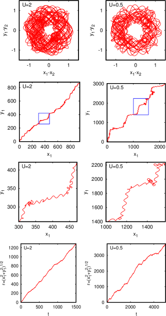
Figure S1: Classical dynamics for 2D case with a classical trajectory obtained by the standard Runge-Kutta 4th order method using a time step of $dt=0.005$. The initial condition corresponds to $|x_{1}-x_{2}|\approx|y_{1}-y_{2}|\approx 1$ and conserved total momenta being $p_{x1}+p_{x2}=p_{y1}+p_{y2}=\pi+\Delta p$ close to $\pi$. Panels of left (right) column correspond to $U=2$, $\Delta p=0.1$ and maximal time $t_{\rm max}=1500$ ($U=0.5$, $\Delta p=0.02$, $t_{\rm max}=5000$). Top panels show the dependence of $y_{1}-y_{2}$ on $x_{1}-x_{2}$; 2nd row of panels show the propagation of $y_{1}$ versus $x_{1}$ and 3rd row of panels provide a zoomed view of the blue rectangles visible in 2nd row panels revealing a loop like structures of the curves; bottom panels show the time dependence of $r=\sqrt{x_{1}^{2}+y_{1}^{2}}$.

We show in Fig. S1 for $U=2$ and $U=0.5$ two typical trajectories obtained from the canonical equations with respect to the classical 2D Hamiltonian (2) using initial conditions with $|x_{1}-x_{2}|\approx|y_{1}-y_{2}|\approx 1$ and conserved total momenta $p_{x1}+p_{x2}=p_{y1}+p_{y2}=\pi+\Delta p$ close to $\pi$. The projection of the trajectory on the $(x_{1}-x_{2})$-$(y_{1}-y_{2})$ plane clearly shows a bounded and chaotic dynamics of two electrons. Obviously both electrons stay close together even though the interaction values are significantly smaller than the total energy width $B_{2}=16$ of two free electrons. The compact electron pair propagates quasi-ballistically through the whole system which can be seen from the global quasi-linear dependence of $y_{1}$ on $x_{1}$ and of $r=\sqrt{x_{1}^{2}+y_{1}^{2}}$ on $t$ even though there are some loop like structure on short length scales.

Appendix C S2. Numerical methods for the computation of TIP eigenstates and quantum dynamics in 1D and 2D

In this section we present some technical details about the properties of the quantum Hamiltonian (1) and how to exploit its symmetries in order to efficiently compute eigenfunctions and solve exactly the quantum time evolution of this Hamiltonian. We remind that in (1) the first sum for the kinetic energy is over nearest neighbors $j$ and $l$ such in both multi-indices exactly one of the four indices $x_{1},x_{2},y_{1},y_{2}$ differs exactly by $\pm 1$ (or $\pm(N-1)$ if one index is 0 and the other $N-1$ according to the periodic boundary conditions) while the other three indices are equal.

We also remind the particular notation for the relative coordinate $\Delta x=(x_{2}-x_{1}+N)\mod N$ (and similarly for $\Delta y$), i.e. $\Delta x=x_{2}-x_{1}$ for $x_{2}\geq x_{1}$ and $\Delta x=x_{2}-x_{1}+N$ for $x_{2}<x_{1}$ such that $\Delta x\in\{0,\ldots N-1\}$. However, in order to correctly characterize a physical distance in the space of coordinates with periodic boundary conditions (e.g. for the interaction dependence on distance) it is the quantity $\Delta\bar{x}=\min(\Delta x,N-\Delta x)$ (and similarly $\Delta\bar{y}$) which is relevant since a value of $\Delta x$ being close to $N$ corresponds in reality to a physical distance $N-\Delta x\ll\Delta x$.

C.1 Discussion of 1D case

In order to keep simpler notations we will use in the remainder this section the notation $k$ instead of $p_{+}$ for the total momentum (in 1D) and similarly $k_{1},k_{2}$ for $p_{1},p_{2}$ which is also more usual for momenta or wave numbers in the quantum case.

In the following we describe some technical details how to exploit the different symmetries for the 1D quantum case. If we denote by $|k_{1},\,k_{2}\rangle$ a non-interacting eigenstate with $k_{\mu}=2\pi l_{\mu}/N$, $\mu=1,2$ and $l_{\mu}\in\{0,\ldots,N-1\}$ it is obvious that also in the presence of interaction the Hamiltonian (1) only couples states such the total momentum $k=k_{1}+k_{2}$ is conserved leading to a block diagonal structure when expressing $H$ in the basis of non-interacting eigenstates.

However, for numerical purposes this basis is not very convenient and we prefer to introduce a different basis of states given by:

$$|k,\Delta x\rangle=\frac{1}{\sqrt{N}}\sum_{x_{1}=0}^{N-1}e^{ik(x_{1}+\Delta x/2)}\,|x_{1},\,x_{1}+\Delta x\rangle$$ (S1)

where $|x_{1},\,x_{1}+\Delta x\rangle$ corresponds to a basis vector in position space $|x_{1},\,x_{2}\rangle$ with $x_{2}=x_{1}+\Delta x$ for $x_{1},x_{2},\Delta x\in\{0,\ldots,N-1\}$ (the sum $x_{1}+\Delta x$ is to be taken modulo $N$). Furthermore, $k=2\pi l_{k}/N$ corresponds to the total discrete momentum with $l_{k}\in\{0,\ldots,N-1\}$. The quantity $(x_{1}+\Delta x/2)\mod N$ corresponds to the center of mass (note that this quantity may be different from $(x_{1}+x_{2})/2$ due to complications related to the periodic boundary conditions). In the following we call the states $|k,\Delta x\rangle$ block basis states. For a given state $|\psi\rangle$ we introduce in the usual way the wave functions $\psi(x_{1},x_{2})$ in position space and $\bar{\psi}(k,\Delta x)$ in combined $(k,\Delta x)$ space (also called block representation) by :

$$|\psi\rangle=\sum_{x_{1},x_{2}}\psi(x_{1},x_{2})\,|x_{1},\,x_{2}\rangle=\sum_{k,\Delta x}\bar{\psi}(k,\Delta x)\,|k,\,\Delta x\rangle$$ (S2)

implying:

$$\bar{\psi}(k,\Delta x)=\frac{1}{\sqrt{N}}\sum_{x_{1}}e^{-ik(x_{1}+\Delta x/2)}\,\psi(x_{1},x_{1}+\Delta x)\ .$$ (S3)

One can easily work out that the Hamiltonian has also a block diagonal structure when expressed in terms of the block basis states, i.e. the block matrix elements are given by:

$$\langle\tilde{k},\Delta\tilde{x}|\,H\,|k,\Delta x\rangle=\delta_{\tilde{k},k}\,\bar{h}^{(k)}_{\Delta\tilde{x},\Delta x}$$ (S4)

with symmetric $N\times N$ matrices $\bar{h}^{(k)}$, to be called block Hamiltonians, depending on $k$ and with non-vanishing matrix elements:

$$\bar{h}^{(k)}_{\Delta x,\Delta x} = U(\Delta x)\ ,$$ (S5)

$$\bar{h}^{(k)}_{\Delta x+1,\Delta x} = \bar{h}^{(k)}_{\Delta x,\Delta x+1}=-2\cos(k/2)\ ,$$ (S6)

$$\bar{h}^{(k)}_{0,N-1} = \bar{h}^{(k)}_{N-1,0}=-2f_{k}\cos(k/2)\ ,$$ (S7)

where (S6) applies to $0\leq\Delta x<N-1$ and in (S7) $f_{k}=\exp(-kN/2)=(-1)^{l_{k}}$ with $l_{k}=kN/(2\pi)$ being the integer index associated to $k$. $U(\Delta x)=U/[1+\min(\Delta x,N-\Delta x)]$ is the interaction potential for the $1d$ case. The matrix $\bar{h}^{(k)}$ corresponds to a one-dimensional nearest neighbor tight binding Hamiltonian with hopping matrix elements: $-2\cos(k/2)$, potential: $U(\Delta x)$ and with periodic (anti-periodic) boundary conditions if $l_{k}$ is even (odd).

This form is the quantum manifestation of the classical Hamiltonian when rewritten using the total momentum $p_{+}=p_{1}+p_{2}$, the relative coordinate $\Delta x=x_{2}-x_{1}$ with associated momentum $\Delta p=(p_{2}-p_{1})/2$ :

$$H_{\rm class}=-4\cos(p_{+}/2)\cos(\Delta p)+U(\Delta x)\ .$$ (S8)

The amplitude of the kinetic energy (hopping matrix element) is proportional to $2\cos(p_{+}/2)$ ($2\cos(k/2)$) and becomes very small for $p_{+}\approx\pi$ ($k\approx\pi$). At even $N$ there is actually one precise value $k=\pi$ where the hopping matrix element vanishes.

Qualitatively, the eigenvectors of $\bar{h}^{(k)}$ at largest energies are expected to be localized at $\Delta x$ close to $0$ (or $N-1$) depending on the ratio $C=2|\cos(k/2)|/U$. If $C\ll 1$ there is even a perturbative regime with strong localization and for $k$ being sufficiently close to $\pi$ this scenario is already possible for modest interaction values such as $U=2$ or $U=0.5$ which are below the kinetic energy bandwidth $8$. Also for $C\sim 1$ the eigenfunction amplitudes at small $\Delta x$ are enhanced and a state initially localized at small $R=\Delta x$, e.g. $R=1$, will retain upon quantum time evolution an enhanced probability to stay close to small $\Delta x$ (or small $N-\Delta x$) values and propagate only partially to the remaining space.

These expectations are well confirmed by Fig. 2 showing for $U=2$, $N=1024$, the Husimi functions, defined in classical phase space of the relative coordinate $(\Delta x,\Delta p)$, (see husimi2 for precise definition and computational details using FFT) of certain eigenvectors $\varphi_{l}^{(k)}(\Delta x)$ of $\bar{h}^{(k)}$. The Husimi function for a given block eigenstate at energy $E_{l}^{(k)}$ is maximal on lines corresponding to the solution of $E_{l}^{(k)}\approx H_{\rm class}(\Delta x,\Delta p)$ with $H_{\rm class}$ is given by (S8) at fixed value of conserved total momentum $p_{+}=k$. Depending on the energy $E_{l}^{(k)}$ there is either clear localization at $\Delta x$ close to $0$ or $N$ for larger energies and more or less free propagation for lower energies. If the ratio $C=2|\cos(p_{+}/2)|/U$ is small the range of localized states covers a larger energy interval and the remaining delocalized states feel stronger the shape of the interaction potential as can be seen in bottom-right panel of Fig. 2. Note that in Fig. 2 we have chosen a quite large value of $N=1024$ in order to have a nice spatial resolution of the Husimi functions. We have actually also computed certain Husimi functions for even larger values $N=4096$ or $N=16384$, corresponding to smaller effective values of $\hbar$, which perfectly confirms the above observations but with a reduced width of the classical lines where the Husimi function is maximal.

An important issue concerns the particle exchange symmetry implying that the eigenfunctions of the initial Hamiltonian are either symmetric (bosons) or anti-symmetric (fermions) with respect to particle exchange $x_{2}\leftrightarrow x_{1}$. In the relative coordinate the symmetry should be visible by replacing $\Delta x$ with $(N-\Delta x)\mod N$. However, due to the discrete finite lattice with periodic boundary conditions the situation is more subtle. To see this we consider the particle exchange operator $P$ defined by $P\psi(x_{1},x_{2})=\psi(x_{2},x_{1})$. From (S3) we find that: $P\bar{\psi}(k,0)=\bar{\psi}(k,0)$ and $P\bar{\psi}(k,\Delta x)=f_{k}\bar{\psi}(k,N-\Delta x)$ for $1\leq\Delta x<N$ with the same $k$ dependent sign factor $f_{k}=\exp(-kN/2)=(-1)^{l_{k}}$ used in (S7). Therefore a symmetric (anti-symmetric) state $\varphi(\Delta x)$ (in $\Delta x$ space) with $P\varphi=s\,\varphi$, $s=+1$ ($s=-1$) satisfies $\varphi(0)=s\varphi(0)$ and $\varphi(\Delta x)=s\,f_{k}\varphi(N-\Delta x)$ for $1\leq\Delta x<N$ implying $\varphi(0)=0$ for the anti-symmetric case and also $\varphi(N/2)=0$ for even $N$ and the anti-symmetric (symmetric) case for $f_{k}=1$ ($f_{k}=-1$).

The block Hamiltonian (S5-S7) obviously commutes with $P$ and using a basis of symmetrized and anti-symmetrized states in $\Delta x$ space according to the above transformation rule one can transform $\bar{h}^{(k)}$ in a diagonal $2\times 2$ block structure for the two symmetric and anti-symmetric sectors. The dimension of the symmetric sector is $N_{S}=(N+1+f_{k})/2$ for even $N$ and $N_{S}=(N+1)/2$ for odd $N$ and the anti-symmetric sector has the dimension $N_{A}=N-N_{S}$. The dependence of $N_{S}$ on the sign factor $f_{k}$ for even $N$ is due to the fact that the basis state $|\Delta x\rangle$ at $\Delta x=N/2$ either belongs to the symmetric sector for even $l_{k}$ (with $k=2\pi l_{k}/N$) or to the anti-symmetric sector for odd $l_{k}$ while for $\Delta x=0$ it always belongs to the symmetric sector. In all other cases for $0<\Delta x<N/2$ the (anti-)symmetrized basis states are $(|\Delta x\rangle+sf_{k}|N-\Delta x\rangle)/\sqrt{2}$ with $s=+1$ ($s=-1$). The matrix elements of the (anti-)symmetrized block Hamiltonian are similar to (S5) and (S6) with some slight modifications: (i) the coupling matrix element (S6) implicating the states $|0\rangle$ and $|N/2\rangle$ (for even $N$) if they belong to the sector are multiplied with $\sqrt{2}$, (ii) there is no corner matrix element corresponding to (S7) and (iii) for odd $N$ one has to add $-2sf_{k}\cos(k/2)$ to the diagonal matrix element (S5) for $\Delta x=(N-1)/2$.

Our aim is to numerically compute the quantum time evolution of a state $|\psi(t)\rangle=e^{-iHt}|\psi(0)\rangle$ with initial state $|\psi(0)\rangle$ which we choose to be symmetric with respect to particle exchange. An exact way for this is to diagonalize $H$ (eventually in its symmetric sector) and expand $|\psi(0)\rangle$ in the basis of (symmetrized) eigenstates. Without any further optimization this requires ${\cal O}(N^{6})$ operations for the diagonalization and ${\cal O}(N^{4})$ operations for each time value $t$ for which $|\psi(t)\rangle$ is computed (the limitation to the symmetrized sector reduces the numerical prefactors by 8 or 4).

However, using the block Hamiltonians and the block diagonal structure of (S4) we can simplify the numerical diagonalization significantly by diagonalizing $N$ (or $\sim N/2$, see below) $N\times N$ matrices (or even $N/2\times N/2$ matrices in the symmetric sector) which can be done with $N{\cal O}(N^{3})$ operations (or even $N{\cal O}(N^{2})$ operations when exploiting the tridiagonal structure of the symmetrized block Hamiltonian of each sector). Once the eigenfunctions $\varphi_{l}^{(k)}(\Delta x)$ of $\bar{h}^{(k)}$ are known one can reconstruct the eigenfunctions $\phi_{l}^{(k)}(x_{1},x_{2})$ of the initial Hamiltonian $H$ by the inverse of the transformation (S3):

$$\phi_{l}^{(k)}(x_{1},x_{2})=\frac{1}{\sqrt{N}}\,e^{ik(x_{1}+\Delta x/2)}\,\varphi^{(k)}(\Delta x)$$ (S9)

with $\Delta x=(x_{2}-x_{1}+N)\mod N$. Note that usually the inverse transformation from block to position representation for an arbitrary state would also require a sum over $k$. However, for eigenstates there is only one $k$ sector with non-vanishing values and the value of $k$ is simply fixed. From the numerical point of view the eigenstate (S9) is not convenient since it is complex (for $k\neq 0$ and $k\neq\pi$). Therefore we take the real and imaginary part which provides actually two eigenstates that are linear combinations of the eigenstates (S9) at $k$ and $2\pi-k$. This is related to the time reversal symmetry which provides the identity: $\bar{h}^{(2\pi-k)}=T\bar{h}^{(k)}T$ where $T$ is a diagonal matrix in $\Delta x$ space with non-vanishing elements $T_{\Delta x,\Delta x}=(-1)^{\Delta x}$. Due to this $\bar{h}^{(2\pi-k)}$ and $\bar{h}^{(k)}$ have the same eigenvalues and the operator $T$ provides the transformation of the eigenvectors from the latter to the former. Therefore it is only necessary to diagonalize $N/2$ of the $N$ block Hamiltonians numerically. For $k=0$ and $k=\pi$ (for even $N$) the eigenstates (S9) are already real (or purely imaginary) and for $k=\pi$ the block Hamiltonian is already diagonal since in this case the hopping matrix element (S6) vanishes.

In this way, we can very efficiently construct a basis of real eigenstates of the Hamiltonians which provides a significant acceleration of the time evolution computation. However, for larger values of $N$ we still need a lot of storage for all eigenstates and also the transformations between the initial basis and the eigenstate basis are still quite expensive. Therefore, we apply a further optimization where we transform the initial vector $|\psi(0)\rangle$ in block representation using (S3) and then we apply the time evolution individually for each sector of $k$ which is highly efficient and furthermore it only requires to store the “small” block eigenstates $\varphi_{l}^{(k)}(\Delta x)$ . The state $|\psi(t)\rangle$ is transformed back from block to position presentation (in addition both transformations can also be accelerated by FFT). A further advantage is that we can also analyze easily the state $|\psi(t)\rangle$ in block representation which is physically very interesting since it shows the (absence or presence of) propagation or localization individually for each $k$ sector corresponding to different hopping matrix elements “$-2\cos(k/2)$” (see bottom panels of Fig. 1). Using this very highly efficient method we have been able to compute the exact full space 1D time evolution up to $N=1024$ corresponding to a Hilbert space dimension $\approx 10^{6}$. We have also verified that the three variants (and further sub-variants with respect to symmetry) of the method provide identical results up to numerical precision for sufficiently small values of $N$ where all methods are possible.

C.2 Discussion of 2D case

The block representation (S3) can be generalized to the 2D case providing wave functions $\bar{\psi}(k_{x},k_{y},\Delta x,\Delta y)$ depending on two total conserved momenta $k_{x},k_{y}$ in $x$ or $y$-direction, $\Delta x$ and $\Delta y$. In this case the matrix elements in block basis states provide also a block diagonal structure:

$$\langle\tilde{k}_{x},\tilde{k}_{y},\Delta\tilde{x},\Delta\tilde{y}|\,H\,|k_{x},k_{y},\Delta x,\Delta y\rangle=$$ (S10)

$$\qquad\qquad\quad\delta_{\tilde{k}_{x},k_{x}}\delta_{\tilde{k}_{y},k_{y}}\,\bar{h}^{(k_{x},k_{y})}_{(\Delta\tilde{x},\Delta\tilde{y}),(\Delta x,\Delta y)}$$

with symmetric $N^{2}\times N^{2}$ matrices $\bar{h}^{(k_{x},k_{y})}$ corresponding to a 2D-tight binding model in $(\Delta x,\Delta y)$ space with diagonal matrix elements given by $U(\Delta x,\Delta y)=U/(1+\sqrt{\Delta\bar{x}^{2}+\Delta\bar{y}^{2}})$ and nearest neighbor coupling matrix elements $-2\cos(k_{x}/2)$ ($-2\cos(k_{y}/2)$) in $x$ ($y$) direction. The boundary conditions are either periodic or anti-periodic in $x$ (or $y$) direction according to the parity of the integer number $Nk_{x}/(2\pi)$ ($Nk_{y}/(2\pi)$).

The two discrete symmetries $\Delta x\leftrightarrow N-\Delta x$ (corresponding to $x_{1}\leftrightarrow x_{2}$) and $\Delta y\leftrightarrow N-\Delta y$ allow to simplify the diagonalization problem to matrices of size $\approx N^{2}/4$. (Note that the particle exchange symmetry corresponds to the simultaneous application of both of these symmetries.) If $k_{x}=k_{y}$ one can even exploit a third symmetry with respect to $\Delta x\leftrightarrow\Delta y$ allowing a further reduction of the matrix size to $\approx N^{2}/8\approx 3.3\times 10^{4}$ for $N=512$ which is still accessible to simple full numerical diagonalization. The additional symmetries with respect to the particle exchange symmetry are due to the particular simple form of the initial tight-binding model given as a simple sum of 1D tight-binding models for each direction (for the kinetic energy).

The details with many different cases for the parity of both $k_{x},k_{y}$ values, and also of $N$, together with several cases of symmetric or anti-symmetric sectors are quite complicated. For the time evolution of the 2D case we limit ourselves to a single sector with $k=k_{x}=k_{y}$, even $N$ and also to the totally symmetric case (with respect to the three exchange symmetries mentioned above). In this case each (totally symmetrized) block Hamiltonian has a dimension $D_{k}=(N+1+f_{k})(N+3+f_{k})/8\approx N^{2}/8$ where $f_{k}=(-1)^{l_{k}}$ is the sign factor associated to $k$. As initial state we use a totally symmetrized state localized at $\Delta\bar{x}=\Delta\bar{y}=R$ where we choose typically $R=1$ but we have also performed certain computations for $R=3$ (see e.g. Fig. S8 below). In the original full 4D space of TIP such a state corresponds to a plane wave in the center of mass direction and perfect localization in the relative coordinate. Therefore, the initial spreading along the diagonal (center of mass coordinate) is not visible with such a state (contrary to the full space 1D time evolution where an initial state localized in the center of mass was used as can be seen in top panels of Fig. 1). However the more important spreading in the relative coordinate, which determines the pair formation probability, is of course clearly visible.

In addition to the exact block 2D time evolution we also computed the full space time evolution using the Trotter formula approximation:

$$\exp[-i(H_{\rm kin}+H_{\rm pot})t]\approx$$ (S11)

$$\qquad[\exp(-iH_{\rm kin}\Delta t)\exp(-iH_{\rm pot}\Delta t)]^{t/\Delta t}$$

which is valid for a sufficiently small Trotter time step $\Delta t$ and time values $t$ being integer multiples of $\Delta t$. Here $H_{\rm kin}$ represents the kinetic energy part of the Hamiltonian (diagonal in Fourier space) and $H_{\rm pot}$ represents the part with potentials and interactions (diagonal in initial position space). Using a 4D-FFT to transform efficiently between initial position space and Fourier space one can compute the approximate time evolution of an arbitrary given initial state. Further technical details of this method for the case of 2D TIP can be found in trotter .

As Trotter time step we choose the inverse bandwidth $\Delta t=1/B_{2}=1/(16+U)$ (which is below $\Delta t=0.1$ used in trotter ). Also for the exact time evolution (in 1D and 2D) we measure/present all time values in units of the inverse bandwidth $\Delta t=1/B_{d}$ which corresponds to the smallest time scale of the system. However, for the latter the ratio $t/\Delta t$ may be arbitrary and is not limited to integer values as for the Trotter formula approximation. Concerning the Trotter formula time evolution we choose a system size of $N=128$ (as in trotter ) and an initial state being roughly localized at $\approx N/2$ for each of the four coordinates with exact initial distance $\Delta\bar{x}=\Delta\bar{y}=R$ and totally symmetrized with respect to the above mentioned three discrete symmetries.

The considered time range for all types of quantum time evolution computations is $\Delta t\times 10^{-1}\leq t\leq\Delta t\times 10^{6}$ ($\Delta t\leq t\leq\Delta t\times 10^{4}$) for the exact 1D/2D (Trotter formula 2D) time evolution using an (approximate) logarithmic scale for the chosen time values. We provide here two example videos and at ourwebpage further videos (see Sec. S5 for details) for several of the densities shown in Figs. 1,3,4 and S7.

Appendix D S3. Additional data for the 1D quantum case

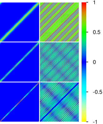
Figure S2: Color plots of certain symmetric eigenstates $\psi(x_{1},x_{2})$ of the 1D Hamiltonian for $U=1$ and $N=128$ in $x_{1}$-$x_{2}$ plane. Top panels correspond to two states in the sector $p_{+}=0$ of total momentum with relative level number (of this sector and with states ordered by increasing energies) being $l=64$ (left) and $l=44$ (right). Center panels correspond to $p_{+}=21\pi/32\approx 2\pi/3$ with $l=64$ (left) and $l=43$ (right). Bottom panels correspond to $p_{+}=63\pi/64\approx\pi$ with $l=62$ (left) and $l=43$ (right).

In Fig. S2 we show some examples of 1D eigenstates of the quantum Hamiltonian (1) obtained from (the real or imaginary part of) Eq. (S9) as explained in the last section from symmetrized block eigenstates (with $65$ or $64$ levels per symmetrized $p_{+}$ sector). The parameters are $U=1$, $N=128$ and three values of $k=p_{+}=0$, $p_{+}\approx 2\pi/3$ and $p_{+}\approx\pi$. For states with (near) maximal energy (for their respective $p_{+}$ sector) one sees a strong localization on the diagonal indicating a strong localization in the relative coordinate $\Delta x$. For relative level numbers close to $2/3$ of the maximal level number the states extend to the full space except for $p_{+}\approx\pi$ where a small strip close to the diagonal is excluded. This is a clear effect of energy miss-match and the very strong interaction on the diagonal if compared to the strongly reduced kinetic energy. The (presence or absence of) change of colors in the center of mass direction indicate the periodic oscillations due the wave number $p_{+}$ in this direction.

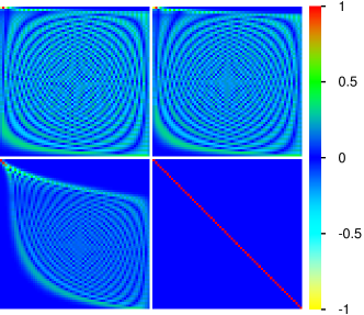
Figure S3: Schematic representation of all symmetric block eigenstates for the 1D case and $U=1$, $N=128$ in relative coordinate $\Delta x$ corresponding to the horizontal axis and with block level number $l$ corresponding to the vertical axis. The different panels correspond to different values of the conserved total momentum which are: $p_{+}=0$ (top left), $p_{+}=21\pi/32\approx 2\pi/3$ (top right), $p_{+}=63\pi/64\approx\pi$ (bottom left) and $p_{+}=\pi$ exactly (bottom right).

Fig. S3 shows a schematic representation of all symmetrized 1D block eigenstates of certain $p_{+}$ sectors (for $U=1$, $N=128$). The horizontal axis of each panel corresponds to $0\leq\Delta x\lesssim N/2$ and the vertical axis to the level number $0\leq l\lesssim 64$ (bottom/top for lowest/largest sector energies) of the shown $p_{+}$ sectors. For $p_{+}=0$ and $p_{+}\approx 2\pi/3$ there is at top energies a very small number of states with rather strong localization at $\Delta x$ close to 0 (values $\Delta x$ close to $N$ are not visible due to the symmetrization). Then there is a big majority of states which are completely delocalized on the full $\Delta x$ interval with certain wavelength values depending on the level number. At lowest energies there is also a very small number of states with significant localization close at $\Delta x\approx N/2$ which is the minimum of the 1D interaction potential. For $p_{+}\approx\pi$ but different from $\pi$ the top (bottom) energy ranges of strong localization at $\Delta x\approx 0$ ($\Delta x\approx N/2$) are strongly enhanced and the intermediate “delocalized” states are quite strongly excluded from small $\Delta x$ values due to an energy miss-match caused by the very strong relative interaction (if compared to the reduced kinetic energy). At $p_{+}=\pi$ exactly there is perfect localization at single $\Delta x$ sites for each state since in this case the kinetic energy vanishes exactly and the corresponding block Hamiltonian is already diagonal with eigenvalues given by the interaction values $U(\Delta x)$.

These observations of Fig. S3 explain quite clearly the behavior of the time evolution of the wave function in block representation visible in the bottom panels of Fig. 1. For sectors with $p_{+}\approx\pi$ an initial block state localized at $\Delta x=1$ will have only contributions from the strongly localized block eigenstates at top energies while other extended block eigenstates have nearly no amplitude at small $\Delta x$ and do not contribute in the initial state (when the latter is expanded in terms of block eigenstates). Therefore there is nearly perfect localization for these sectors (with $p_{+}\approx\pi$) also for long times. For other values of $p_{+}$ quite different from $\pi$ the number of localized top energy states is reduced. However, they still produce an enhanced contribution in the eigenvector expansion of the initial state. Now (most of) the other extended block eigenstates are not excluded/forbidden at small $\Delta x$ values and they have also a certain contribution in the eigenvector expansion, but still with smaller coefficients than the localized top energy states. Therefore in the time evolution a quite significant fraction of probability stays localized while the complementary fraction of density propagates through the whole system.

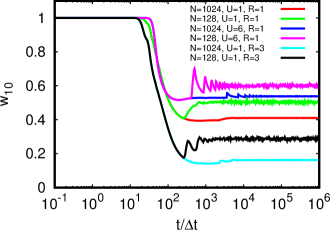
Figure S4: Time dependence of the quantum probability $w_{10}$ to find both particles in the relative strip $\Delta\bar{x}\leq 10$ for the exact 1D time evolution for different values of the parameters $N$, $U$ and $R$ with an initial symmetrized state where both particles are localized (at $x_{1}\approx x_{2}\approx N/2$) at distance $\Delta\bar{x}=R$.

To characterize the quantum probability to form compact electron pairs we compute (for the 1D case) the following quantity:

$$w_{10}=\sum_{x_{1}=0}^{N-1}\sum_{\Delta x=-10}^{10}|\psi(x_{1},x_{1}+\Delta x)|^{2}$$ (S12)

where the sum $x_{1}+\Delta x$ is taken modulo $N$ and $\psi(x_{1},x_{2})$ represents the wave function (in position representation) of the quantum state for which we want to compute $w_{10}$, typically a state obtained from the exact 1D quantum time evolution. This quantity is just the quantum probability to find both particles in the relative strip $\Delta\bar{x}\leq 10$. One can also compute $w_{10}$ from the wave function $\bar{\psi}(k,\Delta x)$ in block representation by sums over all $k$ values and $\Delta x$ values such that either $\Delta x\leq 10$ or $\Delta x\geq N-10$.

Fig. S4 shows the time dependence of $w_{10}$ using the same (type of) time evolution data used for Fig. 1 for different parameter combinations with $N=128,1024$, $U=1,6$ for $R=1$ or $U=1$ for $R=3$ (here $R$ is the initial distance of the particles). We see in all cases that $w_{10}$ saturates at long times at a finite value which is significantly above its ergodic values $w_{\rm erg.}=21/N$ (maybe except for $N=128$, $U=1$ and $R=3$) assuming a perfectly uniform wave function amplitude. Increasing $R=1$ to $R=3$ clearly reduces the pair formation probability while increasing the interaction from $U=1$ to $U=6$ increases the value of $w_{10}$. For the data at $N=128$ there is also a considerable finite size effect.

Appendix E S4. Additional data for the 2D quantum case

Before presenting some additional data for the 2D quantum case, we provide here explicit formulas for the quantities shown in Figs. 4, 5. Assuming that $\psi(x_{1},y_{1},x_{2},y_{2})$ is the wave function in position space obtained from the Totter formula 2D time evolution top panels of Fig. 4 show the density in $\Delta x$-$\Delta y$ plane obtained from:

$$\rho_{\rm rel}(\Delta x,\Delta y)=\sum_{x_{1},x_{2}}|\psi(x_{1},y_{1},x_{1}+\Delta x,y_{1}+\Delta y)|^{2}$$ (S13)

(with position sums taken modulo $N$) and bottom panels show the density in $x_{1}$-$x_{2}$ plane obtained from:

$$\rho_{XX}(x_{1},x_{2})=\sum_{y_{1},y_{2}}|\psi(x_{1},y_{1},x_{2},y_{2})|^{2}\ .$$ (S14)

The quantum probability $w_{\Delta R}$ to find both electrons at $\Delta\bar{x}\leq\Delta R$ and $\Delta\bar{y}\leq\Delta R$ is computed from:

$$w_{\Delta R}=\sum_{\Delta\bar{x}\leq\Delta R,\Delta\bar{y}\leq\Delta R}\rho_{\rm rel}(\Delta x,\Delta y)$$ (S15)

(with $\Delta\bar{x}=\min(\Delta x,N-\Delta x)$ and similarly for $\Delta y$). For the case of exact 2D block time evolution $w_{\Delta R}$ is computed as in (S15) but with $\rho_{\rm rel}(\Delta x,\Delta y)$ replaced by $|\bar{\psi}(p_{+x},p_{+y},\Delta x,\Delta y)|^{2}$ (at certain given values of $p_{+x},p_{+y}$). Here we mostly use the quantity $w_{10}$ corresponding to $\Delta R=10$ but below we also show some data for $w_{2}$ corresponding to $\Delta R=2$.

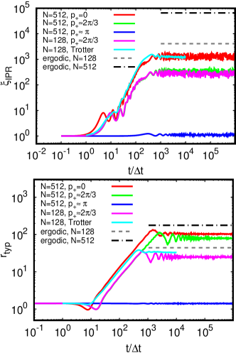
Figure S5: Time dependence of the inverse participation ratio $\xi_{\rm IPR}$ (see Eq. (S16); top panel) and typical distance $r_{\rm typ}$ (see Eq. (S17); bottom panel) computed from the density in $\Delta x$-$\Delta y$ plane for the same cases and raw data of Fig. 4. The dashed grey (dashed-dotted black) line shows the ergodic value for $N=128$ ($N=512$) assuming a uniform density in $\Delta x$-$\Delta y$ plane given by $\xi_{\rm IPR,erg}=(N/2)^{2}$ and $r_{\rm typ,erg}=0.692\times(N/2)$.

In Fig. S5, we show for the same cases and raw data (same 2D time evolution wave functions) used for Fig. 4 the time dependence of the inverse participation ratio defined by:

$$\xi_{\rm IPR}=\left(\sum_{\Delta x,\Delta y}\rho_{\rm rel,sym}^{2}(\Delta x,\Delta y)\right)^{-1}$$ (S16)

($\rho_{\rm rel,sym}$ is the symmetrized density with respect to the two symmetries $\Delta x\leftrightarrow N-\Delta x$ and $\Delta y\leftrightarrow N-\Delta y$ obtained from $\rho_{\rm rel}$) and the typical particle distance:

$$r_{\rm typ}=\exp[\langle\ln(\sqrt{\Delta\bar{x}^{2}+\Delta\bar{y}^{2}}+1)\rangle]-1$$ (S17)

where the average $\langle\cdots\rangle$ is done with respect to the symmetrized density $\rho_{\rm rel,sym}$.

The inverse participation ratio provides roughly the number of sites over which $\rho_{\rm rel,sym}(\Delta x,\Delta y)$ is mostly concentrated or localized. The saturation values at long times well below the ergodic value clearly indicate a considerable pair formation probability confirming the findings of Fig. 5. For $p_{+}\approx\pi$ (case of near perfect localization) one can see values slightly above unity ($\xi_{\rm IPR}\lesssim 1.2$) for all time scales. Note that for this case $w_{10}$ shown in Fig. 5 takes the value 1 with numerical precision (error below $10^{-14}$).

The other quantity $r_{\rm typ}$ is mostly dominated by the fraction of density associated to free electron propagation. Therefore the ratio $r_{\rm typ}/r_{\rm typ,erg}$ corresponds to the complementary non-pair formation probability and indeed the quantity $1-r_{\rm typ}/r_{\rm typ,erg}$ behaves qualitatively similarly as $w_{10}$. For the case of near perfect localization at $p_{+}\approx\pi$ we have for all time scales $r_{\rm typ}\approx\sqrt{2}$ (corresponding to $\Delta x=\Delta y=1$) with some slight fluctuations $\pm 0.02$ at long times.

Globally, we believe that $w_{10}$ is more useful and suitable than $\xi_{\rm IPR}$ or $r_{\rm typ}$ to describe the pair formation probability which is the reason why we have chosen to show in the main part of this work the time dependence of $w_{\rm 10}$ in Fig. 4.

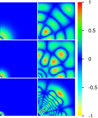
Figure S6: Certain 2D (totally symmetrized) block eigenstates in $\Delta x$-$\Delta y$ plane for $U=2$, $N=128$. Top panels correspond to conserved total momentum $p_{+}=p_{+x}=p_{+y}=0$ and block level numbers $l=2143$ (left) and $l=2135$ (right). Center panels correspond to $p_{+}=21\pi/32\approx 2\pi/3$, $l=2143$ (left), $l=2131$ (right). Bottom panels correspond to $p_{+}=63\pi/64\approx\pi$, $l=2072$ (left), $l=1991$ (right).

Some examples of localized and delocalized 2D block eigenfunctions for the three sectors $p_{+}=p_{+x}=p_{+y}=0$, $p_{+}\approx 2\pi/3$ and $p_{+}\approx\pi$ and $N=128$, $U=2$ are presented in Fig. S6. As in 1D top energy eigenstates (with respect to their $p_{+}$ sector) are localized at $\Delta x\approx\Delta y\approx 0$ and lower energy eigenstates are delocalized. For $p_{+}=0$ and $p_{+}\approx 2\pi/3$ the number of localized states is very small and already at sector level numbers slightly below their maximal value delocalization sets in. For $p_{+}\approx\pi$ the number of localized states is larger and for the delocalized states the zone close to $\Delta x\approx\Delta y\approx 0$ is forbidden such that these states do not contribute in the time evolution if the initial state is localized at $\Delta x=\Delta y=R$ for some small value of $R=1$ or $R=3$. These findings are very similar to the 1D case (see above discussion of Figs. S3,S4) and help to understand the 2D time evolution results shown in Figs. 3-5.

One can also see, especially for the delocalized eigenstates, a spatial node structure indicating a rough and very approximate angular momentum conservation. However, this is not exact due to the square form of available space, discrete lattice structure and also the cosinus 2D band form of kinetic energy (for the relative coordinates). Furthermore, our limitation to totally symmetrized block eigenstates (with respect to the discrete symmetries explained in Sec. S2) plays a role here.

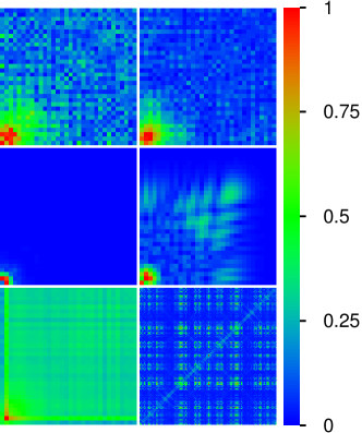
Figure S7: Certain wave function densities for different cases of the 2D time evolution and weak interaction $U=0.5$. Top and center panels correspond to the same type of quantity as shown in Fig. 3 with $p_{+}=p_{+x}=p_{+y}=0$ (top left), $p_{+}=85\pi/128\approx 2\pi/3$ (top right), $p_{+}=255\pi/256\approx\pi$ (center left), all three for $N=512$ and $t=10^{5}\,\Delta t$, and $p_{+}=63\pi/64\approx\pi$, $N=128$, $t=3090\,\Delta t$ (center right). Bottom panels correspond to the Trotter formula approximation for $N=128$ and $t=9487\,\Delta t$ with left panel showing the density in relative coordinates obtained from a sum over $x_{1}$ and $y_{1}$ and with right panel showing the density in $x_{1}$-$x_{2}$ plane obtained from a sum over $y_{1}$ and $y_{2}$. All panels (except bottom right) show to a zoomed region $0\leq\Delta x,\Delta y<32$ in $\Delta x$-$\Delta y$ plane. At ourwebpage videos corresponding to the cases of all panels of this figure (and also for $N=128$ with $p_{+}=0$ and $p_{+}=21\pi/32\approx 2\pi/3$) are provided.

The 2D pair formation effect still exists at the smaller interaction value $U=0.5$ even though it is less pronounced as can be seen in Fig. S7 showing certain wave function densities obtained from both types of 2D time evolution methods. For $N=128$ the Trotter formula results indicate the formation of a very slight diagonal in the density $\rho_{XX}(x_{1},x_{2})$ and a modest localization effect in $\rho_{\rm rel}(\Delta x,\Delta y)$. However, here the density weight corresponding to free electron propagation is quite high. For $N=128$ this is also confirmed by the 2D block time evolution results (not shown in Fig. S7 except for one special case) but for $N=512$ the density related to free propagation is quite strongly reduced in comparison to $N=128$. As can be seen in both top and left center panels of Fig. S7 for $N=512$ there is a considerable density for the compact electron pair. However, for $p_{+}=0$ ($p_{+}\approx 2\pi/3$) one still clearly see a quite strong (quite modest) density related to free propagation while for $p_{+}\approx\pi$ the latter is absent. The right center panel shows the case $N=128$ and $p_{+}\approx\pi$ (strong localization case at $N=512$) at a certain intermediate time when one can briefly see a density related to free propagation which is however smeared out at longer times.

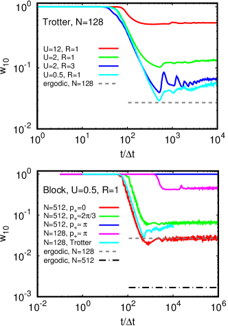
Figure S8: Time dependence of the quantum probability $w_{10}$ to find both particles in the relative square $\Delta\bar{x}\leq 10$, $\Delta\bar{y}\leq 10$. Top panel corresponds to the full space 2D time evolution using the Trotter formula approximation for $N=128$ and different values of $U$ and initial particle distance $R$. Bottom panel corresponds to $U=0.5$, $R=1$ and compares certain cases of the exact 2D block time evolution in certain sectors of conserved momenta $p_{+}=p_{+x}=p_{+y}$ with the result obtained from the Trotter formula approximation. The precise values of $p_{+}$ are : $p_{+}=0$, $p_{+}=85\pi/128\approx 2\pi/3$, $p_{+}=255\pi/256\approx\pi$ all three for $N=512$ and $p_{+}=63\pi/64\approx\pi$ for $N=128$. The top blue line has at $t=10^{6}$ a numerical of $0.99918$. In both panels the grey dashed horizontal line corresponds to the value of $w_{\rm erg.}=(21/128)^{2}\approx 0.0269$ assuming a constant (ergodic) density on a square of size $N=128$. In bottom panel the black dashed-dotted horizontal line corresponds to the value of $w_{\rm erg.}=(21/512)^{2}\approx 0.00168$ assuming a constant density on a square of size $N=512$.

The qualitative findings of Fig. S7 for $U=0.5$ are confirmed by the time dependence of $w_{10}$ shown in the lower panel of Fig. S8 for the cases of Fig. S7. For $N=512$ and $p_{+}=0$ or $p_{+}\approx 2\pi/3$ the saturation values of $w_{10}$ are below 0.1 but still significantly above the ergodic value. For $p_{+}\approx\pi$ and $N=512$ the saturation value $w_{10}=0.99988$ is nearly maximal while for $N=128$ it is lower but still quite elevated, $w_{10}\approx 0.45$, showing a certain finite size effect for this case. The saturation of the Trotter formula case at $N=128$ is $w_{10}\approx 0.05$ which is rather low but still roughly twice the ergodic value which is $0.027$.

The top panel of Fig. S7 shows the time dependence of $w_{10}$ for the Trotter formula case and other parameter values $U=0.5,\,2,\,12$ at $R=1$ and $U=2$ at $R=3$ with $R$ being the initial value of $\Delta\bar{x}=\Delta\bar{y}$. As in 1D (see Fig. S4) stronger (lower) interaction increases (reduces) the pair formation probability and when $R$ is increased the pair formation probability is reduced.

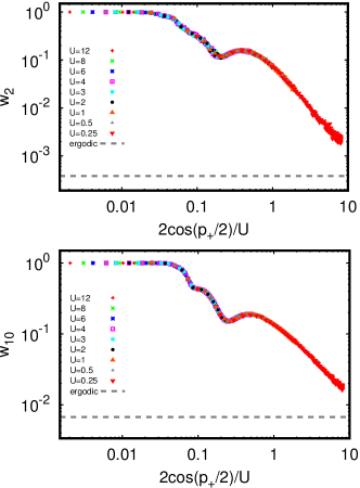
Figure S9: Dependence of $w_{\Delta R}$ with $\Delta R=2$ ($\Delta R=10$) in top (bottom) panel to find both particles in the relative square $\Delta\bar{x}\leq\Delta R$ on the scaling parameter $2\cos(p_{+}/2)/U$ for different interaction values $0.25\leq U\leq 12$, $N=256$ and $p_{+}=p_{+x}=p_{+y}\in[0,\pi]$. The dashed gray line corresponds to the ergodic probability $w_{\rm erg.}=((2\Delta R+1)/256)^{2}$ assuming a constant density on a square of size $N=256$. The value of $w_{\Delta R}$ has been computed from the exact 2D time evolution in different $p_{+}$ sectors using a time average over 21 time values $t$ with logarithmic density such $10^{4}\leq t/\Delta t\leq 10^{6}$.

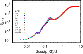
Figure S10: Dependence of the 2D inverse participation ratio $\xi_{\rm IPR}$ in symmetrized $\Delta x$-$\Delta y$ plane on the scaling parameter $2\cos(p_{+}/2)/U$. The dashed grey line corresponds to the ergodic value $\xi_{\rm IPR,erg.}=(N/2)^{2}\approx 1.6\times 10^{4}$ assuming a uniform distribution on a square of size $N/2=128$ (due to symmetrization). $\xi_{\rm IPR}$ has been computed from the same raw data (time dependent wave functions), using the same parameters and same time average as in Fig. S9.

In Fig. S9 we show for $N=256$ the dependence of the saturation value of $w_{\Delta R}$ for $\Delta R=2$ (top panel) and $\Delta R=10$ (bottom panel), computed as the average over 21 time values $t$ with $10^{4}\leq t/\Delta t\leq 10^{6}$, on the scaling parameter $C=2\cos(p_{+}/2)/U$ (here we only consider $0\leq p_{+}\leq\pi$ such that $C\geq 0$). This parameter is the ratio of the hopping matrix element and the interaction amplitude of the effective 2D one-particle tight binding model of the block at $p_{+}=p_{+x}=p_{+y}$ (see Sec. S2 for details). We have also computed the same scaling curves for $N=512$ with a reduced density of data points. These curves are identical to (slightly below) the case $N=256$ for $C\lesssim 2$ ($C\gtrsim 2$) with a rough factor of 0.5 at $C=8$.

The scaling dependence is quite obvious and clearly confirms the role of the total conserved momentum $p_{+}$ for the kinetic energy amplitude of the relative coordinates. At small values of $C\ll 1$ we have perfect localization (perfect pair formation) with $w_{2}\approx w_{10}\approx 1$ and then the curves decrease down to a modest local minimum at $C\approx 0.2$ which is followed by a local maximum at $C\approx 0.3$. Then they continue to decrease down to the value of $2.2\times 10^{-3}$ ($1.8\times 10^{-2}$) for $w_{2}$ ($w_{10}$) at $C=8$. These minimal values are still clearly above the ergodic values $3.8\times 10^{-4}$ ($6.7\times 10^{-3}$).

Fig. S10 shows the same type of scaling curve but for the inverse participation ratio $\xi_{\rm IPR}$ which has a value of $\approx 1$ for $C\ll 1$ for the case of perfect localization (perfect pair formation). Then the curve increases up to a modest local maximum at $C\approx 0.2$ followed by a local minimum at $C\approx 0.3$. After this it continues to increase until it saturates for $C\gtrsim 3$ at the value $\xi_{\rm IPR}\approx 6.9\times 10^{3}$ which is clearly below the ergodic value $1.6\times 10^{4}$.

Appendix F S5. Videos of TIP time evolution in 2D

Two videos of the 2D time evolution for the cases of (i) Fig. 3 (videoforfig3.avi), top right panel (exact 2D block time evolution of sector $p_{+}=21\pi/32\approx 2\pi/3$) and (ii) Fig. 4 (videoforfig4.avi), bottom panels (density in $x_{1}$-$x_{2}$ plane obtained from the Trotter formula 2D time evolution) are provided. For (i) the video is composed of 702 images (25 images per second of video) at time values $t_{0}=0$ and $t_{i}=\Delta t\times 10^{(i-101)/100}$ for $1\leq i\leq 701$ (with $\Delta t=1/B_{2}=1/(16+U)$) corresponding to a logarithmic time scale in the range $\Delta t\times 10^{-1}\leq t\leq\Delta t\times 10^{6}$. For (ii) the video is composed of 464 images at integer multiples of $t_{i}=l_{i}\Delta t$ with $l_{i}=i$ for $0\leq i\leq 87$ and roughly $l_{i+1}\approx 10^{1/100}\,l_{i}$ for $87\leq i<463$ (such that $l_{463}=10^{4}$) corresponding roughly to a logarithmic (linear) time scale for $t/\Delta t>87$ ($t/\Delta t\leq 87$) in the range $\Delta t\leq t\leq\Delta t\times 10^{4}$.

At our web page ourwebpage http://www.quantware.ups-tlse.fr/QWLIB/coulombelectronpairs further videos corresponding to the panels of Fig. 1 (exact full space 1D time evolution), Fig. S7 (both cases of 2D time evolution for $U=0.5$), and other panels of Figs. 3,4 are available. The time scales are always as in the cases (i) (exact 1D, with modified $\Delta t=1/B_{1}=1/(8+U)$, or block 2D time evolution) or (ii) (Trotter formula 2D time evolution).

References

- (1) M.C. Gutzwiller, Effect of correlation on the ferromagnetism of transition metals, Phys. Rev. Lett. 10, 159 (1963).
- (2) J. Hubbard, Electron correlations in narrow energy bands, Proc. R. Soc. Lond. A 276, 238 (1963).
- (3) M.C. Gutzwiller, Correlation of electrons in a narrow s band, Phys. Rev. 137 A1726 (1965).
- (4) Y. Cao, V. Fatemi, S. Fang, K. Watanabe, T. Taniguchi, E. Kaxiras and P. Jarillo-Herrero, Unconventional superconductivity in magic-angle graphene superlattices, Nature 556, 43 (2018).
- (5) Y. Cao, V. Fatemi, A. Demir, S. Fang, S.L. Tomarken, J.Y. Luo, J.D. Sanchez-Yamagishi, K. Watanabe, T. Taniguchi, E. Kaxiras, R.C. Ashoori and P. Jarillo-Herrero, Correlated insulator behaviour at half-filling in magic-angle graphene superlattices, Nature 556, 80 (2018).
- (6) X. Lu, P. Stepanov, W. Yang, M. Xie, M.A. Aamir, I. Das, C. Urgell, K. Watanabe, T. Taniguchi, G. Zhang, A. Bachtold, A.H. MacDonald and D.K. Efetov, Superconductors, orbital magnets, and correlated states in magic angle bilayer graphene, Nature 574, 653 (2019).
- (7) P. Stepanov, I. Das, X. Lu, A. Fahimniya, K. Watanabe, T. Taniguchi, F.H.L. Koppens, K. Lischner, L. Levitov and D.K. Efetov, The interplay of insulating and superconducting orders in magic-angle graphene bilayers, arXiv:1911.09198 [cond-mat.supr-con] (2019).
- (8) M. Koshino, N.F.Q. Yuan, T. Koretsune, M. Ochi, K. Kuroki, and L. Fu, Maximally localized Wannier orbitals and the extended Hubbard model for twisted bilayer graphene, Phys. Rev. X 8, 031087 (2018).
- (9) N.F.Q. Yuan and L. Fu, Model for the metal-insulator transition in graphene superlattices and beyond, Phys. Rev. B 98, 045103 (2018).
- (10) J. Kang and O. Vafek, Symmetry, maximally localized Wannier states, and a low-energy model for twisted bilayer graphene narrow bands, Phys. Rev. X 8, 031088 (2018).
- (11) X. Wu, W. Hanke, M. Fink, M. Klett and R. Thomale, Harmonic fingerprint of unconventional superconductivity in twisted bilayer graphene, arXiv:1909.03514 [cond-mat.supr-con] (2019).
- (12) R. Bistrizer and A.H. MacDonald, Moire bands in twisted double-layer graphene, Proc. Nat. Acad. Sci. 108, 12233 (2011).
- (13) M.I.B. Utama, R.J. Koch, K. Lee, N. Leconte, H. Li, S. Zhao, L. Jiang, J. Zhu, K. Watanabe, T. Taniguchi, P.D. Ashby, A.Weber-Bargioni, A. Zettl, C. Jozwiak, J. Jung, E. Rotenberg, A. Bostwick and F. Wang, Visualization of the flat electronic band in twisted bilayer graphene near the magic angle twist, arXiv:1912.00587 [cond-mat.mes-hall] (2019).
- (14) See Supplemental Material at http:XXXX that contains: i) mathematical details on the numerical diagonalization and quantum time evolution methods exploiting the conserved total momentum, ii) extra-figures and videos that support the main conclusions and results.
- (15) K.M. Frahm and D.L.Shepelyansky, Available: http://www.quantware.ups-tlse.fr/QWLIB/coulombelectronpairs/; Accessed January (2020).
- (16) S.-J. Chang and K.-J. Shi, Evolution and exact eigenstates of a resonant quantum system, Phys. Rev. A 34, 7 (1986).
- (17) K.M. Frahm, R. Fleckinger and D.L. Shepelyansky, Quantum chaos and random matrix theory for fidelity decay in quantum computations with static imperfections, Eur. Phys. J. D 29, 139 (2004).
- (18) K.M. Frahm and D.L.Shepelyansky, Delocalization of two interacting particles in the 2D Harper model, Eur. Phys. J. B 89, 8 (2016).