Pulse-qubit interaction in a superconducting circuit under frictively dissipative environment

Abstract

Microwave pulses are used ubiquitously to control and measure qubits fabricated on superconducting circuits. Due to continual environmental coupling, the qubits undergo decoherence both when it is free and during its interaction with the microwave pulse. As quantum logic gates are executed through pulse-qubit interaction, we study theoretically the decoherence-induced effects during the interaction, especially the variations of the pulse, under a dissipative environment with linear spectral distribution. We find that a transmissible pulse of finite width adopts an asymmetric multi-hump shape, due to the imbalanced pumping and emitting rates of the qubit during inversion when the environment is present. The pulse shape reduces to a solitonic pulse at vanishing dissipation and a pulse train at strong dissipation. We give detailed analysis of the environmental origin from both the perspectives of envelope and phase of the propagating pulse.

I Introduction

Superconducting qubit circuits have become a major platform for testing quantum computation protocols (clarke08, ) and quantum optical effects (jqyou11, ; ian10, ). As a solid-state device fabricated on semiconductor substrates, a superconducting circuit suffers from noises originated from multiple sources such as the underlying dielectric (martinis05, ) and the bias input (martinis03, ), most notably in form of $1/f$ noise (bialczak07, ; yoshihara06, ). The noises induce decoherences, in terms of both transverse dephasing and longitudinal relaxations, in the qubits (ithier05, ). Hence, succesful demonstrations of optical effects and computational operation, such as state readouts, often become contests against the decoherence times (mallet09, ). A quantitative understanding of decoherence (yu17, ) becomes, therefore, essential in the further development of superconducting circuits.

Throughout the years, multiple studies have been devoted to the descriptions of decoherences on this solid-state system (tian02, ; jqyou07, ; mcdermott09, ). In particular, Ref. (tian02, ) models a SQUID loop induced decoherence during readout, based on a noise spectrum framed on the Leggett model of infinitesimally-spaced linear resonators(caldeira83, ; leggett84, ). Ref. (jqyou07, ) estimates the relaxation of a standalone qubit directly from Fermi golden rules. Few studies actually consider the decoherence induced on a superconducting qubit during its interaction with a microwave pulse. A correct modeling of the decoherence induced during the course of interaction would benefit the designs of entanglement operations (wei06, ; neeley10, ) and projective measurements (mallet09, ) on qubits, which are carried out through coupling them with definite types of microwave pulses.

Since a resonant pulse forms time-dependent dressed states with the qubit, which give rise to different decay channels than those of the qubit bare states. the qubit relaxations are highly dependent on the variations of the envelope and phase of the traveling microwave pulse. Inversely, the change incurred on the envelope and phase after the pulse propagates through the qubit are highly dependent on the decoherence of the qubit, which are often ignored in the studies related to resonant pulses. Here, we use an adiabatic master equation to register the environmental influence on the qubit during the course of interaction and compute how a given dissipative environment would affect the output pulse in both its envelope and phase after it is applied to the qubit.

In line with superconducting circuit systems, which contain the qubits that are made up by Josephson junction barriers (martinis05, ), the environment is assumed to be frictive (caldeira81, ), where the barriers are considered Ohmic interfaces. In other words, its spectral density $J(\omega)$ is assumed linear in its frequency dependence (widom82, ). Under such an assumption, we find that resonant pulses behave differently during their propagation through the qubit, depending on the linear scale factor embodied in the spectrum density. Modeling the qubit evolution through a microscopic master equation and the pulse travel through Maxwell equations, we obtain the limiting solution for a vanishing scale factor to be a solitonic pulse, which adopts a symmetric hump shape. When the scale factor becomes large to represent a strong dissipative environment, the solution approaches another asymptotic limit that associates with a continuous pulse train.

Between these two limits, solutions to the coupled model equations admit pulse envelope shapes with multiple humps of various heights and monotonic increase in phase with various rates, all of which depend on the magnitude of dissipation. Pulses are only admissible with multiple peaks because the qubit and the environment are of competing nature in the absorption and the re-emission of microwave pulses. We analyze quantitatively how the enveloped pulse area is determined by this competing nature in Sec. III. The analysis is based on the solution to the coupled Maxwell-master equations derived from an adiabatic pulse-qubit interation model we explain in Sec. II. We also analyze the variation of the pulse phase in Sec. IV before presenting the conclusions in Sec. V.

II Pulse-qubit interaction

The interacting system of a qubit and an incident pulse is described by the time-dependent Hamiltonian ($\hbar=1$)

$$H_{S}(t)=\frac{\omega_{z}}{2}\sigma_{z}-\mu E(t)(\sigma_{+}+\sigma_{-})$$ (1)

in the Schroedinger picture, where the Pauli matrices associates with the free energy and the transitions of the qubit and $E(t)=\mathcal{E}(t)\cos(\varphi-kx+\omega t)$ describes the electric field part of the dipole-field interaction Hamiltonian. $\mu$ is the qubit dipole moment. For a resonant pulse, the dressed states that diagonalize the Hamiltonian are

$$\left|\varepsilon_{\pm}(t)\right\rangle=\text{$\frac{1}{\sqrt{2}}\left[e^{-i\alpha(t)}\left|e\right\rangle\mp\left|g\right\rangle\right]$}$$ (2)

where we have let $+$ ($-$) sign associate with the upper (lower) energy state and $\alpha(t)=\varphi(t)-kx$ designate a time-dependent phase factor. Correspondingly, we define $\nu_{-}=\left|\varepsilon_{-}\right\rangle\left\langle\varepsilon_{+}\right|$ and it Hermitian conjugate $\nu_{+}$ as an annhilation and creation operator pair for the dressed states with eigenenergies $\Omega$ and $-\Omega$, respectively, where $\Omega(t)=\mu\mathcal{E}(t)$.

The bath is customarily written as a multimode resonator $H_{B}=\sum_{j}\omega_{j}\left(a_{j}^{\dagger}a_{j}\right)$, from which the qubit-bath coupling is expressed by the Hamiltonian

$$H_{I}=\sum_{j}g_{j}\left(\left|e\right\rangle\left\langle g\right|+\left|g\right\rangle\left\langle e\right|\right)\left(a_{j}^{\dagger}+a_{j}\right).$$ (3)

During the propagation of the microwave pulse, the qubit operators in $H_{I}$ become the dressed operators associated with the basis vectors of Eq. (2) and $H_{I}$ is correspondingly transformed to $H_{I}(t)$ under the moving reference frame of the pulse. In this frame, the total system-bath evolution under the interaction picture is described by the Liouville equation

$$\frac{d\rho(t)}{dt}=-i\left[H_{I}(t),\rho(t)\right]$$ (4)

for the density matrix $\rho=\rho_{\mathrm{S}}\otimes w$ of the density, i.e. $\rho_{S}$ is the density matrix of the dressed qubit while $w$ is the density matrix of the environment. Under typical considerations, the environment is regarded as a reservoir with infinite energy supply so it remains at a static density distribution $w$ during the course of interaction while the environmental feedback affects the density distribution of the system such that $\rho_{\mathrm{S}}=\rho_{\mathrm{S}}(t)$. Henceforth, substituting the tensor product of density matrices into Eq. (4) and tracing out the bath space, one arrives at the master equation (ian18, )

$$\frac{d\rho_{\mathrm{S}}(t)}{dt}=-i\left[H_{\mathrm{S}},\rho_{\mathrm{S}}\right]+\gamma\sin^{2}(\varphi-kx)\biggl{\{}\nu_{-}\rho_{\mathrm{S}}\nu_{+}\\ -\frac{1}{2}\left(\nu_{+}\nu_{-}\rho_{\mathrm{S}}+\rho_{\mathrm{S}}\nu_{+}\nu_{-}\right)\biggr{\}}$$ (5)

where $\gamma(\Omega)=2\pi\sum_{j}g_{j}^{2}\delta(\omega_{j}-\Omega)$ represents the net decay rate stemmed from the bath spectral distribution.

The propagating microwave pulse is described by the Maxwell equation

$$\frac{\partial^{2}E}{\partial t^{2}}-c^{2}\frac{\partial^{2}E}{\partial x^{2}}=-\frac{1}{\epsilon_{0}}\frac{\partial^{2}P}{\partial t^{2}}$$ (6)

where $P(t)=\left[\mathcal{P}(t)\exp i\{\varphi(t)+\omega t-kx\}+\mathrm{c.c.}\right]/2$ represents the macroscopic polarization of the qubit as a dipole. We assume the same phase $\varphi(t)$ to ignore the calculation of the dispersive effects and the complex amplitude correlates with the density matrix through $\mathcal{P}=\mathrm{tr}\{\mu\sigma_{x}\rho_{\mathrm{S}}\}$.

III Propagation under dissipation

III.1 The area equation

In order to make the master-Maxwell equation pair (5)-(6) solvable through decoupling, Eq. (6) is customarily first reduced to first-order equations in the coordinate of local time $\tau=t-x/v$

$$\frac{d\mathcal{E}}{d\tau} =\frac{\omega}{2(1-c/v)\epsilon_{0}}\Im\{\mathcal{P}\},$$ (7)

$$\frac{d\varphi}{d\tau} =-\frac{\omega}{2(1-c/v)\epsilon_{0}\mathcal{E}}\Re\{\mathcal{P}\},$$ (8)

where the differential operator $\partial/\partial\tau$ contracts from $\partial/\partial t+c\partial/\partial x$ up to a proportion constant $(1-c/v)$. The reduction is made possible by assuming the slow-varying envelope approximation, i.e. $\partial\mathcal{E}/\partial t\ll\omega\mathcal{E}$, $\partial\mathcal{E}/\partial x\ll k\mathcal{E}$, etc., which omits the second-order fast-varying terms. The local time $\tau$, which is equivalent to the diagonal axis in the $xt$-plane, can also be regarded as a time mark registered on the wavefront of the pulse.

We have shown in Ref. (ian18, ) that the mixed qubit-field system whose evolution is governed by Eq. (5) under the dressed basis $\left|\varepsilon_{\pm}\right\rangle$ can be solved by perturbative expansion, giving rise to $\mathcal{P}=\mu\left(1-e^{-\Gamma}-i\sin\theta e^{-\Gamma/2}\right)$ for an inital ground-state qubit, where

$$\Gamma(\tau)=\int_{\tau_{0}}^{\tau}ds\,\gamma(\Omega)\sin^{2}(\varphi-kx)$$ (9)

denotes a decoherence factor and $\theta(\tau)=\int_{\tau_{0}}^{\tau}ds\,\Omega(s)$ denotes the enveloped area of the pulse up to time $\tau$. With the determination of $\mathcal{P}$, the equation pair (7)-(8) becomes

$$\frac{d\mathcal{E}}{d\tau} =M^{2}\sin\theta e^{-\Gamma/2},$$ (10)

$$\frac{d\varphi}{d\tau} =\frac{M^{2}}{\mu\mathcal{E}}\left(1-e^{-\Gamma}\right),$$ (11)

where $M=\sqrt{\mu^{2}\omega v/2(c-v)\epsilon_{0}}$. Note that in this form, $\Gamma$, $\mathcal{E}$, and $\varphi$ are inter-dependent, making the equation pair insolvable. Especially, the expression of $\Gamma(\tau)$ demonstrates the memory effect of the culminated feedback from the environment to the pulse. On one hand, it is determined by the spectral distribution of the bath through $\gamma(\Omega)$; on the other, it depends on the historic variation of the phase $\varphi$.

To give a realistic estimate of the environmental influence, the Leggett model (caldeira81, ) is assumed, i.e. $\Gamma=\lambda\theta$ by regarding that the influence contributed by the phase through $\sin^{2}(\varphi-kx)$ averages out over the integration in Eq. (9) and the spectrum $\{g_{j}\}$ of the bath has a linear dependence on $\Omega$. $\lambda$ here acts as a scale factor, for which Eq. (10) becomes the second-order equation

$$\ddot{\theta}=M^{2}e^{-\lambda\theta/2}\sin\theta.$$ (12)

When $\lambda$ vanishes, the equation reduces to a typical pendulum equation, for which a hyper-secant solution exists. This signifies a solitary wave can travel absorption-free when encountering a qubit, analogous to the effect of self-induced transparency (SIT) experienced by a traveling light field through an ensemble of two-level atoms (mccall67, ).

The extra factor $e^{-\lambda\theta/2}$ contributed by the environment does not permit an explicit expression of the solution but does allow an implicit solution. First, by transforming the variable from $\tau$ to $\theta$ in Eq. (12), i.e. letting $\ddot{\theta}=\dot{\theta}(d\dot{\theta}/d\theta)=d(\dot{\theta}^{2})/2d\theta$, the equation order is reduced by one. Then formally integrating by parts over $\theta$ and taking the square root leads to the formula

$$\dot{\theta}=M\sqrt{\frac{2-e^{-\lambda\theta/2}(2\cos\theta+\lambda\sin\theta)}{1+\lambda^{2}/4}}.$$ (13)

Since there is an one-one correspondence between $\theta$ and $\tau$ and the expression of $\dot{\theta}$ is differentiable with respect to $\tau$, taking the reciprocal of $d\theta/d\tau$ and integrating both sides with respect to $\theta$ again leads to the inverted function

$$\tau(\theta)=\tau_{0}+\frac{\sqrt{1+\lambda^{2}/4}}{M}\times\\ \int_{\theta_{0}}^{\theta}d\vartheta\left[2-e^{-\lambda\vartheta/2}(2\cos\vartheta+\lambda\sin\vartheta)\right]^{-1/2}$$ (14)

that shows the explicit dependence between $\theta$ and $\tau$, where $\theta_{0}\to 0$ at the limit $\tau_{0}\to-\infty$.

III.2 Dissipation of pulse area

Since the definition of $\tau$ is the time measurement from an apparatus traveling at the wave speed $v$, one can regard the apparatus as originally be placed at the pulse wavefront, where the pulse area underneath the envelope is asymptotically zero. Then Eq. (14) as an implicit solution to the wave equation of Eq. (12) should be intrepreted as expressing the time point read from the apparatus when the underneath area culminates to a certain value $\theta$.

In Fig. 1, we plot the $\tau$-$\theta$ relation depicted in Eq. (14) and graphically invert the two reciprocal variables to make the relation appear intuitive. The plots here and hereafter employ experimentally accessible parameters extracted from current studies on superconducting circuit (eichler12, ; wen18, ; wen19, ): the qubit transition frequency $\omega_{z}/2\pi=5$GHz, the coupling strength $\mu\mathcal{E}/2\pi=636$MHz at the pulse peak, and the characteristic time $M^{-1}=0.5$ns that roughly estimates the pulse width at half maximum. The latter is chosen according to typical solitonic pulse generation, where the width is set to 10 cycles long of a resonant microwave signal.

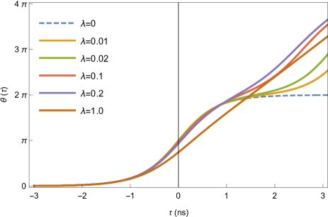
Figure 1: Plot of the enveloped area $\theta(\tau)$ of a microwave pulse during its propagation through a superconducting qubit against local time $\tau$. The dashed curve indicates the scenario of zero decoherence $\lambda=0$: $\theta(\tau)$ converges asymptotically to 0 and $2\pi$ towards the $-\infty$ and the $\infty$ time limits, respectively. The variations of pulse area under the presence of decoherence are given by the different color-coded solid curves (correspondence given in the legend). For example, the red curve indicates the scenario of finite decay with $\lambda=0.1$: $\theta(\tau)$ only converges towards the $-\infty$ end and increases monotonically towards the $\infty$ end. 

We observe that the zero-dissipation curve converges to a horizontal asymptote at $2\pi$, showing that a steady-state solution exists for a solitonic pulse of $2\pi$ enveloping area. The curve is anti-symmetric about $\tau=0$ where $\theta(0)=\pi$. In other words, the time apparatus, which originally travels in front of the incident pulse and has no registered area at $\tau\to-\infty$, has begun to lag into the pulse after it meets the qubit. It has lagged exactly halfway into the pulse at $\tau=0$. For a symmetric-shaped solitonic pulse, this time point coincides with the peak point of the pulse. These observations accord with SIT (mccall67, ), where microwave pulses with initial envelopping area of $2n\pi$ can propagate through the qubit without being absorbed.

Otherwise, with the presence of environmental dissipation, $\tau$ increases monotonically with $\theta$, showing that the longer the pulse sustains its passage through the qubit, the more pulse area is registered by the time apparatus, which is equivalent to energy being extracted by either the qubit or the environment. When the scale factor $\lambda$ remains small, the early development up to $\tau<1$ns remains close to the case of $\lambda=0$. That is, when one regards Eq. (12) as describing a Markovian process, the rate of change of the system at an early stage is determined predominantly by $\sin\theta$, not the environmental $\exp\{-\lambda\theta/2\}$, when $\lambda$ is sufficiently small. During the early interaction, the qubit is being inverted to its excited state and the dissipation described by the Lindbladian in Eq. (5) would make the first half of a $2\pi$-solitonic pulse insufficient to accomplish total inversion at $\tau=0$. The observation is verified when we plot in Fig. 2 the envelope variation against $\tau$ by taking the time derivative of $\theta$ numerically under the same set of scale factors as given in Fig. 1.

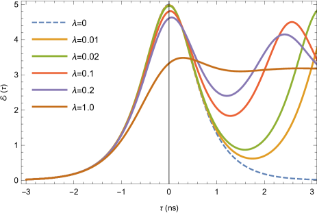
Figure 2: The microwave pulse envelope $\mathcal{E}(\tau)$ as a function of the local time $\tau$ during propagation under environmental dissipation at different scale factor $\lambda$. The dashed curve corresponds to $\lambda=0$ while the solid curves correspond to finite values of $\lambda$, the color coding scheme being identical to that of Fig. 1. The dissipative qubit splits up the envelop in addition to absorbing the microwave photon, whereas the non-dissipative qubit retains the solitonic shape of the pulse. 

Therefore, ever increasing the scale factor $\lambda$ leads the peak point of a solution to Eq. (12) to deviate from $\tau=0$ and leans ever deeper into the right end. The dissipative environment hence breaks the time symmetry of a permissible solution and forces the qubit to fully invert only when $\tau>0$. When $\lambda$ is sufficiently large (e.g. the brown curves in Figs. 1 and 2 with $\lambda=1$), the dissipation becomes so fast that full inversion is never reached. Consequently, apparent deviations from the $\theta=2\pi$ horizontal asymptote occur during the second half of the qubit-pulse interaction. In the fully (respectively, non-fully) inverted case, stimulated (respectively, spontaneous) emission dominates while the qubit flips back to the ground state. Further, if spontaneous emission dominates, $\theta$ follows rather a diagonal asymptote against $\tau$, which corresponds to a leveled horizontal asymptote in $\mathcal{E}(\tau)$. This asymptotic behavior means that when $\exp\{-\lambda\theta/2\}$ dominates $\sin\theta$ in Eq. (12), the admissible solution to Eq. (10) for microwave propagation is a leveled pulse train (i.e. square pulse), which constantly supplies energy to compensate the loss in dissipation and sustain propagation.

In general, since the qubit excitation is already asymmetric about $\tau=0$ (absorbs when $\tau<0$ and emits $\tau>0$) without the dissipation, the dynamic symmetry breaking due to dissipation not only attenuates the obtainable peak registered by the time apparatus, but also unanimously produces $\theta>2\pi$ at the right $\tau\to\infty$ limit. This signifies that a pulse with an initial area less than $2\pi$ cannot fully travel through the qubit and be registered by the time apparatus. The longer the duration of time record, the larger energy should the pulse carry before encountering the qubit.

For the particular cases where $\lambda$ remains small and $\sin\theta$ still dominates, $\theta(\tau)$ can approach a value either greater or less than the diagonal $\theta$-$\tau$ asymptote during the later part of propagation. It depends on the emission rate, which is measured from the combined stimulated and spontaneous emissions into the circuit waveguide, relative to $\lambda$. In addition, if we regard Eq. (12) as expressing the derivative $\dot{\mathcal{E}}$, we find that the extrema of $\mathcal{E}$ given in Fig. 2 should occur at $\theta=n\pi$. The straightforward cases are $n=0$ (the horizontal asymptote $\mathcal{E}=0$ at left end) and $n=1$ (the qubit is fully inverted near $\tau=0$). For $n=2$, the horizontal asymptote is resumed only when $\lambda=0$ because the solitonic pulse solution has its first absorbed half radiated in phase with its second non-absorbed half, producing induced transparency and no interference. Otherwise, the environment can interfere by absorbing and re-emitting a stimulated emission photon after the first inversion, thereby allowing the qubit undergo a second inversion process. Consequently, asymptotic pulse area is not registered but further local extrema.

IV Phase variation

To obtain the solution of the phase variation, we first rewrite the time derivate of $\varphi$: $\dot{\varphi}=\dot{\theta}(d\varphi/d\theta)$ where $\dot{\theta}=\mu\mathcal{E}$. Then the phase equation of Eq. (11) becomes

$$\frac{d\varphi}{d\theta}=\frac{M^{2}}{\mu^{2}\mathcal{E}^{2}}\left(1-e^{-\lambda\theta}\right).$$ (15)

Substituting the expression of Eq. (13) and integrating both sides over $\theta$, we obtain

$$\varphi(\theta)=\varphi_{0}+\left(1+\frac{\lambda^{2}}{4}\right)\times\\ \int_{\theta_{0}}^{\theta}d\vartheta\frac{\sinh(\lambda\vartheta/2)}{e^{\lambda\vartheta/2}-\cos\vartheta-(\lambda/2)\sin\vartheta}.$$ (16)

Juxtaposing Eq. (16) against Eq. (14) for each data point value of $\theta$, we plot $\varphi$ as a function of local time $\tau$ in Fig. 3 for a set of different $\lambda$ values, where the color code again follows that of Fig. 1.

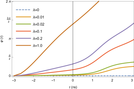
Figure 3: The pulse phase $\varphi(\tau)$ as a function of the local time $\tau$. The dashed line that corresponds to zero environmental influence serves as a reference. 

We observe that the variation of the phase closely reflects the variation of the enveloped area. At one extreme with $\lambda=0$, an SIT solitonic pulse does not experience any phase change throughout the propagation, as the vanishing $\lambda$ results in a zero RHS of Eq. (11), producing a constant $\varphi$. At the other extreme with $\lambda=1$, the phase variation almost follows a diagonal asymptote in the $\varphi$-$\tau$ plane, similar to the area variation in the $\theta$-$\tau$ plane. With a large $\lambda$, the exponential factor in Eq. (13) approaches zero, leading to a constant $\mathcal{E}=\dot{\theta}/\mu=\sqrt{8}M/\lambda\mu$ as well as a constant slope $\dot{\varphi}=M\lambda/\sqrt{8}$ when the propagated area $\theta$ is sufficiently large according to Eq. (11). For other values of $\lambda$, we note two stages of phase variations in general, the separating point of which follows the time point the qubit obtains full inversion as discussed in the last section.

V Conclusions

We have studied the variations of the envelope and the phase of a microwave pulse during its propagation along a waveguide through a qubit on a superconducting circuit. The study is given under the presence of a dissipative environment which we have assumed to have a frictive spectral distribution. Modelling on a coupled Maxwell-master equation, we show that solution is admissible for one-shot pulses, where omission of the environment reduces the solution to a symmetric soliton familiar to classical SIT effects. The dissipative pulses have asymmetric and multi-peak shapes, depending on the scale factor of the frictive environment. We have given detailed analysis on these shapes in both the aspects of envelope and phase. Such detailed knowledge would benefit the design of more sophisticated pulses to control the qubit state for the purpose of storing and processing quantum information.

- (1) J. Clarke and F. K. Wilhelm, Nature 453, 1031 (2008).
- (2) J. Q. You and F. Nori, Nature 474, 589 (2011).
- (3) H. Ian, Y. Liu, and F. Nori, Phys. Rev. A 81, 063823 (2010).
- (4) J. M. Martinis, K. B. Cooper, R. McDermott, M. Steffen, M. Ansmann, K. D. Osborn, K. Cicak, S. Oh, D. P. Pappas, R. W. Simmonds, and C. C. Yu, Phys. Rev. Lett. 95, 210503 (2005).
- (5) J. M. Martinis, S. Nam, J. Aumentado, K. M. Lang, and C. Urbina, Phys. Rev. B 67, 094510 (2003).
- (6) R. C. Bialczak, R. McDermott, M. Ansmann, M. Hofheinz, N. Katz, E. Lucero, M. Neeley, A. D. O’Connell, H. Wang, A. N. Cleland, and J. M. Martinis, Phys. Rev. Lett. 99, 187006 (2007).
- (7) F. Yoshihara, K. Harrabi, A. O. Niskanen, Y. Nakamura, and J. S. Tsai, Phys. Rev. Lett. 97, 167001 (2006).
- (8) G. Ithier, E. Collin, P. Joyez, P. J. Meeson, D. Vion, D. Esteve, F. Chiarello, A. Shnirman, Y. Makhlin, J. Schriefl, and G. Sch n, Phys. Rev. B 72, 134519 (2005).
- (9) F. Mallet, F. R. Ong, A. Palacios-Laloy, F. Nguyen, P. Bertet, D. Vion, and D. Esteve, Nat. Phys. 5, 791 (2009).
- (10) S. Yu, Y. Gao, and H. Ian, Quant. Inf. Process. 16, 283 (2017).
- (11) L. Tian, S. Lloyd, and T. P. Orlando, Phys. Rev. B 65, 144516 (2002).
- (12) J. Q. You, X. Hu, S. Ashhab, and F. Nori, Phys. Rev. B 75, 140515 (2007).
- (13) R. McDermott, IEEE Trans. Appl. Supercond. 19, 2 (2009).
- (14) A. O. Caldeira and A. J. Leggett, Ann. Phys. 149, 374 (1983).
- (15) A. J. Leggett, Phys. Rev. B 30, 1208 (1984).
- (16) L. F. Wei, Y. Liu, and F. Nori, Phys. Rev. Lett. 96, 246803 (2006).
- (17) M. Neeley, R. C. Bialczak, M. Lenander, E. Lucero, M. Mariantoni, A. D. O’Connell, D. Sank, H. Wang, M. Weides, J. Wenner, Y. Yin, T. Yamamoto, A. N. Cleland, and J. M. Martinis, Nature 467, 570 (2010).
- (18) A. O. Caldeira and A. J. Leggett, Phys. Rev. Lett. 46, 211 (1981).
- (19) A. Widom and T. D. Clark, Phys. Rev. Lett. 48, 63 (1982).
- (20) Y. Gao, S. Jin, and H. Ian, arXiv: 1811.05126 (2018).
- (21) N. G. Basov, R. V. Ambartsumyan, V. S. Zuev, P. G. Kryukov, and V. S. Letokhov, Soviet JETP 23, 16 (1966).
- (22) S. L. McCall and E. L. Hahn, Phys. Rev. Lett. 18, 908 (1967).
- (23) C. Eichler, C. Lang, J. M. Fink, J. Govenius, S. Filipp, and A. Wallraff, Phys. Rev. Lett. 109, 240501 (2012).
- (24) P. Y. Wen, A. F. Kockum, H. Ian, J. C. Chen, F. Nori, and I.-C. Hoi, Phys. Rev. Lett. 120, 063603 (2018).
- (25) P. Y. Wen, K.-T. Lin, A. F. Kockum, B. Suri, H. Ian, J. C. Chen, S. Y. Mao, C. C. Chiu, P. Delsing, F. Nori, G.-D. Lin, and I.-C. Hoi, Phys. Rev. Lett. 123, 233602 (2019).