ElasTool: An automated toolkit for elastic constants calculation

Abstract

We here present, the ElasTool package, an automated toolkit for calculating the second-order elastic constants (SOECs) of any two- (2D) and three-dimensional (3D) crystal systems. It can utilize three kinds of strain-matrix sets, the high-efficiency strain-matrix sets (OHESS), the universal linear-independent coupling strains (ULICS) and the all-single-element strain-matrix sets (ASESS) to calculate the SOECs automatically. In an automatic manner, ElasTool can deal with both zero- and high-temperature elastic constants. The theoretical background and computational method of elastic constants, the package structure, the installation and run, the input/output files, the controlling parameters, and two representative examples of ElasTool are described detailedly. ElasTool is useful for either the exploration of materials’ elastic properties or high-throughput new materials design. ElasTool is also available at our website: www.matdesign.cn.

PROGRAM SUMMARY
Program Title: ElasTool
Licensing provisions: GNU General Public License, version 3
Programming language: Python 3
Computer: Any computer that can run Python (versions 3.5 and later).
Operating system: Any operating system that can run Python.
External routines: NumPy [1], Spglib [2], ASE [3], Pandas [4]
Nature of problem: The stress-strain method of elastic constants calculation depends on more accurate stresses calculated by density functional theory (DFT) compared to the strain-energy method. But its advantage is that it needs a smaller number of strain sets to solve the equation sets to deduce elastic constants and more straightforward to implement. While the more accurate stresses take much more time in DFT calculating. Thus, a smaller number of strain sets and more efficient strain sets are urgently needed to improve the computational efficiency of elastic constants. An automated solution coupled with DFT is necessary for the exploration of materials’ elastic properties and high-throughput new materials design.
Solution method: The solution to improving the computational efficiency of the stress-strain method is to decrease the number of strain-matrix sets and optimize the strain-matrix sets. We coupled our previously proposed high-efficiency strain-matrix sets (OHESS) with DFT and automated the processes of the calculation of the elastic constants using the stress-strain method in the ElasTool package. ElasTool can also adopt the all-single-element strain-matrix sets (ASESS) and the universal linear-independent coupling strains (ULICS). It can deal with both zero- and high-temperature elastic constants of any crystal systems belonging to 2D or 3D. It can also output other elastic moduli, the elastic anisotropy, Debye temperature, the sound velocities, and elastic stability based on the calculated elastic constants.
Additional comments: This package can use the stress tensors calculated by other DFT codes, such as the Vienna Ab initio Simulation Package (VASP) [5, 6, 7].
Running time: The time used by the examples provided in the distribution mainly spends on the DFT parallel running.  

1 Introduction

Elastic constants are fundamental parameters of materials, which are crucial to many disciplines, including physics [1], condensed matter, materials science (Ref. [2]), geophysics [3], and chemical [4]. In new materials’ theoretical design aided by crystal structure prediction [5, 6, 7, 8, 9, 10], elastic constants are frequently used to check the stability of the predicted structures, according to Born elastic stability criteria [11, 12, 13, 14, 15, 16]. More interestingly, for the informatics-based new materials screening and design, elastic constants are important properties and have been extensively calculated and collected in some materials database, such as the Materials Project (MP) [17] and JARVIS-DFT [18] databases.

The high-accuracy state of the art density functional theory (DFT) [19, 20] is capable of calculating elastic constants accurately. For the calculation method, generally, there are two ways to calculate elastic constants, the energy-strain method and the stress-strain method (Refs. [21, 22, 23] and references therein). Compared to the former, the latter depends on highly accurate stress tensors but a smaller number of strain sets [22, 21]. The high-accuracy stress tensors calculation always needs higher energy cutoff and denser K-point meshes. Although it is much more computationally expensive and time-consuming, it is simple to implement and straightforward to calculate the high-pressure elastic constants of materials without pressure corrections, unlike the the strain-energy method which needs complex pressure corrections [24].

Our previously proposed OHESS can keep the symmetry of strained crystal to the most extent and largely lower computation time at the same level of accuracy [25]. This method is integrated into the ElasTool package, which can calculate the SOECs of any crystal systems belonging to 2D and 3D. ElasTool can also uses the ULICS [16] to calculate elastic constants. However, in the ULICS, the coupling of stress components by including several strain components at the same time will largely reduce the symmetry of the strained crystal. This will greatly lengthen the computation time [25]. ElasTool has also integrated the ASESS, in which only one strain component is applied on crystal lattice in a certain strain-matrix set.

The rest of this paper is arranged as follows. The theoretical background of elasticity is presented in the next section. The descriptions of the package are detailed in Sec. 3. The input and output files are described in Sec. 4. Input parameters are explained in Sec. 5. The calculation examples are shown in Sec. 6. Section 7 is a summary of this paper.

2 Theoretical background of elasticity

2.1 Elastic constants computation method

Within the linear elastic regime of a crystal, the relation between the stresses $\sigma_{i}$ and corresponding strains $\varepsilon_{j}$ conforms to Hooke’s law,

$$\sigma_{i}=\sum_{j=1}^{6}C_{ij}\varepsilon_{j}$$ (1)

where the coefficient $C_{ij}$ are the elastic stiffness constants of the crystal.

If we deform a crystal by applying the strain $\varepsilon_{j}$ and calculate the corresponding stresses, we can obtain its elastic constants from Eq.1. The deformation matrix applied to the crystal unit cell is

$$\boldsymbol{D}=\boldsymbol{I}+\boldsymbol{\varepsilon},$$ (2)

where $\boldsymbol{I}$ is the $3\times 3$ unit matrix, and $\boldsymbol{\varepsilon}$ is the strain-matrix notated by Voigt method. In the 3D case, the strain matrix is

$$\boldsymbol{\varepsilon}=\left[\begin{array}[]{l}\varepsilon_{1}\quad{\varepsilon_{6}}/{2}\quad{\varepsilon_{5}}/{2}\\ {\varepsilon_{6}}/{2}\quad\varepsilon_{2}\quad{\varepsilon_{4}}/{2}\\ {\varepsilon_{5}}/{2}\quad{\varepsilon_{4}}/{2}\quad\varepsilon_{3}\end{array}\right].$$ (3)

For the 2D layered crystal, ElasTool assumes the crystal plane in the $xy$ plane and the strain matrix is

$$\boldsymbol{\varepsilon}=\left[\begin{array}[]{l}\varepsilon_{1}\quad{\varepsilon_{6}}/{2}\quad 0\\ {\varepsilon_{6}}/{2}\quad\varepsilon_{2}\quad 0\\ 0\qquad 0\quad 0\end{array}\right].$$ (4)

After deformation, the crystal lattice vector is

$$\boldsymbol{A}^{\prime}=\boldsymbol{A}\cdot\boldsymbol{D}$$ (5)

where $\boldsymbol{A}$ is the original crystal lattice vector.

The SOECs can be readily derived by fitting the first-order function to the stress-strain data according to Eq.1.

2.2 Strain matrix sets

In order to extract all SOECs of a crystal belonging to a specific crystal system, we need deformation matrices defined by a set of strain matrices to apply on the crystal lattice. We previously proposed the OHESS and finally improved the computational efficiency of elastic constants considerably, as reported in Ref. [25]. ElasTool uses three kinds of strain-matrix sets, the OHESS, the ASESS, and the ULICS to solve the stress-strain equation sets to find the corresponding elastic constants numerically. The ASESS is defined in Ref. [25]. As for the details of the ULICS, the readers are referred to as Ref. [16]. Overall, the OHESS has the highest efficiency among the three kinds of strain-matrix sets, as has been tested in Ref. [25].

2.3 Elastic moduli

From the calculated elastic constants, we can derive other elastic moduli easily. The Voigt and Reuss bulk and shear moduli for different crystal systems are calculated according to Ref. [11]. From the Voigt–Reuss–Hill approximations [26], the arithmetic average of Voigt and Reuss bounds is written as

$$B_{\operatorname{VRH}}=\frac{B_{V}+B_{R}}{2},$$ (6)

and

$$G_{\operatorname{VRH}}=\frac{G_{V}+G_{R}}{2},$$ (7)

respectively.

Young’s modulus $E$ is obtained by

$$E=\frac{9BG}{3B+G},$$ (8)

and Poisson’s ratio is

$$\nu=\frac{3B-2G}{2(3B+G)}.$$ (9)

The elastic anisotropy is a crucial measurement of anisotropy of chemical bonding. The Chung-Buessem anisotropy index [27] is defined as

$$A^{C}=\frac{G_{V}-G_{R}}{G_{V}+G_{R}}$$ (10)

The universal elastic anisotropy index proposed by Ranganathan and Ostoja-Starzewski [28] is

$$A^{U}=5\frac{G_{V}}{G_{R}}-\frac{B_{V}}{C_{R}}-6\geqslant 0$$ (11)

2.4 Sound velocity

The phase velocity $v$ and polarization of the three waves along a fixed propagation direction defined by the unit vector $n_{i}$ are given by Cristoffel equation

$$(C_{ijkl}n_{j}n_{k}-\rho v^{2}\delta_{ij})u_{i}=0$$ (12)

where $C_{ijkl}$ is the fourth-rank tensor description of the elastic constants, $n$ is the propagation direction, and $u$ the polarization vector.

The longitudinal wave velocity is defined by

$$v_{P}=\sqrt{\frac{B+4G/3}{\rho}},$$ (13)

and the body wave velocity is

$$v_{B}=\sqrt{\frac{B}{\rho}}.$$ (14)

The shear wave velocity is written as

$$v_{S}=\sqrt{\frac{G}{\rho}}.$$ (15)

From $v_{S}$ and $v_{P}$, we can average wave velocity via

$$v_{m}=\left[\frac{1}{3}\left(\frac{2}{v_{S}^{3}}+\frac{1}{v_{P}^{3}}\right)\right]^{-1/3}.$$ (16)

From elastic constant data we can calculate the Debye temperature from the average sound velocity $v_{m}$ via

$$\Theta_{D}=\frac{h}{k}\left[\frac{3n}{4\pi}\left(\frac{N_{A}\rho}{M}\right)\right]^{1/3}v_{m}$$ (17)

where $h$ is Planck’s constant, $k$ the Boltzmann’s constant, $N_{A}$ the Avogadro’s number, $n$ the number of atoms in the unit cell, $M$ the weight of the unit cell, and $\rho$ the density.

3 Description of the package

3.1 The flowchart of ElasTool

The flowchart of ElasTool package is illustrated in Fig.1. First, ElasTool reads the crystal structure file in either POSCAR or cif format, and calls VASP [29, 30] to optimize the initial structure at fixed pressure or volume specified in the INCARs file. For the optimized crystal lattice, ElasTool then applies different types of deformation matrices according to its symmetry and optimizes all atoms’ positions. Then, all the stress tensors corresponding to each deformation matrix are calculated and collected. Subsequently, ElasTool fits the first-order function to the collected stress-strain data to deduce the full elastic constants. The elastic moduli are calculated according to Eqs. 6-9. The Debye temperature is calculated from Eq. 17. The sound velocity is calculated from Eq. 13-16. The elastic anisotropy is analyzed by Eqs. 10 and 11. The mechanical stability of this crystal structure is analyzed according to Born stability criteria proposed in Refs. [11, 12]. Finally, ElasTool stores all the data calculated to the elastool.out file and exits.

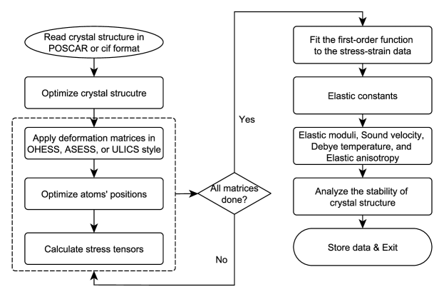
Figure 1: The flowchart of ElasTool

3.2 Installation requirements

ElasTool is based on Python and its installation is very easy. But before the installation of ElasTool, the necessary libraries should be installed first. The following packages are required:

$\bullet$ Python3.5 or later.

$\bullet$ NumPy.

$\bullet$ Spglib.

$\bullet$ ASE.

$\bullet$ Pandas.

$\bullet$ VASP.

Python 3 is the basic language environment for ElasTool running. Numpy is for numerical calculations. Spglib is for the automatic determination of symmetry of crystal structure. ASE is used to manipulate the crystal structures. Pandas is for the statistics of stress tensors calculated. At present, ElasTool interfaces to VASP package for calculating the accurate stresses of strained crystal. But the interfaces to other DFT packages can also be easily implemented.

3.3 Installation

In the Python 3 environment, the necessary libraries can be installed via pip command, e.g., pip install numpy. For the construction of the environment and libraries, the miniconda3 management platform of Python packages is highly recommended. After installing miniconda3, the basic Python 3 language environment is constructed and the other libraries can be installed via either conda or pip commands. For example, one can install numpy via conda install -c conda-forge numpy.

3.4 Run

To run ElasTool, one only needs to execute elastool in the working directory. ElasTool will automatically prepare necessary files for calculating the stresses of crystal under deformation, and then call VASP to optimize initial crystal structure and calculate the stresses for each deformation defined by OHESS, ASESS, or ULICS. Finally, ElasTool analyzes the stress-strain relationship according to Hooke’s law and calculates all the elastic constants.

4 Input/output files

4.1 Input files

ElasTool needs one main input file for setting the calculation details of elastic constants. The main input file is named elatool.in. The crystal structure file is provided either in POSCAR or cif format for reading in the structure information of the crystal. For VASP stress tensor calculations, INCARs, KPOINTS-static, KPOINTS-dynamic, and POTCAR-XX files are also necessary. In the INCARs file, several INCAR files of VASP are collected for optimization, the static calculation, and the molecular dynamics simulations of high-temperature elastic constants. The KPOINTS-static file is for the structure optimization and the static calculation of stress tensors. The KPOINTS-dynamic file is for the calculation of high-temperature elastic constants using molecular dynamics. XX in the POTCAR file name is the abbreviated name for an element of the crystal.

5 Input parameters

There are totally 10 controlling parameters of ElasTool, as listed in Table.1. The run_mode sets the running mode for ElasTool, 1 for automatic run, 2 for pre-processing, and 3 for post-processing. If run_mode = 2 or 3, one should ensure the structure has already been optimized at fixed pressure or volume, i.e. both the CONTCAR and OUTCAR files are in ./OPT directory. In running mode 2, ElasTool will directly prepare all the necessary files for calculating stress tensors. After all the stress tensors calculations are finished, run mode 3 can analyze the output files and extract stress tensors, and then fit the first-order function to the stress-tensor data to obtain elastic constants. The dimensional defines the dimensional of the system, 2D or 3D. If the system is 2D, ElasTool supposes the layered sheet in the xy-plane. The structure_file specifies the original crystal structure file in POSCAR (.vasp) or cif (.cif) format. The if_conventional_cell determines the usage of primitive cell (no) or conventional cell (yes). The method_stress_statistics chooses the elastic constants calculation method, static or dynamic, static for 0 K elastic constants, dynamic for high-temperature. The static method uses the static stress to compute elastic constants, while the dynamic method deduces elastic constants from the thermal stresses obtained by molecular dynamics simulations. The strains_matrix defines the type of strain-matrix set, OHESS, ASESS, or ULICS. The strains_list gives one or more strains for calculating stresses via the strain-matrix set of OHESS, ASESS, or ULICS. The repeat_num controls how to build a supercell from the primitive or conventional cell defined by if_conventional_cell for the dynamic method. The num_last_samples is the number of last MD steps to average thermal stresses. The parallel_submit_command is the parallel submitting command of ab initio code, e.g. VASP.

Table 1: The controlling parameters and possible values of ElasTool

Parameters	Values
run_mode	1/2/3
dimensional	2D/3D
structure_file	file name ended with .vasp or .cif
if_conventional_cell	yes/no
method_stress_statistics	static/dynamic
strains_matrix	ohess/asess/ulics
strains_list	one or more numbers
repeat_num	3 integers
num_last_samples	1 integer
parallel_submit_command	DFT parallel run command

6 Example of run

The best way to learn ElasTool is to start from the examples. ElasTool can calculate zero-temperature and high-temperature elastic constants. The zero-temperature calculations can be conducted by static stress computation. The high-temperature elastic constants can be derived by molecular dynamics simulations.

6.1 Zero-temperature elastic constants

We take the 0 K elastic constants calculation of diamond as the static example. The content of the input file elastool.in is as follows.

run_mode = 1

dimensional = 3D

structure_file = diamond.cif

if_conventional_cell = no

method_stress_statistics = static

strains_matrix = ohess

strains_list = -0.06 -0.03 0.03 0.06

#repeat_num = 1 1 1

#num_last_samples = 1

parallel_submit_command = mpirun -np 28 vasp544

6.2 High-temperature elastic constants

The high-temperature elastic constants calculation of metal copper is the high-temperature example. We build a $3\times 3\times 3$ supercell from the conventional cell of face-centered-cubic of Cu and then perform long-time MD simulations defined in the INCAR-dynamic file. Because MD is very time consuming, there is only one strain of -0.06 is used. The last 500 MD steps are used to average thermal stresses.

run_mode = 1

dimensional = 3D

structure_file = CONTCAR.vasp

if_conventional_cell = yes

method_stress_statistics = dynamic

strains_matrix = ohess

strains_list = -0.06

repeat_num = 3 3 3

num_last_samples = 500

parallel_submit_command = mpirun -np 28 vasp544

6.3 Output files

The elastool.out file is the unique output file of ElasTool. It includes the calculated elastic constants data, the elastic moduli, the sound velocity, the Debye temperature, the elastic anisotropy, and the stability analysis results of the crystal structure based on Born elastic criteria. The printed information on the screen of the diamond example is as follows.

Reading controlling parameters from elastool.in...

Calculating stresses using the OHESS strain matrices...

strain = -0.060

strain = -0.030

strain = 0.030

strain = 0.060

Fitting the first-order function to the collected

stress-strain data according to Hooke’s law...

The finnal results are as follows:

+==========================================+

|This is a 3D Cubic lattice.               |

|-------------------------------------------|

|Mean Pressure = -0.08 GPa                  |

|-------------------------------------------|

|Elastic constants:                        |

|C11 = 1055.04 GPa                          |

|C12 = 136.56 GPa                           |

|C44 = 567.76 GPa                           |

|-------------------------------------------|

|Elastic moduli:                           |

|B_V = 442.72 GPa                           |

|B_R = 442.72 GPa                           |

|G_V = 524.36 GPa                           |

|G_R = 518.73 GPa                           |

|B_VRH = 442.72 GPa                         |

|G_VRH = 521.54 GPa                         |

|Young’s modulus (E) = 1123.47 GPa          |

|Possion’s ratio (V) = 0.0771               |

|-------------------------------------------|

|Sound velocity:                            |

|V_S = 12.20 Km/s                           |

|V_B = 11.24 Km/s                           |

|V_P = 18.03 Km/s                           |

|V_M = 13.31 Km/s                           |

|-------------------------------------------|

|Debye temperature:                        |

|T_D = 1761.03 K                            |

|-------------------------------------------|

|Elastic anisotropy:                       |

|A_U = 0.0542                               |

|A_C = 0.0054                               |

|-------------------------------------------|

|Structure stability analysis...           |

|This structure is mechanically STABLE.      |

+==========================================+

Results are also saved in the elastool.out file.

Well done! GOOD LUCK!

7 Conclusions

In summary, we here introduced the automatic calculation toolkit of second-order elastic constants, ElasTool. First, we recalled the theoretical background and computation method of elastic constants, elastic moduli, sound velocity, elastic anisotropy, and Debye temperature. Then, we described the structure of ElasTool package and its installation. Subsequently, we detailed the necessary input files and the controlling parameters of ElasTool. Finally, the calculation examples of 0 K and high-temperature elastic constants are illustrated in detail. The running output of ElasTool is also presented. Overall, we developed a useful toolkit for calculating elastic constants, as is of great significance for either the exploration of materials’ elasticity or high-throughput new materials design.

8 Acknowledgments

We acknowledge the support from the National Natural Science Foundation of China (41574076), the Key Research Scheme of Henan Universities (18A140024), and the Research Scheme of LYNU Innovative Team under Grant No. B20141679.

References

- [1] https://numpy.org/
- [2] https://atztogo.github.io/spglib/
- [3] https://wiki.fysik.dtu.dk/ase/
- [4] https://pandas.pydata.org/
- [5] https://www.vasp.at/
- [6] G. Kresse, J. Furthmüller, Efficient iterative schemes for ab initio total-energy calculations using a plane-wave basis set, Phys. Rev. B 54 (1996) 11169.
- [7] G. Kresse, D. Joubert, From ultrasoft pseudopotentials to the projector augmented-wave method, Phys. Rev. B 59 (1999) 1758.

References

- [1] N. W. Ashcroft, N. D. Mermin, Solid State Physics, Harcourt College Publishers, New York, 1976.
- [2] A. M. Tehrani, J. Brgoch, Hard and superhard materials: A computational perspective, J. Solid State Chem. 271 (2019) 47. doi:10.1016/j.jssc.2018.10.048.
- [3] T. Lay, T. C. Wallace, Modern Global Seismology, Elsevier Inc., Amsterdam, 1995.
- [4] K. Tatsumi, I. Tanaka, K. Tanaka, H. Inui, M. Yamaguchi, H. Adachi, M. Mizuno, Elastic constants and chemical bonding of LaNi5 and LaNi5h7 by first principles calculations, J. Phys.: Condens. Matt. 15 (2003) 6549. doi:10.1088/0953-8984/15/38/021.
- [5] Z. L. Liu, Muse: Multi-algorithm collaborative crystal structure prediction, Comput. Phys. Commun. 185 (2014) 1893. doi:10.1016/j.cpc.2014.03.017.
- [6] Y. Wang, J. Lv, L. Zhu, Y. Ma, Crystal structure prediction via particle-swarm optimization, Phys. Rev. B 82 (2010) 094116. doi:10.1103/PhysRevB.82.094116.
- [7] Y. Wang, J. Lv, L. Zhu, Y. Ma, Calypso: A method for crystal structure prediction, Comput. Phys. Commun. 183 (2012) 2063. doi:10.1016/j.cpc.2012.05.008.
- [8] C. W. Glass, A. R.Oganov, N. Hansen, Uspex—evolutionary crystal structure prediction, Comput. Phys. Commun. 175.
- [9] D. C. Lonie, E. Zurek, Xtalopt: An open-source evolutionary algorithm for crystal structure prediction, Comput. Phys. Commun. 182.
- [10] C. J. Pickard, R. J. Needs, Ab initio random structure searching, J. Phys.: Condens. Matt. 23.
- [11] Z. J. Wu, E. J. Zhao, H. P. Xiang, X. F. Hao, X. J. Liu, J. Meng, Crystal structures and elastic properties of superhard and from first principles, Phys. Rev. B 76 (2007) 054115. doi:10.1103/PhysRevB.76.054115.
- [12] F. Mouhat, F. X. Coudert, Necessary and sufficient elastic stability conditions in various crystal systems, Phys. Rev. B 90 (2014) 224104. doi:10.1103/PhysRevB.90.224104.
- [13] J. F. Nye, Physical Properties of Crystals, Oxford University Press, Oxford, 1985.
- [14] M. Born, K. Huang, Dynamical Theory of Crystal Lattices, Oxford University Press, Oxford, 1954.
- [15] Z. L. Liu, H. Jia, R. Li, X. L. Zhang, L. C. Cai, Unexpected coordination number and phase diagram of niobium diselenide under compression, Phys. Chem. Chem. Phys. 19 (2017) 13219. doi:10.1039/c7cp00805h.
- [16] R. Yu, J. Zhu, H. Q. Ye, Calculations of single-crystal elastic constants made simple, Comput. Phys. Commun. 181 (2010) 671. doi:10.1016/j.cpc.2009.11.017.
- [17] M. D. Jong, W. Chen, T. Angsten, A. Jain, R. Notestine, A. Gamst, M. Sluiter, C. K. Ande, S. van der Zwaag, J. J. Plata, C. Toher, S. Curtarolo, G. Ceder, K. A. Persson, M. Asta, Charting the complete elastic properties of inorganic crystalline compounds, Scientific Data 2 (2015) 150009. doi:10.1038/sdata.2015.9.
- [18] K. Choudhary, G. Cheon, E. Reed, F. Tavazza, Elastic properties of bulk and low-dimensional materials using van der waals density functional, Phys. Rev. B 98.
- [19] P. Hohenberg, W. Kohn, Inhomogeneous electron gas, Phys. Rev. 136 (1964) B864. doi:10.1103/PhysRev.136.B864.
- [20] W. Kohn, L. J. Sham, Self-consistent equations including exchange and correlation effects, Phys. Rev. 140 (1965) A1133. doi:10.1103/PhysRev.140.A1133.
- [21] V. Wang, N. Xu, J. C. Liu, G. Tang, W. T. Geng, Vaspkit: A pre- and post-processing program for vasp code (arxiv:1908.08269v2) (2019). arXiv:arXiv:1908.08269.
- [22] R. Golesorkhtabar, P. Pavone, J. Spitaler, P. Puschnig, C. Draxl, Elastic: A tool for calculating second-order elastic constants from first principles, Comput. Phys. Commun. 184 (2013) 1861. doi:10.1016/j.cpc.2013.03.010.
- [23] W. F. Perger, J. Criswell, B. Civalleri, R. Dovesi, Ab-initio calculation of elastic constants of crystalline systems with the crystal code, Comput. Phys. Commun. 180 (2009) 1753. doi:10.1016/j.cpc.2009.04.022.
- [24] G. V. Sin’ko, N. A. Smirnov, Ab initio calculations of elastic constants and thermodynamic properties of bcc, fcc, and hcp al crystals under pressure, J. Phys.: Condens. Matter 14 (2002) 6989. doi:10.1088/0953-8984/14/29/301.
- [25] Z. L. Liu, High-efficiency calculation of elastic constants enhanced by the optimized strain-matrix sets(arxiv:2002.00005) (2020). arXiv:arXiv:2002.00005.
- [26] R. Hill, The elastic behaviour of a crystalline aggregate, Proc. Phys. Soc. London , 350 65.
- [27] D. H. Chung, W. R. Buessem, The elastic anisotropy of crystals, J. of Appl. Phys. 38.
- [28] S. I. Ranganathan, M. Ostoja-Starzewski, Universal elastic anisotropy index, Phys. Rev. Lett. 101.
- [29] G. Kresse, J. Furthmüller, Efficient iterative schemes for ab initio total-energy calculations using a plane-wave basis set, Phys. Rev. B 54 (1996) 11169. doi:10.1103/PhysRevB.54.11169.
- [30] G. Kresse, D. Joubert, From ultrasoft pseudopotentials to the projector augmented-wave method, Phys. Rev. B 59 (1999) 1758. doi:10.1103/PhysRevB.59.1758.