Avoiding the sign-problem in lattice field theory

Abstract

In lattice field theory, the interactions of elementary particles can be computed via high-dimensional integrals. Markov-chain Monte Carlo (MCMC) methods based on importance sampling are normally efficient to solve most of these integrals. But these methods give large errors for oscillatory integrands, exhibiting the so-called sign-problem. We developed new quadrature rules using the symmetry of the considered systems to avoid the sign-problem in physical one-dimensional models for the resulting high-dimensional integrals. This article gives a short introduction to integrals used in lattice QCD where the interactions of gluon and quark elementary particles are investigated, explains the alternative integration methods we developed and shows results of applying them to models with one physical dimension. The new quadrature rules avoid the sign-problem and can therefore be used to perform simulations at until now not reachable regions in parameter space, where the MCMC errors are too big for affordable sample sizes. However, it is still a challenge to develop these techniques further for applications with physical higher-dimensional systems.

1 Introduction

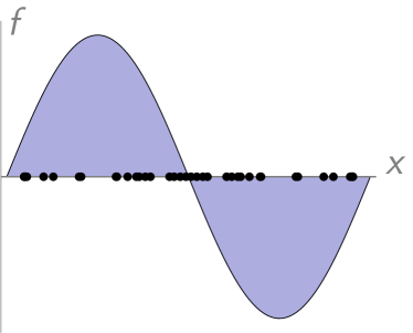
Monte Carlo (MC) methods are in general very efficient to solve high-dimensional integrals. They use the law of large numbers to approximate an integral with quadrature rules that use random sampling points. But MC methods are highly inefficient for oscillatory integrand functions, e.g. the function shown in Figure 1a. An exact integration of oscillatory functions would, of course, result in the cancellation of large negative and positive contributions to the integral - in the example in Figure 1a this would give an integral of zero. However, the random choice of sampling points in MC methods, shown as black points in Figure 1a, does lead only to approximate cancellation when the number of points is relatively big and hence, it is very difficult to obtain accurate results with affordable sample sizes. This non-perfect cancellation of negative and positive parts in the integration method, usually resulting in large quadrature rule errors, is called the sign-problem. The sign-problem is for example the reason why important physical interactions in the early universe cannot be simulated which could explain why there is more matter than anti-matter in our universe today. To acquaint better knowledge of these fundamental phenomena, it is essential to develop alternative quadrature rules to MC that avoid the sign-problem.

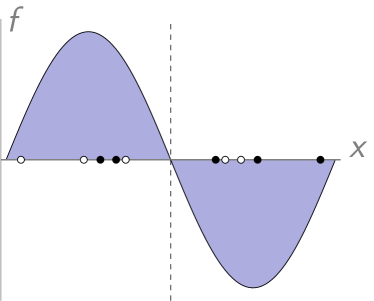
In physical applications, the function to-be-integrated describes some characteristic in a given physical model. We investigated methods that use some symmetry of the physical model to result in the exact cancellation of positive and negative parts in the quadrature rule. If the model behind the function in Figure 1b has a reflection symmetry, few MC sampling points - in black - can be chosen and together with their reflected - white - points they form a set of sampling points that results in an exact quadrature rule. In this specific example even one MC point with its reflection point would give an exact result, for more complicated functions more sampling points are needed.

(a) MC sampling points

(b) Symmetric sampling points

Figure 1: MC integration of an oscillatory function results in large errors, known as the sign-problem. This problem is due to the non-cancellation of positive and negative contributions to the quadrature rule (a). Choosing sampling points by using the symmetry of the underlying model results in an exact quadrature rule (b).

This article first gives a short introduction to the high-dimensional integrals that have to be solved in particle physics, more precisely in lattice QCD. Readers that are mostly interested in the integration methods can easily skip this part. The main part of this article presents the methods we developed and tested to avoid the sign-problem for high-dimensional integration in physical one-dimensional systems.

We found that symmetrically chosen quadrature rules can avoid the sign-problem and can efficiently be applied also to high-dimensional integrals. These rules can help to perform simulations in important, not-yet reachable regions in parameter space, at least in physical one-dimensional systems so far. To apply them to higher physical dimensions, in particular to physical four-dimensional systems in high energy physics as lattice QCD, they clearly need to be developed further.

2 Integration in lattice QCD

In theoretical physics the interaction between elemetary particles such as the electron, is described by quantum field theories (QFT), see e.g. Peskin:1995ev . The mathematical formalism in QFT defines particles as classical fields that are functions in three space dimensions and one time dimension, $P(x,y,z,t)$. Operators, $O[P]$, are functionals of these fields and describe the interactions between them. An expectation value $A$ of this interaction or operator $O[P]$, also called amplitude, is computed via the path integral,

$$A=\frac{\int O[P]B[P]\,\text{d}P}{\int B[P]\,\text{d}P}.$$ (1)

$\int\!\text{d}P\,$ is the infinite-dimensional integration over all possible states of the field $P$ in time and space. The path integral becomes a well defined expression, if a Euclidean metric is used and the fields are defined on a finite dimensional, discrete lattice. In (1), $B[P]$ is called the Boltzmann-weight and provides a probability which weights the particle (field) interactions. The denominator in (1) insures the proper normalization of $A$. The expectation value $A$ is interesting because physical observables can be derived from it and their numerical values can be compared with experimental results or can give new results that are not yet possible to reach with experiments.

In lattice field theory, space-time and the involved functionals $O[P]$ and $B[P]$ are discretized in Euclidean space, such that (1) can be computed numerically. Often, the Boltzmann-weight is a highly peaked function suggesting that this computation can be done using importance sampling techniques. In most computations, this importance sampling is done by a Markov chain MC (MCMC) algorithm using a Markov chain that leaves the distribution density $\frac{B[P]}{\int B[P]\text{d}P}$ invariant. To compute $A$ numerically, four-dimensional space-time is discretized on a four-dimensional lattice with four directions $\mu\in\{1,2,3,4\}$ , lattice sites $\bm{n}\in\Lambda=\{(n_{1},n_{2},n_{3},n_{4})|n_{1},n_{2},n_{3},n_{4}\in\{1,...,d\}\}$ and discretized fields $P$. This results in an $4d$-dimensional integration over the Haar measure of the compact group $\mathcal{SU}(3)$. For real applications, $d$ can be very large, reaching orders of magnitude of several thousands nowadays. Thus, we are left with an extremely high dimensional integration problem. Moreover, for some physically very important questions MCMC methods cannot be applied succesfully. This concerns, for example, the very early universe or the matter anti-matter asymmetry which leads to our sheer existence. Thus, a number of interesting questions remain completely unanswered and it is exactly here where new high dimensional integration methods could be extremely helpful

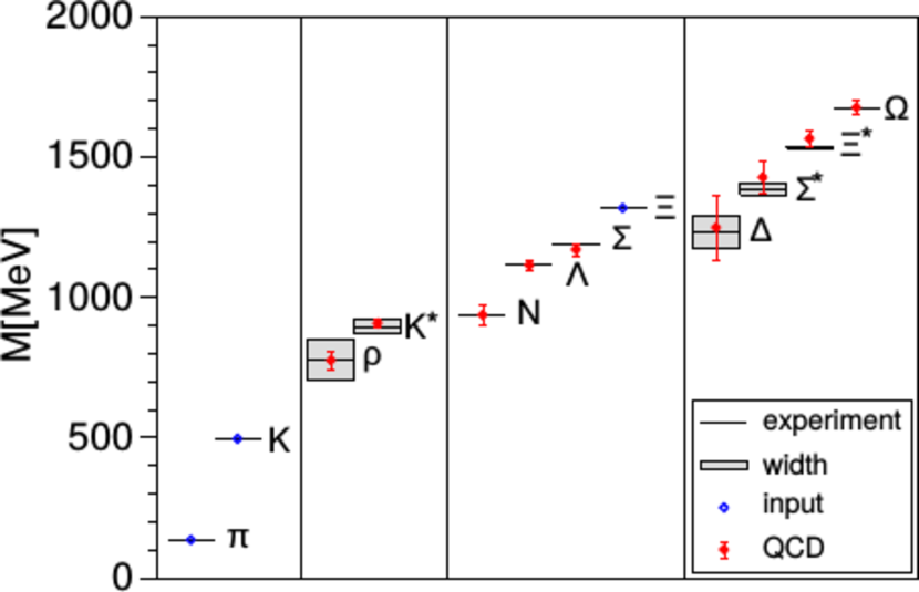
Still, the MCM methods have led to very successful computations already. By performing numerical computations on massively parallel super computers a very impressive result of such a lattice MCMC can be obtained: namely, the mass spectrum of the lightest composite particles made out of quarks and gluons that agrees completely with the experimental values, see Figure 2. To get similar precise results for other, more error-prone observables, research is going on to develop new methods to make this high-dimensional integration faster and the results more precise.

Figure 2: The via lattice QCD computed masses of different composite particles (dots with vertical error bars) agree with the experimentally measured values (horizontal lines with error boxes) Durr:2008zz . The masses of $\pi$, $K$ and $\sum$ (dots without error bars) were input values to the computation.

A more detailed introduction to lattice QCD is for example given in the textbooks Gattringer:2010zz ; DeGrand:2006zz ; Rothe:1992nt .

3 Quadrature rules for one-dimensional lattices

In lattice QCD, the amplitude of interactions between quarks and gluons in physical four-dimensional space-time can be computed via a high-dimensional integral using the Haar-measure over the compact group $\mathcal{SU}(3)$, see section 2. This integral is typically solved numerically using MCMC methods. If the integrand is an oscillatory function, this method results in the sign-problem that gives large errors and avoids physical insights in important processes. We developed alternative methods that avoid the sign-problem and at the same time are efficient for high-dimensional integration over compact groups. Due to various complications with physical four-dimensional lattice QCD, we developed and tested the methods for physical one-dimensional models that involve low-dimensional and high-dimensional integration over compact groups. As suggested in section 1, we developed quadrature rules using the symmetry of the models.

This section is structured from low-dimensional to high-dimensional integration: First, it introduces symmetric quadrature rules for one-dimensional integration over compact groups to avoid the sign-problem here. Then, it presents the recursive numerical integration (RNI), a method to reduce high-dimensional integrals to nested one-dimensional integrals. Finally, it shows how to combine both methods to avoid the sign-problem for high-dimensional integration over compact groups. For all three presented methods, the section shows results of applying them to simple physical, one-dimensional models. More detailed explanations of the methods and applications can be found in Volmer2018New .

3.1 Avoiding the sign-problem in physical one-dimensional systems

The sign-problem can already arise in a one-dimensional integration, solving

$$I(f)=\int_{G}f(U)\,\text{d}U$$ (2)

with MC methods over the Haar-measure of $G\in\{\mathcal{U}(N),\mathcal{SU}(N)\}$. Finding an alternative suitable quadrature rule $Q(f)$ ad-hoc to approximate this integral is not straightforward. The articles Bloch:2013ara ; Bloch:2013qva suggest that using symmetrically distributed sampling points can be beneficial for avoiding the sign-problem, possibly resulting in an exact cancellation of positive and negative contributions to the integral, as stated in section 1. The article of Genz genz gives efficient quadrature rules for integrations over spheres, choosing the sampling points symmetrically on the spheres. We searched for measure preserving homeomorphisms to apply the symmetric quadrature rules on spheres to the integration over compact groups. This section describes the two steps to create the symmetric quadrature rules $Q(f)$ for (2):

1. Rewrite the integral $I(f)$ over the compact group $G$ into an integral over spheres. We restricted ourselves to $G\in\{\mathcal{U}(1),\mathcal{U}(2),\mathcal{U}(3),\mathcal{SU}(2),\mathcal{SU}(3)\}$.

2. Approximate each integral over one spheres by a symmetric quadrature rule as proposed in Genz genz , and combine them to a product rule $Q(f)$.

Finally, this section shows results of applying $Q(f)$ to the one-dimensional QCD model with a sign-problem. A more detailed explanation of the method can be found in Ammon:2016jap ; Ammon:2016ztz .

By finding measure preserving homeomorphisms between the compact groups and products of spheres we created polynomially exact quadrature rules for compact groups. The application of these rules to the one-dimensional QCD model gave results on machine precision where the standard MC method shows a sign-problem. Therefore the symmetric quadrature rules avoid the sign-problem and give rise to solve integrals in beforehand non-reachable parameter regions.

Sym 1. Rewriting the integral

The symmetric quadrature rules of Genz genz are designed for the integration over $k$-dimensional spheres $S^{k}$. To use them for the integration over the compact groups $\mathcal{U}(N)$ and $\mathcal{SU}(N)$ with $N\in\{2,3\}$ in (2), the compact groups have to be associated with spheres. The facts that $\mathcal{U}(N)$ is isomorphic to the semidirect product of $\mathcal{SU}(N)$ acting on $\mathcal{U}(1)$ $\big{(}U(N)\cong SU(N)\rtimes U(1)\big{)}$, that $\mathcal{U}(1)$ is isomorphic to $S^{1}$ $\big{(}\mathcal{U}(1)\cong S^{1}\big{)}$ and that $\mathcal{SU}(N)$ is a principal $\mathcal{SU}(N-1)$ bundle over $S^{2N-1}$ result in

$$\mathcal{SU}(N) \simeq S^{3}\times S^{5}\times...\times S^{2N-1},$$ (3)

$$\mathcal{U}(N) \simeq S^{1}\times S^{3}\times...\times S^{2N-1}.$$ (4)

Then, the integral over the Haar-measure of $G$ in (2) can be rewritten as the integral over products of spheres,

$$\int_{G}\!\text{d}U\,f(U)= \int_{S^{2N-1}}\Bigg{(}\int_{S^{2N-3}}\bigg{(}\cdots\int_{S^{n+2}}\Big{(}\int_{S^{n}}$$

$$\qquad\qquad f\big{(}\Phi(\bm{x}_{S^{2N-1}},\bm{x}_{S^{2N-3}},\ldots,\bm{x}_{S^{n+2}},\bm{x}_{S^{n}})\big{)}$$ (5)

$$\qquad\qquad\qquad\qquad\qquad\qquad\text{d}\bm{x}_{S^{n}}\Big{)}\text{d}\bm{x}_{S^{n+2}}\cdots\Big{)}\text{d}\bm{x}_{S^{2N-3}}\Big{)}\text{d}\bm{x}_{S^{2N-1}},$$

with $n=1$ for $\mathcal{U}(N)$ and $n=3$ for $\mathcal{SU}(N)$ Ammon:2016zur . Here, $\bm{x}_{S^{k}}$ is an element on the $k$-sphere and $\Phi:\ \bigtimes_{j}S^{2j-1}\rightarrow G$ with $G\in\{\mathcal{U}(N),\mathcal{SU}(N)\}$ is a measure preserving homeomorphism. We found the homeomorphisms $\Phi_{G}\equiv\Phi$ for the compact groups $G\in\{\mathcal{U}(1),\mathcal{U}(2),\mathcal{U}(3),\mathcal{SU}(2),\mathcal{SU}(3)\}$:

• For $\mathcal{SU}(2)$, $\Phi$ is an isomorphism, given by

  $$\Phi_{\mathcal{SU}(2)}:S^{3} \rightarrow\mathcal{SU}(2),$$

  $$\bm{x} \mapsto\begin{pmatrix}x_{1}+ix_{2}&-(x_{3}+ix_{4})^{*}\\ x_{3}+ix_{4}&\phantom{-}(x_{1}+ix_{2})^{*}\end{pmatrix}.$$ (6)

• For $\mathcal{SU}(3)$, spherical coordinates of $S^{5}$ are needed,

  $$\Psi:[0,2\pi)^{3}\times[0,\frac{\pi}{2}) \rightarrow S^{5},$$

  $$(\alpha_{1},\alpha_{2},\alpha_{3},\phi_{1},\phi_{2}) \mapsto\begin{pmatrix}\cos\alpha_{1}\sin\phi_{1}\\ \sin\alpha_{1}\sin\phi_{1}\\ \sin\alpha_{2}\cos\phi_{2}\sin\phi_{2}\\ \cos\alpha_{2}\cos\phi_{2}\sin\phi_{2}\\ \sin\alpha_{3}\cos\phi_{1}\cos\phi_{2}\\ \cos\alpha_{3}\cos\phi_{1}\cos\phi_{2}\end{pmatrix}.$$ (7)

  Then, $\Phi$ is given by

  $$\Phi_{\mathcal{SU}(3)}:S^{5}_{1}\times S^{3} \rightarrow\mathcal{SU}(3),$$

  $$(\bm{x},\bm{y}) \mapsto A(\Psi^{-1}(\bm{x}))\cdot B(\bm{y}),$$ (8)

  with the matrices

  $$A(\Psi^{-1}(\bm{x})) =\scalebox{0.7}{\mbox{$\displaystyle\begin{pmatrix}\operatorname{\mathrm{e}}^{i\alpha_{1}}\cos\phi_{1}&0&\operatorname{\mathrm{e}}^{i\alpha_{1}}\sin\phi_{1}\\ -\operatorname{\mathrm{e}}^{i\alpha_{2}}\sin\phi_{1}\sin\phi_{2}&\operatorname{\mathrm{e}}^{-i(\alpha_{1}+\alpha_{3})}\cos\phi_{2}&\operatorname{\mathrm{e}}^{i\alpha_{2}}\cos\phi_{1}\sin\phi_{2}\\ -\operatorname{\mathrm{e}}^{i\alpha_{3}}\sin\phi_{1}\cos\phi_{2}&-\operatorname{\mathrm{e}}^{-i(\alpha_{1}+\alpha_{2})}\sin\phi_{2}&\operatorname{\mathrm{e}}^{i\alpha_{3}}\cos\phi_{1}\cos\phi_{2}\end{pmatrix}$}},$$ (9)

  $$B(\bm{y}) =\begin{pmatrix}x_{1}+ix_{2}&-(x_{3}+ix_{4})^{*}&0\\ x_{3}+ix_{4}&\phantom{-}(x_{1}+ix_{2})^{*}&0\\ 0&0&1\end{pmatrix}.$$ (10)

  $\Psi^{-1}(\bm{x})$ is the inverse transformation of (7) from Euclidean to spherical coordinates. $S^{5}_{1}$ denotes $S^{5}$ without its poles, $\phi_{1}=0$ or $\phi_{2}=0$, because at these points the inverse transformation is not unique. The therefore excluded set is a null set, thus $\Phi_{\mathcal{SU}(3)}$ can still be used in (3.1).

• For $\mathcal{U}(1)$, $\Phi$ is an isomorphism,

  $$\Phi_{\mathcal{U}(1)}:S^{1} \rightarrow\mathcal{U}(1),$$

  $$\alpha \mapsto\operatorname{\mathrm{e}}^{i\alpha},$$ (11)

  with $\alpha\in[0,2\pi)$.

• For $\mathcal{U}(2)$, $\Phi$ is an isormophism,

  $$\Phi_{\mathcal{U}(2)}:S^{3}\times S^{1} \rightarrow\mathcal{U}(2),$$

  $$(\bm{x},\alpha) \mapsto\Phi_{\mathcal{SU}(2)}(\bm{x})\cdot\text{diag}{(}\operatorname{\mathrm{e}}^{i\alpha},1).$$ (12)

• For $\mathcal{U}(3)$, $\Phi$ is given by

  $$\Phi_{\mathcal{SU}(3)}:S^{5}_{1}\times S^{3}\times S^{1} \rightarrow\mathcal{U}(3),$$

  $$(\bm{x},\bm{y},\alpha) \mapsto\Phi_{\mathcal{SU}(3)}(\bm{x},\bm{y})\cdot\text{diag}{(}\operatorname{\mathrm{e}}^{i\alpha},1,1).$$ (13)

Sym 2. Quadrature rule for spheres

With the measure preserving homeomorphism $\Phi$ in section 3.1, the integral (2) can be written as an integral over a product of spheres as in (3.1). To approximate the full integral numerically, one can use a product quadrature rule with quadratures $Q_{S^{k}}(g)$ that are specifically designed for integrations over spheres. The full integral can be computed efficiently if the number of involved spheres is small. As pointed out in the last subsection, in practice we are interested to build product rules for at most $S^{5}_{1}\times S^{3}\times S^{1}$. The quadratures over each sphere can be built in many ways. Since we are aiming for resulting quadratures that exhibit some symmetry characteristics to hopefully overcome the sign-problem, it seems that quadrature rules given in genz exhibit all requiered properties, i.e. high accuracy due to polynomial exactness over spheres, numerical stability of the resulting weights, and beeing fully symmetric. The quadratures over each sphere take the form

$$Q_{S^{k}}(g)=\sum_{\gamma=1}^{N_{\text{sym}}}w_{\gamma}\,\,g(\bm{t}_{\gamma}).$$ (14)

The sampling points $\bm{t}\in S^{k}$ are chosen symmetrically on the $k$-sphere and are weighted via $w\in{\mathbb{R}}$. The specific definitions of $\bm{t}$, $w$ and $N_{\text{sym}}$ for different $k$ are given in genz . (Note that in this reference, the notation $U_{k}$ is equivalent to the here used $S^{k-1}$.) It is possible to randomize these quadrature rules, such that an error estimate for each quadrature rule can be computed via independent replication genz .

The final quadrature rule $Q(f)$ of the full integral in (3.1) is a combination of different single-sphere quadrature rules given in (14). Due to the symmetric choice of the sampling points on spheres, the rule $Q(f)$ is in the following called symmetrized quadrature rule. A more detailed description of $Q_{S^{k}}(g)$ and $Q(f)$ is given in Volmer2018New , section 6.1.

Application to one-dimensional QCD

We applied these constructed quadrature rules to physical one-dimensional QCD problems Bilic:1988rw , which is a simplified model of strong interactions in elementary particle physics. This model is a good test model because it can be solved analytically, giving a well defined measure for the uncertainties computed by different numerical integration methods. This model has one integration variable $U\in G$ and three real input parameters: a mass $m$, a chemical potential $\mu$ and a length scale $d$. A small mass ($m\ll d\mu$) introduces a sign-problem which makes it very hard for standard methods as MC to compute amplitudes as in (1) numerically.

We computed the chiral condensate in this model, given by

$$\chi=\frac{\int_{G}\partial_{m}B[U]\,\text{d}U}{\int_{G}B[U]\,\text{d}U},$$ (15)

with the Boltzmann-weight

$$B[U]=\det\left(c_{1}(m)+c_{2}(d,\mu)U^{\dagger}+c_{3}(d,\mu)U\right),$$ (16)

expressed via the parameters

$$c_{1}(m) =\prod_{j=1}^{L}\tilde{m}_{j}, \tilde{m}_{1} =m,$$

$$\tilde{m}_{j} =m+\frac{1}{4\tilde{m}_{j-1}}\quad\forall j\in\{2,3,...,d-1\},$$

$$\tilde{m}_{d} =m+\frac{1}{4\tilde{m}_{d-1}}+\sum_{j=1}^{d-1}\frac{(-1)^{j+1}2^{-2j}}{\tilde{m}_{j}\prod_{k=1}^{j-1}\tilde{m}_{k}^{2}},$$ (17)

$$c_{2}(d,\mu) =2^{-d}\operatorname{\mathrm{e}}^{-d\mu},$$ (18)

$$c_{3}(d,\mu) =(-1)^{d}2^{-d}\operatorname{\mathrm{e}}^{d\mu}.$$ (19)

For brevity, the dependencies of these parameters are in the following only written when needed.

In all numerical calculations, we first computed both numerator and denominator of (15) separately and then divided them. We computed the numerator by symbolically differentiating $B[U]$ and computing the integral over the result numerically.

We compared the results for $\chi$ using the symmetrized quadrature rules that are described in 3.1, with a standard integration method, ordinary MC sampling. The latter quadrature rule is given by

$$Q(f)=\frac{1}{N_{\text{MC}}}\sum_{\gamma=1}^{N_{\text{MC}}}\,\,f(V_{\gamma}),$$ (20)

where the $V$ are matrices that are chosen randomly from a uniform distribution. We chose $N_{\text{MC}}$ to be as large as the number of used symmetric sampling points.

Because the analytic results of $\chi$ can be calculated straightforwardly, we computed the error estimates of the numerical solutions - MC and symmetrized quadrature rules - directly via the relative deviation from the analytic value,

$$\Delta\chi=\frac{|\chi_{\text{numerical}}-\chi_{\text{analytic}}|}{|\chi_{\text{analytic}}|}$$ (21)

and derived the standard deviation of this error by repeatedly using on the one hand the MC quadrature rules with different random matrices $V$’s and on the other hand the randomized symmetrized quadrature rules as indicated in section 3.1.

The results for $\Delta\chi$ of both MC and symmetrized quadrature rule can be roughly split into a small $m$ ($m<10^{-1}$), a large $m$ ($m>10^{0.5}$) and a transition region, shown in Figure 3 for constant $\mu=1$ and $d=8$, extended 1024-bit machine precision and different compact groups. For both quadrature rules we used the sampling sizes $N\equiv N_{\text{sym}}=N_{\text{MC}}=8$ for $\mathcal{SU}(2)$, $N=96$ for $\mathcal{SU}(3)$, $N=4$ for $\mathcal{U}(1)$, $N=32$ for $\mathcal{U}(2)$ and $N=384$ for $\mathcal{U}(3)$.

Figure 3: The sign-problem arises for MC results with small $m$ constants, giving errors of the order of one. On the contrast, the symmetrized quadrature rules avoid the sign-problem in this region completely, giving errors approximately at machine precision for all shown groups.

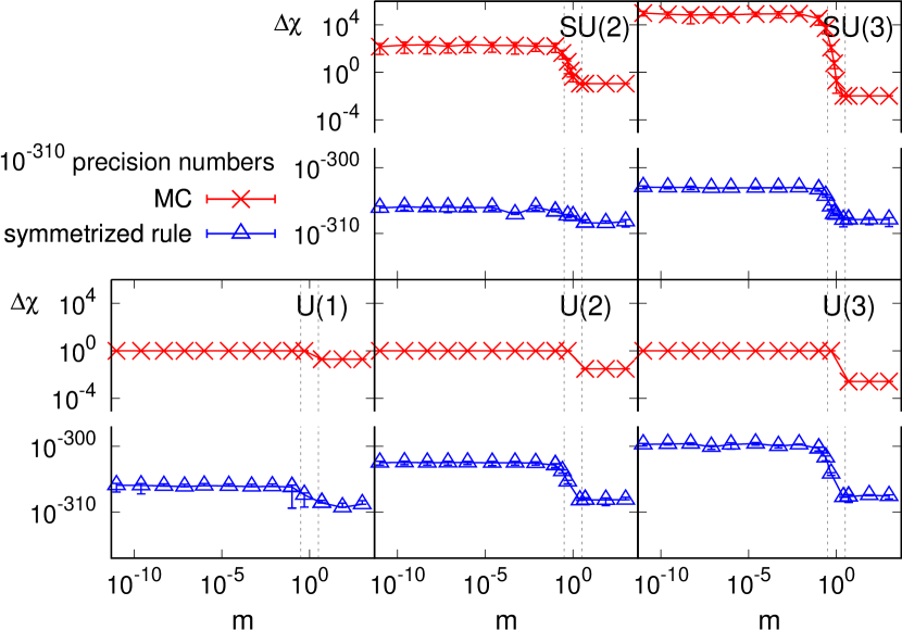
First, we describe the MC results: In the small $m$ region, $\Delta\chi$ for all groups are large - equal or larger than one. It can be shown that in this region the numerator of $\chi$ is such small that the MC evaluation cannot resolve these values for affordable sample sizes, resulting in large errors Volmer2018New . This is the manifestation of the sign-problem, making it almost impossible to compute reasonable values of $\chi$ with MC in the small $m$ region. On the other side, for large $m$ all groups have a smaller MC error estimate than in the small $m$ region. Here the numerator of $\chi$ tends to be larger and especially the denominator becomes very large, both resulting in a slightly better error estimate for the MC results.

Opposed to MC results, the symmetrized quadrature rules give error estimates approximately at machine precision up to very small $m$ values, see Figure 3. These numerical results show that the symmetrized quadrature rules give significant results in the sign-problem region in practice, where MC simulations have error estimates of order one.

3.2 Reducing high-dimensional integrals to nested one-dimensional integrals

The previous section shows efficient quadrature rules for physical one-dimensional integration to avoid the sign-problem. Most physical models have more than one integration variable. In general, it is not straightforward to find an efficient quadrature rule, and usually restricted Monte Carlo methods are applied to high-dimensional integrals. As a first alternative, we investigated the recursive numerical integration(RNI) method. This method reduces the $d$-dimensional integral

$$I(f)=\int_{D^{d}}f[\varphi]\,\text{d}\varphi$$ (22)

with $\text{d}\varphi=\prod_{i=1}^{d}\text{d}\varphi_{i}$ and $D=[0,2\pi)$ into many recursive one-dimensional integrals, and can be applied for several physical models of interest.

This is done by utilizing the typical structure of the integrand $f[\varphi]$. This section focuses on the RNI method and how to find an efficient quadrature rule for a high-dimensional integral. It does not discuss the sign-problem which is investigated further in section 3.3. More specifically, this section describes the two steps to create an efficient quadrature rules $Q(f)$ for the integral $I(f)$ in (22):

1. Use the structure of the integrand of the high-dimensional integral to rewrite it into recursive one-dimensional integrals.

2. Choose an efficient quadrature rule to compute each one-dimensional integral numerically. Recursively doing this results in the full quadrature rule $Q(f)$.

Finally, this section shows results of applying the method to a physical model called the topological osciallator. A more detailed explanation of the method and the results can be found in Ammon:2015mra ; Ammon:2016dfi .

RNI 1. Using the structure of the integrand

Many models in one physical dimensional have integrands with the structure

$$f[\varphi]=\prod_{i=1}^{d}f_{i}(\varphi_{i+1},\varphi_{i}),$$ (23)

with periodic boundary conditions $\varphi_{d+1}=\varphi_{1}$. These models have only next-neighbor couplings.

The integral of (23) can be rewritten using recursive integration as described in Genz86 ; Hayter06 : Because of next-neighbor couplings, each variable $\varphi_{i}$ appears only twice in $f[\varphi]$, in $f_{i}$ and $f_{i-1}$, and therefore the integral can be written as $d$ nested one-variable integrals $I_{i}$,

$$I(f)=\int_{D}...\int_{D}\prod_{i=1}^{d}f_{i}(\varphi_{i},\varphi_{i+1})\,\text{d}\varphi_{d}\cdots\text{d}\varphi_{1}$$ (24)

$$\leavevmode\resizebox{422.77661pt}{}{$\displaystyle{=\underbrace{\int_{D}\Bigg{(}...\underbrace{\bigg{(}\int_{D}f_{d-2}(\varphi_{d-2},\varphi_{d-1})\cdot\underbrace{\bigg{(}\int_{D}f_{d-1}(\varphi_{d-1},\varphi_{d})\cdot f_{d}(\varphi_{d},\varphi_{d+1})\,\text{d}\varphi_{d}\bigg{)}}_{I_{d}}\,\text{d}\varphi_{d-1}\bigg{)}}_{I_{d-1}}\cdots\Bigg{)}\,\text{d}\varphi_{1}}_{I_{1}}}$}.$$

This full integral can be computed recursively: $I_{d}$ integrates out $\varphi_{d}$ first, then $I_{d-1}$ integrates out $\varphi_{d-1}$ and so on until finally $I_{1}=I(f)$ integrates out $\varphi_{1}$.

To avoid under- and overflow of the single quadrature rule results, we actually used quadrature rules to approximate $I_{i}^{*}=\frac{1}{c_{i}}I_{i}$ with $c_{i}>0$ chosen adaptively. Then, the final integral is computed via $I=\left(\prod_{i=1}^{d}c_{i}\right)I^{*}$. For brevity, the method is described in the following without this trick.

Each integral is approximated by using an $N_{\text{quad}}$-point quadrature rule. The first integrand in (24) (last from the right) depends on three variables $\varphi_{d-1}$, $\varphi_{d}$ and $\varphi_{d+1}$. The variable $\varphi_{d}$ is integrated out, therefore the quadrature rule $Q_{d}(f_{d-1}\cdot f_{d})\equiv Q_{d}$ of $I_{d}$ depends on two variables,

$$Q_{d}(\varphi_{d-1},\varphi_{d+1})=\sum_{\gamma=1}^{N_{\text{quad}}}w_{\gamma}\,\,f_{d-1}(\varphi_{d-1},t_{\gamma})\,\,f_{d}(t_{\gamma},\varphi_{d+1}),$$ (25)

with sampling points $t$ and weights $w$. The next integral $I_{d-1}$ is approximated by the quadrature rule

$$Q_{d-1}(\varphi_{d-2},\varphi_{d+1})=\sum_{\gamma=1}^{N_{\text{quad}}}w_{\gamma}\,\,f_{d-2}(\varphi_{d-2},t_{\gamma})\,\,Q_{d}(t_{\gamma},\varphi_{d+1}),$$ (26)

and includes the quadrature rule $Q_{d}$ given in (25). The quadrature rules $Q_{d-2}$, …, $Q_{1}$ are created analogically to (26). Using the same sampling points $w_{\gamma}$ and weights $t_{\gamma}$, $\gamma\in\{1,...,N_{\text{quad}}\}$ in all quadrature rules $Q_{i}$ results in the full quadrature rule for (24),

$$Q=Q_{1}=\sum_{\gamma=1}^{N_{\text{quad}}}w_{\gamma}Q_{2}(t_{\gamma},t_{\gamma})=\text{tr}{\left[{{\prod_{i=1}^{d}\left(M_{i}\cdot\text{diag}{(w_{1},\dots,w_{N_{\text{quad}}})}\right)}}\right]},$$ (27)

with $M_{i}$ beeing an $N_{\text{quad}}\times N_{\text{quad}}$ matrix with entries $(M_{i})_{\alpha\beta}=f_{i}(t_{\alpha},t_{\beta})$.

RNI 2. Choosing an efficient quadrature rule

We used the Gaussian-Legendre $N_{\text{quad}}$-point quadrature rule, see stoer2013introduction to define the sampling points $t$ and weights $w$. For this rule, the error scales asymptotically (for large $N_{\text{quad}}$) as $\sigma\sim\mathcal{O}\left(\frac{1}{(2N_{\text{quad}})!}\right)$ (For Legendre polynomials the correct asymptotic error scaling is $\frac{(N_{\text{quad}}!)^{4}}{((2N_{\text{quad}})!)^{3}}$ kahaner1989numerical which is slightly improved over $\frac{1}{(2N_{\text{quad}})!}$.). The Stirling formula ($N_{\text{quad}}!\approx\sqrt{2\pi N_{\text{quad}}}\left(\frac{N_{\text{quad}}}{e}\right)^{N_{\text{quad}}}$ asymptotically) approximates the factorial to give

$$\sigma\sim\mathcal{O}\left(\exp(-2N_{\text{quad}}\ln N_{\text{quad}})\frac{1}{\sqrt{N_{\text{quad}}}}\right)$$ (28)

asymptotically. This is a huge improvement over the MC error scaling $1/\sqrt{N_{\text{MC}}}$.

Application to the topological oscillator

We applied the RNI method to the topological oscillator Bietenholz:2010xg , also called quantum rotor, which is a simple, physically one-dimensional model that has non-trivial characteristics which are also present in more complex models. It has $d$ variables $\phi_{i}\in[0,2\pi)$, a length scale $T$ and a coupling constant $c$. We investigated the topological charge susceptibility of this model,

$$\chi_{\text{top}} =\frac{\int O[\varphi]B[\varphi]\,\text{d}\varphi}{\int B[\varphi]\,\text{d}\varphi},$$ (29)

with Boltzmann-weight

$$B[\varphi] =\exp{\left(-c\sum_{i=1}^{d}\left(1-\cos(\varphi_{i+1}-\varphi_{i})\right)\right)},$$ (30)

and a squared topological charge

$$O[\varphi] =\frac{1}{T}\left(\frac{1}{2\pi}\sum_{i=1}^{d}(\varphi_{i+1}-\varphi_{i})\mod 2\pi\right)^{2}.$$ (31)

With RNI, we computed both numerator and denominator of $\chi_{\text{top}}$ separately, both differing in the factorization (23) of their integrands. Straightforwardly, the denominator integrand consists out of local exponential factors. The numerator consists out of summands with varying factorization schemes, each of these summands is computed separately with RNI and they are presented in more detail in Volmer2018New , section 5.2. We estimated the error of $\chi_{\text{top}}$ by choosing a large number of samples $N_{\text{quad}}^{g}$ in (25), (26) and similar ones for which we assumed that $\chi_{\text{top}}(N_{\text{quad}}^{g})$ has converged to the actual value and computed the difference of $\chi_{\text{top}}(N_{\text{quad}})$ for $N_{\text{quad}}<N_{\text{quad}}^{g}$ to this value,

$$\Delta\chi_{\text{top}}(N_{\text{quad}})=|\chi_{\text{top}}(N_{\text{quad}})-\chi_{\text{top}}(N_{\text{quad}}^{g})|.$$ (32)

We tested beforehand that this truncation error behaves exponentially for large $N_{\text{quad}}$ in practice, as expected from (28), Ammon:2015mra .

We compared the results of the RNI method with results using the Cluster algorithm Wolff:1988uh , which we found is an optimal MCMC method for the application to the topological oscillator Ammon:2015mra . Due to the exponential error scaling of the Gauss-Legendre rule, the new method advances MCMC for large enough $N_{\text{quad}}$. We found that the RNI method is also advantageous for lower $N_{\text{quad}}$-values: our simulations showed that the RNI method needs orders of magnitude less runtime than the Cluster algorithm to result in a specified error estimate on an observable, compare Figure 4 for $c=2.5$, $T=20$, $d=200$.

Figure 4: The runtime to arrive at a given error estimate is orders of magnitudes smaller when using the RNI method with Gauss-Legendre points than using the Cluster MCMC algorithm.

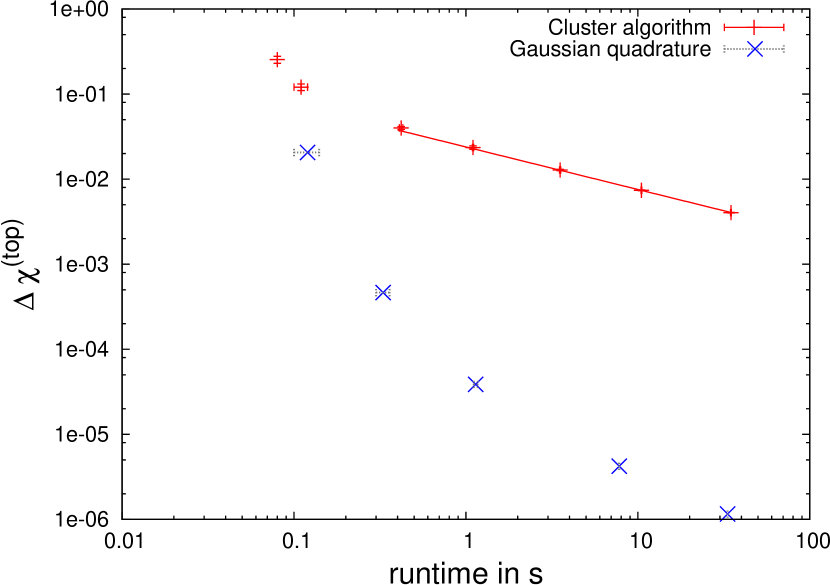
The Cluster algorithm measurements resulted in an error estimate that decreases proportional to $t^{-1/2}$ for runtime $t$, consistent with the typical MC error scaling probTheory . We used between $10^{2}$ and $10^{6}$ sampling points here. The RNI method, using between 10 and 300 sampling points with $N_{\text{quad}}^{g}=400$, resulted in orders of magnitude smaller errors. The exponential error scaling in (28) is not visible here, the asymptotic regime of the method is not yet reached with the used numbers of sampling points.

All in all, the RNI method results in orders of magnitude smaller errors than the Cluster algorithm for a fixed runtime or equivalently, the RNI method needs orders of magnitude less runtime than the Cluster algorithm to arrive at a fixed error estimate, even for a number of sampling points where the RNI error does not yet scale exponentially.

3.3 Avoiding the sign-problem in high-dimensional integrals

Section 3.1 shows that the sign-problem can be avoided for one-dimensional integrals using symmetric quadrature rules. But what about the sign-problem for high-dimensional integrals? A quadrature rule for high-dimensional integrals over compact groups,

$$I(f)=\int_{G^{d}}f[U]\,\text{d}U,$$ (33)

with $\text{d}U=\prod_{i=1}^{d}\text{d}U_{i}$ is needed that also avoids the sign-problem. We combined both already presented methods, the symmetric quadrature rules in section 3.1 and the RNI in section 3.2 to find an efficient quadrature rule $Q(f)$ for $I(f)$ in (33). An alternative attempt to generalize the symmetrized quadrature rules to high-dimensional integrals is discussed in 10.1007/978-3-319-75996-8_15 .

Combining recursive numerical integration and symmetric quadrature rules

RNI can be used to transform the high-dimensional integral $I(f)$ in (33) into one-dimensional integrals. These one-dimensional integrals can be approximated recursively, using the symmetric quadrature rules. In the following, these steps are described in more detail:

1. Find the structure, i.e. all $f_{i}$, of the integrand

   $$f[U]=\prod_{i=1}^{d}f_{i}(U_{i+1},U_{i}),$$ (34)

   to be able to write the full integral as nested one-dimensional integrals, similar to (24).

2. Apply symmetric quadrature rules to each one-dimensional integration over $U_{i}$. Here is an example how to do this for the innermost integral $I_{d}$, integrating over $U_{d}$:

   1. Rewrite the integral over $U_{d}$ into an integral over the products of spheres as done in (3.1).

   2. Approximate each iterated integral $I_{d}(g)$ by a product rule of quadratures over spheres parametrising the group $U_{d}$ to be integrated. Note that the group $U_{d}$ is parametrised at most as the product of $S^{1}$, $S^{3}$ and $S^{5}$.

Application to topological oscillator with sign-problem

We applied this combined method again to the topological oscillator discussed in 3.2. This time we transformed the variables $\varphi_{i}$ to new variables $U_{j}=\operatorname{\mathrm{e}}^{i\varphi_{j}}\in\mathcal{U}(1)$. Additionally, we added a sign-problem to the model by using an additional factor $\prod_{j=1}^{d}U_{j}^{-\theta}$ in the Boltzmann-weight,

$$B[U] =\exp{\left(-c\sum_{i=1}^{d}\Re(1-U_{i+1}U_{i}^{*})\right)}\cdot\prod_{j=1}^{d}U_{j}^{-\theta},$$ (35)

with a new parameter $\theta\in{\mathbb{R}}$. If this parameter is larger than zero, the sign-problem arises and is most severe for $\theta=\pi$.

In this model we computed the plaquette,

$$plaquette =\frac{\int O[U]B[U]\,\text{d}U}{\int B[U]\,\text{d}U},$$ (36)

with

$$O[U]=\frac{1}{d}\Re\left(\sum_{i=1}^{d}U_{i+1}U_{i}^{*}\right).$$ (37)

For the combined method, we computed both numerator and denominator of (36) separately and divided the values. We used a truncation error, similar to the one given in (32). We compared the method with a standard MC method as used in 3.1. The MC error is computed via the standard deviation.

For $\theta=\pi$ we found that the combined method avoids the sign-problem that is visible with the MC computation, compare Figure 5. It gives orders of magnitude smaller errors that shrink the more symmetrization points are used.

Figure 5: The combined method avoids the sign-problem that exists when using the MC method.

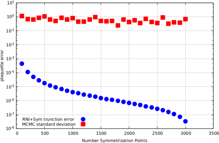
Therefore the combination of RNI and symmetric quadrature rules is suitable to avoid the sign-problem for high-dimensional integration.

4 Conclusion

In this contribution we have demonstrated that through symmetric quadrature rules exact symmetrization and recursive numerical integration techniques problems in high energy physics can be solved which constitute a major, if not unsurmountable obstacle for standard Markov chain Monte Carlo methods. The examples we have considered here invole only a time lattice and are hence 0+1-dimensional in space-time, where as real physical problem include spatials dimensions of up to 3. We are presently investigating whether the methods we have presented here can be extended to higher, i.e. including also spacial, dimensions. While for the recursive numerical integration technique we have first results which are promising, for the full symmetrization method we were so far not successful.

Also combining the symmetrized quadrature rules with MC methods did not lead to a practically feasible method in higher dimensions. However, we are following a path to combine Quasi Monte Carlo, recursive numerical integration and a full symmetrization to overcome this problem and hope to report about these attempts in the future.

References

- (1) Ammon, A., Genz, A., Hartung, T., Jansen, K., Leövey, H., Volmer, J.: Applying recursive numerical integration techniques for solving high dimensional integrals. PoS LATTICE2016, 335 (2016)
- (2) Ammon, A., Genz, A., Hartung, T., Jansen, K., Leövey, H., Volmer, J.: On the efficient numerical solution of lattice systems with low-order couplings. Comput. Phys. Commun. 198, 71–81 (2016). DOI 10.1016/j.cpc.2015.09.004
- (3) Ammon, A., Hartung, T., Jansen, K., Leövey, H., Volmer, J.: New polynomially exact integration rules on and . PoS LATTICE2016, 334 (2016)
- (4) Ammon, A., Hartung, T., Jansen, K., Leövey, H., Volmer, J.: New polynomially exact integration rules on U(N) and SU(N) (2016). URL https://inspirehep.net/record/1490030/files/arXiv:1610.01931.pdf
- (5) Ammon, A., Hartung, T., Jansen, K., Leövey, H., Volmer, J.: Overcoming the sign problem in one-dimensional QCD by new integration rules with polynomial exactness. Phys. Rev. D94(11), 114,508 (2016). DOI 10.1103/PhysRevD.94.114508
- (6) Bietenholz, W., Gerber, U., Pepe, M., Wiese, U.J.: Topological Lattice Actions. JHEP 1012, 020 (2010). DOI 10.1007/JHEP12(2010)020
- (7) Bilic, N., Demeterfi, K.: One-dimensional QCD With Finite Chemical Potential. Phys. Lett. B212, 83–87 (1988). DOI 10.1016/0370-2693(88)91240-3
- (8) Bloch, J., Bruckmann, F., Wettig, T.: Subset method for one-dimensional QCD. JHEP 10, 140 (2013). DOI 10.1007/JHEP10(2013)140
- (9) Bloch, J., Bruckmann, F., Wettig, T.: Sign problem and subsets in one-dimensional QCD. PoS LATTICE2013, 194 (2014)
- (10) Durr, S., et al.: Ab-Initio Determination of Light Hadron Masses. Science 322, 1224–1227 (2008). DOI 10.1126/science.1163233
- (11) Fristedt, B., Gray, L.: A Modern Approach to Probability Theory. Probability and Its Applications. Birkhäuser Basel (1997)
- (12) M. E. Peskin and D. V. Schroeder, An Introduction to quantum field theory.
- (13) Gattringer, C., Lang, C.B.: Quantum chromodynamics on the lattice. Lect. Notes Phys. 788, 1–343 (2010). DOI 10.1007/978-3-642-01850-3
- (14) T. DeGrand and C. E. Detar, Lattice methods for quantum chromodynamics New Jersey, USA: World Scientific (2006) 345 p
- (15) H. J. Rothe, Lattice gauge theories: An Introduction. World Sci. Lect. Notes Phys. 43 (1992) 1 [World Sci. Lect. Notes Phys. 59 (1997) 1] [World Sci. Lect. Notes Phys. 74 (2005) 1] [World Sci. Lect. Notes Phys. 82 (2012) 1].
- (16) Genz, A.: Fully Symmetric Interpolatory Rules for Multiple Integrals over Hyper-Spherical Surfaces. Journal of Computational and Applied Mathematics 157, 187–195 (2003). DOI 10.1016/S0377-0427(03)00413-8
- (17) Genz, A., Kahaner, D.K.: The numerical evaluation of certain multivariate normal integrals. J. Comput. Appl. Math. 16(2), 255–258 (1986). DOI 10.1016/0377-0427(86)90100-7. URL http://www.sciencedirect.com/science/article/pii/0377042786901007
- (18) Hartung, T., Jansen, K., Leövey, H., Volmer, J.: Improving monte carlo integration by symmetrization. In: A. Böttcher, D. Potts, P. Stollmann, D. Wenzel (eds.) The Diversity and Beauty of Applied Operator Theory, pp. 291–317. Springer International Publishing, Cham (2018)
- (19) Hayter, A.: Recursive integration methodologies with statistical applications. Journal of Statistical Planning and Inference 136(7), 2284–2296 (2006). DOI 10.1016/j.jspi.2005.08.024. URL http://www.sciencedirect.com/science/article/pii/S0378375805002223. In Memory of Dr. Shanti Swarup Gupta
- (20) Kahaner, D., Moler, C., Nash, S., Forsythe, G.: Numerical methods and software. Prentice-Hall series in computational mathematics. Prentice Hall (1989)
- (21) Stoer, J., Bartels, R., Gautschi, W., Bulirsch, R., Witzgall, C.: Introduction to Numerical Analysis. Texts in Applied Mathematics. Springer New York (2013)
- (22) Volmer, J.L.: New attempts for error reduction in lattice field theory calculations. Ph.D. thesis, Humboldt-Universität zu Berlin, Mathematisch-Naturwissenschaftliche Fakultät (2018). DOI http://dx.doi.org/10.18452/19350
- (23) Wolff, U.: Collective Monte Carlo Updating for Spin Systems. Phys. Rev. Lett. 62, 361 (1989). DOI 10.1103/PhysRevLett.62.361
- (24) T. Hartung and K. Jansen, Quantum computing of zeta-regularized vacuum expectation values arXiv:1808.06784 [quant-ph].
- (25) T. Hartung and K. Jansen, Integrating Gauge Fields in the -formulation of Feynman’s path integral arXiv:1902.09926 [math-ph].