Section 2

1 SIMPLE X-RAY SPECTRAL MODELLING OF DISK ABSORPTION IN IRAS 13224$-$3809

(Starting from the third paragraph)

Second, two photonionized-plasma absorption models xstar were constructed and fitted in XSPEC. The xstar models assume solar abundances except for that of iron and an ionizing luminosity of $10^{43}$ erg s^-1. A power law with $\Gamma=2$ is assumed for the ionizing spectrum. The redshift parameter ($z$) of the absorption models is fixed at the source redshift ($z=0.066$). Free parameters are the ionization of the plasma ($\xi^{\prime}$), the column density ($N_{\rm H}$), and the iron abundance ($Z_{\rm Fe}^{\prime}$, which is linked to that of the disk). Note that the solar abundances of xstar and relxillD are both taken from grevesse98.

Third, we calculate the relativistic effects of the orbiting absorbers at the surface of the disk by applying the same kdblur model to the two xstar models. The emissivity index ($q^{\prime}$) of the kdblur model is linked to the inner emissivity index parameter ($q_{1}$) of the relxillD model. The inner radius of the annular absorbers is fixed at 2 $r_{\rm g}$, and the outer radius of the annular absorbers is allowed to vary during our spectral fitting. The inclination angle ($i^{\prime}$) is linked to the disk inclination angle parameter ($i$) of relxillD. The total model is tbabs * ( (kdblur*xstar1) * (kdblur*xstar2) * relxillD + powerlaw) in the XSPEC format.

Table 1: Best-fit parameters for the low flux state and the high flux state spectra.

Model	Parameter	Unit	Low Flux	High Flux
kdblur	$R_{\rm out}$	$r_{\rm g}$	<11	<62
xstar1	$N_{\rm H,1}$	$10^{23}$cm-2	$7\pm 2$	$3\pm 2$
	$\log(\xi^{\prime}_{1})$	log(erg cm s-1)	$3.9^{+0.2}_{-0.3}$	$4.0\pm 0.4$
xstar2	$N_{\rm H,2}$	$10^{23}$cm-2	$4.5^{+2.1}_{-1.2}$	<1
	$\log(\xi^{\prime}_{2})$	log(erg cm s-1)	$3.4^{+0.3}_{-0.2}$	3.4 (fixed)
relxilld	$q_{1}$	-	$<2$	$4\pm 2$
	$q_{2}$	-	$>6$	$2^{+2}_{-1}$
	$R_{\rm break}$	$r_{\rm g}$	$6^{+3}_{-1}$	$<29$
	$i$	deg	$69^{+3}_{-2}$	$71^{+3}_{-2}$
	$\log(\xi)$	log(erg cm s-1)	$1.00\pm 0.05$	$1.03^{+0.08}_{-0.07}$
	$Z_{\rm Fe}$	$Z_{\odot}$	$2.8^{+1.2}_{-0.3}$	$2.9^{+2.1}_{-1.2}$
powerlaw	$\Gamma$	-	$2.77^{+0.06}_{-0.03}$	$2.99^{+0.06}_{-0.05}$
	$\chi^{2}$/$\nu$		111.43/109	126.34/118

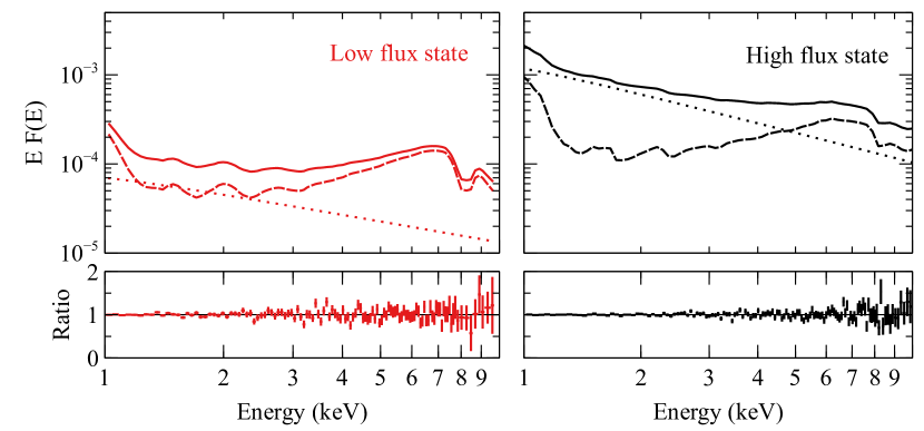
Figure 1: Left top: the best-fit model for the low flux state spectrum (red solid line). The red dashed line and the red dotted line show the absorbed disk reflection model and the power-law component respectively. Left bottom: the data/model ratio plot for the low flux state spectrum. Right: similar as the left panels but for the high flux state spectrum.

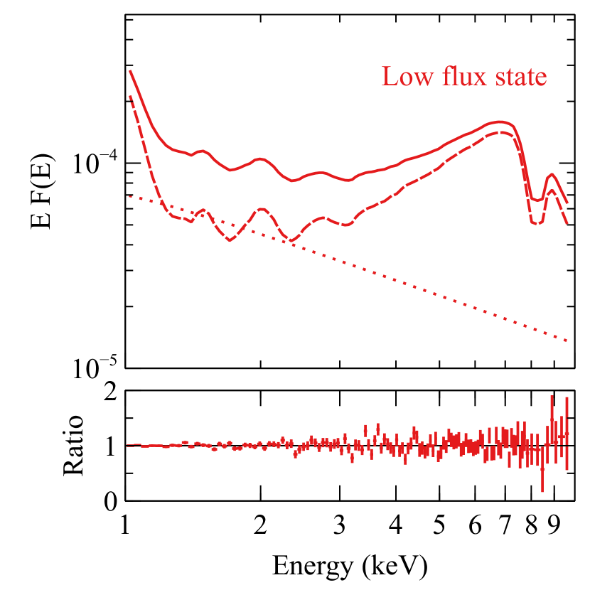
Figure 2: (Alternative plot of Fig. 1) Top: the best-fit model for the low flux state spectrum (red solid line). The red dashed line and the red dotted line show the absorbed disk reflection model and the power-law component respectively. Bottom: the data/model ratio plot for the low flux state spectrum.

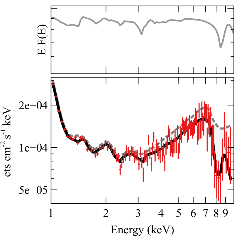
Figure 3: Top: the best-fit absorption model for the low flux state spectrum applied to a power law with $\Gamma=2$ to show the shape of the absorption lines. The normalization of the model is arbitrary in this figure. Bottom: the best-fit model for the low flux state spectrum (black). The unfolded low flux state spectrum is shown in red as reference. The dashed grey line shows the best-fit continuum model after removing absorption. The grey shaded region shows the model difference.

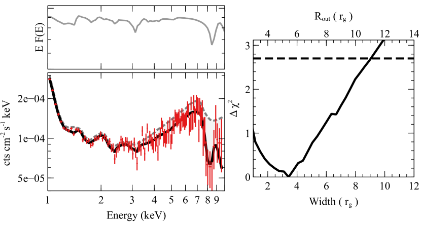
Figure 4: Alternative of Fig. 3 Top left: the best-fit absorption model for the low flux state spectrum applied to a power law with $\Gamma=2$ to show the shape of the absorption lines. The normalization of the model is arbitrary in this figure. Bottom left: the best-fit model for the low flux state spectrum (black). The unfolded low flux state spectrum is shown in red as reference. The dashed grey line shows the best-fit continuum model after removing absorption. The grey shaded region shows the model difference. Right: $\chi^{2}$ as a function of the maximum disk radius of the absorption zone. The inner radius of the annular absorber is fixed at 2 $r_{\rm g}$.

The best-fit models and the corresponding ratio plots can be found in Fig. 1, and the best-fit parameters are shown in Table 1. The models describe both the low flux state and the high flux state spectra very well.

For low flux state spectrum, the best-fit power-law continuum has a photon index of 2.77. The ionization of the disk reflection component is low with $\xi=10$ erg cm s^-1 and an iron abundance of $\approx 3$ compared to solar. A slightly higher disk viewing angle (69 deg) is obtained compared with previous fits [i.e. $i=67\pm 3$ deg obtained by fitting with reflionx][]jiang18. The best-fit emissivity profile shows a broad iron emission line with a stronger blue wing. A strong blue wing in the broad iron line profile is required to fit the spectrum to above 9 keV. This reflection component is exposed to the absorption model using the xstar models. The column density of the two absorbers ($N_{\rm H,1;2}=5-7\times 10^{23}$cm^-2) are much higher than values obtained by the outflow model [e.g. $N_{\rm H}\approx 10^{22}$cm^-2,][]jiang18. In order to better demonstrate how disk absorption works, we apply our best-fit absorption models to a power law with $\Gamma=2$ and show the model in the top panel of Fig. 3. The best-fit absorption model predicts very broad Fe xxv/xxvi, S xvi, and Si xiv absorption lines, which correspond to the line features at 8–9, 3.16, 2.42 keV in the real data. The red wing of the broad Fe xxv/xxvi absorption line extends to 6 keV, and affects the blue wing of the broad Fe K emission line in the reflection component. The shaded region in the bottom panel of Fig. 3 shows the difference between the unabsorbed and the absorbed models. The right panel of Fig.4 shows $\chi^{2}$ as a function of the maximum disk radius of the absorption zone. The best-fit outer radius of the absorbers is around $5.5$ $r_{\rm g}$, which suggests the absorbing zone is in the innermost region of the disk within a few $r_{\rm g}$.

(To Andy: Fig. 3 is an alternative plot of the original Fig. 1 in the draft. Feel free to use the old version if you think it is not necessary to show the absorption model.)

(To Andy: Fig. 4 is an alternative plot of Fig. 3. It combines the $\chi^{2}$ plot together with the model plot. It may save some space in your draft.)

(To Andy: if you do not wish to talk too much about the variability of the absorption but focus mainly on whether our model can fit the data or not, I think it is ok to shorten this paragraph and use Fig. 2 instead of Fig. 1.) For the high flux state spectrum, the best-fit power-law continuum has a softer photon index ($\Gamma=2.99$) compared with the low flux state spectrum. The ionization of the disk reflection component remains consistently low. The relativistic iron line shows a flatter emissivity profile. A lower column density of the first absorber is required for the first absorber, and a larger uncertainity of the ionization is found. By fixing the ionization of the second absorber at the best-fit value for the low flux state spectrum, we obtain an upper limit of the column density, suggesting weaker absorption in the high flux state. This result is consistent with previous work parker17,pinto18,jiang18. The outer radius of the absorption zone is less constrained (a 90% confidence range of $R_{\rm out}<$62 $r_{\rm g}$).

(To Andy: Shall we move this to Section 3? It is not so straightforward to calculate g-factor from the kdblur model. But the ray-tracing code calculates g-factor in different regions of the disk in more detail.) Using the relativistic Doppler formula and the measured value of Vsource we find g = Eobs/Eem ∼ 1.27 above the disk.