Asymptotics of Fredholm determinant associated with the Pearcey kernel
Abstract
The Pearcey kernel is a classical and universal kernel arising from random matrix theory, which describes the local statistics of eigenvalues when the limiting mean eigenvalue density exhibits a cusp-like singularity. It appears in a variety of statistical physics models beyond matrix models as well. We consider the Fredholm determinant of a trace class operator acting on with the Pearcey kernel. Based on a steepest descent analysis for a matrix-valued Riemann-Hilbert problem, we obtain asymptotics of the Fredholm determinant as , which is also interpreted as large gap asymptotics in the context of random matrix theory.
1 Introduction and statement of the results
In a series of papers [11]–[15], Brézin and Hikami initiated the studies of deformed complex Gaussian unitary ensemble (GUE) of the form
| (1.1) |
defined on the space of Hermitian matrices, where is a normalization constant and is a deterministic matrix also known as the external source. An interesting feature of this matrix ensemble is that it provides a simple model to create a phase transition for the eigenvalues of in the large limit. Indeed, by assuming the matrix is diagonal with two eigenvalues and of equal multiplicity, it follows from the work of Pastur [41] that if , the eigenvalues are distributed on two disjoint intervals, while for , the eigenvalues are distributed on a single interval. In the critical case when as , the gap closes at the origin and the limiting mean eigenvalue density exhibits a cusp-like singularity, i.e., the density vanishes like as . Upon letting and after proper scaling, a new local eigenvalue process characterized by the so-called Pearcey kernel emerges near the origin.
The Pearcey kernel is defined as (see [11, 12])
| (1.2) |
where ,
| (1.3) |
The contour in the definition of consists of the four rays , where the first and the third rays are oriented from infinity to zero while the second and the last rays are oriented outwards; see Figure 1 for an illustration. The functions and in (1.3) are solutions of the third order differential equations
| (1.4) | ||||
| (1.5) |
respectively. Since and were first introduced by Pearcey in the context of electromagnetic fields [42], the kernel bears the name Pearcey kernel. To see how describe the aforementioned phase transition, note that the eigenvalues of form a determinantal point process with a correlation kernel depending on (see [11, 12, 44]), it was established in [11, 12] (for ) and in [9, 43] (for general ) that
i.e., the correlation kernel converges to the Pearcey kernel near the origin as in a double scaling regime.
Like the classical kernels (sine kernel and Airy kernel) arising from random matrix theory [28, 37], the Pearcey kernel is a universal object as evidenced by its appearance in a variety of stochastic models. On one hand, the Pearcey statistics have been established in specific matrix models including large complex correlated Wishart matrices [31, 32], a two-matrix model with special quartic potential [30], and quite recently for general complex Hermitian Wigner-type matrices at the cusps [27], where the requirement on the identical distribution in Wigner matrices is dropped. It is worthwhile to mention that, for Wigner-type matrices, the density of states exhibits only square root or cubic root cusp singularities; see the classification theorem in [4, 5]. On the other hand, one also encounters the Pearcey kernel beyond matrix models, as can be seen from its connection with non-intersecting Brownian motions at cusps [2, 3, 9] and a combinatorial model on random partitions [39].
Let be the trace class operator acting on with the Pearcey kernel (1), it is well-known that the associated Fredholm determinant gives us the probability of finding no particles (also known as the gap probability) on the interval in a determinantal point process on the real line characterized by the Pearcey kernel. Moreover, it is shown in [3, 8, 11, 43] that the gap probability satisfies some nonlinear differential equations under more general settings. Since one cannot evaluate the Fredholm determinant explicitly for any fixed , a natural and fundamental question is then to ask for its large asymptotics, which will be the aim of the present work. Denote by
| (1.6) |
the logarithm of Fredholm determinant associated with the Pearcey kernel, our main result is the following theorem.
Theorem 1.1.
With defined in (1.6), we have, as ,
| (1.7) |
uniformly for in any compact subset of , where is an undetermined constant independent of and .
In the literature, the large asymptotics of was formally derived in [11] for , based on the coupled nonlinear differential equations satisfied by . Moreover, the asymptotics therein contains the leading term alone, without providing any information about the error estimate or the sub-leading terms. Our asymptotic expansion (1.7) includes more terms and improves the result in [11]. After a change of variable , the leading term of the asymptotic formula (1.7), i.e., , agrees with that obtained in [11, (3.36)]. Furthermore, we wish to emphasize that our derivation is rigorous, which makes use of integrable structure of the Pearcey kernel in the sense of Its-Izergin-Korepin-Slavnov [33] and involves a steepest descent analysis of the relevant Riemann-Hilbert (RH) problem. In a companion work [17], we also establish asymptotics of the deformed Pearcey determinant for , in the context of thinned Pearcey process, which exhibits significantly different behavior from that of the undeformed case presented in Theorem 1.1.
As also observed in [11], the leading term of the asymptotic formula (1.7) confirms the so-called Forrester-Chen-Eriksen-Tracy conjecture [16, 29]. This conjecture asserts that if the density of state behaves as near a point , then the probability of emptiness of the interval behaves like
| (1.8) |
In the present Pearcey case, we have and .
Evaluation of the constant in (1.7) is a challenging problem in the studies of large gap asymptotics [34]. For the classical sine, Airy and Bessel kernels encountered in random matrix theory, one could resolve this problem either by investigating the relevant Hankel or Toeplitz determinants which approximate the Fredholm determinants [19, 20, 22, 35], or by studying the total integrals of the Painlevé transcendents on account of Tracy-Widom type formulas for the gap probability [6]; see also [7, 25, 26] for the approach of operator theory. It seems unlikely that these methods are applicable in the present case. One rough idea to tackle this problem is based on the observation that, as the parameter tends to , the cusp singularity at the origin disappears and the origin becomes a regular point inside the bulk. Thus, we expect that might be related to the determinant of (generalized) sine kernel under certain scaling limits when , from which the constant term can be derived. We will leave this issue to a future publication.
Finally, we note that the asymptotics of Fredholm determinant associated with the Pearcey kernel is also investigated from the viewpoint of phase transition in [1, 8], i.e., to show how the Pearcey process becomes an Airy process by sending both and the parameter to positive infinity. We emphasize the asymptotic results therein are essentially different from ours.
The rest of this paper is devoted to the proof of Theorem 1.1. We mainly follow the general strategy established in [10, 21]. In Section 2, we relate the partial derivatives of to a RH problem with constant jumps, which is essential in the proof. After introducing some auxiliary functions defined on a Riemann surface with a specified sheet structure in Section 3, we then perform a Deift-Zhou steepest descent analysis [23] on this RH problem for large positive in Section 4. This asymptotic outcome, together with the differential identities for , will finally lead to the proof of Theorem 1.1, as presented in Section 5.
2 Differential identities for the Fredholm determinant
2.1 A Riemann-Hilbert characterization of the Pearcey kernel
The starting point toward the proof of Theorem 1.1 is an alternative representation of the Pearcey kernel via a RH problem, as shown in [9] and stated next.
RH problem 2.1.
We look for a matrix-valued function satisfying
-
(1)
Figure 2: The jump contours and the regions , , for the RH problem for . -
(2)
For , , the limiting values
exist, where the -side and -side of are the sides which lie on the left and right of , respectively, when traversing according to its orientation. These limiting values satisfy the jump relation
(2.2) where
(2.3) -
(3)
As and , we have
(2.4) where
(2.5) with
(2.6) , and
(2.7) Moreover, are constant matrices
(2.8) with , and is given by
(2.9) with
(2.10) -
(4)
is bounded near the origin.
It is shown in [9, Section 8.1] that the above RH problem has a unique solution expressed in terms of solutions of the Pearcey differential equation (1.4). Indeed, note that (1.4) admits the following solutions:
| (2.11) |
where
We then have
| (2.12) |
where , , is the region bounded by the rays and (with ); see Figure 1 for an illustration.
Remark 2.2.
For our purpose, we present a refined asymptotics of at infinity in (2.4), which can be verified directly from (2.12). To see this, let us focus on the case , since the asymptotics in other regions can be derived in a similar way. Carrying out a steepest descent analysis to the integrals defined (2.11) (cf. [9, 38]), we have, as ,
| (2.13) |
| (2.14) |
for and
| (2.15) |
for where , , are given in (2.10), and are polynomials in given in (2.6) and (2.7). The asymptotic expansions of and , , can be derived in a similar fashion or simply by taking derivatives on the right hand sides of (2.13)–(2.15). A combination of all these asymptotic results and (2.12) then gives us (2.4) after a straightforward calculation.
2.2 Differential equations for
For later use, we need the following linear differential equations for with respect to and .
Proposition 2.3.
2.3 Differential identities for
With the function defined in (1.6), we have
| (2.25) |
where stands for the kernel of the resolvent operator, that is,
Since the kernel of the operator is integrable in the sense of [33], its resolvent kernel is integrable as well; cf. [21, 33]. Indeed, by setting
| (2.26) |
we have
| (2.27) |
We could also represent in terms of and defined in (2.26). To proceed, we note from (2.24) and (2.19) that
| (2.28) |
Moreover, by taking derivative with respect to on both sides of , it is readily seen from (2.19) that
| (2.29) |
which gives us
| (2.30) |
This, together with (2.23) and (2.28), implies
| (2.31) |
Hence, we obtain
| (2.32) |
We next establish the connection between the functions , and an RH problem with constant jumps, which is based on the fact that the resolvent kernel is related to the following RH problem.
RH problem 2.4.
We look for a matrix-valued function satisfying the following properties:
-
(1)
is defined and analytic in , where the orientation is taken from the left to the right.
- (2)
-
(3)
As ,
(2.34) -
(4)
As , we have .
Recall the RH problem 2.1 for , we make the following undressing transformation to arrive at an RH problem with constant jumps. To proceed, the four rays , , emanating from the origin are replaced by their parallel lines emanating from some special points on the real line. More precisely, we replace and by their parallel rays and emanating from the point , replace and by their parallel rays and emanating from the point . Furthermore, these rays, together with the real axis, divide the complex plane into six regions I-VI, as illustrated in Figure 3.
Proposition 2.5.
Proof.
We only need to show that does not have a jump over , while the other claims follow directly from (2.40) and the RH problem 2.1 for .
By (2.24), we have, for ,
| (2.46) |
This, together with (2.33) and (2.40), implies that for ,
| (2.47) |
as desired.
This completes the proof of Proposition 2.5. ∎
The connections between the above RH problem and the partial derivatives of are revealed in the following proposition.
Proposition 2.6.
Proof.
We begin with the proof of (2.48). From (2.34) and (2.35), it follows that
| (2.50) |
This, together with (2.32), implies that
| (2.51) |
By (2.45), it is readily seen that . With the aid of the explicit expressions of and in (2.5), we then have , which gives us (2.48) in view of (2.51).
We next consider . For , we see from (2.24), (2.36) and (2.40) that
| (2.52) |
and
| (2.53) |
Combining the above formulas, (2.25), (2.27) and L’Hôspital’s rule then gives us
| (2.54) |
where the above limits are taken from the region II. Similarly, one can show that (2.54) also holds provided the limits are taken from the region V.
The expression (2.54) can be further simplified via the following symmetric relation of :
| (2.55) |
where
| (2.56) |
is a nonsingular matrix with given in (2.5), and
| (2.57) |
To see (2.55), let us consider the function
| (2.58) |
It is straightforward to check that satisfies the same jump condition as shown in (2.42) and (2.43). This means is analytic in the complex plane with possible isolated singular points located at . Since as , we conclude that the possible singular points are removable. In view of the asymptotics of given in (2.44), we further obtain from (2.58) and a bit more cumbersome calculation that
with given in (2.56). An appeal to Liouville’s theorem then leads us to (2.55).
As a consequence of (2.55), we have
This, together with (2.55) and the fact that , implies
To this end, we observe that for an arbitrary matrix ,
A combination of the above two formulas shows that
This completes the proof of Proposition 2.6. ∎
3 Auxiliary functions
In this section, we introduce some auxiliary functions and study their properties. The aim is to construct the so-called -functions, of which the analytic continuation defines a meromorphic function on a Riemann surface with a specified sheet structure. The -functions have desired behavior around each branch point, and will be crucial in our further asymptotic analysis of the RH problem 2.5 for .
Throughout this section, unless specified differently, we shall take the principal branch for all fractional powers.
3.1 A three-sheeted Riemann surface and the -functions
We introduce a three-sheeted Riemann surface with sheets
We connect the sheets , , to each other in the usual crosswise manner along the cuts and . More precisely, is connected to along the cut and is connected to along the cut . We then compactify the resulting surface by adding a common point at to the sheets and , and a common point at to the sheets and . We denote this compact Riemann surface by , which has genus zero and is shown in Figure 4.
We intend to find functions , , on these sheets, such that each is analytic on and admits an analytic continuation across the cuts. For this purpose, we start with an elementary function that is meromorphic on , which satisfies the following algebraic equation
| (3.1) |
We choose three solutions , , to (3.1) such that they are defined and analytic on , respectively. Each function maps to certain domain in the extended complex -plane . The correspondences between some points and the points are given in Table 1, where denotes the point on the closure of the -th sheet .
| 1 | 0 |
Due to the sheet structure shown in Figure 4, it follows that , and . Moreover, we actually have the following explicit expressions for .
Proposition 3.1.
Proof.
Clearly, and satisfies the quadratic equation
| (3.5) |
Hence, with , , defined in (3.2), we have
as expected, where in the last step we have made use of (3.5). Furthermore, an elementary analysis shows that for . Thus, and . This, together with (3.2), implies that , , and . The other relations in Table 1 can then be verified similarly, and we omit the details here.
This completes the proof of Proposition 3.1. ∎
As a consequence of Proposition 3.1, we have the following properties of .
Proposition 3.2.
The functions , , given in (3.2) satisfy the following properties.
-
(a)
is analytic on , , and
(3.6) (3.7) Here, we orient and from the left to the right. Hence, the function has an analytic continuation to a meromorphic function . This function is a bijection.
-
(b)
satisfies the symmetry properties
(3.8) (3.9) (3.10) -
(c)
As and , we have
(3.11) and
(3.12) -
(d)
As and , we have
(3.13) and
(3.14) -
(e)
As and , we have
(3.15) and
(3.16)
Proof.
While (3.8) follows directly from (3.2), the proof of (3.9) relies on the fact that
Hence, by (3.2), it follows that
which is (3.9). The relation (3.10) follows in a similar manner.
To obtain the asymptotics of , , as , we observe from the definition of in (3.3) that
Inserting the above formula into (3.2), it is readily seen that, if and ,
which is the first formula in (3.11). This, together with the fact that , implies the second formula of (3.11). The asymptotics of in (3.12) can be derived through similar computations, we omit the details here.
We next come to the asymptotics of , , as . Since
it follows from (3.3) that
with . A combination of the above formula and (3.2) then gives us
as shown in (3.13). The asymptotics of in (3.13) can be proved in a similar manner, we omit the details here.
Finally, we note that, as ,
with . Inserting the above formula into (3.2) then gives us (3.15) and (3.16) after straightforward calculations.
This completes the proof of Proposition 3.2. ∎
The image of the map is illustrated in Figure 5.
3.2 The -functions
With the functions given in Proposition 3.1, we define the -functions as
| (3.18) |
which depend on the parameters and . The properties of the -functions are listed in the following proposition.
Proposition 3.3.
The functions , , defined by (3.18) have the following properties.
-
(a)
is analytic on , , and
(3.19) (3.20) Hence the function has an analytic continuation to a meromorphic function on the Riemann surface .
-
(b)
We have the following symmetry properties
(3.21) (3.22) (3.23) -
(c)
As and , we have
(3.24) and
(3.25) where
(3.26) -
(d)
As and , we have
(3.27) and
(3.28) where
(3.29) - (e)
-
(f)
For , we have
(3.32)
Proof.
The proofs of items (a)–(e) follow directly from the definition of in (3.18) and Proposition 3.2. It then remains to prove (3.32). Since , , are three solutions of the algebraic equation (3.1), it follows from Vieta’s rule that, for ,
Hence,
| (3.33) |
and
| (3.34) |
This completes the proof of Proposition 3.3. ∎
4 Asymptotic analysis of the Riemann-Hilbert problem for
In this section, we shall perform a Deift-Zhou steepest descent analysis [23] to the RH problem for as . It consists of a series of explicit and invertible transformations which leads to an RH problem tending to the identity matrix as .
4.1 First transformation:
This transformation is a rescaling of the RH problem for , which is defined by
| (4.1) |
It is then straightforward to check that satisfies the following RH problem.
4.2 Second transformation:
In this transformation we normalize the large behavior of using the -functions introduced in Section 3.2. We define
| (4.7) |
where
| (4.8) |
with and being the constants given in (3.26), and the functions , , are defined in (3.18). Then, satisfies the following RH problem.
Proposition 4.2.
Proof.
By (4.7), it is clear that is defined and analytic in and
| (4.13) |
for , where is given in (4.3). This, together with item (a) in Proposition 3.3, gives us (4.10).
Checking the asymptotics (4.11) is a bit more cumbersome. To that end, we observe from Proposition 3.3 and (4.6) that the following formula is useful
We omit the details here.
This completes the proof of Proposition 4.2. ∎
4.3 Estimate of for large
The jump matrix defined in (4.10) is constant on and on . On the other jump contours, it comes out that the nonzero off-diagonal entries of are all exponentially small for large , which can be seen from the following proposition. In what follows, we denote by the fixed open disk centered at with small radius .
Proposition 4.3.
-
(a)
There exist positive constants such that
(4.14) (4.15) for large enough.
-
(b)
There exists a constant such that
(4.16) (4.17) for large enough.
Proof.
We will only present the proof of (4.14), since the proofs of other estimates are analogous. In view of the symmetry properties (3.21), it suffices to show (4.14) for . To this end, let us define
| (4.18) |
From the behavior of the -functions at infinity given in Proposition 3.3, it follows from an elementary analysis that
| (4.19) |
for some , if is large enough. This, together with the triangle inequality, implies that it is sufficient to show (4.14) for , .
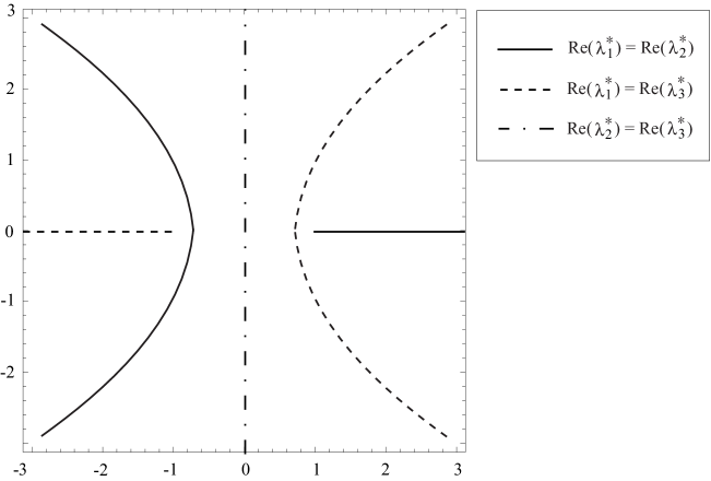
For large value of , the estimate follows from the asymptotics of at infinity, which can be obtained by taking in item (c) of Proposition 3.3. For bounded , the claim is supported by Figure 6. The sign of remains unchanged in the region bounded by the solid lines in Figure 6. By using the asymptotics of and at infinity, it is readily seen that for all on the right side of the solid curve excluding , which particularly holds for the finite part of .
This completes the proof of Proposition 4.3. ∎
As a consequence of the above proposition, the following corollary about the estimate of is immediate.
Corollary 4.4.
There is a constant such that
uniformly for .
4.4 Global parametrix
By Corollary 4.4, if we suppress all entries of the jump matrices for that decay exponentially as , we are led to the following RH problem for the global parametrix .
RH problem 4.5.
We look for a matrix-valued function satisfying
-
(1)
is defined and analytic in .
-
(2)
satisfies the jump condition
(4.20) - (3)
The above RH problem can be solved explicitly. Let the scalar functions , be defined as
| (4.22) |
where the branch cut for the square root is taken along , i.e., the curve defined by ; see Figure 5 for an illustration. It is shown in [24, Section 6.1.5] that the solution to RH problem 4.5 is given by
| (4.23) |
where is defined in (2.57) and
| (4.24) |
is an invertible constant matrix.
It is worthwhile to mention that satisfies the following symmetric relation (see [24, Equations (2.2.30) and (6.1.38)])
| (4.25) |
or equivalently,
| (4.26) |
where
| (4.27) |
Finally, from the asymptotic behaviors of the -functions given in Proposition 3.2, it is readily seen that the following proposition regarding the refined asymptotic behaviors of the global parametrix near and .
4.5 Local parametrix near
Due to the fact that the convergence of the jump matrices to the identity matrices on and is not uniform near , we intend to find a function satisfying an RH problem as follows.
RH problem 4.7.
We look for a matrix-valued function satisfying
-
(1)
is defined and analytic in .
- (2)
-
(3)
As , matches on the boundary of , i.e.,
(4.32)
The RH problem 4.7 for can be solved explicitly with the aid of the Bessel parametrix described in Appendix A. To this aim, we introduce the local conformal mapping
| (4.33) |
By (3.27) and (3.28), we have that is analytic in and, as ,
| (4.34) |
with the constants and given in (3.29). Let be the Bessel parametrix in (A.1) with , we set, for ,
| (4.37) |
where is defined in (4.33) and
| (4.38) |
with given in (4.23).
Proof.
From (A.2), it is straightforward to check that satisfies the jump condition in (4.31) provided the prefactor is analytic in . To see this, we note that the only possible jump for is on the interval . For , it is readily seen from (4.34) that . Hence, we obtain from the jump of in (4.20) that
This shows that is indeed analytic in .
It remains to verify the matching condition (4.32). From the local behaviors of and near given in item (d) of Proposition 3.3, the function appearing in the last term of (4.5) is exponentially small as for . Thus, it follows from the asymptotic behavior of the Bessel parametrix at infinity in (A.3) that, for ,
| (4.39) |
where
| (4.40) |
which gives us (4.32).
This completes the proof of Proposition 4.8. ∎
We conclude this section by evaluating and for later use. The calculations are straightforward and cumbersome by combining (4.38) and the asymptotics of and given in (4.28) and (4.34). We omit the details but present the results below.
| (4.41) |
and
| (4.42) |
where the constants and are given in (3.29), and stands for some unimportant entry.
4.6 Local parametrix near
Similar to the situation encountered near , we intend to find a function satisfying the following RH problem near .
RH problem 4.9.
We look for a matrix-valued function satisfying
-
(1)
is defined and analytic in .
- (2)
-
(3)
As , we have
(4.44)
Again, the RH problem 4.9 can be solved with the help of the Bessel parametrix , following the same spirit in the construction of . The conformal mapping now reads
| (4.45) |
From (3.22) and (3.23), one can see that
| (4.46) |
where is defined in (4.33). In view of (4.34), this also implies that, as ,
| (4.47) |
with the constants and given in (3.29). For , we then set
| (4.50) |
where is defined in (4.45) and
| (4.51) |
It comes out that is closely related to . To see the relation, we observe from (4.26) and (4.46) that
| (4.52) |
where the constant matrices and are given in (2.57) and (4.27), respectively. A further appeal to the symmetric relations (3.22) and (3.23) then implies
| (4.53) |
This in turn shows that the fulfills the jump condition (4.43) and the matching condition (4.44). In particular, we have, as ,
| (4.54) |
where
| (4.55) |
Again, using (4.26) and (4.46), it is readily seen from (4.40) that
| (4.56) |
where we have made use of the fact that ; see (4.27). In summary, we have proved the following proposition.
4.7 Final transformation
Our final transformation is defined by
| (4.57) |
It is then easily seen that satisfies the following RH problem.
RH problem 4.11.
In view of Corollary 4.4, it follows that the jumps of tend to the identity matrix exponentially fast as , except for those on ; see also (4.39) and (4.54) for the expansions of on and . Then, by a standard argument (cf. [18]), we conclude that, as ,
| (4.61) |
uniformly for . Moreover, a combination of (4.61) and RH problem 4.11 shows that solves the following RH problem.
RH problem 4.12.
By Cauchy’s residue theorem, the solution to the above RH problem is given by
| (4.63) |
For our purpose, we need to know the exact value of . From the local behaviors of and near given in (4.28) and (4.34), we obtain from (4.40) that
| (4.64) |
where
| (4.65) |
with given in (3.29). Although the explicit formulas of and in (4.7) are also available and is indeed involved in our later calculation, we decide not to include the exact formulas here due to their complicated forms. Also note that (see (4.6)), it is then readily seen that
| (4.66) |
Hence, in view of (4.63), we arrive at
| (4.67) |
where is given in (4.7).
We are now ready to prove Theorem 1.1.
5 Proof of Theorem 1.1
Our strategy is to find the large asymptotics of and by making use of the differential identities established in Proposition 2.6, which will in turn give us the asymptotics of .
We start with deriving the asymptotics of . Substituting (4.1) into the differential identity (2.49) gives us
| (5.1) |
where ′ denotes the derivative with respect to . Tracing back the invertible transformations and in (4.7) and (4.57), it follows that
| (5.2) |
In addition, from the explicit expression of in (4.5), we further obtain
| (5.3) |
for and , where
| (5.4) |
and
| (5.5) |
Since the prefactor in (5.3) is independent of , we have
| (5.6) |
We next evaluate the four terms on the right hand side of the above formula one by one. For the first term in (5.6), we see from (5.4) that
| (5.7) |
Thus,
| (5.8) |
For the second term in (5.6), we recall the following properties of the modified Bessel functions (cf. [40, Chapter 10]):
where is the Euler’s constant. This, together with (5.5) and (A.1), implies that, as ,
| (5.9) |
and
| (5.10) |
A combination of these two formulas shows
| (5.11) |
To this end, we note that for an arbitrary matrix , it is readily seen from (5.4) that
| (5.12) |
We then obtain from (5.11), (5.12) and the facts (see (4.34)) that
| (5.13) | ||||
| (5.14) |
where is given in (3.29).
Regrading the last two terms in (5.6), we first observe from items (d) and (f) of Proposition 3.3 that
| (5.15) |
This means the exponential terms on the right hand side of (5.12) are exponentially small as for in any compact subset of . Next, it is readily seen from (5.9), (5.10) and (4.34) that, for an arbitrary matrix ,
| (5.16) |
This, together with (5.12) and (5.15), implies that
| (5.17) | |||
for an arbitrary small constant , i.e., the above two terms are exponentially small as . Similarly, we also have
| (5.18) |
| (5.19) |
For the limit of the right hand side on of (5.18), it follows from the explicit expressions of and given in (4.41) and (4.42) that
| (5.20) |
For the limit of the right hand side on of (5.19), we note from (4.61) that, as ,
| (5.21) |
In view of the explicit expressions of and in (4.41) and (4.67), it is then readily seen that
| (5.22) |
where the constants , , are given in (3.29).
Finally, by (5.1), (5.6), (5.8), (5.13), (5.18), (5.19), (5.20) and (5.22), we obtain
| (5.23) |
as . Integrating the above formula gives us
| (5.24) |
uniformly for in any compact subset of , where is the constant of integration that might be dependent on .
To find more information about , we come to . From (2.48) and (4.12), we have
| (5.25) |
where and are given in (4.12) and (3.26), respectively. Recall that (see (4.57))
it follows from the large behaviors of , and in (4.11), (4.29) and (4.68) that
| (5.26) |
where and are the coefficients of for and at infinity. A combination of the above formula and the expressions of and in (4.30) and (4.7) gives us
| (5.27) |
This, together with (5.25) and given in (3.26), further implies
| (5.28) |
Comparing this approximation with the asymptotics of given in (5.24), it is easily seen that
| (5.29) |
where is an undetermined constant independent of and . Inserting (5.29) into (5.24) leads to our final asymptotic result (1.7).
This completes the proof of Theorem 1.1. ∎
Appendix A Bessel parametrix
Define
| (A.1) |
where and denote the modified Bessel functions (cf. [40, Chapter 10]), the principle branch is taken for and the regions I-III are illustrated in Fig. 8. By [36], we have that satisfies the RH problem below.
RH problem for
-
(a) is defined and analytic in , where the contours , , are indicated in Figure 8.
-
(b) satisfies the jump condition
(A.2) -
(c) satisfies the following asymptotic behavior at infinity:
(A.3) -
(d) satisfies the following asymptotic behaviors near the origin:
If ,(A.4) If ,
(A.5) If ,
(A.6)
Acknowledgements
Dan Dai was partially supported by a grant from the City University of Hong Kong (Project No. 7005252), and grants from the Research Grants Council of the Hong Kong Special Administrative Region, China (Project No. CityU 11303016, CityU 11300520). Shuai-Xia Xu was partially supported by National Natural Science Foundation of China under grant numbers 11971492, 11571376 and 11201493. Lun Zhang was partially supported by National Natural Science Foundation of China under grant numbers 11822104 and 11501120, by The Program for Professor of Special Appointment (Eastern Scholar) at Shanghai Institutions of Higher Learning, and by Grant EZH1411513 from Fudan University. He also thanks Marco Bertola for helpful discussions related to this work.
References
- [1] M. Adler, M. Cafasso and P. van Moerbeke, From the Pearcey to the Airy process, Electron. J. Probab. 16 (2011), 1048–1064.
- [2] M. Adler, N. Orantin and P. van Moerbeke, Universality for the Pearcey process, Phys. D 239 (2010), 924–941.
- [3] M. Adler and P. van Moerbeke, PDEs for the Gaussian ensemble with external source and the Pearcey distribution, Comm. Pure Appl. Math. 60 (2007), 1261–1292.
- [4] O. H. Ajanki, L. Erdős and T. Krüger, Singularities of solutions to quadratic vector equations on the complex upper half-plane, Comm. Pure Appl. Math. 70 (2017), 1672–1705.
- [5] J. Alt, L. Erdős and T. Krüger, The Dyson equation with linear self-energy: spectral bands, edges and cusps, Doc. Math. 25 (2020), 1421–1539.
- [6] J. Baik, R. Buckingham and J. DiFranco, Asymptotics of Tracy-Widom distributions and the total integral of a Painlevé II function, Comm. Math. Phys. 280 (2008), 463–497.
- [7] E. L. Basor and T. Ehrhardt, On the asymptotics of certain Wiener-Hopf-plus-Hankel determinants, New York J. Math. 11 (2005), 171–203.
- [8] M. Bertola and M. Cafasso, The transition between the gap probabilities from the Pearcey to the Airy process–a Riemann-Hilbert approach, Int. Math. Res. Not. IMRN 2012 (2012), 1519–1568.
- [9] P. M. Bleher and A. B. J. Kuijlaars, Large limit of Gaussian random matrices with external source, part III: double scaling limit, Comm. Math. Phys. 270 (2007), 481–517.
- [10] A. Borodin and P. Deift, Fredholm determinants, Jimbo-Miwa-Ueno -functions, and representation theory, Comm. Pure Appl. Math. 55 (2002), 1160–1230.
- [11] E. Brézin and S. Hikami, Level spacing of random matrices in an external source, Phys. Rev. E. 58 (1998), 7176–7185.
- [12] E. Brézin and S. Hikami, Universal singularity at the closure of a gap in a random matrix theory, Phys. Rev. E. 57 (1998), 4140–4149.
- [13] E. Brézin and S. Hikami, Extension of level-spacing universality, Phys. Rev. E 56 (1997), 264–269.
- [14] E. Brézin and S. Hikami, Spectral form factor in a random matrix theory, Phys. Rev. E 55 (1997), 4067–4083.
- [15] E. Brézin and S. Hikami, Correlations of nearby levels induced by a random potential, Nucl. Phys. B 479 (1996), 697–706.
- [16] Y. Chen, K. Eriksen and C. A. Tracy, Largest eigenvalue distribution in the double scaling limit of matrix models: a Coulomb fluid approach, J. Phys. A 28 (1995), L207–L211.
- [17] D. Dai, S.-X. Xu and L. Zhang, On the deformed Pearcey determinant, arXiv:2007.12691.
- [18] P. Deift, Orthogonal Polynomials and Random Matrices: A Riemann-Hilbert Approach, Courant Lecture Notes 3, New York University, 1999.
- [19] P. Deift, A. Its and I. Krasovsky, Asymptotics of the Airy-kernel determinant, Comm. Math. Phys. 278 (2008), 643–678.
- [20] P. Deift, A. Its, I. Krasovsky and X. Zhou, The Widom-Dyson constant for the gap probability in random matrix theory, J. Comput. Appl. Math. 202 (2007), 26–47.
- [21] P. Deift, A. Its and X. Zhou, A Riemann-Hilbert approach to asymptotic problems arising in the theory of random matrix models, and also in the theory of integrable statistical mechanics, Ann. of Math. (2) 146 (1997), 149–235.
- [22] P. Deift, I. Krasovsky and J. Vasilevska, Asymptotics for a determinant with a confluent hypergeometric kernel, Int. Math. Res. Not. IMRN 2011 (2011), 2117–2160.
- [23] P. Deift and X. Zhou, A steepest descent method for oscillatory Riemann-Hilbert problems. Asymptotics for the MKdV equation, Ann. of Math. (2) 137 (1993), 295–368.
- [24] K. Deschout, Multiple orthogonal polynomial ensembles, Ph.D. Thesis, KU Leuven, 2012.
- [25] T. Ehrhardt, The asymptotics of a Bessel-kernel determinant which arises in random matrix theory, Adv. Math. 225 (2010), 3088–3133.
- [26] T. Ehrhardt, Dyson’s constant in the asymptotics of the Fredholm determinant of the sine kernel, Comm. Math. Phys. 262 (2006), 317–341.
- [27] L. Erdős, T. Krüger and D. Schröder, Cusp universality for random matrices I: local Law and the complex Hermitian case, Comm. Math. Phys. 378 (2020), 1203–1278.
- [28] P. J. Forrester, Log-gases and Random Matrices, London Mathematical Society Monographs Series, 34., Princeton University Press, Princeton, NJ, 2010.
- [29] P. J. Forrester, The spectrum edge of random matrix ensembles, Nucl. Phys. B 402 (1993), 709–728.
- [30] D. Geudens and L. Zhang, Transitions between critical kernels: from the tacnode kernel and critical kernel in the two-matrix model to the Pearcey kernel, Int. Math. Res. Not. IMRN 2015 (2015), 5733–5782.
- [31] W. Hachem, A. Hardy and J. Najim, Large complex correlated Wishart matrices: fluctuations and asymptotic independence at the edges, Ann. Probab. 44 (2016), 2264–2348.
- [32] W. Hachem, A. Hardy and J. Najim, Large complex correlated Wishart matrices: the Pearcey kernel and expansion at the hard edge, Electron. J. Probab. 21 (2016), Paper No. 1, 36 pp.
- [33] A. R. Its, A. G. Izergin, V. E. Korepin and N. A. Slavnov, Differential equations for quantum correlation functions, Internat. J. Modern Phys. B 4 (1990), 1003–1037.
- [34] I. Krasovsky, Large Gap Asymptotics for Random Matrices, XVth International Congress on Mathematical Physics, New Trends in Mathematical Physics, Springer, 2009, 413–419.
- [35] I. Krasovsky, Gap probability in the spectrum of random matrices and asymptotics of polynomials orthogonal on an arc of the unit circle, Int. Math. Res. Not. IMRN 2004 (2004), 1249–1272.
- [36] A. B. J. Kuijlaars, K. T-R. McLaughlin, W. Van Assche and M. Vanlessen, The Riemann-Hilbert approach to strong asymptotics for orthogonal polynomials on , Adv. Math. 188 (2004), 337–398.
- [37] M. L. Mehta, Random Matrices, 3rd ed., Elsevier/Academic Press, Amsterdam, 2004.
- [38] T. Miyamoto, On an Airy function of two variables, Nonlinear Anal. 54 (2003), 755–772.
- [39] A. Okounkov and N. Reshetikhin, Random skew plane partitions and the Pearcey process, Comm. Math. Phys. 269 (2007), 571–609.
- [40] F. W. J. Olver, A. B. Olde Daalhuis, D. W. Lozier, B. I. Schneider, R. F. Boisvert, C. W. Clark, B. R. Miller and B. V. Saunders, eds, NIST Digital Library of Mathematical Functions, http://dlmf.nist.gov/, Release 1.0.21 of 2018-12-15.
- [41] L. A. Pastur, The spectrum of random matrices, Teoret. Mat. Fiz. 10 (1972), 102–112.
- [42] T. Pearcey, The structure of an electromagnetic field in the neighborhood of a cusp of a caustic, Philos. Mag. 37 (1946), 311–317.
- [43] C. Tracy and H. Widom, The Pearcey process, Comm. Math. Phys 263 (2006), 381–400.
- [44] P. Zinn-Justin, Random Hermitian matrices in an external field, Nucl. Phys. B 497 (1997), 725–732.