Adjoint-state method for Hybridizable Discontinuous Galerkin discretization: application to the inverse acoustic wave problem

Abstract

In this paper, we perform non-linear minimization using the Hybridizable Discontinuous Galerkin method (HDG) for the discretization of the forward problem, and implement the adjoint-state method for the efficient computation of the functional derivatives. Compared to continuous and discontinuous Galerkin discretizations, HDG reduces the computational cost by using the numerical traces for the global linear system, hence removing the degrees of freedom that are inside the cells. It is particularly attractive for large-scale time-harmonic quantitative inverse problems which make repeated use of the forward discretization as they rely on an iterative minimization procedure. HDG is based upon two levels of linear problems: a global system to find the solution on the boundaries of the cells, followed by local systems to construct the solution inside. This technicality requires a careful derivation of the adjoint-state method, that we address in this paper. We work with the acoustic wave equations in the frequency domain and illustrate with a three-dimensional experiment using partial reflection-data, where we further employ the features of DG-like methods to efficiently handle the topography with $\mathfrak{p}$-adaptivity.

1 Introduction

Quantitative inverse wave problems aim to recover the physical medium parameters that characterize the wave propagation from partial observations of the phenomenon. This inverse scattering problem arises, for instance, in geophysics for the identification of Earth’s properties, [50, 68, 59, 71, 37], in medical imaging or in mechanical engineering for the non-destructive testing, see, e.g., [13, 25, 63, 26, 60, 6, 11] and the references therein.

In the framework of quantitative inversion, the measurements of the waves (e.g., mechanical or electromagnetic), $\boldsymbol{d}$, are used to define a misfit functional $\mathcal{J}$ and the reconstruction of the parameters is recast as a non-linear minimization problem,

$$\min\,\mathcal{J}(\boldsymbol{m})\,,\qquad\text{with}\qquad\mathcal{J}(\boldsymbol{m})\,=\,\dfrac{1}{2}\,\,\Big{\|}\,\mathcal{F}(\boldsymbol{m})\,-\,\boldsymbol{d}\,\Big{\|}^{2}\,,$$ (1)

where the forward problem $\mathcal{F}$ is the map from the model parameters $\boldsymbol{m}$ to the observable (i.e., the quantities measured at the position of the receivers). That is, simulations of the wave phenomenon are compared with the measurements to successively update the model parameters. Our misfit criterion in Eq. 1 is the $L^{2}$ difference and least-squares problems are further analyzed in [18, 8]. Several alternatives for the misfit have been investigated, we refer to, e.g., [52, 66, 38, 53, 73, 2, 33]. Furthermore, one can incorporate a regularization term in Eq. 1 to reduce the ill-posedness, by the means of additional constraints, see, e.g., [62, 28, 46, 45, 36]. Note that the use of a different misfit criterion or the incorporation of regularization terms generates only minor modifications of the methodology we provide here.

The resolution of Eq. 1 using deterministic optimization techniques makes use of algorithms in the family of the Newton method. It consists in successive updates of the model parameters where, at iteration $k$,

$$\boldsymbol{m}_{k+1}\,=\,\boldsymbol{m}_{k}\,+\,\varrho_{k}\,\,\boldsymbol{s}_{k}\,.$$ (2)

In the full Newton approach, the search direction for the update, $\boldsymbol{s}$, depends on the gradient and the Hessian of the misfit functional. To reduce the numerical cost, alternatives that avoid the full Hessian computation are often employed, with Quasi or Truncated-Newton methods such that BFGS and L-BFGS [56], conjugate gradient approach [42, 54], approximated pseudo-Hessian [20], or Landweber iterations. We refer to [57] for a review of methods for local optimization. Then, the scalar step $\varrho$ is selected to obtain an appropriate amplitude of the updates, using line-search algorithms, e.g., [57, 18]. In our implementation, we also avoid the computation of the Hessian such that, at each iterations of the minimization, one must

1. solve the forward problem using the current model parameters,

2. compute the gradient of the misfit functional,

Non-linear minimization suffers from local minima, which cannot be avoided with the deterministic approach, see, e.g., [16, 67, 8, 34] in the context of seismic. We can mention the use of statistical-based methods but in the large-scale applications we have in mind, such approaches remain unusable at the moment.

Discretization of the forward problem

The iterative minimization procedure is computationally intensive for large-scale applications because the forward problem must be solved at each iteration, and several right-hand sides must be considered each time, in accordance with the number of observations. For instance, in seismic applications, this easily amounts to solving the problem for several hundreds or thousand of sources (i.e., right-hand sides), at each iterations. For this reason, in the time-harmonic framework that we consider, we rely on a direct solvers (instead of iterative ones) to handle the linear system generated by the discretization, as it enables for multiple right-hand sides (rhs), that is, once the matrix factorization is obtained, the solution of the different rhs is computationally cheap. In particular, we use the solver Mumps [4, 5]. On the other hand, this factorization possibly requires large amounts of computational memory.

Therefore, the choice of discretization methods plays a crucial role in the numerical efficiency. While Finite Differences (FD) have early been employed for the discretization of wave problems (e.g., [70, 44]), it works with a cartesian grid which makes it difficult to handle complex geometry of parameters and topography, [61]. One can instead rely on methods based upon an unstructured mesh of the domain to have more flexibility, such that the Finite Element (Continuous Galerkin, CG) method (e.g., [19, 1, 30]), or on the Spectral Element Method (SEM), popularized in seismic applications in [49, 48].

Then, the Discontinuous Galerkin (DG) method has been introduced, [27, 43, 15]. As the name indicates, DG works with discontinuous basis functions, independently defined on each cell. It offers additional features compared to CG as it easily handle the $h$ and $\mathfrak{p}$-adaptivity, that is, the use of cells of different size and the use of different order of polynomial between cells, respectively, [43]. On the other-hand, the DG method, by working with discontinuous basis functions, usually results in an increase in the number of degrees of freedom (dof) as these are not shared between the elements.

The Hybridizable Discontinuous Galerkin method (HDG, also referred to as Local DG, LDG) allows to keep the features of the DG while avoiding the oversized linear systems. It shows a growing interest, e.g., [24, 7, 22, 23, 41, 47, 72, 14, 31, 9], and we refer to the introduction of [22] for the background on the development of the method, and historical references. Concretely, the global linear system in HDG only contains the dof that are on the faces of the elements, such that all interior ones are eliminated. Consequently, the method is shown to be more efficient (less memory consumption) than CG or usual DG depending on the order of the polynomials [47, 72, 14]. Therefore, it is the perfect candidate to handle the large-scale inverse problem, as we can account for complex geometry using smaller linear systems. We provide in Section 3 the steps for the implementation: contrary to the traditional discretization method, it consists in two stages: first to compute the numerical traces (the global system, only composed of the dof on the faces of the elements), secondly, we solve the local sub-problems to build the volume approximation.

Gradient computation

For the iterative reconstruction, the gradient of the misfit functional Eq. 1 must be computed: $\nabla\mathcal{J}=D\mathcal{F}^{*}(\mathcal{F}-\boldsymbol{d})$. To avoid the explicit computation of the Fréchet derivative $D\mathcal{F}$, the adjoint-state method has been designed and instead compute the action of $D\mathcal{F}$, which is sufficient to extract the gradient, as we detail in Section 4. The method originates from the work of [51] with early application in [17]. It is now commonly used and we refer to [58, 18, 11, 8]. With ‘direct’ discretization method (CG, SEM, FD), the adjoint-state method relies on the resolution of a backward problem, which reduces to the adjoint of the forward problem with the residuals (the difference $\mathcal{F}-\boldsymbol{d}$) at the right-hand side. Because of the two-stages in the HDG discretization (the global and local systems), the adjoint-state method must be appropriately derived, see Section 4.

The contribution of our work is to derive the methodology to solve the non-linear minimization problem using HDG discretization, with the perspective of large-scale applications that are currently intractable. We consider the inverse acoustic wave problem for the identification of the medium physical parameters, see Section 2. The discretization of the wave equation using the HDG method is given in Section 3, where we emphasize the differences compared to the more traditional discretization methods. In Section 4, the adjoint-state method is provided in the framework of HDG, hence with the specificity of working with global and local sub-problems. Eventually, we illustrate the reconstruction procedure using HDG with a three-dimensional experiment in Section 5, where we consider a medium with topography to fully use the features of the method, with $\mathfrak{p}$-adaptivity. We give additional perspectives in Section 6.

2 Inverse wave problem in acoustics

2.1 Time-harmonic wave propagation

We consider the propagation of time-harmonic waves in acoustic medium in three dimensions such that $\Omega\in\mathbb{R}^{3}$, with boundary $\Gamma$. We denote by $\boldsymbol{x}$ the 3D space coordinates $\boldsymbol{x}=\{x,\,y,\,z\}$, and an initial (scalar) time-harmonic source $f$. The scalar pressure field, $p:\Omega\rightarrow\mathbb{C}$, and the vectorial velocity, $\boldsymbol{v}:\Omega\rightarrow\mathbb{C}^{3}$, verify the Euler’s equations,

$$-\sigma\,\rho(\boldsymbol{x})\boldsymbol{v}(\boldsymbol{x})+\nabla p(\boldsymbol{x}) =0,\quad \text{in $\Omega$},$$ (3a)

$$-\dfrac{\sigma}{\kappa(\boldsymbol{x})}\,p(\boldsymbol{x})+\nabla\cdot\boldsymbol{v}(\boldsymbol{x}) =f(\boldsymbol{x}),\quad \text{in $\Omega$},$$ (3b)

$$\alpha(\boldsymbol{x})p(\boldsymbol{x})+\beta(\boldsymbol{x})\partial_{\boldsymbol{\nu}}p(\boldsymbol{x}) =0,\quad \Gamma$$ on . (3c)

The propagation is governed by the physical properties of the medium: the density $\rho\in\mathbb{R}$ and the bulk modulus $\kappa\in\mathbb{R}$. One can also use the wave speed $c$:

$$c(\boldsymbol{x})=\sqrt{\kappa(\boldsymbol{x})\,\rho(\boldsymbol{x})^{-1}}.$$ (4)

We work with a complex frequency denoted $\sigma$, such that

$$\sigma\,=\,\mathrm{i}\omega-\mathfrak{s}\,,$$ (5)

with $\omega$ the angular frequency. While the “usual” frequency-domain formulation would take $\mathfrak{s}=0$, this notation is useful in order to work in the “Laplace–Fourier” domain for the inverse problem, see [64, 65, 32]. It can also serve to incorporate attenuation or viscous behavior, as in helioseismology, e.g., [12, 10]. In the latest case, $\sigma$ depends on the spatial coordinate; this is supported in our work. As an alternative, one can also consider complex-valued wave speed to account for the attenuation, see [69]. Having complex-valued parameters does not change our methodology.

Out of generality, we have considered a Robin boundary condition on the boundary $\Gamma$ of the domain, Eq. 3c (see also Remark 2), with coefficients $\alpha$ and $\beta$, using $\partial_{\boldsymbol{\nu}}$ to denote the normal derivative. It is written with respect to the pressure field but using Eq. 3, we can equivalently define the Robin condition in terms of the velocity, or using a combination of both, such that

$$\alpha(\boldsymbol{x})p(\boldsymbol{x})\,+\,\sigma\,\rho(\boldsymbol{x})\,\beta(\boldsymbol{x})\,\boldsymbol{v}_{\boldsymbol{\nu}}(\boldsymbol{x})\,=\,0,\qquad\text{alternative Robin condition,}$$ (6)

where $\boldsymbol{v}_{\boldsymbol{\nu}}=\boldsymbol{v}\cdot\boldsymbol{\nu}$ indicates the normal velocity. In particular, in the case of absorbing boundary conditions (ABC, [29]) for acoustic media, the Robin boundary condition becomes

$$-\sigma c(\boldsymbol{x})^{-1}\,p(\boldsymbol{x})~{}+~{}\partial_{\boldsymbol{\nu}}p(\boldsymbol{x}) =0,\qquad\text{ABC in pressure,}$$ (7)

$$-\big{(}c(\boldsymbol{x})\rho(\boldsymbol{x})\big{)}^{-1}\,p(\boldsymbol{x})~{}+~{}\boldsymbol{v}_{\boldsymbol{\nu}}(\boldsymbol{x}) =0,\qquad\text{pressure/velocity ABC.}$$ (8)

Remark 1.

One can replace the velocity field in Eq. 3b using Eq. 3a to obtain the second-order formulation which only depends on the pressure field:

$$\dfrac{\sigma^{2}}{\kappa(\boldsymbol{x})}\,p(\boldsymbol{x})-\nabla\cdot\Big{(}\dfrac{1}{\rho(\boldsymbol{x})}\nabla p(\boldsymbol{x})\Big{)}=-\sigma f(\boldsymbol{x}),\quad\text{in $\Omega$.}$$ (9)

In the context where the density is constant, it further simplifies to the Helmholtz equation. $\triangle$

2.2 Quantitative identification of the physical parameters

In the framework of inverse problem, one wants to identify the model parameters that characterize the propagation, $\kappa$ and $\rho$, from the measurements of the waves. In the quantitative approach, the reconstruction follows an iterative minimization procedure, that we describe in this section.

We first define the forward problem $\mathcal{F}$ to give the solution of (3) at a restricted set of positions, for the model parameters $\boldsymbol{m}=\{\kappa,\,\rho\}$. For a source $f$ and frequency $\sigma$, we have

$$\mathcal{F}(\boldsymbol{m},\,\sigma,\,f)=\big{\{}\,p(\boldsymbol{m},\,\sigma,\boldsymbol{x}_{1},f),\,\ldots,\,p(\boldsymbol{m},\,\sigma,\boldsymbol{x}_{n_{\text{rcv}}},f)\,\big{\}}\,,$$ (10)

where the $\boldsymbol{x}_{k}$ are a discrete set of positions, that is, the forward problem gives measurements obtained from $n_{\text{rcv}}$ receivers. Here we have considered measurements of the pressure fields (commonly employed in seismic applications), but we can proceed similarly with the velocity, or with both, see, e.g., [2, 33].

The observed measurements are denoted by $\boldsymbol{d}$; these can be seen as a forward problem associated with a target unknown model with added noise. The identification of parameters follows a minimization of a misfit functional $\mathcal{J}$ which, in the least-squares framework, is

$$\mathcal{J}(\boldsymbol{m})\,=\,\dfrac{1}{2}\,\sum_{\sigma}\,\sum_{k=1}^{N_{\mathrm{src}}}\,\big{\|}\mathcal{F}(\boldsymbol{m},\,\sigma,\,f_{k})-\boldsymbol{d}(\sigma,\,f_{k})\big{\|}^{2}_{2}\,,$$ (11)

where we consider that the data are generated from $N_{\mathrm{src}}$ sources, which consequently is the number of right-hand sides of the discretization problem. The sum over the frequencies is usually decomposed into sub-sets, following a progression from low to high contents, [16, 67, 11, 34]. As mentioned in the introduction, several alternatives to the least-squares functional have been studied, and it can also be enriched with regularization terms, see the above references.

The minimization of Eq. 11 is conducted following Newton-type algorithm with iterative updates of an initial model. At iteration $k$, the model is updated according to Eq. 2, and we refer to [57] for an extensive review of methods. The search direction is computed from the gradient of the misfit functional and in large-scale optimization, the Hessian is usually too cumbersome and one can use its approximation (e.g., Limited-BFGS method) or only the gradient (non-linear conjugate gradient methods).

For the computation of the gradient, we refer Section 4 where we provide the steps for its computation with the adjoint-state method using HDG discretization. We illustrate experiments of reconstruction in Section 5.

3 Hybridizable Discontinuous Galerkin discretization

For numerical applications, the first step is to discretize the wave equation, and we follow the Hybridizable Discontinuous Galerkin method, that works with the first-order problem Eq. 3. As mentioned in the introduction, this approach has the advantage to reduce the size of the global linear system compared to Continuous Galerkin (depending on the order of the polynomials), hence allowing to solve test-cases of larger scales. We provide here the detailed steps for the implementation of the method. These are necessary before we can develop the adjoint-state method in Section 4. Our methodology is established in the spirit of, e.g., [41, 14] (see also [22, 47, 72] for elliptic problems).

3.1 Notation

3.1.1 Domain discretization

The domain is discretized using a non-overlapping partition of $\Omega$. The mesh of the domain is denoted ${\mathcal{T}_{h}}$. It is composed of $N$ elements/cells such that

$${\mathcal{T}_{h}}=\bigcup_{e=1}^{N}{K_{e}}.$$ (12)

The set of the ${N_{\Sigma}}$ faces $\mathfrak{f}$ is decomposed into the ${N_{\Sigma^{\text{I}}}}$ interior ones (between two adjacent cells), $\Sigma^{\text{I}}$, and the ${N_{\Sigma^{\text{B}}}}$ exterior ones (between the medium and the exterior), $\Sigma^{\text{B}}$:

$$\Sigma=\bigcup_{k=1}^{N_{\Sigma}}\mathfrak{f}_{k}\,,\qquad\Sigma^{\text{B}}=\Sigma\,\cap\,\Gamma\,,\qquad\Sigma^{\text{I}}=\Sigma\,\setminus\,\Sigma^{\text{B}}\qquad{N_{\Sigma}}={N_{\Sigma^{\text{I}}}}+{N_{\Sigma^{\text{B}}}}.$$ (13)

In our implementation, we use simplex cells, thus triangles for two-dimensional domains and tetrahedra in three dimensions. Consequently, the face of a cell $\mathfrak{f}$ is either a segment (in 2D) or a triangle (in 3D).

3.1.2 Function and discretization spaces

The space of discretization consists in piecewise polynomial of order less than or equal to $\mathfrak{p}$. In dimension three, the space of polynomial for simplexes is given by

$$\mathbb{P}_{\mathfrak{p}}=\Big{\{}g(\boldsymbol{x})=g(x,y,z)=\sum_{i,j,k=0}^{\mathfrak{p}}g_{ijk}\,x^{i}\,y^{j}\,z^{k}\,\qquad i+j+k~{}\leq~{}\mathfrak{p}\Big{\}},$$ (14)

where the $g_{ijk}$ are scalar coefficients. Note that in DG methods, the polynomials are defined separately on each cell (i.e., piecewise), allowing discontinuities. We introduce the following function spaces, associated with the polynomial on a cell $K_{e}$ and the cell faces ${\partial{K_{e}}}$, such that, for all $e$ in $1,\ldots,N$:

$$W_{h}\,\, =\,\,\big{\{}w_{h}\in L^{2}(\Omega),\hskip 59.75095ptw_{h}\mid_{K_{e}}\in\mathbb{P}_{\mathfrak{p}_{e}}({K_{e}})\,,\quad\forall\,{K_{e}}\in{\mathcal{T}_{h}}\big{\}},$$ (15a)

$$\boldsymbol{W}_{h}\,\, =\,\,\big{\{}\boldsymbol{w}_{h}\in(L^{2}(\Omega))^{3},\qquad\qquad w_{\bullet,h}\mid_{K_{e}}\in\mathbb{P}_{\mathfrak{p}_{e}}({K_{e}})\,,\hskip 7.11317pt\forall\,{K_{e}}\in{\mathcal{T}_{h}}\big{\}},$$ (15b)

$$U_{h}\,\, =\,\,\big{\{}u_{h}\in L^{2}(\Sigma),\hskip 76.82234ptu_{h}\mid_{\mathfrak{f}_{k}}\in\mathbb{P}_{\mathfrak{q}_{k}}(\mathfrak{f}_{k})\,,\hskip 17.07182pt\forall\,\mathfrak{f}_{k}\in\Sigma\big{\}}.$$ (15c)

Therefore, we allow for a different order of polynomial on each cell and each face.

3.1.3 Jump operator

We define the jump of a quantity between two adjacent cells, that we denote by brackets. On the interface $\mathfrak{f}$ shared by two cells (elements) ${K_{e}}^{+}$ and ${K_{e}}^{-}$, the jump of $\boldsymbol{w}\cdot\boldsymbol{\nu}$ is

$$[\boldsymbol{w}\cdot\boldsymbol{\nu}]_{\mathfrak{f}}\,\,:=\,\,\boldsymbol{w}^{{K_{e}}^{+}}\cdot\boldsymbol{\nu}_{\mathfrak{f}}^{+}+\boldsymbol{w}^{{K_{e}}^{-}}\cdot\boldsymbol{\nu}_{\mathfrak{f}}^{-}=\boldsymbol{w}^{{K_{e}}^{+}}\cdot\boldsymbol{\nu}_{\mathfrak{f}}^{+}-\boldsymbol{w}^{{K_{e}}^{-}}\cdot\boldsymbol{\nu}_{\mathfrak{f}}^{+},$$ (16)

where, by convention, $\boldsymbol{\nu}^{\pm}$ points outward of ${K_{e}}^{\pm}$, as illustrated in Figure 1.

Figure 1: Illustration of the normals at the interface between two triangle cells.

3.2 Local problem for the HDG discretization

Upon assuming that the right-hand side (i.e. the source function) $f\in L^{2}(\Omega)$, we can write the variational formulation for (3a) and (3b), where we use test functions $\phi(\boldsymbol{x})\in L^{2}(\Omega)$ and ${\boldsymbol{\psi}}(\boldsymbol{x})\in(L^{2}(\Omega))^{3}$. Over each cell ${K_{e}}$ of the domain mesh, we have:

$$\int_{K_{e}}\Big{(}-\sigma\,\rho\,\boldsymbol{v}\,\cdot\,\overline{\boldsymbol{\psi}}+\nabla p\,\cdot\,\overline{\boldsymbol{\psi}}\Big{)}~{}\mathrm{d}{K_{e}} =0,$$ (17a)

$$\int_{K_{e}}\Big{(}-\sigma\,\kappa^{-1}\,p\,\overline{\phi}+(\nabla\cdot\boldsymbol{v})\,\overline{\phi}\,\Big{)}~{}\mathrm{d}{K_{e}} =\int_{K_{e}}f\,\overline{\phi}~{}\mathrm{d}{K_{e}},$$ (17b)

where $\overline{\phantom{\psi}}$ denotes the conjugation and we omit the space dependency for clarity. Integration by part gives

$$\int_{K_{e}}\Big{(}-\sigma\,\rho\,\boldsymbol{v}\,\cdot\,\overline{\boldsymbol{\psi}}-p\,(\nabla\cdot\overline{\boldsymbol{\psi}})\Big{)}~{}\mathrm{d}{K_{e}}\,+\,\int_{\partial{K_{e}}}p\,\,\overline{\boldsymbol{\psi}}\cdot\boldsymbol{\nu}~{}\mathrm{d}{\partial{K_{e}}} =0\,,$$ (18a)

$$\int_{K_{e}}\Big{(}-\sigma\,\kappa^{-1}\,p\,\overline{\phi}-\boldsymbol{v}\cdot\nabla\overline{\phi}-f\,\overline{\phi}\Big{)}~{}\mathrm{d}{K_{e}}+\,\int_{\partial{K_{e}}}\overline{\phi}\,\,\boldsymbol{v}\cdot\boldsymbol{\nu}~{}\mathrm{d}{\partial{K_{e}}} =0\,.$$ (18b)

Note that the integral over the cell boundary can be substituted by a sum over the faces of the cell such that, e.g.,

$$\int_{\partial{K_{e}}}p\,\,\overline{\boldsymbol{\psi}}\cdot\boldsymbol{\nu}~{}\mathrm{d}{\partial{K_{e}}}\,=\,\sum_{\mathfrak{f}\in{\partial{K_{e}}}}\int_{\mathfrak{f}}p\,\,\overline{\boldsymbol{\psi}}\cdot\boldsymbol{\nu}_{\mathfrak{f}}~{}\mathrm{d}\mathfrak{f}\,.$$ (19)

The solutions $p$ and $\boldsymbol{v}$ are approximated by polynomials of order $\mathfrak{p}_{e}$ on the cell, respectively with the discretization variables

$$p_{h}\in W_{h}\qquad\text{~{}and~{}}\qquad\boldsymbol{v}_{h}\in\boldsymbol{W}_{h}\,,$$ (20)

and we refer to $\widehat{p}_{h}\in U_{h}$ for the numerical trace of $p$.

By introducing the discretization variables in Eq. 18, we obtain,

$$\int_{K_{e}}\Big{(}-\sigma\rho\boldsymbol{v}_{h}^{(e)}\cdot\overline{\boldsymbol{\psi}}-p_{h}^{(e)}(\nabla\cdot\overline{\boldsymbol{\psi}})\Big{)}\,\mathrm{d}{K_{e}}+\int_{\partial{K_{e}}}\widehat{p}_{h}^{(e)}\overline{\boldsymbol{\psi}}\cdot\boldsymbol{\nu}\,\mathrm{d}{\partial{K_{e}}}=0,$$ (21a)

$$\int_{K_{e}}\Big{(}-\sigma\kappa^{-1}p_{h}^{(e)}\overline{\phi}-\boldsymbol{v}_{h}^{(e)}\cdot\nabla\overline{\phi}-f\overline{\phi}\Big{)}\,\mathrm{d}{K_{e}}+\int_{\partial{K_{e}}}\overline{\phi}\widehat{\boldsymbol{v}}_{h}^{(e)}\cdot\boldsymbol{\nu}\,\mathrm{d}{\partial{K_{e}}}=0,$$ (21b)

where $p_{h}^{(e)}\in\mathbb{P}_{\mathfrak{p}_{e}}=p_{h}\mid_{{K_{e}}}$, similarly for $\boldsymbol{v}_{h}^{(e)}$, according to Eq. 15. The essence of the HDG method is to formulate the numerical flux $\widehat{\boldsymbol{v}}_{h}^{(e)}$ such that ([21, 22, 23])

$$\widehat{\boldsymbol{v}}_{h}^{(e)}\,=\,\boldsymbol{v}_{h}^{(e)}\,+\,\tau\Big{(}p_{h}^{(e)}-\lambda_{h}^{(e)}\Big{)}\,\boldsymbol{\nu}^{(e)}\,,\qquad\text{with }\quad\lambda_{h}^{(e)}\,=\,\widehat{p}_{h}^{(e)}\,,$$ (22)

where $\boldsymbol{\nu}^{(e)}$ denotes the normal on the boundary of ${K_{e}}$. Here, $\tau$ is a penalization/stabilization parameter defined on each face and allowed to have distinct values for the two sides of the faces, that is, as illustrated in Figure 1, on a face $\mathfrak{f}$ we distinguish between $\tau_{\mathfrak{f}}^{+}$ and $\tau_{\mathfrak{f}}^{-}$. It is required that $\tau>0$ for uniqueness, see [7, 22, 55]. Practically, following the work of [55] for diffusion problems, we use

$$\tau_{\mathfrak{f}}^{\pm}=\rho^{-1}({K_{e}}^{\pm})\,,\quad\text{for a piecewise constant (per cell) density model.}$$ (23)

On the one hand, $p_{h}$ and $\boldsymbol{v}_{h}$ are piecewise polynomial on the cells, thus allowing discontinuities between two adjacent cells (Figure 1); on the other hand, $\lambda_{h}$ is defined on the ‘skeleton’ of the mesh (i.e., on the faces of the cells) and allows discontinuity only at the nodes in two dimensions, and at the edges in three dimensions, see Figure 2.

In the following, we omit the cell exponent ^(e) for the sake of clarity. We replace the numerical flux in Eq. 21b by Eq. 22, and using the revert integration by part, we obtain,

$$\int_{K_{e}}\Big{(}-\sigma\,\kappa^{-1}\,p_{h}\,\overline{\phi}+(\nabla\cdot\boldsymbol{v}_{h})\,\overline{\phi}-f\,\overline{\phi}\Big{)}~{}\mathrm{d}{K_{e}}+\int_{\partial{K_{e}}}\tau(p_{h}-\lambda_{h})\,\,\overline{\phi}~{}\mathrm{d}{\partial{K_{e}}}=0.$$ (24)

3.3 Continuity condition for the HDG discretization

To complete the problem, the continuity of the discretized velocity field is enforced and we impose that, on all of the cell faces, the jump Eq. 16 equates zero. For any test function $\xi\in U_{h}$, we write

$$\forall{\mathfrak{f}\in\Sigma},\quad\int_{\mathfrak{f}}\big{[}\widehat{\boldsymbol{v}}_{h}\cdot\boldsymbol{\nu}_{\mathfrak{f}}\big{]}\,\overline{\xi}~{}\mathrm{d}\mathfrak{f}=0\,,$$ (25)

with $\boldsymbol{\nu}_{\mathfrak{f}}$ the normal on the face. For an inner boundary, we insert Eq. 22 and use the jump definition Eq. 16:

$$\begin{split}\forall{\mathfrak{f}\in\Sigma^{\text{I}}},\qquad&\int_{\mathfrak{f}}\big{[}\widehat{\boldsymbol{v}}_{h}\cdot\boldsymbol{\nu}_{\mathfrak{f}}\big{]}\,\overline{\xi}~{}\mathrm{d}\mathfrak{f}=\int_{\mathfrak{f}}\,\Big{(}\,\widehat{\boldsymbol{v}}_{h}^{(\mathfrak{f}^{+})}\cdot\boldsymbol{\nu}_{\mathfrak{f}}^{+}\,\,+\,\,\widehat{\boldsymbol{v}}_{h}^{(\mathfrak{f}^{-})}\cdot\boldsymbol{\nu}_{\mathfrak{f}}^{-}\,\Big{)}\overline{\xi}\,\mathrm{d}\mathfrak{f}\\ &=\int_{\mathfrak{f}}\,\Big{(}\,\boldsymbol{v}_{h}^{+}\cdot\boldsymbol{\nu}_{\mathfrak{f}}^{+}\,+\,\tau^{+}(p_{h}^{+}-\lambda_{h})\,+\,\boldsymbol{v}_{h}^{-}\cdot\boldsymbol{\nu}_{\mathfrak{f}}^{-}\,+\,\tau^{-}(p_{h}^{-}-\lambda_{h})\,\Big{)}\,\overline{\xi}~{}\mathrm{d}\mathfrak{f}\,,\end{split}$$ (26)

where the exponent ^± indicates the adjacent cells, cf. Figure 1. On a face that belongs to the outer boundary, only one side remains, and we have

$$\forall{\mathfrak{f}\in\Sigma^{\text{B}}},\qquad\widehat{\boldsymbol{v}}_{h}\mid_{\mathfrak{f}\in\Sigma^{\text{B}}}\,=\,\boldsymbol{v}_{h}\,+\,\tau\big{(}p_{h}-\lambda_{h}\big{)}\,\boldsymbol{\nu}_{\mathfrak{f}}\,.$$ (27)

Then, using the specified Robin boundary condition, $\widehat{\boldsymbol{v}}_{h}$ must also verifies Eq. 6, such that,

$$\forall{\mathfrak{f}\in\Sigma^{\text{B}}},\qquad\widehat{\boldsymbol{v}}_{h}\,\cdot\,\boldsymbol{\nu}_{\mathfrak{f}}\overset{\lx@cref{creftype~refnum}{eq:euler_main_BC_velocity}}{=}-\dfrac{\alpha}{\sigma\,\rho\,\beta}\,\lambda_{h}\overset{\lx@cref{creftype~refnum}{eq:boundary-domain}}{=}\boldsymbol{v}_{h}\,\cdot\,\boldsymbol{\nu}_{\mathfrak{f}}\,+\,\tau\big{(}p_{h}-\lambda_{h}\big{)}\,,$$ (28)

where we also replace the trace of $p$ by $\lambda_{h}$ in the Robin condition.

Eventually, we summarize the complete HDG problem. Find $(\lambda_{h},\,p_{h},\,\boldsymbol{v}_{h})$ that solve Eq. 21a (inserting $\lambda_{h}$), Eqs. 24, 26 and 28, that is, using Eq. 19:

$$\int_{K_{e}}\Big{(}-\sigma\rho\boldsymbol{v}_{h}\cdot\overline{\boldsymbol{\psi}}-p_{h}(\nabla\cdot\overline{\boldsymbol{\psi}})\Big{)}~{}\mathrm{d}{K_{e}}+\sum_{\mathfrak{f}\in{\partial{K_{e}}}}\int_{\mathfrak{f}}\lambda_{h}\overline{\boldsymbol{\psi}}\cdot\boldsymbol{\nu}_{\mathfrak{f}}~{}\mathrm{d}\mathfrak{f}=0,\hskip 5.69046pt\forall{K_{e}}\in{\mathcal{T}_{h}},$$ (29)

$$\int_{K_{e}}\Big{(}-\sigma\kappa^{-1}p_{h}\overline{\phi}+(\nabla\cdot\boldsymbol{v}_{h})\overline{\phi}-f\overline{\phi}\Big{)}\mathrm{d}{K_{e}}+\sum_{\mathfrak{f}\in{\partial{K_{e}}}}\int_{\mathfrak{f}}\tau_{\mathfrak{f}}(p_{h}-\lambda_{h})\overline{\phi}\mathrm{d}\mathfrak{f}=0,\forall{K_{e}},$$

$$\int_{\mathfrak{f}}\Big{(}\boldsymbol{v}_{h}^{+}\cdot\boldsymbol{\nu}_{\mathfrak{f}}^{+}+\tau_{\mathfrak{f}}^{+}(p_{h}^{+}-\lambda_{h})+\boldsymbol{v}_{h}^{-}\cdot\boldsymbol{\nu}_{\mathfrak{f}}^{-}+\tau_{\mathfrak{f}}^{-}(p_{h}^{-}-\lambda_{h})\Big{)}\overline{\xi}~{}\mathrm{d}\mathfrak{f}=0,\hskip 5.69054pt\forall{\mathfrak{f}\in\Sigma^{\text{I}}},$$

$$\int_{\mathfrak{f}}\bigg{(}\boldsymbol{v}_{h}\cdot\boldsymbol{\nu}_{\mathfrak{f}}+\tau_{\mathfrak{f}}p_{h}+\Big{(}\dfrac{\alpha}{\sigma\rho\beta}-\tau_{\mathfrak{f}}\Big{)}\lambda_{h}\bigg{)}\overline{\xi}~{}\mathrm{d}\mathfrak{f}~{}=0,\hskip 91.04872pt\forall{\mathfrak{f}\in\Sigma^{\text{B}}}.$$

The two first equations represent local problems, on each cell, while the last two equations give the conditions on the boundaries of the cells.

3.4 Linear systems

We consider that the approximated pressure and velocity are represented in a basis of $\mathbb{P}_{\mathfrak{p}_{e}}$ (e.g., with the Lagrange basis functions) such that, on every cell,

$$p_{h}^{(e)}=\sum_{k=1}^{N_{\text{dof}}^{(e)}}\mathsf{p}^{(e)}_{k}\,\phi_{k}(\boldsymbol{x}),\qquad\boldsymbol{v}_{\bullet~{}h}^{(e)}=\sum_{k=1}^{N_{\text{dof}}^{(e)}}\mathsf{v}_{\bullet,\,k}^{(e)}\,\phi_{k}(\boldsymbol{x}),$$ (30)

The number of degrees of freedom, $N_{\text{dof}}^{(e)}$, is given from Eq. 14 and amounts at a given order $\mathfrak{p}_{e}$ to $N_{\text{dof}}^{(e)}=(\mathfrak{p}_{e}+1)(\mathfrak{p}_{e}+2)(\mathfrak{p}_{e}+3)/6$ for three-dimensional simplexes (tetrahedra). Thanks to the discontinuous basis functions which make the solution piecewise polynomial, it is easy to allow for different order of approximation depending on the cell, i.e., $\mathfrak{p}$-adaptivity. This is one of the advantage of methods in the Discontinuous Galerkin family. The positions of the volume degrees of freedom are illustrated in Figure 2b.

We concatenate all coefficients $\mathsf{p}^{(e)}_{k}$ and $\mathsf{v}_{\bullet,\,k}^{(e)}$ so that the unknowns associated with the cell ${K_{e}}$ are represented in a vector by

$$U_{e}=\Big{(}\mathsf{p}_{1}^{(e)}\,\,\mathsf{p}_{2}^{(e)}\,\,\ldots\,\,\mathsf{p}_{N_{\text{dof}}^{(e)}}^{(e)}\,\,\mathsf{v}_{x,\,1}^{(e)}\,\,\ldots\,\,\mathsf{v}_{z,\,N_{\text{dof}}^{(e)}}^{(e)}\Big{)}^{T}.$$ (31)

Similarly, $\lambda_{h}$ is represented with a polynomial on each face, see Figure 2c, such that

$$\lambda_{h}\mid_{\mathfrak{f}}~{}=~{}\sum_{k=1}^{\widehat{N}_{\text{dof}}^{(\mathfrak{f})}}\lambda_{h,k}^{(\mathfrak{f})}\,\,\,\xi_{k}(\boldsymbol{x})\,,\qquad\forall\,\mathfrak{f}\in\Sigma.$$ (32)

where $\widehat{N}_{\text{dof}}^{(\mathfrak{f})}$ refers to the number of degrees of freedom for the face $\mathfrak{f}$. We define the vector $\Lambda$ to assemble all of the coefficients such that

$$\Lambda=\Big{(}\,\lambda^{(\mathfrak{f}_{1})}_{h,1}\,\,\lambda^{(\mathfrak{f}_{1})}_{h,2}\,\ldots\,\lambda^{(\mathfrak{f}_{N_{\Sigma}})}_{h,\widehat{N}_{\text{dof}}^{(\mathfrak{f}_{k})}}\,\Big{)}^{T}=\Big{(}\,\lambda_{h,1}\,\,\lambda_{h,2}\,\ldots\,\lambda_{h,\widehat{N}_{\text{dof}}^{\Sigma}}\,\Big{)}^{T},$$ (33)

where $\widehat{N}_{\text{dof}}^{\Sigma}$ indicates the total number of degrees of freedom for the faces. We also introduce the connectivity map $\mathcal{R}_{e}$, which gives, from the global array $\Lambda$, the degrees of freedom on the current cell faces such that

$$\mathcal{R}_{e}\Lambda=\Lambda\mid_{\partial{K_{e}}}.$$ (34)

Therefore, we have a volume discretization for $p_{h}$ and $\boldsymbol{v}_{h}$ with piecewise polynomials on each cell, while $\Lambda$ is defined on the skeleton (piecewise-polynomial on the faces) of the complete mesh. We illustrate in Figure 2 with the positions of the degrees of freedom.

a Degrees of freedom for Continuous Galerkin discretization (16 total).

b Degrees of freedom for $p_{h}$ and $\boldsymbol{v}_{h}$ (i.e., Internal Penalty Discontinuous Galerkin discretization) (20 total).

c Degrees of freedom for $\lambda_{h}$ which give the global matrix size in the HDG discretization (20 total).

Figure 2: Illustration of the degrees of freedom in two dimensions for polynomial order 3. By avoiding the inner degrees of freedom, HDG is more efficient (i.e., reduces their number) at high order.

We insert the discretized representation in the local problem (the two first equations of Eq. 29), and have, on each cell,

$$\mathbb{A}_{e}U_{e}+\mathbb{C}_{e}\mathcal{R}_{e}\Lambda=\mathbb{S}_{e}\,,\quad\qquad\text{HDG discretization: local system.}$$ (35)

These matrices are defined by testing with respect to each function in the basis of polynomial. The squared matrix $\mathbb{A}_{e}$ is defined by

$$\mathbb{A}_{e}=\begin{pmatrix}-(\sigma\kappa^{-1}\phi_{i},\,\phi_{j})_{K_{e}}+\tau(\phi_{i},\phi_{j})_{\partial{K_{e}}}&(\partial_{x}\phi_{i},\,\phi_{j})_{K_{e}}&(\partial_{y}\phi_{i},\,\phi_{j})_{K_{e}}&(\partial_{z}\phi_{i},\,\phi_{j})_{K_{e}}\\ -(\phi_{i},\,\partial_{x}\phi_{j})_{K_{e}}&-(\sigma\rho\phi_{i},\phi_{j})&0&0\\ -(\phi_{i},\,\partial_{y}\phi_{j})_{K_{e}}&0&-(\sigma\rho\phi_{i},\phi_{j})_{K_{e}}&0\\ -(\phi_{i},\,\partial_{z}\phi_{j})_{K_{e}}&0&0&-(\sigma\rho\phi_{i},\phi_{j})_{K_{e}}\\ \end{pmatrix},$$ (36)

where $(\cdot,\,\cdot)$ denotes the inner product $(\phi_{1},\,\phi_{2})_{K_{e}}=\int_{K_{e}}\phi_{1}\,\overline{\phi_{2}}\,\mathrm{d}{K_{e}}$. Here, the index $i$ changes with the line while $j$ changes with the column, both take values from $1$ to $N_{\text{dof}}^{(e)}$. The matrix $\mathbb{C}_{e}$ and the right-hand side $\mathbb{S}_{e}$ are given by

$$\mathbb{C}_{e}=\begin{pmatrix}-\tau(\xi_{k},\,\phi_{j})_{\mathfrak{f}_{1}}&\ldots&-\tau(\xi_{k},\,\phi_{j})_{\mathfrak{f}_{N_{\text{face}}}}\\ (\xi_{k},\,\phi_{j}\boldsymbol{\nu}_{x})_{\mathfrak{f}_{1}}&\ldots&(\xi_{k},\,\phi_{j}\boldsymbol{\nu}_{x})_{\mathfrak{f}_{N_{\text{face}}}}\\ (\xi_{k},\,\phi_{j}\boldsymbol{\nu}_{x})_{\mathfrak{f}_{1}}&\ldots&(\xi_{k},\,\phi_{j}\boldsymbol{\nu}_{y})_{\mathfrak{f}_{N_{\text{face}}}}\\ (\xi_{k},\,\phi_{j}\boldsymbol{\nu}_{x})_{\mathfrak{f}_{1}}&\ldots&(\xi_{k},\,\phi_{j}\boldsymbol{\nu}_{z})_{\mathfrak{f}_{N_{\text{face}}}}\end{pmatrix}\,;\qquad\mathbb{S}_{e}=\begin{pmatrix}(f,\,\phi_{j})_{K_{e}}\\ 0\\ 0\\ 0\end{pmatrix}\,,$$ (37)

where $N_{\text{face}}$ indicates the number of faces for the element (i.e., $N_{\text{face}}=4$ for tetrahedron). Here, the index $k$ varies with the column and $j$ with the line. In Table 1, we review the notation and give the dimension of the matrices for numerical implementation.

We proceed similarly with the conditions derived on the faces, that is, Eqs. 26 and 28, and sum over the cells. Using the transposed of the connectivity matrix $\mathcal{R}$ of Eq. 34 to convert the local index of the degrees of freedom on the face to their global ones, we have

$$\sum_{e}\mathcal{R}_{e}^{T}\,\bigg{(}\,\mathbb{B}_{e}\,U_{e}\,+\,\mathbb{L}_{e}\,\mathcal{R}_{e}\Lambda\,\bigg{)}=0\,.$$ (38)

The matrices $\mathbb{B}_{e}$ and $\mathbb{L}_{e}$ are composed of blocks for each face of the cell, such that

$$\mathbb{B}_{e}=\begin{pmatrix}[1.2]\mathbb{B}_{e}^{(\mathfrak{f}_{1})}\\ \vdots\\ \mathbb{B}_{e}^{(\mathfrak{f}_{N_{\text{face}}})}\end{pmatrix}\,;\qquad\mathbb{L}_{e}=\begin{pmatrix}[1.2]\mathbb{L}_{e}^{(\mathfrak{f}_{1})}&0&\ldots&0\\ &&\ddots&\\ 0&\ldots&0&\mathbb{L}_{e}^{(\mathfrak{f}_{N_{\text{face}}})}\end{pmatrix}\,.$$ (39)

The faces of each cell can either be an interior one or a boundary one, that we respectively denote by $\mathfrak{f}_{i}^{I}$ and $\mathfrak{f}_{i}^{B}$. The matrix $\mathbb{B}_{e}$ remains the same in all cases: for the face $k$, we have the matrix (with the number of lines given by the number of degrees of freedom on the faces, see Table 1)

$$\mathbb{B}_{e}^{(\mathfrak{f}_{i})}=\begin{pmatrix}\tau_{\mathfrak{f}_{i}}(\xi_{k},\,\phi_{j})_{\mathfrak{f}_{i}}&(\xi_{k},\,\phi_{j}\boldsymbol{\nu}_{x,\mathfrak{f}_{i}})_{\mathfrak{f}_{i}}&(\xi_{k},\,\phi_{j}\boldsymbol{\nu}_{y,\mathfrak{f}_{i}})_{\mathfrak{f}_{i}}&(\xi_{k},\,\phi_{j}\boldsymbol{\nu}_{z,\mathfrak{f}_{i}})_{\mathfrak{f}_{i}}\\ \end{pmatrix}\,.$$ (40)

For the matrix $\mathbb{L}_{e}$, each block is squared with, however, a different definition for interior and boundary faces, such that

$$\mathbb{L}_{e}^{(\mathfrak{f}_{i}^{I})}=-\tau_{\mathfrak{f}_{i}^{I}}(\xi_{k},\,\xi_{j})_{\mathfrak{f}_{i}^{I}}\,,\qquad\qquad\mathbb{L}_{e}^{(\mathfrak{f}_{i}^{B})}=\Big{(}\dfrac{\alpha}{\sigma\rho\beta}-\tau_{\mathfrak{f}_{i}^{B}}\Big{)}\,\,(\xi_{k},\,\xi_{j})_{\mathfrak{f}_{i}^{B}}\,.$$ (41)

We review the quantities in Table 1.

To assemble the global system, we first replace $U_{e}$ in Eq. 38 using Eq. 35, we get,

$$\sum_{e}\mathcal{R}_{e}^{T}\,\bigg{(}\,\mathbb{B}_{e}\mathbb{A}_{e}^{-1}\Big{(}\mathbb{S}_{e}-\mathbb{C}_{e}\mathcal{R}_{e}\Lambda\Big{)}\,+\,\mathbb{L}_{e}\,\mathcal{R}_{e}\Lambda\,\bigg{)}=\,0\,.$$ (42)

After rearrangement, we obtain the global system for the HDG discretization:

$$\sum_{e}\mathcal{R}_{e}^{T}\Big{(}\mathbb{L}_{e}\,-\,\mathbb{B}_{e}\,\mathbb{A}_{e}^{-1}\mathbb{C}_{e}\,\Big{)}\,\mathcal{R}_{e}\Lambda\,=\,-\sum_{e}\,\mathcal{R}_{e}^{T}\,\mathbb{B}_{e}\,\mathbb{A}_{e}^{-1}\,\mathbb{S}_{e}\,.$$ (43)

Table 1: Summary of numerical quantities to implement the HDG discretization. The (sparse) global linear system is of size $\widehat{N}_{\text{dof}}^{\Sigma}$ to retrieve the coefficients of $\Lambda$; it is followed by (dense) local linear systems of smaller size on each cell.

$\mathsf{dim}$	Problem dimension.
$N_{\text{face}}$	Number of face of an element ($N_{\text{face}}=4$ for 3D tetrahedron).
$N_{\text{dof}}^{(e)}$	Number of volume degrees of freedom on a cell ${K_{e}}$ (for $p_{h}$ and $\boldsymbol{v}_{\bullet,h}$).
$\widehat{N}_{\text{dof}}^{(\mathfrak{f})}$	Number of degrees of freedom on the face $\mathfrak{f}$ (for $\lambda_{h}$).
$\widehat{N}_{\text{dof}}^{\Sigma}$	Total number of face degrees of freedom, $\widehat{N}_{\text{dof}}^{\Sigma}=\sum_{\mathfrak{f}}\widehat{N}_{\text{dof}}^{(\mathfrak{f})}$.
$\Lambda$	Vector of size $\widehat{N}_{\text{dof}}^{\Sigma}$ encompassing all coefficients of the $\lambda_{h}$.
$U_{e}$	Vector of size $N_{\text{dof}}^{(e)}$ encompassing the coefficients of $p_{h}$ and $\boldsymbol{v}_{\bullet,h}$ on the cell ${K_{e}}$.
$\mathbb{A}_{e}$	Matrix of size $\big{(}(\mathsf{dim}+1)\,N_{\text{dof}}^{(e)}\big{)}\,\times\,\big{(}(\mathsf{dim}+1)\,N_{\text{dof}}^{(e)}\big{)}$ , see Eq. 36.
$\mathbb{C}_{e}$	Matrix of size $\big{(}(\mathsf{dim}+1)\,N_{\text{dof}}^{(e)}\big{)}\,\times\,\big{(}\sum_{\mathfrak{f}\in{\partial{K_{e}}}}\widehat{N}_{\text{dof}}^{(\mathfrak{f})})\big{)}$ , see Eq. 37.
$\mathbb{S}_{e}$	Right-hand side vector of size $(\mathsf{dim}+1)\,N_{\text{dof}}^{(e)}$ , see Eq. 37.
$\mathbb{B}_{e}$	Matrix of size $\big{(}\sum_{\mathfrak{f}\in{\partial{K_{e}}}}\widehat{N}_{\text{dof}}^{(\mathfrak{f})})\big{)}\,\times\,\big{(}(\mathsf{dim}+1)\,N_{\text{dof}}^{(e)}\big{)}$ , see Eqs. 39 and 40.
$\mathbb{L}_{e}$	Matrix of size $\big{(}\sum_{\mathfrak{f}\in{\partial{K_{e}}}}\widehat{N}_{\text{dof}}^{(\mathfrak{f})})\big{)}\,\times\,\big{(}\sum_{\mathfrak{f}\in{\partial{K_{e}}}}\widehat{N}_{\text{dof}}^{(\mathfrak{f})})\big{)}$ , see Eqs. 39 and 41.

Remark 2 (Boundary conditions).

If one considers Neumann boundary conditions for Eq. 3c, it amounts to taking $\alpha=0$ such that there is no more distinction between interior and exterior boundaries in Eq. 41. However, for Dirichlet boundary condition ($\beta=0$), one cannot use formula Eq. 41 due to the singularity. In this case, the solution is to consider an identity block for $\mathbb{L}_{e}^{(\mathfrak{f}_{i}^{B})}$, which in turn enforces that the values of the trace is zero, while we also impose $\mathbb{B}_{e}^{(\mathfrak{f}_{i}^{B})}=0$. $\triangle$

Remark 3 (Numerical approximation of the integrals).

In the numerical implementations, there are commonly two ways to approximate the value of the integrals that are needed to form the matrices. On the one hand, one can use the quadrature rules for the integration of polynomial functions. On the other hand, one can work with a reference element, that is, find the geometrical transformation from an arbitrary simplex to a regular one, and then explicitly obtain the integral of the polynomials. Here, we use quadrature rules, which are stable for high-order polynomials, and allow to easily consider model parameters that vary within a cell.

3.5 Numerical features

The numerical discretization using HDG follows two layers, with a global and local linear systems to be solved, respectively Eqs. 43 and 35. The global linear system is written with respect to the degrees of freedom (dof) of $\lambda_{h}$, such that its size is the total number of face dof only (dimension of $\Lambda$). Therefore, contrary to CG and DG, HDG avoids the inner cell dof for the global problem, hence reducing the size of the linear system to be solved, upon taking a sufficiently high order. This is particularly useful for applications such as seismic or helioseismology, where the time-harmonic approach remains overwhelming for large domains.

Next, the local systems are a specificity of HDG. While it might appear as an overhead burden compared to other discretization scheme, it is important to note that the local problems Eq. 35 are independent by cell. That means it is ‘embarrassingly parallelizable’, i.e., it does not need any communication between the working processors. In addition, these local systems are usually composed of small matrices, as their size is the number of dof in the current cells; we illustrate in Section 6. Note also that, similarly to the other methods in the DG-family, we have independent contributions of each cell to the global matrix, which makes it convenient in a parallel implementation.

The HDG discretization works with the first-order formulation such that both the scalar pressure field and the vectorial velocity are computed with the same accuracy while the global matrix is only assembled for one, scalar unknown ($\Lambda$). This is another advantage of HDG: in the case of other discretizations (such as CG, FD or DG), the global matrix works directly with the fields of interest such that, if one wants to discretize the first-order formulation, the size of the system contains both the scalar and vectorial unknowns (i.e., in three-dimensions, it means four set of global unknowns instead of one for HDG). As an alternative, one can solve for the scalar unknown only (the pressure field), using the second-order formulation Eq. 9 and then deduce the vectorial velocity. However this means that the numerical approximation for the velocity looses one order of accuracy compared to the pressure, because of the derivative in Eq. 3. Therefore, one would need more advanced techniques to obtain both fields with similar accuracy, while this is natural with the HDG discretization. It has motivated its used in applications where both the velocity and the pressure fields are employed, cf. [33, 35].

Remark 4 ($\mathfrak{p}$-adaptivity).

Similarly to other discretization methods in the DG family, HDG can easily account for different polynomial orders among the cells. Indeed, one simply has to carefully compute the size of the local matrices. Regarding the order of the polynomial for the traces $\lambda_{h}$, it is convenient to take the polynomial order on each face as the maximum order between the corresponding two adjacent cells. This is our choice for the numerical experiments below. $\triangle$

4 Adjoint-state method for HDG discretization

To perform the iterative minimization for the quantitative reconstruction of the model parameters, the derivative of the misfit functional Eq. 11 must be evaluated. For large-scale applications, the adjoint-state method ([17]) is the natural choice as it avoids the explicit formation of the Fréchet derivative $D\mathcal{F}$. The method is well-known, e.g., [58, 18, 11, 34] but requires some careful steps in the context of HDG, because we have two levels of discretization (local and global), contrary to the other discretization approaches.

In the following, for simplicity, we assume that there is only one source and one frequency for the misfit functional Eq. 11. By linearity, they can be reintroduced later on. Furthermore, we write in the discretized settings,

$$\mathcal{J}(\boldsymbol{m})\,=\,\dfrac{1}{2}\,\big{\|}\,\mathfrak{R}\,U(\boldsymbol{m})\,-\,\boldsymbol{d}\,\big{\|}^{2}_{2}\,,$$ (44)

where $\mathfrak{R}$ is a restriction operator (linear) that maps the numerical solution to the values at the receivers location.

We follow the steps of the adjoint-state method, and write the minimization problem with constraints,

$$\min_{\boldsymbol{m}}\,\mathcal{J}(\boldsymbol{m})\,,\qquad\text{subject to \lx@cref{creftypeplural~refnum}{eq:hdg_local} and~\lx@cref{refnum}{eq:hdg_continuity}}.$$ (45)

The first step is to write the formulation with Lagrangians ([51, 40]) and to explicit the constraints:

$$\begin{split}\mathcal{L}(\boldsymbol{m},\,{\tilde{U}},\,\tilde{\Lambda},\,\tilde{\gamma}_{1,e},\,\tilde{\gamma}_{2})=\mathcal{J}(\boldsymbol{m})+\sum_{e}\,\,&\big{<}\mathbb{A}_{e}{\tilde{U}}_{e}+\mathbb{C}_{e}\mathcal{R}_{e}\tilde{\Lambda}-\mathbb{S}_{e},\,\tilde{\gamma}_{1,e}\big{>}\\ &+\big{<}\mathbb{B}_{e}{\tilde{U}}_{e}+\mathbb{L}_{e}\mathcal{R}_{e}\tilde{\Lambda},\,\mathcal{R}_{e}\,\tilde{\gamma}_{2}\big{>},\end{split}$$ (46)

where the last two terms correspond to the weak formulation of Eqs. 35 and 38. Here, $\langle\cdot,\,\cdot\rangle$ denotes the complex inner product in $L^{2}$ such that $\langle u,\,v\rangle=u^{*}\,v$, and ^∗ is the adjoint. The formulation contains two Lagrange multipliers: $\tilde{\gamma}_{1,e}$ has the same dimension as $U_{e}$ and $\tilde{\gamma}_{2}$ has the same dimension as $\Lambda$. Moreover, as Eq. 46 is linear with respect to $\tilde{\gamma}_{1,e}$ and $\tilde{\gamma}_{2}$, it is a saddle point problem.

The derivative of $\mathcal{L}$ with respect to the model parameter $\boldsymbol{m}$ is

$$\partial_{\boldsymbol{m}}\bigg{(}\mathcal{L}(\boldsymbol{m},\,{\tilde{U}},\,\tilde{\Lambda},\,\tilde{\gamma}_{1,e},\,\tilde{\gamma}_{2})\bigg{)}\,=\,\mathrm{Re}\,\bigg{(}\dfrac{d\,\mathcal{L}}{d\,\boldsymbol{m}}\,+\,\dfrac{\partial\mathcal{L}}{\partial{\tilde{U}}}\dfrac{\partial{\tilde{U}}}{\partial\boldsymbol{m}}\,+\,\dfrac{\partial\mathcal{L}}{\partial\tilde{\Lambda}}\dfrac{\partial\tilde{\Lambda}}{\partial\boldsymbol{m}}\,\bigg{)},$$ (47)

where we follow [8, Appendix A] for the specificity of the derivative with complex-variables. Upon taking $U$ and $\Lambda$ solutions to Eqs. 35 and 38, that is, they fulfill the constraints in Eq. 45, we have

$$\partial_{\boldsymbol{m}}\mathcal{L}(\boldsymbol{m},\,U,\,\Lambda,\,\tilde{\gamma}_{1,e},\,\tilde{\gamma}_{2})=\nabla_{\boldsymbol{m}}\mathcal{J}(\boldsymbol{m})\,.$$ (48)

The adjoint states $\gamma_{1,e}$ and $\gamma_{2}$ are selected such that the derivatives of the Lagrangian $\mathcal{L}$ with respect to ${\tilde{U}}$ and $\tilde{\Lambda}$ equate zero. Therefore, combining Eqs. 47 and 48 with these adjoint variables, we have

$$\partial_{\boldsymbol{m}}\mathcal{L}(\boldsymbol{m},\,U,\,\Lambda,\,\gamma_{1,e},\,\gamma_{2})\,=\,\nabla_{\boldsymbol{m}}\mathcal{J}(\boldsymbol{m})\,=\,\mathrm{Re}\,\bigg{(}\dfrac{d\,\mathcal{L}}{d\,\boldsymbol{m}}\bigg{)}.$$ (49)

The derivative of the Lagrangian Eq. 46 with respect to ${\tilde{U}}_{e}$ is given by, for all cell ${K_{e}}$,

$$\partial_{{\tilde{U}}_{e}}\mathcal{L}\,=\,\partial_{{\tilde{U}}_{e}}\mathcal{J}\,+\,\mathbb{A}^{*}_{e}\,\tilde{\gamma}_{1,e}\,+\,\mathbb{B}^{*}_{e}\,\mathcal{R}_{e}\tilde{\gamma}_{2}\,,$$ (50)

and the derivative with respect to $\tilde{\Lambda}$ is

$$\partial_{\tilde{\Lambda}}\mathcal{L}\,=\,\sum_{e}\Big{(}\,\mathcal{R}^{T}_{e}\,\mathbb{C}_{e}^{*}\,\tilde{\gamma}_{1,e}\,+\,\mathcal{R}^{T}_{e}\,\mathbb{L}_{e}^{*}\,\mathcal{R}_{e}\tilde{\gamma}_{2}\,\Big{)}\,,$$ (51)

where, because $\mathcal{R}_{e}$ is real, $\mathcal{R}_{e}^{*}=\mathcal{R}_{e}^{T}$, with ^T the transposed ($\mathcal{R}_{e}$ only converts the local indexes to the global ones, cf. Eq. 34). By defining $\gamma_{1,e}$ and $\gamma_{2}$ such that the derivatives of $\mathcal{L}$ with respect to ${\tilde{U}}$ and $\tilde{\Lambda}$ are zero, they solve the system

$$\sum_{e}\,\,\mathbb{A}_{e}^{*}\,\gamma_{1,e}+\mathbb{B}_{e}^{*}\,\mathcal{R}_{e}\gamma_{2} \,=\,-\,\mathfrak{R}^{*}\big{(}\mathfrak{R}\,{\tilde{U}}\,-\,\boldsymbol{d}\,\big{)}\,,$$ (52a)

$$\sum_{e}\,\,\mathcal{R}^{T}_{e}\,\mathbb{C}_{e}^{*}\,\gamma_{1,e}\,+\,\mathcal{R}^{T}_{e}\,\mathbb{L}_{e}^{*}\,\mathcal{R}_{e}\gamma_{2} =0\,.$$ (52b)

This can be written in matrix form such that, for each cell ${K_{e}}$ we have,

$$\begin{pmatrix}[1.25]\mathbb{A}_{e}^{*}&\qquad\mathbb{B}_{e}^{*}\\ \mathcal{R}^{T}_{e}\,\mathbb{C}_{e}^{*}&\qquad\mathcal{R}^{T}_{e}\,\mathbb{L}_{e}^{*}\end{pmatrix}\begin{pmatrix}[1.25]\gamma_{1,e}\\ \mathcal{R}_{e}\gamma_{2}\end{pmatrix}\,=\,\begin{pmatrix}[1.25]\big{[}\mathfrak{R}^{*}(\mathfrak{R}\,{\tilde{U}}\,-\,\boldsymbol{d}\,)\big{]}_{e}\\ 0\end{pmatrix}\,,$$ (53)

where the notation $[\mathfrak{R}^{*}(\mathfrak{R}{\tilde{U}}-\boldsymbol{d})]_{e}$ indicates the restriction to the degrees of freedom of the cell ${K_{e}}$.

Similar to the forward problem, we obtain the global system associated with the adjoint states by replacing $\gamma_{1,e}$ in Eq. 52b by its expression from Eq. 52a, such that

$$\sum_{e}\mathcal{R}^{T}_{e}\mathbb{C}_{e}^{*}\big{(}-\mathbb{A}_{e}^{-*}\mathbb{B}_{e}^{*}\mathcal{R}_{e}\gamma_{2}\big{)}+\mathcal{R}^{T}_{e}\mathbb{L}_{e}^{*}\mathcal{R}_{e}\gamma_{2}=\sum_{e}\mathcal{R}^{T}_{e}\mathbb{C}_{e}^{*}\mathbb{A}_{e}^{-*}\big{[}\mathfrak{R}^{*}(\mathfrak{R}{\tilde{U}}-\boldsymbol{d})\big{]}_{e},$$ (54)

This can be rearranged as

$$\sum_{e}\mathcal{R}^{T}_{e}\bigg{(}\mathbb{L}_{e}^{*}-\mathbb{C}_{e}^{*}\mathbb{A}_{e}^{-*}\mathbb{B}_{e}^{*}\bigg{)}\mathcal{R}_{e}\gamma_{2}=\sum_{e}\mathcal{R}^{T}_{e}\mathbb{C}_{e}^{*}\mathbb{A}_{e}^{-*}\big{[}\mathfrak{R}^{*}(\mathfrak{R}{\tilde{U}}-\boldsymbol{d})\big{]}_{e}\,.$$ (55)

We recognize on the left-hand side the adjoint of the global problem for the forward propagation Eq. 43. The local problems verify Eq. 52a, that we recall for convenience:

$$\mathbb{A}_{e}^{*}\,\gamma_{1,e}\,=\,-\mathbb{B}_{e}^{*}\,\mathcal{R}_{e}\gamma_{2}\,-\,\big{[}\,\mathfrak{R}^{*}(\mathfrak{R}\,{\tilde{U}}\,-\,\boldsymbol{d}\,)\,\big{]}_{e}\,,\qquad\forall{K_{e}}\in{\mathcal{T}_{h}}.$$ (56)

The computational steps for the forward and adjoint-state problems in the context of HDG discretization are summarized in Algorithm 1.

compute the global matrix $~{}\mathcal{A}=\sum_{e}\mathcal{R}_{e}^{T}\Big{(}\mathbb{L}_{e}\,-\,\mathbb{B}_{e}\,\mathbb{A}_{e}^{-1}\mathbb{C}_{e}\,\Big{)}\,\mathcal{R}_{e}$

[] forward problem

  compute the forward rhs $\mathcal{B}=-\sum_{e}\,\mathcal{R}_{e}^{T}\,\mathbb{B}_{e}\,\mathbb{A}_{e}^{-1}\,\mathbb{S}_{e}$

[]   solve the gobal system $\mathcal{A}\,\,\Lambda=\mathcal{B}$

[]   solve the local systems $U_{e}\,=\,\mathbb{A}_{e}^{-1}\Big{(}-\mathbb{C}_{e}\mathcal{R}_{e}\Lambda+\mathbb{S}_{e}\Big{)}$

[2] adjoint-state problem

[1.20]   compute the adjoint rhs $\mathcal{C}=\sum_{e}\mathcal{R}^{T}_{e}\mathbb{C}_{e}^{*}\mathbb{A}_{e}^{-*}\big{[}\mathfrak{R}^{*}(\mathfrak{R}U-\boldsymbol{d})\big{]}_{e}$

[]   solve the gobal system $\mathcal{A}^{*}\,\,\gamma_{2}=\mathcal{C}$

[]   solve the local systems $\gamma_{1,e}=-\mathbb{A}_{e}^{-*}\big{(}\mathbb{B}_{e}^{*}\mathcal{R}_{e}\gamma_{2}+[\mathfrak{R}^{*}(\mathfrak{R}U-\boldsymbol{d})]_{e}\big{)}$

[]

Algorithm 1 Computational steps for the forward and adjoint-state problems. The local systems are solved for all cells ${K_{e}}$ of the mesh.

Once the forward and adjoint problems have been solved, the gradient of the misfit functional is obtained from Eqs. 46 and 49, such that,

$$\begin{split}\nabla_{\boldsymbol{m}}\mathcal{J}\,=\,\mathrm{Re}\bigg{(}\sum_{e}&\big{<}(\partial_{\boldsymbol{m}}\mathbb{A}_{e})U_{e}+(\partial_{\boldsymbol{m}}\mathbb{C}_{e})\mathcal{R}_{e}\Lambda,\,\gamma_{1,e}\big{>}\\ &\qquad+\,\big{<}(\partial_{\boldsymbol{m}}\mathbb{B}_{e})U_{e}+(\partial_{\boldsymbol{m}}\mathbb{L}_{e})\mathcal{R}_{e}\Lambda,\,\mathcal{R}_{e}\,\gamma_{2}\big{>}\bigg{)}.\end{split}$$ (57)

In fact, for the acoustic equations, only $\mathbb{A}_{e}$ depends on the medium parameter if we ignore the Robin boundary conditions which involves $\rho$ (note that in elasticity using the same convention, the matrix $\mathbb{C}_{e}$ also depends on the medium parameters, cf. [14]). Then, the derivative of $\mathbb{A}_{e}$ is straightforward from its definition in Eq. 36.

It is crucial that the global problem for the adjoint state problem is the adjoint of the forward one (with different right-hand side), see Algorithm 1, to avoid the re-factorization of the matrix. The time (and memory) consuming part in time-harmonic applications is the matrix factorization which, however, allows for the fast resolution of multiple rhs problems. Here, the factorization of the forward problem can be reused, using direct solvers such as Mumps [4, 5], to compute the gradient avoiding an additional matrix factorization (this is standard with the adjoint-state method for time-harmonic equations). However, we see that the local problems for the forward problem are not similar to the ones for the adjoint-state computation. Therefore, the code must be adapted with the appropriate operations (now using the matrix $\mathbb{B}_{e}$), but it remains cheap thanks to the parallelizability of the local problems, as discussed in Subsection 3.5.

Compared to the adjoint-state method derived for the usual discretization (e.g., [58, 8]), the right-hand side is not simply made of the residuals (the difference between the observations and the simulations), but includes the discretization matrices $\mathbb{A}_{e}$ and $\mathbb{C}_{e}$, see Eq. 55. Furthermore, note that this modification of the rhs is different from the one applied in the forward problem (which uses $\mathbb{B}_{e}$, see Algorithm 1). The local problem for the adjoint involves the residuals, and the local matrix $\mathbb{B}_{e}$ instead of $\mathbb{C}_{e}$, as described in Algorithm 1.

5 Three-dimensional experiment

In this section, we illustrate the performance of the HDG discretization in the context of iterative reconstruction, and design a three-dimensional synthetic experiments of size $2\times 2\times 1$ ${\mathrm{km}}^{3}$. The surface is not flat, with a topography made of two large craters and smaller variations, it is illustrated Figure 3b. Firstly, it is necessary to accurately capture the topography to account for the reflections from the surface, therefore, we require a very fine mesh of the surface, that we illustrate in Figure 3a. In particular, we rely on the software mmg to create meshes, and it allows to fix the surface cells while possibly coarsening or refining the deeper area. Namely, we use different meshes (to generate the data or for the iterations at high-frequency), but we have the guarantee that the surface remains the same.

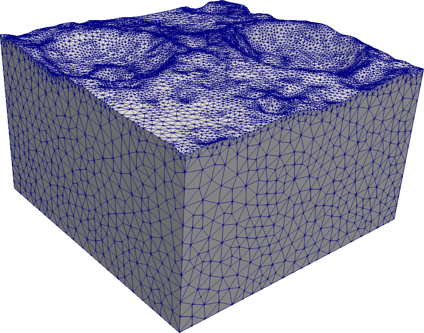
a Three-dimensional domain meshed with about $100\,000$ tetrahedron cells.

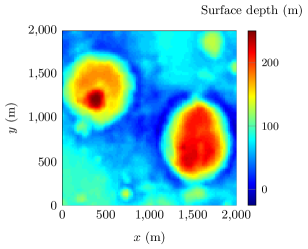
b Cartography of the topography.

Figure 3: Domain of interest of size $2\times 2\times 1$ ${\mathrm{km}}^{3}$, where the surface must be finely meshed to accurately capture the topography. Per convention, the positive values indicate the depth.

For the numerical computations, the use of the HDG discretization is appropriate and allow for a flexible framework using $\mathfrak{p}$-adaptivity. Indeed, the surface is finely mesh, such that low-order polynomials can be used in the area. On the other hand, in the deepest part where the cells are larger, we use higher order polynomials and benefit from the HDG discretization which disregards the inner dof for the global linear system. Following Remark 4, the order for the numerical trace $\lambda_{h}$ on a given face is taken to be the maximum order of the two adjacent cells that share this face.

In this experiment, the wave speed model contains layers of high-contrast velocities, and vary from $2000$ to $5500$ $\mathrm{m}\text{\,}{\mathrm{s}}^{-1}$, it is show in Figure 4 where we extract vertical and horizontal sections for visualization. Per simplicity, we consider a constant density with $\rho=$1000$$ $\mathrm{kg}\text{\,}{\mathrm{m}}^{-3}$. Following a seismic context, a Dirichlet boundary condition is imposed at the surface (with the topography), while absorbing boundary conditions are implemented on the other boundaries.

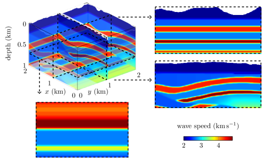
Figure 4: Target wave speed model for the inverse problem, for visualization, we extract vertical sections in $x=1$ $\mathrm{km}$ (top right) and $y=1$ $\mathrm{km}$ (bottom right), and a horizontal section in $z=$500$$ $\mathrm{m}$ (bottom left).

5.1 Synthetic partial reflection-data

We work with reflection data acquired from the surface only, with receivers positioned just underneath it to measure the pressure field. They are positioned to follow the topography in a lattice with about 75 $\mathrm{m}$ between each receivers, along the $x$ and $y$ directions. In total, we have 625 receivers. For the data, we consider a set of 100 point-sources (i.e., delta-Dirac function for the right-hand side of Eq. 3) that are independently excited. For each of the sources, the 625 receivers measure the resulting pressure field. The sources are also positioned to follow the topography, at the surface, in a lattice with about 190 $\mathrm{m}$ between them, for a total of 100 sources. This motivates the use of direct solvers which, as mentioned, allow for the fast resolution of all sources once the matrix is factorized. As all of the acquisition devices are restricted to the surface area, the partial data available only consist in reflection data, generated from only one-sided illumination.

We work with synthetic data but include white noise to make our experiments more realistic. The noise is incorporated in the data with a signal-to-noise ratio of $10$ $\mathrm{dB}$ for each measurements. In addition, the mesh and the order of the polynomial for the discretization differ between the generation of the data and the inversion procedure. Following the geophysical setup of this experiment, the available frequencies for the reconstruction are limited between $5$ and $15$ $\mathrm{Hz}$. In particular, the absence of low-frequency content in the data is an unavoidable difficulty of seismic applications [16, 67, 34].

5.2 Iterative reconstruction

We perform the iterative reconstruction using data with frequencies from $5$ $\mathrm{Hz}$ to $15$ $\mathrm{Hz}$, following a sequential progression, as advocated in [34]. The initial model is pictured in Figure 5: it consists in a one-dimensional variation (in depth only) where none of the sub-surface layers are initially known and with an inaccurate background velocity. In the inverse procedure, the model is represented as a piecewise-constant for simplicity, that is, we have one value of the parameter per cell.

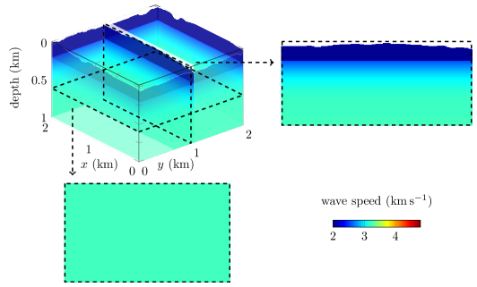
Figure 5: Initial wave speed model for the inverse problem, for visualization, we extract a vertical section in $y=1$ $\mathrm{km}$ (right), and a horizontal section in $z=$500$$ $\mathrm{m}$ (bottom left).

The search direction for the update of the wave speed model is computed using the non-linear conjugate gradient method, and only depends on the gradient of the misfit functional, cf. [57]. We perform $30$ iterations per frequency, for a total of $300$ iterations. The order of the polynomials for the basis functions changes with frequency (increases), while we use two meshes for the iterations: a coarse mesh for the first frequencies, from $5$ to $10$ $\mathrm{Hz}$, and a more refined one for higher frequencies, to capture more details. None of the two meshes for inversion are similar to the one used to generate the data, but we guarantee that the surface cells maintain the same topography. In Figure 6, we picture the reconstructed wave speed.

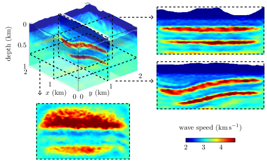
Figure 6: Reconstruction after iterative minimization with frequency up to $15$ $\mathrm{Hz}$, for visualization, we extract vertical sections in $x=1$ $\mathrm{km}$ (top right) and $y=1$ $\mathrm{km}$ (bottom right), and a horizontal section in $z=$500$$ $\mathrm{m}$ (bottom left).

We observe that the layers with high velocities are appropriately recovered: their positions and the values are accurate, except near the boundaries, due to the limited illumination. On the other hand, the lower values are not retrieved, and remain almost similar to the starting model. This is most likely due to the lack of background information in the starting model, which can only be recovered using low-frequency content in the data, cf. [39, 52, 34].

6 Perspectives

We have illustrated the use of HDG discretization in the context of time-harmonic inverse wave problems. The perspective is to handle larger-scale applications, using the smaller linear systems provided by the method, which only accounts for the degrees of freedom (dof) on the faces of the cells. Precisely, we have in mind problems made of multiple right-hand sides (e.g., with seismic acquisition) where the bottleneck is usually the memory needed for the matrix factorization. For an efficient implementation of the HDG discretization, we have the following requirements.

1. One needs to use polynomials of relatively high orders, because the inner-cell dof are omitted in the global linear system, i.e., the mesh must be composed of large cells.

2. On the other hand, large cells cannot be allowed on the whole domain (in order to appropriately represent the geometry) and we rely on $\mathfrak{p}$-adaptivity to adapt the polynomial orders to the size of the cells.

3. Because we use large cells, the model parameters must be carefully represented.

We provide here a preliminary experiment to illustrate, where we multiply by ten the size of the previous model, hence with a $20$$\times$$20$$\times$$10$ ${\mathrm{km}}^{3}$ domain. We generate a mesh of about $220\,000$ cells where, similarly as above, the surface is refined to correctly represent the topography.

Step 1: $\mathfrak{p}$-adaptivity

The first step is to select the order of the polynomials on each cell (as the dof of each cell are separated, see 2). We rely on the wavelength (that is, the ratio between the frequency and the wave speed on the cell) to select the order, and we illustrate in Figure 7 the resulting orders at $10$ $\mathrm{Hz}$ frequency. Here, the order of the polynomials varies from $3$ to $7$, such that the cells near surface, which are smaller to handle the topography, consequently use a low-order polynomial while the sub-surface layer, made of larger cells with low-velocity, need a high order. We also observe the sub-surface layer of increasing velocity, where the order is allowed to be reduced.

Step 2: model representation

Because of the large cells, the use of a piecewise-constant model parameters with one value per cell can lead to a coarse representation, that we illustrate in Figure 7. Therefore, we rely on a piecewise-polynomial model representation and illustrate in Figure 7 with polynomials of order 2 per cells to represent the wave speed. Clearly, the latter allows for a precise representation, removing the inaccuracies between cells. In this experiment where the above layer is mostly constant, we can even envision to use one polynomial on a group of cells instead of one per cell. Such models can be easily accounted for using the quadrature rules to evaluate the integrals, see Remark 3.

Figure 7: Extension of the model of Figure 3 to a domain of size $20$$\times$$20$$\times$$10$ ${\mathrm{km}}^{3}$. 7 Illustration of the $\mathfrak{p}$-adaptivity where the order of the polynomial varies per cell depending on the wavelength at $10$ $\mathrm{Hz}$. The order of the polynomial for the numerical trace on a face is selected as the maximal order of the two adjacent cells, see Remark 4. 7 Wave speed model using a piecewise-constant representation (one value per cell). 7 Wave speed model using piecewise-polynomial representation with functions of order 2 per cell.

Numerical cost

In Figure 8, we illustrate the solution of the forward problem with the pressure field for a single source at $6$ $\mathrm{Hz}$, where we follow the setup prescribed in Figure 7. The computation is performed using $360$ cores (using $10$ nodes with $4$ processors per node and $9$ threads per processor). The discretization problem has the following dimensions,

• The size of the linear system is $\widehat{N}_{\text{dof}}^{\Sigma}=$10\,993\,236$$.

• The number of volume dof per unknown is $\sum_{e}N_{\text{dof}}^{(e)}=$14\,812\,171$$, and we have four unknowns, i.e., the pressure and the vectorial velocity.

We see that the size of the linear system reduces by $25$ % the number of volume dof for one unknown, and by $80$ % if we consider the total size with the four unknowns. In this experiment, the matrix factorization requires $440$ $\mathrm{G}\mathrm{i}\mathrm{B}$ using the direct solver Mumps. The time to factorize the global matrix is of about $6$ $\min$, while the time to solve the local problems to assemble the volume solution is less than $1$ $\mathrm{s}$. It highlights that the second step of the method where one has to solve the local problems is very cheap compared to the resolution of the global linear system, in particular as it does not need any communication between the cells.

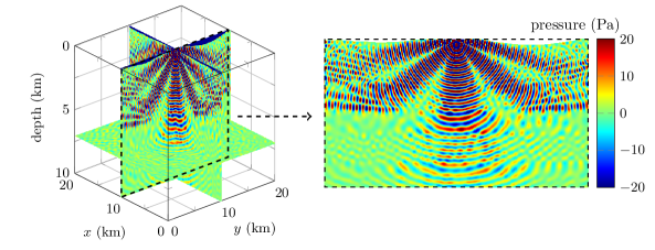
Figure 8: Real part of the time-harmonic pressure field at $6$ $\mathrm{Hz}$ on a domain of size $20$$\times$$20$$\times$$10$ ${\mathrm{km}}^{3}$, following the numerical setup given in Figure 7. For visualization, we extract a vertical section in $x=10$ $\mathrm{km}$ (right).

Remark 5.

Comparing with other discretization methods, where the linear system is made of the volume dof (see Figure 2), we can draw the following remarks,

• Standard DG results in a linear system of size the number of volume dof (see Figure 2b). To solve the first-order system with both the pressure field and velocity, it represents an increase of $539$ % compared to HDG. When solving the second-order system to only recover for the pressure field, it is an increase of $135$ %.

• Using Continuous Galerkin, let us first remind that it is much harder to employ $\mathfrak{p}$-adaptivity because the dof on the faces are shared (see Figure 2a). Then, assuming a constant order 7, the resulting linear system is increased by $490$ % and $122$ % compared to HDG, respectively for the first- and second-order systems.

$\triangle$

7 Conclusion

We have derived the adjoint-state method for the computation of the gradient of a functional in the framework of the Hybridizable Discontinuous Galerkin discretization in order to handle large-scale time-harmonic inverse problems using direct solvers to account for multiple right-hand sides. HDG reduces the size of the global linear system compared to other discretization methods, and it works with the first-order formulation of the forward problem. We have illustrated with the acoustic wave equation, where it gives the computational approximation for the pressure and the velocity fields at the same accuracy. The HDG method relies on two levels, a global system and local ones, which must be carefully addressed to obtain the adjoint-state where the matrix factorization of the forward problem can still be used for the backward problem. HDG allows to easily account for $\mathfrak{p}$-adaptivity, which is useful when some part of the mesh must be particularly refined to take into consideration the specificity of the problem, such that the geometry of the parameters or, as we have illustrated in our experiment, with the topography. We have given a preliminary insight to work with problems of larger scales, and we need to continue to investigate if HDG can help to fill the gap between the largest time and frequency-domain problems. Extension to elasticity is straightforward, and requires only minor modifications of the steps we have given, large-scale elastic inversion is part of our ongoing research.

References

- [1] M. Ainsworth, P. Monk, and W. Muniz, Dispersive and dissipative properties of discontinuous galerkin finite element methods for the second-order wave equation, Journal of Scientific Computing, 27 (2006), pp. 5–40, https://doi.org/10.1007/s10915-005-9044-x.
- [2] G. Alessandrini, M. V. De Hoop, F. Faucher, R. Gaburro, and E. Sincich, Inverse problem for the Helmholtz equation with Cauchy data: reconstruction with conditional well-posedness driven iterative regularization, ESAIM: M2AN, 53 (2019), pp. 1005–1030, https://doi.org/10.1051/m2an/2019009.
- [3] P. R. Amestoy, A. Buttari, J.-Y. L’Excellent, and T. A. Mary, Bridging the gap between flat and hierarchical low-rank matrix formats: The multilevel block low-rank format, SIAM Journal on Scientific Computing, 41 (2019), pp. A1414–A1442, https://doi.org/10.1137/18M1182760.
- [4] P. R. Amestoy, I. S. Duff, J.-Y. L’Excellent, and J. Koster, A fully asynchronous multifrontal solver using distributed dynamic scheduling, SIAM Journal on Matrix Analysis and Applications, 23 (2001), pp. 15–41, https://doi.org/10.1137/S0895479899358194.
- [5] P. R. Amestoy, A. Guermouche, J.-Y. L’Excellent, and S. Pralet, Hybrid scheduling for the parallel solution of linear systems, Parallel computing, 32 (2006), pp. 136–156, https://doi.org/10.1016/j.parco.2005.07.004.
- [6] H. Ammari, J. K. Seo, and L. Zhou, Viscoelastic modulus reconstruction using time harmonic vibrations, Mathematical Modelling and Analysis, 20 (2015), pp. 836–851, https://doi.org/10.3846/13926292.2015.1117531.
- [7] D. N. Arnold, F. Brezzi, B. Cockburn, and L. D. Marini, Unified analysis of discontinuous Galerkin methods for elliptic problems, SIAM journal on numerical analysis, 39 (2002), pp. 1749–1779, https://doi.org/10.1137/S0036142901384162.
- [8] H. Barucq, G. Chavent, and F. Faucher, A priori estimates of attraction basins for nonlinear least squares, with application to helmholtz seismic inverse problem, Inverse Problems, 35 (2019), p. 115004 (30pp), https://doi.org/https://doi.org/10.1088/1361-6420/ab3507.
- [9] H. Barucq, J. Diaz, R.-C. Meyer, and H. Pham, Implementation of hdg method for 2D anisotropic poroelastic first-order harmonic equations, research report, Inria Bordeaux Sud-Ouest ; Magique 3D ; Université de Pau et des Pays de l’Adour, 2020.
- [10] H. Barucq, F. Faucher, D. Fournier, L. Gizon, and H. Pham, Efficient computation of the modal outgoing green’s kernel for the scalar wave equation in helioseismology, Research Report RR-9338, Inria Bordeaux Sud-Ouest; Magique 3D; Max-Planck Institute for Solar System Research, April 2020.
- [11] H. Barucq, F. Faucher, and H. Pham, Localization of small obstacles from back-scattered data at limited incident angles with full-waveform inversion, Journal of Computational Physics, 370 (2018), pp. 1–24, https://doi.org/10.1016/j.jcp.2018.05.011.
- [12] H. Barucq, F. Faucher, and H. Pham, Outgoing solutions and radiation boundary conditions for the ideal atmospheric scalar wave equation in helioseismology, ESAIM: Mathematical Modelling and Numerical Analysis, 54 (2020), pp. 1111–1138, https://doi.org/10.1051/m2an/2019088.
- [13] J. Blackledge and L. Zapalowski, Quantitative solutions to the inverse scattering problem with applications to medical imaging, Inverse problems, 1 (1985), p. 17, https://doi.org/10.1088/0266-5611/1/1/004.
- [14] M. Bonnasse-Gahot, H. Calandra, J. Diaz, and S. Lanteri, Hybridizable discontinuous Galerkin method for the 2D frequency-domain elastic wave equations, Geophysical Journal International, 213 (2017), pp. 637–659, https://doi.org/10.1093/gji/ggx533.
- [15] R. Brossier, V. Etienne, S. Operto, and J. Virieux, Frequency-domain numerical modelling of visco-acoustic waves with finite-difference and finite-element discontinuous galerkin methods, Acoustic waves, (2010), pp. 434–p, https://doi.org/10.5772/9714.
- [16] C. Bunks, F. M. Saleck, S. Zaleski, and G. Chavent, Multiscale seismic waveform inversion, Geophysics, 60 (1995), pp. 1457–1473, https://doi.org/10.1190/1.1443880.
- [17] G. Chavent, Identification of functional parameters in partial differential equations, in Identification of Parameters in Distributed Systems, R. E. Goodson and M. Polis, eds., ASME, New York, 1974, pp. 31–48.
- [18] G. Chavent, Nonlinear least squares for inverse problems: theoretical foundations and step-by-step guide for applications, Springer Science & Business Media, 2010, https://doi.org/10.1007/978-90-481-2785-6.
- [19] M. Chin-Joe-Kong, W. A. Mulder, and M. Van Veldhuizen, Higher-order triangular and tetrahedral finite elements with mass lumping for solving the wave equation, Journal of Engineering Mathematics, 35 (1999), pp. 405–426, https://doi.org/10.1023/A:1004420829610.
- [20] Y. Choi, D.-J. Min, and C. Shin, Frequency-domain elastic full waveform inversion using the new pseudo-Hessian matrix: Experience of elastic Marmousi-2 synthetic data, Bulletin of the Seismological Society of America, 98 (2008), pp. 2402–2415, https://doi.org/10.1785/0120070179.
- [21] B. Cockburn, B. Dong, and J. Guzmán, A superconvergent ldg-hybridizable galerkin method for second-order elliptic problems, Mathematics of Computation, 77 (2008), pp. 1887–1916, https://doi.org/10.1090/S0025-5718-08-02123-6.
- [22] B. Cockburn, J. Gopalakrishnan, and R. Lazarov, Unified hybridization of discontinuous galerkin, mixed, and continuous galerkin methods for second order elliptic problems, SIAM Journal on Numerical Analysis, 47 (2009), pp. 1319–1365, https://doi.org/10.1137/070706616.
- [23] B. Cockburn, J. Gopalakrishnan, and F.-J. Sayas, A projection-based error analysis of hdg methods, Mathematics of Computation, 79 (2010), pp. 1351–1367, https://doi.org/10.1090/S0025-5718-10-02334-3.
- [24] B. Cockburn and C.-W. Shu, The local discontinuous galerkin method for time-dependent convection-diffusion systems, SIAM Journal on Numerical Analysis, 35 (1998), pp. 2440–2463, https://doi.org/10.1137/S0036142997316712.
- [25] D. Colton and R. Kress, Inverse acoustic and electromagnetic scattering theory, Applied mathematical sciences, Springer, New York, second ed., 1998, https://doi.org/10.1007/978-1-4614-4942-3.
- [26] B. T. Cox, J. G. Laufer, P. C. Beard, and S. R. Arridge, Quantitative spectroscopic photoacoustic imaging: a review, Journal of biomedical optics, 17 (2012), p. 061202, https://doi.org/10.1117/1.JBO.17.6.061202.
- [27] M. Dumbser and M. Käser, An arbitrary high-order discontinuous Galerkin method for elastic waves on unstructured meshes – II. The three-dimensional isotropic case, Geophysical Journal International, 167 (2006), pp. 319–336, https://doi.org/10.1111/j.1365-246X.2006.03120.x.
- [28] H. W. Engl, M. Hanke, and A. Neubauer, Regularization of inverse problems, vol. 375, Springer Science & Business Media, 1996, https://www.springer.com/gp/book/9780792341574.
- [29] B. Engquist and A. Majda, Absorbing boundary conditions for numerical simulation of waves, Proceedings of the National Academy of Sciences, 74 (1977), pp. 1765–1766, https://doi.org/10.1073/pnas.74.5.1765.
- [30] A. Ern and J.-L. Guermond, Theory and practice of finite elements, vol. 159, Springer Science & Business Media, 2013, https://doi.org/10.1007/978-1-4757-4355-5.
- [31] M. S. Fabien, M. G. Knepley, and B. M. Rivière, A hybridizable discontinuous galerkin method for two-phase flow in heterogeneous porous media, International Journal for Numerical Methods in Engineering, 116 (2018), pp. 161–177, https://doi.org/10.1002/nme.5919.
- [32] F. Faucher, Contributions to seismic full waveform inversion for time harmonic wave equations: stability estimates, convergence analysis, numerical experiments involving large scale optimization algorithms, PhD thesis, Université de Pau et Pays de l’Ardour, 2017.
- [33] F. Faucher, G. Alessandrini, H. Barucq, M. de Hoop, R. Gaburro, and E. Sincich, Full reciprocity-gap waveform inversion, enabling sparse-source acquisition, Geophysics, 85 (2020), pp. 1–82, https://doi.org/10.1190/geo2019-0527.1.
- [34] F. Faucher, G. Chavent, H. Barucq, and H. Calandra, A priori estimates of attraction basins for velocity model reconstruction by time-harmonic full waveform inversion and data-space reflectivity formulation, Geophysics, to appear (2020), https://doi.org/10.1190/geo2019-0251.1.
- [35] F. Faucher, M. V. De Hoop, and O. Scherzer, Reciprocity-gap misfit functional for distributed acoustic sensing, combining teleseismic and exploration data, ArXiv e-prints, (2020), pp. 1–16, https://arxiv.org/abs/2004.04580.
- [36] F. Faucher, O. Scherzer, and H. Barucq, Eigenvector models for solving the seismic inverse problem for the helmholtz equation, Geophysical Journal International, (2020), https://doi.org/10.1093/gji/ggaa009. ggaa009.
- [37] A. Fichtner, Full seismic waveform modelling and inversion, Springer Science & Business Media, 2011, https://doi.org/10.1007/978-3-642-15807-0.
- [38] A. Fichtner, B. L. Kennett, H. Igel, and H.-P. Bunge, Theoretical background for continental-and global-scale full-waveform inversion in the time–frequency domain, Geophysical Journal International, 175 (2008), pp. 665–685, https://doi.org/10.1111/j.1365-246X.2008.03923.x.
- [39] O. Gauthier, J. Virieux, and A. Tarantola, Two-dimensional nonlinear inversion of seismic waveforms; numerical results, Geophysics, 51 (1986), pp. 1387–1403, https://doi.org/10.1190/1.1442188.
- [40] R. Glowinski, Numerical Methods for Nonlinear Variational Problems, Springer-Verlag Berlin Heidelberg, 1985, https://doi.org/10.1007/978-3-662-12613-4.
- [41] R. Griesmaier and P. Monk, Error analysis for a hybridizable discontinuous galerkin method for the helmholtz equation, Journal of Scientific Computing, 49 (2011), pp. 291–310, https://doi.org/10.1007/s10915-011-9460-z.
- [42] M. Hanke, Conjugate gradient type methods for ill-posed problems, Routledge, 1995, https://doi.org/10.1201/9781315140193.
- [43] J. S. Hesthaven and T. Warburton, Nodal discontinuous Galerkin methods: algorithms, analysis, and applications, Springer Science & Business Media, 2007, https://doi.org/10.1007/978-0-387-72067-8.
- [44] B. Hustedt, S. Operto, and J. Virieux, Mixed-grid and staggered grid finite difference methods for frequency-domain acoustic wave modelling, Geophysical Journal International, 157 (2004), pp. 1269–1296, https://doi.org/10.1111/j.1365-246X.2004.02289.x. Geophysical Journal International, v. 157, n. 3, p. 1269-1296, 2004.
- [45] B. Kaltenbacher, Minimization based formulations of inverse problems and their regularization, SIAM Journal on Optimization, 28 (2018), pp. 620–645, https://doi.org/10.1137/17M1124036.
- [46] B. Kaltenbacher, A. Neubauer, and O. Scherzer, Iterative regularization methods for nonlinear ill-posed problems, vol. 6, Walter de Gruyter, 2008, https://doi.org/10.1515/9783110208276.
- [47] R. M. Kirby, S. J. Sherwin, and B. Cockburn, To CG or to HDG: a comparative study, Journal of Scientific Computing, 51 (2012), pp. 183–212, https://doi.org/10.1007/s10915-011-9501-7.
- [48] D. Komatitsch and J. Tromp, Introduction to the spectral element method for three-dimensional seismic wave propagation, Geophysical journal international, 139 (1999), pp. 806–822, https://doi.org/10.1046/j.1365-246x.1999.00967.x.
- [49] D. Komatitsch and J.-P. Vilotte, The spectral element method: an efficient tool to simulate the seismic response of 2D and 3D geological structures, Bulletin of the seismological society of America, 88 (1998), pp. 368–392.
- [50] P. Lailly, The seismic inverse problem as a sequence of before stack migrations, in Conference on Inverse Scattering: Theory and Application, J. B. Bednar, ed., Society for Industrial and Applied Mathematics, 1983, pp. 206–220.
- [51] J. L. Lions, Optimal control of systems governed by partial differential equations, vol. 1200, Springer Berlin, 1971.
- [52] Y. Luo and G. T. Schuster, Wave-equation traveltime inversion, Geophysics, 56 (1991), pp. 645–653, https://doi.org/10.1190/1.1443081.
- [53] L. Métivier, R. Brossier, Q. Mérigot, E. Oudet, and J. Virieux, Measuring the misfit between seismograms using an optimal transport distance: application to full waveform inversion, Geophysical Supplements to the Monthly Notices of the Royal Astronomical Society, 205 (2016), pp. 345–377, https://doi.org/10.1093/gji/ggw014.
- [54] L. Métivier, R. Brossier, J. Virieux, and S. Operto, Full waveform inversion and the truncated newton method, SIAM Journal on Scientific Computing, 35 (2013), pp. B401–B437, https://doi.org/10.1137/120877854.
- [55] N. C. Nguyen, J. Peraire, and B. Cockburn, An implicit high-order hybridizable discontinuous galerkin method for linear convection–diffusion equations, Journal of Computational Physics, 228 (2009), pp. 3232–3254, https://doi.org/10.1016/j.jcp.2009.01.030.
- [56] J. Nocedal, Updating quasi-Newton matrices with limited storage, Mathematics of computation, 35 (1980), pp. 773–782, https://doi.org/10.2307/2006193.
- [57] J. Nocedal and S. J. Wright, Numerical Optimization, Springer Series in Operations Research, 2 ed., 2006, https://doi.org/10.1007/b98874.
- [58] R.-E. Plessix, A review of the adjoint-state method for computing the gradient of a functional with geophysical applications, Geophysical Journal International, 167 (2006), pp. 495–503, https://doi.org/10.1111/j.1365-246X.2006.02978.x.
- [59] R. G. Pratt, C. Shin, and G. J. Hick, Gauss–newton and full newton methods in frequency–space seismic waveform inversion, Geophysical Journal International, 133 (1998), pp. 341–362, https://doi.org/10.1046/j.1365-246X.1998.00498.x.
- [60] A. Pulkkinen, B. T. Cox, S. R. Arridge, J. P. Kaipio, and T. Tarvainen, Quantitative photoacoustic tomography using illuminations from a single direction, Journal of biomedical optics, 20 (2015), p. 036015, https://doi.org/10.1117/1.JBO.20.3.036015.
- [61] J. O. Robertsson, A numerical free-surface condition for elastic/viscoelastic finite-difference modeling in the presence of topography, Geophysics, 61 (1996), pp. 1921–1934, https://doi.org/10.1190/1.1444107.
- [62] L. I. Rudin, S. Osher, and E. Fatemi, Nonlinear total variation based noise removal algorithms, Physica D: nonlinear phenomena, 60 (1992), pp. 259–268, https://doi.org/10.1016/0167-2789(92)90242-F.
- [63] O. Scherzer, Handbook of mathematical methods in imaging, Springer Science & Business Media, 2010, https://doi.org/10.1007/978-0-387-92920-0.
- [64] C. Shin and Y. H. Cha, Waveform inversion in the Laplace domain, Geophysical Journal International, 173 (2008), pp. 922–931, https://doi.org/10.1111/j.1365-246X.2008.03768.x.
- [65] C. Shin and Y. H. Cha, Waveform inversion in the Laplace Fourier domain, Geophysical Journal International, 177 (2009), pp. 1067–1079, https://doi.org/10.1111/j.1365-246X.2009.04102.x.
- [66] C. Shin, S. Pyun, and J. B. Bednar, Comparison of waveform inversion, part 1: conventional wavefield vs logarithmic wavefield, Geophysical Prospecting, 55 (2007), pp. 449–464, https://doi.org/10.1111/j.1365-2478.2007.00617.x.
- [67] L. Sirgue and R. G. Pratt, Efficient waveform inversion and imaging: A strategy for selecting temporal frequencies, Geophysics, 69 (2004), pp. 231–248, https://doi.org/10.1190/1.1649391.
- [68] A. Tarantola, Inversion of seismic reflection data in the acoustic approximation, Geophysics, 49 (1984), pp. 1259–1266, https://doi.org/10.1190/1.1441754.
- [69] B. Ursin and T. Toverud, Comparison of seismic dispersion and attenuation models, Studia Geophysica et Geodaetica, 46 (2002), pp. 293–320, https://doi.org/10.1023/A:1019810305074.
- [70] J. Virieux, Sh-wave propagation in heterogeneous media: velocity-stress finite-difference method, Geophysics, 49 (1984), pp. 1933–1942, https://doi.org/10.1190/1.1441605.
- [71] J. Virieux and S. Operto, An overview of full-waveform inversion in exploration geophysics, Geophysics, 74 (2009), pp. WCC1–WCC26, https://doi.org/10.1190/1.3238367.
- [72] S. Yakovlev, D. Moxey, R. M. Kirby, and S. J. Sherwin, To CG or to HDG: a comparative study in 3d, Journal of Scientific Computing, 67 (2016), pp. 192–220, https://doi.org/10.1007/s10915-015-0076-6.
- [73] Y. Yang, B. Engquist, J. Sun, and B. F. Hamfeldt, Application of optimal transport and the quadratic Wasserstein metric to full-waveform inversion, Geophysics, 83 (2018), pp. R43–R62, https://doi.org/10.1190/geo2016-0663.1.