Exploring non-singular black holes in gravitational perturbations

Abstract

We calculate gravitational perturbation quasinormal modes (QNMs) of non-singular Bardeen black holes (BHs) and singularity-free BHs in conformal gravity and examine their spectra in wave dynamics comparing with standard BHs in general relativity. After testing the validity of the approximate signal-to-noise ratio (SNR) calculation for different space based interferometers, we discuss the SNR of non-singular BHs in single-mode gravitational waveform detections in LISA, TianQin and TaiJi. We explore the impact of the Bardeen parameter and the conformal factor on the behavior of the SNR and find that in comparison with the standard Schwarzschild BHs, the increase of non-singular parameters leads to higher SNR for more massive non-singular BHs. We also examine the effect of the galactic confusion noise on the SNR and find that a dip appears in SNR due to such noise. For non-singular BHs, with the increase of the non-singular parameters the dip emerges for more massive BHs. It suggests a wider range of mass of non-singular black holes whose SNR will not be lowered by galactic noise, which implies the SNR for the super massive black holes centered at our galaxy will less likely to be influenced by galactic noise in non-singular black holes models than singular case in general relativity. We conduct Fisher analysis which suggests that the non-singular black holes parameters can be detected accurately with measurement errors as small as $\sim 10^{-4}-10^{-5}$. The detections of non-singular BHs are expected to be realized more likely by LISA or TaiJi.

I Introduction

Gravitational waves (GWs) were predicted by Einstein’s general relativity (GR) a century ago and since then huge amount of effort has been put into investigating the existence of GWs and thereby testing GR. Recently, the first GW event GW150914 with relatively high network SNR LIGOScientific:2018mvr was detected by LIGO Scientific Collaboration and Virgo Collaboration Abbott1 . More detections of GWs LIGOScientific:2018mvr ; Abbott:2020niy have been reported afterwards. The landmark detection of GWs ended the era of a single electromagnetic wave channel observation of our universe. Successful detections of GWs announced the dawn of multi-messenger astronomy with GW as a new probe to study our universe. As a new probe, people have proposed applications of GWs in the study of diversity subjects, such as searching dark matter Michimura:2020vxn ; DeRocco:2018jwe ; Obata:2018vvr ; Liu:2018icu ; Nagano:2019rbw ; Martynov:2019azm ; Grote:2019uvn ; Morisaki:2018htj ; Pierce:2018xmy ; Manley:2020mjq , exploring dark energy Weiner:2020sxn ; Garoffolo:2020vtd ; Singh:2020nna ; Noller:2020afd ; Yang:2020wby ; Li:2019ajo ; Zhang:2019ple , cosmological parameter estimation with GW standard siren Jin:2020hmc ; Zhao:2019gyk ; Zhang:2019mdf ; Zhang:2019loq ; Wang:2019tto ; Zhang:2019ylr , searching for modified theories of gravity Nunes:2020rmr ; Mastrogiovanni:2020gua ; Niu:2019ywx ; Ma:2019rei , etc.

The ground based interferometers (such as LIGO and Virgo) inevitably suffer from the gravity gradient noise and seismic noise which lead to the limitation that the detection of GWs with frequencies lower than 10Hz is extremely challenging. However, it is of great significance to probe GWs in lower frequency bands because a large number of GW sources containing rich physics are expected to fall in the frequency bands from millihertz to hertz Kormendy . Among these sources, the mergers of massive black hole (MBH) binaries with mass between $10^{3}M_{\odot}$ and $10^{7}M_{\odot}$ are expected to happen frequently Hu2017 ; Barausse:2014oca ; Klein:2015hvg with total number up to $\sim 332$ of mergers per year Klein:2015hvg , although there is no conclusive evidence yet. The existence of MBHs has been confirmed in the center of galaxies, for example a black hole named Sagittarius A* with mass about $4\times 10^{6}M_{\odot}$ was discovered in the center of our Milky Way Abuter:2018drb . To detect GWs from intermediate and super massive sources, we have to move our detectors to space. Laser Interferometer Space Antenna (LISA) amaroseoane2017laser , TaiJi Hu:2017mde and TianQin Luo are space based detectors to probe GWs with frequencies in the millihertz to hertz band.

Scientifically detecting GWs in space can disclose more physics of gravity. For the compact binaries, LIGO and Virgo detected GW emission from the merger of binary neutron stars (BNS) (e.g. GW170817 Abbott7 ). The characteristic of BNS was confirmed and the BNS was distinguished from the merger of binary black holes (BBHs) with the help of the electromagnetic observation (e.g. gamma-ray burst Monitor:2017mdv ; Goldstein:2017mmi and kilonova Arcavi:2017xiz ; Coulter:2017wya ; Lipunov:2017dwd ; Soares-Santos:2017lru ; Tanvir:2017pws ; Valenti:2017ngx ). Good sky location of the source can help for the detection of electromagnetic signals, just as in the case of event GW170817 Abbott7 . However the electromagnetic signal of BNS might not be detectable in some situations. One main reason is due to the large distance to the source and poor sky location which made the detection of electromagnetic signal quite difficult Abbott:2020uma ; Chen:2020fzm . Another reason might be that the initial BNS are massive enough and will directly collapse into black holes (BHs) Chen:2020fzm ; Shibata:2019wef ; Coughlin:2018fis ; Kiuchi:2019lls leaving negligible matter outside, then very faint electromagnetic signal would be created. It is expected that space based GW detectors can help uncover the tidal deformability in the binary system, whether it is zero or not Flanagan:2007ix can serve to determine the binary system being BBH or BNS. This signature can help understand better the galactic compact binaries. In addition, the quantum effect arising from the quantum correction to classical gravity theory around black hole event horizons can be encoded in GWs. It was argued that such quantum effect can be detected through the observation of GW echoes Cardoso:2016rao ; Cardoso:2016oxy . A tentative evidence for the echoes in GWs was disclosed in the LIGO observations Abedi:2016hgu , whereas it was claimed in Ref. Westerweck:2017hus ; Tsang:2019zra that current observations only provide low statistical significance for the existence of echoes. Nevertheless, it is expected that we can detect signals of echoes by the future space-based detectors or put strong constraints on alternative sources. The waveforms of GWs detected by ground-based detectors Abbott1 ; Abbott2 ; Abbott3 ; Abbott4 ; Abbott5 ; Abbott6 successfully confirmed GR in the nonlinear and strong-field regimes. However, we know that GR is not complete, and in particular it is plugged with the singularity problem, the non-renormalization problem and has difficulties in understanding the universe at very large scales. These provide the motivations for conceiving modified theories of gravity. Whether the meddling with GR can produce GWs to be detected by ground based or space based detectors is an interesting question to be studied.

In this work we will concentrate on the study of an alternative theory of GR to accommodate singularity free black hole solutions to avoid the singularity problem in GR. The existence of singularities in the solutions to Einstein’s field equations has been a longstanding problem. An idea considering the quantum effect of gravity was proposed to eliminate singularities. Following this idea some attempts have been made Ashtekar:2005qt ; Nicolini:2005vd ; LopezDominguez:2006wd ; Hossenfelder:2009fc ; Bojowald:2018xxu ; Ashtekar:2018lag ; Ashtekar:2018cay ; Bodendorfer:2019cyv ; Ashtekar:2020ifw ; Jusufi:2019caq ; BenAchour:2018khr ; BenAchour:2020bdt ; BenAchour:2020mgu to alleviate the singularity problem although a consistent quantum theory of gravity is still absent so far. To cure the shortcoming of GR at infrared and ultraviolet scales, a wide class of modified theories of gravity has been constructed with the purpose of addressing conceptual and experimental problems emerged in the fundamental physics and providing at least an effective description of quantum gravity Capozziello:2011et . Considering the non-physical characteristics of singularities, it is natural to find non-singular solutions to Einstein’s equations. The first non-singular black hole solution was found by Bardeen and it was later revealed that the nonlinear electromagnetic energy-momentum tensor playing the role of the source term in field equations AyonBeato:1998ub . In the conformal gravity frame, the black hole singularity could be removed under conformal transformations by taking advantage of the conformal symmetry of the spacetime Englert:1976ep ; tHooft:2011aa ; Dabrowski:2008kx ; Mannheim:2011ds ; Mannheim:2016lnx ; Modesto:2016max ; Bambi:2016wdn .

It is of great interest to study the wave dynamics of such non-singular BHs and distinguish them from black hole solutions in GR. The study of wave dynamics outside BHs has been an intriguing subject for the last few decades (for recent review, see for example Konoplya:2011qq ). A static observer outside a black hole can indicate successive stages of the wave evolution. After the initial pulse, the gravitational field outside the black hole experiences a quasinormal ringing, which describes the damped oscillations under perturbations in the surrounding geometry of a black hole with frequencies and damping times of the oscillations entirely fixed by the black hole parameters. The quasinormal mode (QNM) is believed as a unique fingerprint to directly identify the black hole existence and distinguish different black hole solutions. We will employ the 13-th order WKB method with averaging of the Pade approximations suggested first in Matyjasek:2017psv to compute the QNM of non-singular BHs and compare it with the result of wave dynamics in usual BHs in GR. Since the numerical method we apply here has very high accuracy Konoplya:2019hlu , we expect to find the special signatures of non-singular BHs in the wave dynamics.

The detection of QNMs can be realized through gravitational wave observations. From the observational point of view, we can calculate the signal-to-noise ratio (SNR) from the ringdown signals of GWs originated from the gravitational perturbations around BHs. Thus based on the precise QNM spectrum, we can obtain the SNR in GW observations. Different imprints in QNMs caused by different black hole configurations can be reflected in behaviors of the SNR. In order to distinguish different black hole solutions through the study of black hole spectroscopy, we require large SNR in the black hole ringdown phase. It was pointed out in Cardoso ; Berti:2009kk that to resolve either the frequencies or damping time of fundamental mode $(n=0)$ from the first overtone $(n^{\prime}=1)$ with the same angular dependence $(l=l^{\prime},m=m^{\prime})$, the critical value $\rho_{cri}$ of SNR is required to be around $\rho_{cri}\simeq 100$, while to resolve both the frequencies and damping time typically requires $\rho_{cri}\simeq 1000$. The large SNR can serve as a smoking gun in GW observations to identify the existence of non-singular black hole solutions in alternative theories of gravity. In the following discussion, we will not only examine the SNR in LISA, but also extend the calculation of SNR to other space based GW observations, such as TaiJi and TianQin, to check the feasibility of testing the existence of non-singular BHs.

The organization of the paper is as follows. In Section II, we introduce the calculation of SNR for single-mode waveform detections. In Section III, we calculate the QNMs and the SNR for non-singular BHs in conformal gravity. In Section IV, we generalize such calculations to the case for non-singular Bardeen BHs. In Section V, we calculate the errors in parameter estimation through a Fisher analysis. Finally in the last section we present our main conclusions. In Appendix A, we prove that the approximate formula in the SNR calculation developed in the context of LISA is general and can be applied to TaiJi and TianQin observations within acceptable errors.

II The SNR for single-mode waveform

In this section, we give a brief review on how to calculate the SNR for a single-mode wave detection. The basic idea was proposed in Cardoso for LISA and we generalize the method to discuss the SNR for Tianqin and TaiJi. We should point out that following analysis is only applicable to the ringdown stage of the gravitational waves.

The gravitational waveform composed of cross component $h_{\times}$ and plus component $h_{+}$ emitting from a perturbed black hole (or from the distorted final black hole merging from supermassive black hole pairs) can be expressed as

$$h_{+}+ih_{\times}=-\frac{2}{r^{4}}\int_{-\infty}^{+\infty}\frac{d\omega}{\omega^{2}}e^{i\omega t}\sum_{lm}S_{lm}(\iota,\beta)R_{lm\omega}(r),$$ (1)

where $R_{lm\omega}(r)$ is the radial Teukolsky function Teukolsky with the approximation $R_{lm\omega}(r)\sim r^{3}e^{-i\omega r}Z^{out}_{lm\omega}$ when $r\rightarrow\infty$. $Z_{lm\omega}^{out}$ is a complex amplitude. Now we assume that the gravitational waveform can be written as a formal QNM expansion and consider that the QNMs of the Schwarzschild and Kerr BHs always exist in pairs (because QNMs with positive number $m$ and negative $-m$ exist at the same time, we denote real and imaginary part of QNMs frequency with positive $m$ as $\{\omega_{lmn},\tau_{lmn}\}$, and for negative $-m$ as $\{\omega^{\prime}_{lmn},\tau^{\prime}_{lmn}\}$) which should be included in the waveform expansion. In this way we have

$$\begin{split}h_{+}+ih_{\times}&=\frac{1}{r}\sum_{lmn}\left\{e^{i\omega_{lmn}t}e^{-t/\tau_{lmn}}S_{lmn}(\iota,\beta)Z^{out}_{lmn}+e^{i\omega_{lmn}^{\prime}t}e^{-t/\tau_{lmn}^{\prime}}S_{lmn}^{\prime}(\iota,\beta)Z^{\prime out}_{lmn}\right\}\\ &=\frac{M}{r}\sum_{lmn}\left\{\mathcal{A}_{lmn}e^{i(\omega_{lmn}t+\phi_{lmn})}e^{-t/\tau_{lmn}}S_{lmn}(\iota,\beta)+\right.\\ &\left.\qquad\qquad\qquad\qquad\mathcal{A}^{\prime}_{lmn}e^{i(-\omega_{lmn}t+\phi_{lmn}^{\prime})}e^{-t/\tau_{lmn}}S_{lmn}^{\ast}(\iota,\beta)\right\},\end{split}$$ (2)

where we have rewritten the complex $Z^{out}_{lmn}$ in terms of a real amplitude $\mathcal{A}_{lmn}$ and a real phase $\phi_{lmn}$, and we factor out the black hole mass $M$ by $Z^{out}_{lmn}=M\mathcal{A}_{lmn}e^{i\phi_{lmn}}$. In the above expansion, $S_{lm}(\iota,\beta)$ stands for spin weighted spheroidal harmonics whose complex conjugate is denoted by $S_{lmn}^{\ast}(\iota,\beta)$, $\iota$ and $\beta$ are angular variables, and $l$, $m$ are indices analogous to those for standard spherical harmonics corresponding to a particular case of $S_{lmn}(\iota,\beta)$ in which both the perturbation field and black hole spin are zero, $n$ denotes the overtone number. Note that we have the complex QNM frequency $\omega=\omega_{lmn}+i/\tau_{lmn}$, where the real part denotes the oscillation frequency $\omega_{lmn}=2\pi f_{lmn}$ and the imaginary part $\tau_{lmn}$ is the damping time of the perturbation oscillation. For a single given mode labeled by ($l,m,n$), the real waveform measured at the detector can be expressed as a linear superposition of $h_{+}$ and $h_{\times}$

$$h_{+}=\frac{M}{r}\mathfrak{R}\left[\mathcal{A}_{lmn}^{+}e^{i(\omega_{lmn}t+\phi_{lmn}^{+})}e^{-t/\tau_{lmn}}S_{lmn}(\iota,\beta)\right],$$ (3a)

$$h_{\times}=\frac{M}{r}\mathfrak{I}\left[\mathcal{A}_{lmn}^{\times}e^{i(\omega_{lmn}t+\phi_{lmn}^{\times})}e^{-t/\tau_{lmn}}S_{lmn}(\iota,\beta)\right],$$ (3b)

in which we have the relation $\mathcal{A}_{lmn}^{+,\times}e^{i\phi_{lmn}^{+,\times}}=\mathcal{A}_{lmn}e^{i\phi_{lmn}}\pm\mathcal{A}_{lmn}^{\prime}e^{-i\phi_{lmn}^{\prime}}$, where the signs $+(-)$ correspond to the $+(\times)$ polarizations respectively. The waveform $h$ detected by a detector is given by

$$h =h_{+}F_{+}(\theta_{S},\phi_{S},\psi_{S},f)+h_{\times}F_{\times}(\theta_{S},\phi_{S},\psi_{S},f),$$ (4)

where $F_{+,\times}$ are frequency dependent pattern functions (response functions) depending on the orientation $\psi_{S}$ of the detector and the direction ($\theta_{S},\phi_{S}$) of the source. For LIGO (in the long wavelength limit), we have

$$F_{+} =\frac{1}{2}(1+\cos^{2}\theta_{S})\cos 2\phi_{s}\cos 2\psi_{S}-\cos\theta_{S}\sin 2\phi_{S}\sin 2\psi_{S},$$ (5a)

$$F_{\times} =\frac{1}{2}(1+\cos^{2}\theta_{S})\sin 2\phi_{s}\cos 2\psi_{S}+\cos\theta_{S}\sin 2\phi_{S}\cos 2\psi_{S},$$ (5b)

which are independent of the frequency. The sky and polarization averaged SNR is Cardoso ; liuchang ,

$$\rho^{2}=4\int_{0}^{\infty}\frac{\langle\tilde{h}^{\ast}(f)\tilde{h}(f)\rangle}{S_{N}(f)}df=4\int_{0}^{\infty}\frac{|\tilde{h}_{+}|^{2}+|\tilde{h}_{\times}|^{2}}{S_{n}(f)}df,$$ (6a)

$$S_{n}(f)=\frac{S_{N}(f)}{\mathcal{R}(f)},$$ (6b)

$$\mathcal{R}(f)=\langle|F_{+}(f)|^{2}\rangle=\langle|F_{\times}(f)|^{2}\rangle,$$ (6c)

where $\tilde{h}(f)$ is the Fourier transform of the waveform, $S_{N}(f)$ is the noise spectral density of the detector, $S_{n}(f)$ is the detector sensitivity, $\mathcal{R}(f)$ is the sky/polarization averaged response function. The sky/polarization averaged is defined by

$$\langle X\rangle=\frac{1}{4\pi^{2}}\int_{0}^{\pi}d\psi\int_{0}^{2\pi}d\phi\int_{0}^{\pi}X\sin\theta d\theta$$ (7)

Especially, the response function $\mathcal{R}$ for LIGO is liuchang

$$\mathcal{R}=\langle|F_{+}|^{2}\rangle=\langle|F_{\times}|^{2}\rangle=\frac{1}{32}\int_{-1}^{1}(1+6x^{2}+x^{4})dx=\frac{1}{5},\quad x=-\cos\theta$$ (8)

while the full expressions of $F_{+}(f)$ and $F_{\times}(f)$ for LISA, TianQin and TaiJi are much more complicated and can be found in Larson:1999we ; Liang:2019pry . We perform the Fourier transform of the waveform by using the relation

$$\int_{-\infty}^{\infty}e^{i\omega t}\left(e^{\pm i\omega_{lmn}t-|t|/\tau_{lmn}}\right)dt=\frac{2/\tau_{lmn}}{(1/\tau_{lmn})^{2}+(\omega\pm\omega_{lmn})^{2}}\equiv 2b_{\pm}.$$ (9)

Based on Eq. (9) we can easily work out the Fourier transform of the plus and cross components,

$$\tilde{h}_{+} =\frac{1}{\sqrt{2}}\frac{M}{r}\mathcal{A}_{lmn}^{+}\left[e^{i\phi_{lmn}^{+}}S_{lmn}b_{+}+e^{-i\phi_{lmn}^{+}}S_{lmn}^{\ast}b_{-}\right],$$ (10a)

$$\tilde{h}_{\times} =-\frac{1}{\sqrt{2}}\frac{iM}{r}\mathcal{A}_{lmn}^{\times}\left[e^{i\phi_{lmn}^{\times}}S_{lmn}b_{+}-e^{-i\phi_{lmn}^{\times}}S_{lmn}^{\ast}b_{-}\right].$$ (10b)

We add a correction factor $1/\sqrt{2}$ to serve as a compensation in amplitude because we are using the FH convention (developed by Flanagan and Hughes Flanagan:1997sx ) to calculate the SNR. In the FH convention, the waveform for $t<0$ is assumed to be identical to waveform for $t>0$ and therefore we can replace the decay factor $e^{-t/\tau_{lmn}}$ with $e^{-|t|/\tau_{lmn}}$ in the Fourier transform such that a compensation is needed for the doubling. Then we can insert Eq. (10) into Eq. (6a) and do the integration to calculate SNR. However, as described in Cardoso , a simple analytical formula of SNR can be derived by making some approximations in the calculation. In this way, we have the SNR expression as Cardoso ,

$$\rho_{FH}=\frac{1.31681\times 10^{4}}{\mathcal{F}_{lmn}}\left(\frac{\epsilon_{rd}}{0.03}\right)^{\frac{1}{2}}\left(\frac{(1+z)M}{10^{6}M_{\odot}}\right)^{\frac{3}{2}}\left(\frac{1\,\mathrm{Gpc}}{D_{L}(z)}\right)\left(\frac{S_{0}}{S_{n}(f_{lmn})}\right)^{\frac{1}{2}}\frac{2Q_{lmn}}{\sqrt{1+4Q_{lmn}^{2}}},$$ (11)

where $S_{0}=1.59\times 10^{-41}\mathrm{Hz}^{-1}$, $\mathcal{F}_{lmn}$ is the dimensionless frequency defined by $\mathcal{F}_{lmn}=M\omega_{lmn}$, $\epsilon_{rd}$ is the radiation efficiency, $M_{\odot}$ is the solar mass and $M$ is the black hole (source) mass, $Q_{lmn}$ is a dimensionless quality factor of QNMs defined by

$$Q_{lmn}=\pi f_{lmn}\tau_{lmn}=\frac{1}{2}\omega_{lmn}\tau_{lmn},$$ (12)

and $D_{L}(z)$ is the luminosity distance which can be expressed as a function of cosmological redshift $z$ of the source in the standard flat $\Lambda$CDM cosmological model as

$$D_{L}(z)=\frac{1+z}{H_{0}}\int_{0}^{z}\frac{dz^{\prime}}{\sqrt{\Omega_{M}(1+z^{\prime})^{3}+\Omega_{\Lambda}}}.$$ (13)

We shall take the matter density $\Omega_{M}=0.32$, the dark energy density $\Omega_{\Lambda}=0.68$ and the Hubble constant $H_{0}=67\,\mathrm{km}\,\mathrm{s}^{-1}\mathrm{Mpc}^{-1}$. Eq. (11) was derived in the context of LISA by making some approximations such as $S_{lmn}\simeq\mathfrak{R}(S_{lmn})$ and large $Q_{lmn}$ limit. We will show that these approximations and the derivation steps of Eq. (11) are not dependent on specific interferometric detectors, therefore Eq. (11) could be applied to other space based detectors such as TianQin and TaiJi. We will discuss the generality of the approximate SNR formula Eq. (11) in more details in Appendix A, and show that this formula is applicable to TianQin and TaiJi.

For the calculation of SNR, we will adopt the following noise and response functions for all three space based detectors Cornish:2001qi

$$S_{N}(f) =\frac{4S_{a}}{(2\pi f)^{4}L^{2}}\left(1+\frac{10^{-4}\mathrm{Hz}}{f}\right)+\frac{S_{x}}{L^{2}},$$ (14a)

$$\mathcal{R}(f) =\frac{3}{10}\left[1+0.6\left(\frac{f}{f_{\ast}}\right)^{2}\right]^{-1},$$ (14b)

in which $L$ is the detector arm length and $f_{\ast}=c/(2\pi L)$ is the transfer frequency, $S_{a}$ is the acceleration noise and $S_{x}$ is the position noise of the instruments, and we list these parameters for three detectors in Table. 1.

	LISA	TianQin	TaiJi
$L$	$2.5\times 10^{9}\mathrm{m}$	$\sqrt{3}\times 10^{8}\mathrm{m}$	$3\times 10^{9}\mathrm{m}$
$\sqrt{S_{a}}$	$3\times 10^{-15}\mathrm{ms}^{-2}/\mathrm{Hz}^{1/2}$	$10^{-15}\mathrm{ms}^{-2}/\mathrm{Hz}^{1/2}$	$3\times 10^{-15}\mathrm{ms}^{-2}/\mathrm{Hz}^{1/2}$
$\sqrt{S_{x}}$	$1.5\times 10^{-11}\mathrm{m}/\mathrm{Hz}^{1/2}$	$10^{-12}\mathrm{m}/\mathrm{Hz}^{1/2}$	$8\times 10^{-12}\mathrm{m}/\mathrm{Hz}^{1/2}$

Table 1: Parameters of all three space based detectors.

In addition to the noise of the detectors, an effective noise can be generated by the galactic binaries. For LISA, the galactic noise can be well fitted as liuchang ; Cornish2017

$$S_{c}(f)=Af^{-7/3}e^{-f^{\alpha}+\beta f\sin(\kappa f)}[1+\tanh(\gamma(f_{k}-f))]\mathrm{Hz}^{-1},$$ (15)

and the total sensitivity can be obtained by adding $S_{c}(f)$ to $S_{n}(f)$. The effects of the galactic noise on the SNR for LISA will be discussed later, and the parameters we are going to use for the four year mission lifetime are $A=9\times 10^{-45}$, $\alpha=0.138$, $\beta=-221$, $\kappa=521$, $\gamma=1680$, and $f_{k}=0.0013$ liuchang .

We show the root sensitivity curve for LISA, TianQin and TaiJi in Fig. 1, from which we can see that the sensitivity value of TianQin is higher than that of LISA in the frequency range $f\lesssim 0.01\mathrm{Hz}$ and the sensitivity value of TianQin can be higher than Taiji when $f\lesssim 0.04\mathrm{Hz}$. For the rest regions of frequency respectively, the LISA and TaiJi have higher sensitivity than that of TianQin, which suggests that comparing to TianQin, LISA and TaiJi are better for gravitational wave detections at lower frequencies (usually corresponds to higher black hole mass), while for higher frequencies we should turn to count on TianQin. In addition, we can see that the sensitivity of TaiJi is always lower than that of LISA in the whole frequency band which implies that TaiJi can be more sensitive to detect the gravitational wave signals emitted from the same source when compared with LISA.

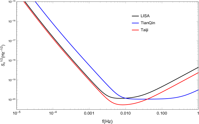
Figure 1: The root sensitivity curves for LISA, TianQin and TaiJi.

III SNR for non-singular BHs in conformal gravity

III.1 Quasinormal modes of non-singular BHs in conformal gravity

The metric of non-singular BHs in conformal gravity can be expressed as Bambi1

$$ds^{2}=S(r)ds_{\mathrm{Schw}}^{2}=-S(r)f(r)dt^{2}+\frac{S(r)}{f(r)}dr^{2}+S(r)r^{2}d\Omega^{2},$$ (16)

where $ds_{\mathrm{Schw}}^{2}$ is the Schwarzschild spacetime line element, with $f(r)=1-2M/r$, the factor $S(r)$ is Bambi1

$$S(r)=\left(1+\frac{L^{2}}{r^{2}}\right)^{2N},$$ (17)

and $N$ is an arbitrary positive integer and $L$ is a new length scale. The additional conformal factor $S(r)$ making the spacetime singularity-free distinguishes the metric (16) from the Schwarzschild metric, and the metric (16) can reduce to Schwarzschild form when $S(r)\rightarrow 1$, i.e. $N\rightarrow 0$ or $L\rightarrow 0$. We will show that the non-zero parameters $N,L$ will influence the dynamical behavior reflected by QNMs of BHs under gravitational perturbations. Since QNMs can disclose the black hole fingerprint, it can differentiate such non-singular BHs from the Schwarzschild black hole, as we will discuss in the following.

The master equation for the axial gravitational perturbation reads Chen:2019iuo

$$\frac{d^{2}H^{(-)}}{dr_{\ast}^{2}}+(\omega^{2}-V(r))H^{(-)}=0,$$ (18)

where we have used tortoise radius defined by $dr/dr_{\ast}=f(r)$, $H^{(-)}$ is the radial part of the axial gravitational perturbation, $\omega$ is the QNM frequency, the effective potential $V$ is Chen:2019iuo

$$V(r)=f(r)\left\{\frac{l(l+1)}{r^{2}}-\frac{2}{r^{2}}-Z\frac{d}{dr}\left(\frac{f(r)dZ/dr}{Z^{2}}\right)\right\},$$ (19)

and $Z(r)=\sqrt{S(r)}r$.

In Chen:2019iuo , the 6th order WKB method was adopted to compute the QNM of the non-singular black hole configuration. In our numerical computation, we employ the 13th order WKB approximation. In the study of gravitational perturbations in the Schwarzschild black hole Matyjasek:2017psv , comparing with the accurate numerical result, it was found that the 13th order WKB is more precise than the 6th WKB approach. It was argued that the WKB approximation works in satisfactory accuracy in calculating the QNM once $l>>n$ Iyer:1986np , while does not work well for high overtone modes. In Chen:2019iuo the discussion on the QNM was only limited to the lowest QNM for the gravitational perturbation. Including the Pade approximation, it was observed that there is a great increase of accuracy in calculating the QNM by using the WKB approach, furthermore with averaging of the Pade approximation accurate calculations can be achieved not only in the lowest mode, but also for the overtone modes with slightly bigger $n$ than $l$, however the numerical results are still not much reliable for $n\gg l$, even if the Pade approximation is included Matyjasek:2017psv .

In our numerical computation, we employ the 13th order WKB approximation method with averaging of the Pade approximations Matyjasek:2017psv to calculate the QNMs of the axial gravitational perturbation on the background of non-singular BHs. We show our results in Tables LABEL:table1 and LABEL:table2 where we express the QNM frequency in a dimensionless variable $M\omega$.

Table 2: Quasinormal frequency $M\omega$ for non-singular BHs in conformal gravity for parameter $L=2$.

$l$	$n$	$N=0$	$N=2$	$N=5$	$N=10$
$2$	$0\,$	$0.373675-0.088964i\,$	$0.409160-0.121392i\,$	$0.715683-0.134492i\,$	$1.372383-0.139325i$
	$1$	$0.346827-0.273930i$	$0.407758-0.370858i$	$0.719270-0.403565i$	$1.376117-0.417754i$
	$2$	$0.299998-0.478098i$	$0.414498-0.620991i$	$0.727050-0.672962i$	$1.383599-0.695444i$
$3$	$0$	$0.599443-0.092703i$	$0.620553-0.107015i$	$0.855703-0.125041i$	$1.450989-0.135461i$
	$1$	$0.582643-0.281297i$	$0.604412-0.331714i$	$0.853220-0.377014i$	$1.452762-0.406564i$
	$2$	$0.551686-0.479087i$	$0.589888-0.569715i$	$0.851142-0.632531i$	$1.456717-0.678002i$
	$3$	$0.511943-0.690318i$	$0.584544-0.815114i$	$0.851857-0.890962i$	$1.463341-0.949499i$
$4$	$0$	$0.809178-0.094163i$	$0.825032-0.102217i$	$1.013367-0.117947i$	$1.549660-0.131294i$
	$1$	$0.796631-0.284334i$	$0.810029-0.311229i$	$1.007860-0.356078i$	$1.549669-0.394338i$
	$2$	$0.772709-0.479908i$	$0.786423-0.534230i$	$0.999971-0.599176i$	$1.550292-0.658511i$
	$3$	$0.739836-0.683924i$	$0.766779-0.768643i$	$0.992948-0.846952i$	$1.552405-0.923937i$
	$4$	$0.701514-0.898237i$	$0.754662-1.007982i$	$0.988570-1.097952i$	$1.556748-1.190222i$
$5$	$0$	$1.012295-0.094870i$	$1.025096-0.100075i$	$1.181610-0.112849i$	$1.664843-0.127206i$
	$1$	$1.002221-0.285817i$	$1.013275-0.302492i$	$1.174978-0.340491i$	$1.663474-0.382215i$
	$2$	$0.982695-0.480328i$	$0.991012-0.512278i$	$1.164029-0.573071i$	$1.661378-0.638801i$
	$3$	$0.955004-0.680556i$	$0.963850-0.734449i$	$1.152084-0.811398i$	$1.659565-0.897424i$
	$4$	$0.921081-0.888197i$	$0.940140-0.967011i$	$1.141652-1.054348i$	$1.659055-1.157978i$
	$5$	$0.883335-1.104182i$	$0.840158-1.120908i$	$1.133807-1.300278i$	$1.660604-1.419940i$

Table 3: Quasinormal frequency $M\omega$ for non-singular BHs in conformal gravity for parameter $N=2$.

$l$	$n$	$L=0$	$L=2$	$L=5$	$L=15$
$2$	$0\,$	$0.373675-0.088964i\,$	$0.409161-0.121392i\,$	$0.500121-0.105834i\,$	$0.530178-0.094147i$
	$1$	$0.346827-0.273931i$	$0.407758-0.370858i$	$0.496880-0.317166i$	$0.514476-0.284905i$
	$2$	$0.299998-0.478098i$	$0.414498-0.620991i$	$0.489883-0.526622i$	$0.484316-0.483647i$
$3$	$0$	$0.599443-0.092703i$	$0.620553-0.107015i$	$0.686818-0.101541i$	$0.708826-0.094852i$
	$1$	$0.582643-0.281297i$	$0.604412-0.331714i$	$0.679594-0.305861i$	$0.696048-0.286379i$
	$2$	$0.551686-0.479087i$	$0.589888-0.569715i$	$0.667081-0.512816i$	$0.671468-0.483427i$
	$3$	$0.511943-0.690318i$	$0.584544-0.815114i$	$0.648889-0.720679i$	$0.637497-0.689529i$
$4$	$0$	$0.809178-0.094163i$	$0.825032-0.102217i$	$0.876184-0.099544i$	$0.893459-0.095293i$
	$1$	$0.796631-0.284334i$	$0.810029-0.311229i$	$0.868380-0.299798i$	$0.882860-0.287183i$
	$2$	$0.772709-0.479908i$	$0.786423-0.534230i$	$0.853993-0.502905i$	$0.862299-0.482970i$
	$3$	$0.739836-0.683924i$	$0.766779-0.768643i$	$0.834321-0.709301i$	$0.833181-0.685113i$
	$4$	$0.701514-0.898237i$	$0.754662-1.007982i$	$0.809681-0.918896i$	$0.797793-0.895593i$
$5$	$0$	$1.012295-0.094871i$	$1.025096-0.100075i$	$1.066719-0.098481i$	$1.080916-0.095562i$
	$1$	$1.002221-0.285817i$	$1.013275-0.302492i$	$1.059305-0.296361i$	$1.071930-0.287641i$
	$2$	$0.982695-0.480328i$	$0.991012-0.512278i$	$1.045228-0.496726i$	$1.054373-0.482565i$
	$3$	$0.955004-0.680556i$	$0.963851-0.734449i$	$1.025583-0.700485i$	$1.029119-0.682139i$
	$4$	$0.921081-0.888197i$	$0.940140-0.967011i$	$1.001235-0.907965i$	$0.997555-0.887945i$
	$5$	$0.883335-1.104182i$	$0.840158-1.120908i$	$0.972539-1.119446i$	$0.961550-1.101097i$

In Table. LABEL:table1 where we fix the parameter $L$, we find that with the increase of $N$ both the real part representing the oscillation frequency and the magnitude of the imaginary part relating to the damping time of QNMs will increase, which implies that with the increase of the parameter $N$ in the non-singular black hole in conformal gravity, the gravitational perturbation can have more oscillations but die out faster. Comparing to the non-singular black hole backgrounds, we find that the perturbation of the Schwarzschild black hole with $N=0$ can last longer. Our result confirms that reported in Chen:2019iuo where they limited their discussion to a fixed angular index $l$. Since we have adopted the Pade approximation, we can accurately calculate QNMs for the change of $n,l$ until $n=l$ (to keep numerical accuracy, $n>l$ is not considered in our discussion). In the Schwarzschild background, for the same overtone mode when the angular index $l$ becomes higher, we observe that the real parts of frequency are always higher, while the imaginary part is higher for $n\leq 2$, but decreases when $n>2$. However this property does not hold for non-singular BHs with $N\neq 0$. In non-singular holes, for the same overtone modes the higher angular number $l$ always results in a higher real part of the frequency but smaller imaginary part of the frequency, which suggests that for the same overtone mode the perturbation with higher angular index may last longer for non-singular BHs while in the Schwarzschild black hole perturbation the mode $l=2,n=0$ is always the longest one.

In Table. LABEL:table2 we present the frequencies of QNMs for a fixed $N$ parameter. With the increase of $L$, the real part of QNMs monotonously increases while the imaginary part increases from $L=0$ to $L=2$ but then decreases continuously with the further increase of $L$. This behavior agrees to the result reported in Chen:2019iuo for a fixed angular index $l$. Employing the Pade approximation, we accurately calculated QNMs with our 13th WKB approach for different $n,l$ even when $n=l$. Similar to the Schwarzschild black hole, for the non-singular BHs we find that for the same overtone modes, with the increase of the angular number $l$, the real part of the frequency increases. The absolute imaginary part of the frequency for non-singular BHs presents different behaviors from that of the Schwarzschild background when $L$ is not big enough. For the same overtone mode, with the increase of the angular number $l$, the absolute imaginary part of the frequency for a non-singular black hole decreases instead of increasing as in the Schwarzschild background. This is consistent with the picture we learn from Table.LABEL:table1, for the same overtone mode the perturbation for a non-singular black hole with a larger angular index $l$ may last longer, which is different from the case in the Schwarzschild background, where the fundamental mode $n=0,l=2$ always dominates. The result of changing $L$ looks more complicated than that for the change of $N$ given above. When $L=15$, the QNM frequencies return to the similar behavior with the change of $n,l$ to that in the Schwarzschild background. In this case, for the same overtone number, we can see that the real part of the frequency increases monotonously with the angular number $l$, while for $n\leq 1$ the imaginary part is higher for larger $l$, but for $n>1$ it decreases when increasing $l$.

Precise numerical results of the QNM frequencies for different $(n,l)$ are useful to calculate the multi-mode SNR of this non-singular black hole. However in this work we will concentrate on the single-mode SNR. Different from the Schwarzschild black hole, it looks that in the non-singular black hole background the mode $n=0,l=2$ is not apparently the dominant mode (here ‘dominant mode’ means the mode with slowest damping rate corresponding to smallest value of $-\mathrm{Im}\,\omega$). Instead, for the same overtone mode, the imaginary frequency for a bigger angular index implies that the perturbation may last longer in the non-singular black hole. However, we notice that in the limit $l\rightarrow\infty$, the effective potential $V(r)\approx f(r){l^{2}}/{r^{2}}$, which reduces to that of Schwarzschild BHs, which makes it difficult to distinguish the modes between the non-singular black hole and the Schwarzschild black hole in the large $l$ limit. In the face of complicated data, actually a criterion to determine the dominant mode was suggested in Wang:2004bv . We redefine the dominant mode by choosing min$\{\sqrt{\omega_{R}^{2}+\omega_{I}^{2}}\}$. Applying this criterion, we find that it is always the $n=0,l=2$ mode that serves the dominant mode in the perturbation, which holds also in the non-singular black hole. If we look at the relation Eq. (45) between the GW amplitude $\mathcal{A}_{lm}$ and the energy radiation efficiency $\epsilon_{rd}$, the $n=0,l=2$ mode always has the strongest amplitude corresponding to more powerful energy in this mode. This further guarantees that the $n=0,l=2$ mode dominates in the perturbation in the non-singular black hole. Now we can compare the same dominant single-mode SNR for the non-singular black hole and the Schwarzschild black hole, which allows us to explore their imprints in GWs.

III.2 SNR by LISA, TianQin and TaiJi

In this subsection we calculate the SNR for LISA, TianQin and TaiJi by using the QNMs we have obtained for non-singular BHs in conformal gravity. We explore the SNR related to the dominant mode $n=0,l=2$ in both of the non-singular and Schwarzschild BHs. At first we would like to focus on the discussion of SNR for LISA, and then we will take TianQin and TaiJi into consideration for comparisons. In the calculation of SNR, we would like to set an optimistic value of radiation efficiency $\epsilon_{rd}=3\%$ assumed in Flanagan:1997sx , which is based on quadrupole-formula-based estimate of the QNMs amplitude when the distortion of the horizon of the black hole is of order unity Flanagan:1997sx , as well as a pessimistic value $\epsilon_{rd}=0.1\%$ corresponding to the estimates for the energy emitted in the head-on collision of equal-mass black holes Sperhake:2005uf .

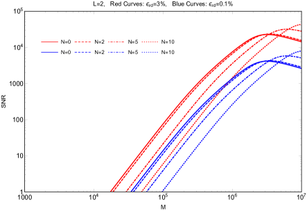
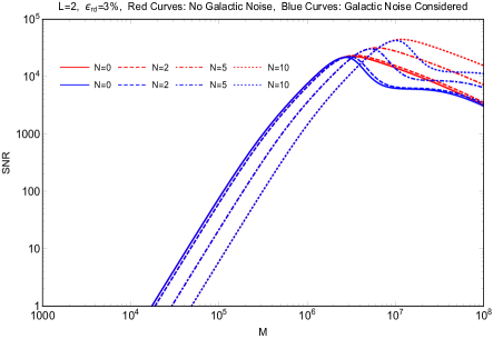
Figure 2: The SNR behavior of LISA with the change of the black hole mass $M$ at a distance $D_{L}=3\,\mathrm{Gpc},z=0.54$ with the angular number $l=2$ in QNMs. For each plot we have fixed the value of $L$ but changing $N$. For the left plot, the red curves and blue curves correspond to the radiation efficiency $\epsilon_{rd}=3\%$ and $0.1\%$, respectively, while for the right plot we set $\epsilon_{rd}=3\%$, and the red curves denote the SNR without including the galactic noise and the blue curves denote the SNR affected by the galactic noise.

In Fig. 2 we show the SNR curve by fixing the parameter $L$, while changing the parameter $N$. We can see that with the increase of the mass, the SNR will grow, which implies that LISA is more sensitive to GW signals generated by BHs with greater mass. For the Schwarzschild black hole with $N=0$, the SNR will reach the maximum when the black hole mass becomes $\sim 10^{6}M_{\odot}$. Thus for the Schwarzschild black hole LISA is most sensitive when the black hole mass is around $2\times 10^{6}M_{\odot}$. Considering the non-singular black hole with bigger $N$, we see that the SNR is smaller than that of the Schwarzschild black hole when the black hole mass is below $2\times 10^{6}M_{\odot}$ and with the increase of $N$, the SNR is more suppressed when the black hole mass is within this value. However when the black hole is more massive, the SNR of non-singular BHs catches up and exceeds further the value of the Schwarzschild black hole. In Fig. 3 we show the SNR at a fixed parameter $N$ but with changing of the parameter $L$ in each plot. The general feature in this case is similar to that illustrated in Fig. 2, the non-singular black hole has higher SNR when the black hole becomes more massive.

The radiation efficiency plays an important role in the SNR. As a natural result, one can find that higher radiation efficiency leads to higher SNR since $\rho\sim\sqrt{\epsilon_{rd}}$ and this fact is reflected by Eq. (11). As above disclosed, within a certain mass region, the SNR of non-singular black holes is decreased when increasing parameter $L$ and $N$. Concerning this effect, a question may arise about the detectability of non-singular black holes, and it is assumed SNR $\rho\geq 10$ as a criterion for detectability as suggested in Cardoso . Follow this criterion, it is encouraging to see that even in the situation of a pessimistic head-on collision with $\epsilon_{rd}=0.1\%$, we can still have SNR $\rho\geq 10$ for non-singular black holes mass $M\gtrsim 10^{5}M_{\odot}$, which means that non-singular black holes are reasonably expected to be detected by LISA.

When the galactic confusion noise is taken into consideration in Fig. 2 and Fig. 3, we see a dip appears when the black hole mass is a few times of $10^{6}M_{\odot}$, for non-singular BHs with bigger $L$ and $N$ the dip starts to appear for more massive BHs. For smaller masses, the effect on SNR is negligible. This result indicates that the non-singular black hole model allows a wider mass range in which the SNR can avoid the influence of galactic noise. As a possible consequence, in the detection of the ringdown signals of the super massive black holes centered at our galaxy with the mass estimated around $M\simeq 3.7\pm 0.2\times 10^{6}M_{\odot}$, the SNR may not be lowered by the galactic noise if that black hole is non-singular, whereas in the case of singular black holes predicted by general relativity, the SNR will probably be impacted.

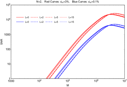
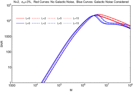
Figure 3: The SNR behavior of LISA with the change of the black hole mass $M$ at a distance $D_{L}=3\,\mathrm{Gpc},z=0.54$ with the angular number $l=2$. For each plot we have fixed the value of $N$ but change $L$. For the plot on the left, the galactic noise is not included and the red curves and blue curves correspond to the radiation efficiency $\epsilon_{rd}=3\%$ and $0.1\%$, respectively, while for the plot on the right we set $\epsilon_{rd}=3\%$, and the red curves denote the SNR without including the galactic noise and the blue curves denote the SNR affected by the galactic noise.

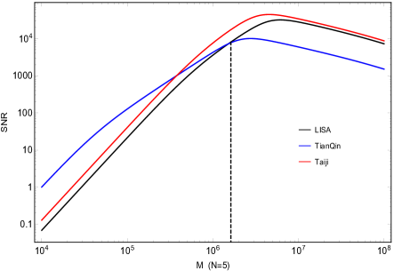
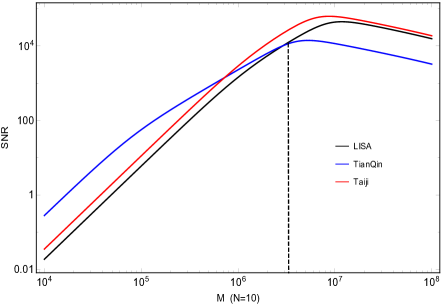
Figure 4: The comparison of SNR among LISA, TianQin and TaiJi with different black hole masses at a distance $D_{L}=3\,\mathrm{Gpc},z=0.54$ by taking the angular number $l=2$ and the radiation efficiency $\epsilon_{rd}=0.03$. In each plot we set $L=2$, and four different $N$ are designated correspondingly in the four plots.

In Fig. 4 we show a comparison of SNR among LISA, TianQin and TaiJi. From this figure one can see that there exists a maximal value of SNR for all these three detectors, and the mass related to the maximal SNR grows when the BHs deviate extensively from the Schwarzschild ones. It is clear to see that there exists a critical mass $M_{cri}$ in each plot. For the mass range $M<M_{cri}$, the SNR for TianQin is higher than LISA implying that TianQin is more sensitive to GWs emitted from BHs with comparatively smaller masses, while for more massive BHs with $M>M_{cri}$ the LISA and TaiJi is more sensitive for the detection. Different sensitivities of these three detectors were also reflected in the root sensitive curve shown in Fig. 1 which demonstrated that LISA and TaiJi are more sensitive to lower frequency (corresponding to bigger BHs) and TianQin is more sensitive to comparatively higher frequency GW signals (corresponding to smaller BHs). It is interesting to note that the critical mass $M_{cri}$ is related to the parameter $N$, which increases when the black hole deviates more from the standard Schwarzschild black hole. It is noticeable that in the whole frequency band (from low frequency to high frequency) the SNR of TaiJi is higher than LISA, which is consistent with the sensitivity demonstrated in Fig. 1. Comparing the values of $M_{cri}$ and the locations of the dominant mode peaks of SNR for different non-singular parameters, LISA and TaiJi are more promising to distinguish non-singular BHs from the standard Schwarzschild ones.

IV SNR for non-singular Bardeen BHs

IV.1 Quasinormal modes of Bardeen BHs

The metric of the non-singular Bardeen black hole is Bardeen

$$ds^{2}=-f(r)dt^{2}+\frac{1}{f(r)}dr^{2}+r^{2}(d\theta^{2}+\sin\theta^{2}d\phi^{2}),$$ (20)

where $f(r)$ is given by Bardeen

$$f(r)=1-\frac{2Mr^{2}}{(r^{2}+\beta^{2})^{\frac{3}{2}}}.$$ (21)

The parameter $\beta$ can be regarded as the charge of a self-gravitating magnetic monopole system with mass $M$. To ensure the existence of BHs, the parameter $\beta$ must be restricted to be $\beta^{2}\leq\frac{16}{27}M^{2}$ and one can clearly see that when $\beta=0$ the metric reduces to the Schwarzschild black hole. This parameter $\beta$ makes the spacetime non-singular, which leads to different dynamical behaviors of the gravitational perturbation in contrast to that of the Schwarzschild black hole.

The master equation for the axial gravitational perturbation was given by Ulhoa

$$\frac{d^{2}\phi}{dr_{\ast}^{2}}+\left[\omega^{2}-V(r)\right]\phi=0,$$ (22)

where the effective potential $V(r)$ reads

$$V(r)=f(r)\left(\frac{l(l+1)+2(f(r)-1)}{r^{2}}+\frac{1}{r}\frac{df(r)}{dr}+\frac{d^{2}f(r)}{dr^{2}}+2\kappa L\right),$$ (23)

in which $\kappa=8\pi$, and

$$L=\frac{3M}{|\beta|^{3}}\left(\frac{\sqrt{2\beta^{2}F}}{1+\sqrt{2\beta^{2}F}}\right)^{\frac{5}{2}},\qquad F=\frac{\beta^{2}}{2r^{4}}.$$ (24)

In Ulhoa the QNM was calculated by using the 3rd WKB method. It was found that compared with high order WKB approaches, the numerical result obtained by the 3rd WKB method is not very accurate Konoplya:2003ii . In order to distinguish this non-singular black hole from the Schwarzschild black hole, we need very accurate results of the QNM spectrum. Therefore, in our calculations we will employ the 13th order WKB method and the Pade approximation to guarantee the high precision in our numerical computation.

We list our result in Table. LABEL:table3. Analyzing the frequency of QNMs, we learn that with the increase of $\beta$, the real part of the QNM frequency increases for every fixed $l,n$ mode, while the imaginary part of the perturbation frequency decreases for any given $l>2$ with different $n$. Our result is different from that in Ulhoa , where it was claimed that the imaginary frequency keeps almost the same for different choices of $\beta$. This is because their 3rd WKB method is not accurate enough to show the details. Moreover in Ulhoa the behavior of QNMs with the change of the angular number $l$ is not discussed. With the Pade approximation, we are in a position to analyze carefully the dependence of the QNM frequency on the angular index $l$ and the overtone number $n$ until the limit $n\sim l$. With the increase of $l$ at the same overtone number $n$, we find that both the real part and the imaginary part monotonously increase for $\beta=0$ and $\beta=0.3$ in the condition $n\leq 2$ and $n\leq 1$, respectively. For bigger $\beta$, for example $\beta=0.6$, the imaginary part behaves differently. We have the spectrum of more accurate QNM frequencies for different modes. Hereafter we will focus on the calculation of single-mode SNR. For the complicated data, it is not easy to find the dominant mode in the gravitational perturbation. Here we will use again the criteria suggested in Wang:2004bv by examining min$\{\sqrt{\omega_{R}^{2}+\omega_{I}^{2}}\}$, which tells us that the mode $n=0,l=2$ is dominant in both the non-singular and the Schwarzschild BHs. Taking into account that the $n=0,l=2$ mode always has the strongest amplitude $\mathcal{A}_{lm}$, it gives us further confidence to employ the $n=0,l=2$ mode to calculate the SNR in our following discussion.

Table 4: QNMs frequency $M\omega$ for non-singular Bardeen BHs.

$l$	$n$	$\beta=0$	$\beta=0.3$	$\beta=0.6$
$2$	$0$	$0.373675-0.088964i$	$0.406175-0.087325i$	$0.553008-0.094534i$
	$1$	$0.346827-0.273931i$	$0.381988-0.269701i$	$0.525271-0.291523i$
	$2$	$0.299998-0.478098i$	$0.383018-0.475991i$	$0.435513-0.485159i$
$3$	$0$	$0.599443-0.092703i$	$0.626872-0.091561i$	$0.743159-0.089355i$
	$1$	$0.582644-0.281297i$	$0.612724-0.277584i$	$0.731708-0.268568i$
	$2$	$0.551686-0.479087i$	$0.586992-0.471962i$	$0.714495-0.445970i$
	$3$	$0.511943-0.690318i$	$0.692611-0.523967i$	$0.692336-0.618884i$
$4$	$0$	$0.809178-0.094163i$	$0.835574-0.093074i$	$0.942654-0.088437i$
	$1$	$0.796631-0.284334i$	$0.824486-0.280904i$	$0.934782-0.266149i$
	$2$	$0.772709-0.479908i$	$0.803399-0.473636i$	$0.919857-0.446242i$
	$3$	$0.739836-0.683924i$	$0.774487-0.673961i$	$0.899410-0.630009i$
	$4$	$0.701514-0.898237i$	$0.740946-0.883478i$	$0.876439-0.818826i$
$5$	$0$	$1.012295-0.094871i$	$1.039250-0.093792i$	$1.145670-0.088485i$
	$1$	$1.002221-0.285817i$	$1.030170-0.282482i$	$1.139280-0.266113i$
	$2$	$0.982695-0.480328i$	$1.012590-0.474430i$	$1.126900-0.445668i$
	$3$	$0.955004-0.680556i$	$0.987689-0.671579i$	$1.109250-0.628267i$
	$4$	$0.921081-0.888197i$	$0.957252-0.875455i$	$1.087490-0.814877i$
	$5$	$0.883335-1.104182i$	$0.923566-1.086900i$	$1.062670-1.005600i$

IV.2 SNR by LISA, TianQin and TaiJi

Following the discussion in Section III, here we are going to discuss the SNR of the GW signal to be detected by LISA for non-singular Bardeen BHs at first, and then we will make a comparison of SNR among different space GW detectors, such as LISA, TianQin and TaiJi. For the non-singular Bardeen black hole and the Schwarzschild black hole having the same dominant mode, it is easy to compare their single-mode SNR.

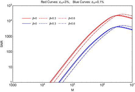
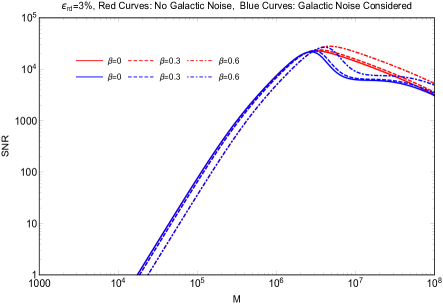
Figure 5: The SNR behavior of LISA with the change of the black hole mass $M$ at a distance $D_{L}=3\,\mathrm{Gpc},z=0.54$ when the angular index is taken $l=2$. For the left plot, the red curves and blue curves correspond to radiation efficiency $\epsilon_{rd}=3\%$ and $0.1\%$, respectively. For the right plot, we set $\epsilon_{rd}=3\%$ and consider the comparison between SNR affected by the galactic noise (marked by blue lines) and SNR without including the galactic noise (marked by red curves).

We show the SNR curves for the Bardeen BHs with three different values, $\beta=0,\beta=0.3$ and $\beta=0.6$ in Fig. 5. In the left panel we do not consider the galactic noise, while in the right panel the noise is included. The general property of the SNR in this case is quite similar to that reported above for the non-singular conformal BHs in Section III. When the black hole mass $M<2\times 10^{6}M_{\odot}$, the SNR for the Schwarzschild BHs with $\beta=0$ is higher than that of the non-singular Bardeen BHs with a non-zero $\beta$. However for more massive BHs, the SNR for the non-singular Bardeen black hole exhibits higher peaks for bigger $\beta$.

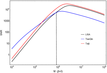
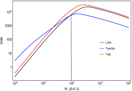
Figure 6: The comparison of SNR among LISA and TianQin and TaiJi for the Bardeen BHs.

In Fig. 6 we illustrate the comparison of SNR among LISA, TianQin and TaiJi. The comparison shows that there exists a critical mass $M_{cri}$, below which TianQin is more sensitive to detect the GW signal, while above this vaule LISA or TaiJi will detect the signal more sensitively. This critical mass $M_{cri}$ increases with the increase of the Bardeen factor $\beta$. In the whole frequency band, it is clear that TaiJi has higher SNR than LISA. Again comparing the values of $M_{cri}$ and the locations of SNR peaks for different Bardeen factors, LISA and TaiJi have more potential to distinguish the Bardeen non-singular BHs from the Schwarzschild ones.

V The uncertainty of parameter estimation

In last two sections we have calculated the SNR by detection of single mode GWs sourced by non-singular black holes. In this section, it is necessary to obtain the measurements errors of black holes parameters, such as mass $M$, conformal parameters $L,N$ and Bardeen parameter $\beta$. To this end, we are going to employ Fisher information matrix which is widely used to obtain the uncertainty in parameter estimation. In our calculation of Fisher matrix, we would like to follow the strategy presented in Ref. Cardoso .

V.1 Statistical Methods

We define the inner product between two signals $h_{1}(t)$ and $h_{2}(t)$ by Cardoso

$$(h_{1}|h_{2})=2\int_{0}^{\infty}\frac{\tilde{h}_{1}^{\ast}\tilde{h}_{2}+\tilde{h}_{2}^{\ast}\tilde{h}_{1}}{S_{N}(f)}df,$$ (25)

where the $S_{N}(f)$ is the noise spectral density for detetors, and $\tilde{h}_{1}(f)$ and $\tilde{h}_{2}(f)$ is the Fourier transform of the respective gravitational waveforms $h_{1}(t)$ and $h_{2}(t)$. With the definition of the inner product, the components of the Fisher matrix $\Gamma_{ab}$ are given by

$$\Gamma_{ab}=\left(\frac{\partial h}{\partial\theta^{a}}|\frac{\partial h}{\partial\theta^{b}}\right),$$ (26)

where the $\theta$ are a set of parameters that the gravitational waveforms depend on. In the large SNR limit, if the noise is stationary and Gaussian, the best-fit parameters will have a Gauss distribution centered on the correct values Cutler:1997ta . The probability that the GWs signal $s(t)$ is described by a set of given values of the source parameters $\theta^{a}$ is given by Cardoso

$$p(\boldsymbol{\theta}|s)=p^{(0)}(\boldsymbol{\theta})e^{-\frac{1}{2}\Gamma_{ab}\delta\theta^{a}\delta\theta^{b}},$$ (27)

where $\delta\theta^{a}=\theta^{a}-\hat{\theta}^{a}$ and $\hat{\theta}^{a}$ means the “true” values of the parameters, $p^{(0)}(\boldsymbol{\theta})$ stands for the distribution of the prior information. The uncertainty in the measurement of parameter $\theta^{a}$ is represented by the rms error $\Delta\theta^{a}=(\langle(\delta\theta^{a})^{2}\rangle)^{\frac{1}{2}}$ which can be calculated at large SNR by

$$\Delta\theta^{a}\approx\sqrt{(\Gamma^{-1})^{aa}}.$$ (28)

The gravitational waveforms considered in our calculation are

$$h_{+}(t) =A^{+}e^{-\pi f_{lmn}t/Q_{lmn}}\cos[2\pi f_{lmn}t+\phi^{+}_{lmn}]S_{lmn},$$ (29a)

$$h_{\times}(t) =A^{+}N_{\times}e^{-\pi f_{lmn}t/Q_{lmn}}\sin[2\pi f_{lmn}t+\phi^{\times}_{lmn}]S_{lmn},$$ (29b)

in which

$$A^{+}=\frac{M}{r}\mathcal{A}^{+}_{lmn},\quad A^{\times}=A^{+}N_{\times}=\frac{M}{r}\mathcal{A}^{\times}_{lmn},\quad\phi^{\times}_{lmn}=\phi^{+}_{lmn}+\phi^{0}_{lmn},$$ (30)

where $N_{\times}$ is some numerical factor. For simplicity, we assume that we know $N_{\times}$ and $\phi^{0}_{lmn}$ such that the waveform only depends on four parameters $(A^{+},\phi^{+}_{lmn},f_{lmn},Q_{lmn})$. Specifically, in Kerr case the four parameters can also be represented by $(A^{+},\phi^{+}_{lmn},M,j)$ because $f_{lmn}$ and $Q_{lmn}$ are only dependent on mass $M$ and angular momentum $j$. In black holes models found in alternative theories of gravity, the parameter basis could involve more parameters since we may need more parameters to describe $f_{lmn}$ and $Q_{lmn}$.

The parameter errors to leading order in $Q_{lmn}^{-1}$ in Kerr case have been analytically given in Ref. Cardoso

$$\sigma_{A^{+}}=\frac{\sqrt{2}A^{+}}{\rho_{FH}}\left|1+\frac{3\varpi}{8Q_{lmn}^{2}}\right|,$$ (31a)

$$\sigma_{\phi_{lmn}^{+}}=\frac{1}{\rho_{FH}}\left|1-\frac{\varpi}{4Q_{lmn}^{2}}\right|,$$ (31b)

$$\sigma_{M}=\frac{1}{\rho_{FH}}\left|\frac{2MQ_{lmn}f^{\prime}_{lmn}}{f_{lmn}Q^{\prime}_{lmn}}\left(1+\frac{1+4\varpi}{16Q_{lmn}^{2}}\right)\right|,$$ (31c)

$$\sigma_{j}=\frac{1}{\rho_{FH}}\left|\frac{2Q_{lmn}}{Q^{\prime}_{lmn}}\left(1+\frac{1+4\varpi}{16Q_{lmn}^{2}}\right)\right|,$$ (31d)

where

$$f^{\prime}_{lmn}=\frac{df_{lmn}}{dj},\quad Q^{\prime}_{lmn}=\frac{dQ_{lmn}}{dj},\quad\varpi=\frac{N_{\times}^{2}}{1+N_{\times}^{2}}\cos(2\phi^{\times}_{lmn})-\frac{1}{1+N_{\times}^{2}}\cos(2\phi^{+}_{lmn}).$$ (32)

It is apparently to note that Eq. (31) is also applicable to TianQin and TaiJi although these formulas are developed for LISA, since in Eq. (31) the SNR formula $\rho_{FH}$ is the unique factor related to characteristics of detector and this formula is valid to TianQin and TaiJi as we have discussed previously. For completeness, we show the numerical and analytical results of the mass errors to demonstrate the validity of the Eq. (31) for TianQin and TaiJi in Fig. 7 from which we can see that the numerical results are in good agreement with analytical results. In our calculation, as the choices made and explained in Ref. Cardoso , we also have assumed $N_{\times}=1,\phi^{\times}_{lmn}=\phi^{+}_{lmn}=0$, and $z=0.54,\epsilon_{ed}=3\%,D_{L}=3\mathrm{Gpc}$.

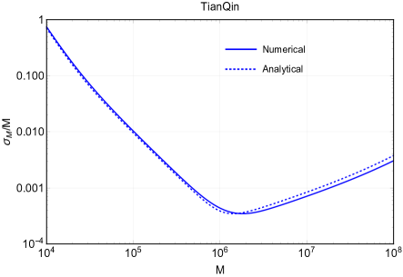
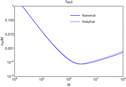
Figure 7: The mass error $\sigma_{M}/M$ for TianQin and TaiJi. The gravitational QNMs frequencies of Schwarzschild black holes used here are $l=2,n=0$ modes. The solid curves represent the numerical results and dotted curves stand for analytical results obtained by Eq. (31). One can see that the numerical and analytical results are in good agreement with each other. In our calculation, we have assumed $N_{\times}=1,\phi^{\times}_{lmn}=\phi^{+}_{lmn}=0$, and $z=0.54,\epsilon_{ed}=3\%,D_{L}=3\mathrm{Gpc}$.

V.2 Parameter Estimation Uncertainty of Non-Singular Black Holes

In this section, we numerically calculate the errors in the measurements of parameters for the non-singular black holes under the condition $N_{\times}=1,\phi^{\times}_{lmn}=\phi^{+}_{lmn}=0$, and $z=0.54,\epsilon_{ed}=3\%,D_{L}=3\mathrm{Gpc}$, as the condition we imposed in V.1. Note that the sensitivity curve of TaiJi behaves similarly to that of LISA, it is more interesting to compare the parameter detection errors between LISA and TianQin. The Bardeen black hole will be discussed firstly and then we move on to the discussion of conformal black hole.

V.2.1 Bardeen Black Hole Case

In Bardeen black hole case, we calculate Fisher matrix elements in the parameter basis $(A^{+},\phi^{+}_{lmn},M,\beta)$. However, mass $M$ and Bardeen parameter $\beta$ are not explicitly expressed in waveforms (29) where $f_{lmn}$ and $Q_{lmn}$ are present and they are dependent on the black hole parameter $M$ and $\beta$. The relations between $f_{lmn},Q_{lmn}$ and $M,\beta$ can not be analytically given. We overcome this problem by relating QNMs frequencies obtained numerically to black holes parameters with fitting formulas

$$f_{lmn} =\frac{\omega_{lmn}}{2\pi}=\frac{\mathcal{F}_{lmn}}{2\pi(1+z)M}=\frac{f_{1}+f_{2}(\beta_{max}-\beta)^{f_{3}}}{2\pi(1+z)M},$$ (33a)

$$Q_{lmn} =q_{1}+q_{2}(\beta_{max}-\beta)^{q_{3}},$$ (33b)

where $\beta_{max}=\frac{4}{3\sqrt{3}}$ is the maximum value of $\beta$, and

$$f_{1} =0.254409,\quad f_{2}=0.094561,\quad f_{3}=-0.656729,$$ (34a)

$$q_{1} =-0.238375,\quad q_{2}=2.187814,\quad q_{3}=-0.208734.$$ (34b)

After substituting Eq. (34) to waveforms (29), then the Fisher matrix can be obtained in the parameter basis $(A^{+},\phi^{+}_{lmn},M,\beta)$. Actually, we have used similar method in Section V.1 to estimate parameter errors and the fitting formulas and fitting coefficients are provided in Ref. Cardoso .

In Fig. 8 we show the dependence of parameter estimation errors for Bardeen parameter $\beta$ (denoted by $\sigma_{\beta}$) and black hole mass $M$ (denoted by $\sigma_{M}/M$) on the mass $M$ in the GWs detection by LISA (dashed lines) and TianQin (solid lines). The $\sigma_{\beta}$ curves are shown in the left panel from which we can see that with the increase of $\beta$ the errors $\sigma_{\beta}$ decrease. For both detectors, the curves behave in the same way as $\sigma_{\beta}$ decrease with the increase of $M$ until to some critical mass and then increase with the further increase of $M$, and the critical mass for TianQin is about $2\times 10^{6}M_{\odot}$ while for LISA it is about $4\times 10^{6}M_{\odot}$. In the higher frequency region (corresponding to $M\lesssim 10^{6}M_{\odot}$), $\sigma_{\beta}$ by LISA is bigger than that of TianQin, and the opposite result can be observed in the lower frequency band ($M\gtrsim 10^{6}M_{\odot}$). That is to say TianQin can detect parameter $\beta$ more precisely than LISA for relatively smaller black holes, while for more massive black holes, LISA can make a more precision detection. In the right panel, we show the mass error $\sigma_{M}/M$ which behaves generally similar to $\sigma_{\beta}$ but with two two different properties. The higher value of $\beta$ is related to a bigger mass error which is opposite to the behavior of $\sigma_{\beta}$. On the other hand, the differences of the value of $\sigma_{M}/M$ arising from the different $\beta$ will be reduced by increasing black hole mass. One can find that the errors in both panel become unacceptably large for mass $M\lesssim 10^{5}M_{\odot}$, but in general we can expect good detection accuracies for black hole mass $M\gtrsim 3\times 10^{5}M_{\odot}$ beyond which the errors are smaller than $0.01$. The best precision detections are provided by LISA for the black hole mass $M\approx 5\times 10^{6}M_{\odot}$ with both parameter errors $\sigma_{\beta}$ (when $\beta=0.6$) and $\sigma_{M}/M$ (when $\beta=0$) smaller than $10^{-4}$. Further more, we note that the characteristics of the behaviors of the errors curves can be reflected by the property of SNR $\rho_{FH}$, as the factor $\rho_{FH}^{-1}$ is present in the analytical expressions of errors in Eq. (31).

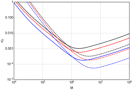
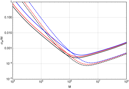
Figure 8: The dependence of parameter estimation errors for Bardeen parameter $\beta$ (left panel) and black hole mass $M$ (right panel) on the mass $M$. The black, red and blue curves correspond to $\beta=0,\beta=0.3$ and $\beta=0.6$, respectively. The dashed lines represent the parameter errors in the GWs detection by LISA and solid lines represent TianQin.

V.2.2 Conformal Black Hole Case

It was assumed in Ref. Toshmatov:2017kmw that the most natural non-singular black hole candidates from the numerous conformally invariant solutions are those which have less violation of the energy conditions. On the other hand, the QNMs frequencies can be approximated analytically when $N$ is large enough, and hence the fitting formulas relating black hole parameters to QNMs are not required. Therefore, it is necessary and interesting to estimate errors in parameters measurements at large $N$ limit. For the parameter space, we should point out that it would be more rigorous to include $N$ in the parameter space. However, as the less violation of the energy conditions for large $N$ Toshmatov:2017kmw but no limitations to parameter $L$ are implemented, we are more interested in exploring parameter $L$ and hence assuming a large value of $N$ is known. As a result, we do our calculation on the basis of parameter space $(A^{+},\phi^{+}_{lmn},M,L)$ which helps simplify our computation, and $N=100$ is assumed.

The effective potential Eq. (19) can also be written as Chen:2019iuo

$$V(r)=f(r)\left(\frac{l(l+1)}{r^{2}}-\frac{3}{r^{3}}+F_{1}(r)N+F_{2}(r)N^{2}\right),$$ (35)

where

$$F_{1}(r) =-\frac{2L^{2}(5r^{3}-6r^{2}+3L^{2}r-4L^{2})}{r^{3}(r^{2}+L^{2})^{2}}$$ (36)

$$F_{2}(r) =\frac{4L^{4}(r-1)}{r^{3}(r^{2}+L^{2})^{2}}.$$ (37)

In large $N$ limit, the effective potential can be approximated as

$$V(r)\approx f(r)F_{2}(r)N^{2}.$$ (38)

The approximation form of the potential suggests that we can use WKB approach to work out QNMs frequencies. In the calculation of QNMs frequencies, the 6th order WKB formula is given by Schutz ; PhysRevD.35.3621 ; Konoplya:2003ii

$$\frac{i(\omega^{2}-V_{m})}{\sqrt{-2V^{\prime\prime}_{m}}}-\sum_{i=2}^{6}\Lambda_{i}=n+\frac{1}{2},$$ (39)

where $m$ represents the quantities evaluated at the maximum (peak)of the potential, and we denote the location of the peak of potential as $r_{m}$ which can be obtained analytically. $V^{\prime\prime}_{m}$ denotes the value of the second order derivative of potential with respect to $r_{\ast}$ calculated at $r_{m}$. $\Lambda_{i}$ are higher order correction terms which can be ignored at large $N$ (or large $l$) limit and only the 1st order term is left, as in our current consideration. Based on 1st order WKB formula, the QNMs frequencies are given by

$$\omega\approx\sqrt{V_{m}}-i\left(n+\frac{1}{2}\right)\sqrt{-\frac{1}{2}\frac{V^{\prime\prime}_{m}}{V_{m}}}=N\sqrt{(fF_{2})_{m}}-i\left(n+\frac{1}{2}\right)\sqrt{-\frac{1}{2}\frac{(fF_{2})^{\prime\prime}_{m}}{(fF_{2})_{m}}}.$$ (40)

With the help of this expression of QNMS frequencies, we can get numerical elements of Fisher matrix and hence obtain parameter detection errors.

We show our results in Fig. 9 where the solid lines represent errors by TianQin and the dashed lines by LISA. The left panel shows the errors of parameter $L$. As expected, TianQin can make more precision detection of parameter in higher frequency band while for lower frequency region LISA is more sensitive. For a small value of $L=0.5$ (indicated by black lines), the value of $\sigma_{L}$ can be as low as $10^{-5}$ with black hole mass around $M\approx 10^{7}M_{\odot}$ suggesting that we can expect a great accuracy. While when we increase the value of $L$ to $L=4$ (red lines) and $L=10$ (blue lines), the value of $\sigma_{L}$ grows which means that the precision becomes worse. Therefore a smaller true value of $L$ will provide us a more accurate measurement. On the right panel, we show the detection errors of mass parameter. To get an accurate enough measurement of mass $M$ (say, errors smaller than $10^{-2}$), the critical mass value to reach this accuracy will become larger when increasing $L$. However, a larger $L$ can lead to a smaller minimum of errors at some certain large mass.

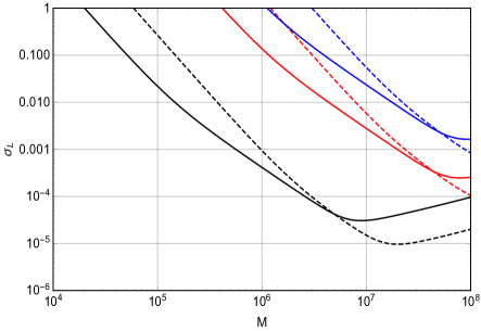
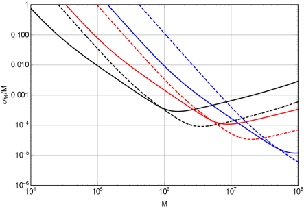
Figure 9: The behavior of parameter errors under the change of black hole mass. For both panels, solid lines correspond to errors by TianQin and dashed lines correspond to LISA. The left plot shows the behavior of $\sigma_{L}$ standing for the errors of parameter $L$ under different $L$ value, the black, red and blue lines correspond to $L=0.5,L=4$ and $L=10$, respectively. The right plot shows the errors of mass, in this case we take $L=0.2,L=0.5$ and $L=10$ which correspond to black, red and blue lines respectively.

VI Conclusions

In this paper we have calculated the quasinormal modes (QNMs) of the non-singular Bardeen BHs and singularity-free BHs in conformal gravity. We have also calculated their corresponding SNR in the single-mode waveform detection of GWs by the future space based interferometers, such as LISA, TianQin and TaiJi. We have found that the approximate formula (11) of SNR is not only valid for LISA, but also applicable to TianQin and TaiJi. Using this approach, we have calculated SNR for LISA, TianQin and TaiJi. We have investigated the impact of the conformal factor on the behavior of the SNR and found that the increase of the conformal factor will lead to a higher SNR for more massive BHs. For the Bardeen BHs, similar phenomena are also observed that a bigger Bardeen parameter $\beta$ will result in a higher SNR, when the Bardeen black hole is very massive. Once the black hole mass is $\sim 10^{6}M_{\odot}$, usually the GW perturbation in the Schwarzschild black hole has higher SNR. The signature of the non-singular modification will emerge when BHs become more massive. Comparing the SNRs among LISA, TianQin and TaiJi, we found that the SNR of TianQin is always higher than that of LISA and TaiJi when the black hole is not so massive. However for the black hole with mass over a critical mass, LISA and TaiJi will have stronger SNR compared to that of TianQin. Interestingly, this critical mass increases when the black hole deviates significantly from the Schwarzschild black hole. In our study, we have found that the effect of the galactic confusion noise is not negligible, and its influence on the Schwarzschild black hole appears when the black hole mass is a few times of $10^{6}M_{\odot}$, but for non-singular BHs the effect of the galactic noise will play an important role only for more massive holes. For the non-singular BHs, considering that their SNR peaks and dips appear for more massive BHs, it is expected that the LISA and TaiJi have more potential to distinguish them from the Schwarzschild black hole.

We have investigated the errors in parameter estimation for non-singular black holes by TianQin and LISA, and find that the analytical formulas of errors developed in Ref. Cardoso for LISA can also be applied to TianQin and TaiJi. As expected, TianQin can make more precise detection than LISA for smaller black holes (higher frequency), while in larger black holes regime (lower frequency) the more accurate measurements of parameters are provided by LISA. In the detection of Bardeen parameter $\beta$, we find that a higher true value of $\beta$ will result in a more precision detection, but the mass detection accuracy will become worse. In the detection of parameter $L$ for conformal black holes, it is found that a smaller value of $L$ is favored in the sense that higher values of $L$ correspond to less accurate detection. In general, in the detection of parameters for both non-singular black holes, our results suggest that we can expect good accuracy in the future GWs detections by TianQin and LISA, as well as TaiJi. Therefore, it is promising to explore the non-singular black holes with the future space-based detectors.

We have only studied the SNR for the single mode detection in this paper, and it is worth extending the discussion to multi-mode detections and making parameter estimation (rather than just estimation errors) with the detected ringdown signals. For the multi-mode discussion, we have provided very accurate QNM frequency samples, which contain important properties for non-singular BHs. Besides we have only concentrated on BHs without angular momenta. Considering that BHs with rotation are more realistic in the universe, so it would be very interesting to generalize our investigations to probe QNMs and SNR for rotating non-singular BHs.

Appendix A The approximation formula of SNR for TianQin and TaiJi

Although the approximate formula of SNR given by Eq. (11) from Ref. Cardoso was mainly developed in the context of LISA and the process of deriving Eq. (11) is dependent on the detector characteristics, the authors in Ref. Cardoso claimed that the expressions used in the derivation are valid for any interferometric detectors. To prove this claim, we calculate the SNR by using Eq. (11) for four QNMs in the Kerr BHs with $(l,m)=\{(2,1),(2,2),(3,3),(4,4)\}$ considered in Ref. Shi , and compare the SNR of TianQin and TaiJi calculated by doing the full integral with the formula of SNR, given by Eq. (6a).

Table 5: Fitting coefficients given by Ref. Cardoso

$(l,m)$	$f_{1}(l,m)$	$f_{2}(l,m)$	$f_{3}(l,m)$	$q_{1}(l,m)$	$q_{2}(l,m)$	$q_{3}(l,m)$
$(2,1)$	$0.6000$	$-0.2339$	$0.4175$	$-0.3000$	$2.3561$	$-0.2277$
$(2,2)$	$1.5251$	$-1.1568$	$0.1292$	$0.7000$	$1.4187$	$-0.4990$
$(3,3)$	$1.8956$	$-1.3043$	$0.1818$	$0.9000$	$2.3430$	$-0.4810$
$(4,4)$	$2.3000$	$-1.5056$	$0.2244$	$1.1929$	$3.1191$	$-0.4825$

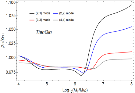
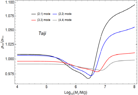
Figure 10: The SNR ratio of $\rho_{\mathrm{int}}$ to $\rho_{FH}$. In this plot we take $\chi_{f}=0.76$, $\chi_{eff}=0.3$, $\nu=2/9$ and luminosity distance $r=15\mathrm{Gpc}$.

The fitting formulae of the oscillation frequency $\omega_{lm}$ and damping time $\tau_{lm}$ for the remnant Kerr black hole with the redshifted mass $M_{z}=(1+z)M$ are given by Cardoso

$$\omega_{lm} =\frac{f_{1}(l,m)+f_{2}(l,m)(1-\chi_{f})^{f_{3}(l,m)}}{M_{z}},$$ (41a)

$$\tau_{lm} =\frac{2(q_{1}(l,m)+q_{2}(l,m)(1-\chi_{f})^{q_{3}(l,m)}}{\omega_{lm}},$$ (41b)

where $\chi_{f}$ is the final spin parameter and the fitting coefficients are listed in Table. LABEL:table4. The amplitudes $\mathcal{A}_{lm}^{+}=\mathcal{A}_{lm}^{\times}=\mathcal{A}_{lm}$ are given by Kamaretsos ; Meidam

$$\mathcal{A}_{22}(\nu) =0.864\nu,$$ (42a)

$$\mathcal{A}_{21}(\nu) =0.43(\sqrt{1-4\nu}-\chi_{eff})\mathcal{A}_{22}(\nu),$$ (42b)

$$\mathcal{A}_{33}(\nu) =0.44(1-4\nu)^{0.45}\mathcal{A}_{22}(\nu),$$ (42c)

$$\mathcal{A}_{44}(\nu) =(5.4(\nu-0.22)^{2}+0.04)\mathcal{A}_{22}(\nu),$$ (42d)

and

$$\nu=\frac{m_{1}m_{2}}{(m_{1}+m_{2})^{2}},$$ (43)

$$\chi_{eff}=\frac{1}{2}\left(\sqrt{1-4\nu}\chi_{1}+\frac{m_{1}\chi_{1}-m_{2}\chi_{2}}{m_{1}+m_{2}}\right),$$ (44)

where $(m_{1},m_{2})$ are the masses and $(\chi_{1},\chi_{2})$ are the spin parameters of the original BHs. The energy radiation efficiency $\epsilon_{rd}$ appeared in Eq. (11) is related to the amplitude $\mathcal{A}_{lm}$ by Cardoso

$$\mathcal{A}_{lm}=\sqrt{\frac{32Q_{lm}\epsilon_{rd}}{Mf_{lm}(1+4Q_{lm}^{2})}}.$$ (45)

We have omitted the overtone index $n$ in our expressions because only $n=0$ modes are considered here. The SNR obtained by Eq. (6a) is denoted by $\rho_{\mathrm{int}}$,

$$\rho_{\mathrm{int}}^{2}=4\int_{f_{low}}^{f_{high}}\frac{|\tilde{h}_{+}|^{2}+|\tilde{h}_{\times}|^{2}}{S_{n}(f)}df,$$ (46)

where $f_{low}$ is taken to be the half of the $(2,1)$ mode oscillation frequency and $f_{high}$ is taken to be two times of the $(4,4)$ mode frequency, and we also take the angle average $<|S_{lm}|^{2}>=1/4\pi$ for all modes following the average made in Ref. Cardoso . Now we have calculated $\rho_{FH}$ by adopting the approximate formula Eq. (11) and $\rho_{\mathrm{int}}$ obtained from the direct integral (A5) for comparison. In Fig. 10 we show the behavior of the ratio $\rho_{\mathrm{int}}/\rho_{FH}$ with the change of the black hole redshifted mass $M_{z}$ for four different single QNMs. This figure shows that the value of $\rho_{\mathrm{int}}$ is close to $\rho_{FH}$, which suggests that the approximate formula Eq. (11) we have applied to calculate SNR for TianQin and TaiJi is feasible with acceptable errors in a single-mode wave detection.

References

- (1) LIGO Scientific, Virgo collaboration, B. Abbott et al., GWTC-1: A Gravitational-Wave Transient Catalog of Compact Binary Mergers Observed by LIGO and Virgo during the First and Second Observing Runs, Phys. Rev. X 9 (2019) 031040, [1811.12907].
- (2) LIGO Scientific, Virgo collaboration, B. P. Abbott et al., Observation of Gravitational Waves from a Binary Black Hole Merger, Phys. Rev. Lett. 116 (2016) 061102.
- (3) LIGO Scientific, Virgo collaboration, R. Abbott et al., GWTC-2: Compact Binary Coalescences Observed by LIGO and Virgo During the First Half of the Third Observing Run, 2010.14527.
- (4) Y. Michimura, T. Fujita, S. Morisaki, H. Nakatsuka and I. Obata, Ultralight Vector Dark Matter Search with Auxiliary Length Channels of Gravitational Wave Detectors, 2008.02482.
- (5) W. DeRocco and A. Hook, Axion interferometry, Phys. Rev. D 98 (2018) 035021, [1802.07273].
- (6) I. Obata, T. Fujita and Y. Michimura, Optical Ring Cavity Search for Axion Dark Matter, Phys. Rev. Lett. 121 (2018) 161301, [1805.11753].
- (7) H. Liu, B. D. Elwood, M. Evans and J. Thaler, Searching for Axion Dark Matter with Birefringent Cavities, Phys. Rev. D 100 (2019) 023548, [1809.01656].
- (8) K. Nagano, T. Fujita, Y. Michimura and I. Obata, Axion Dark Matter Search with Interferometric Gravitational Wave Detectors, Phys. Rev. Lett. 123 (2019) 111301, [1903.02017].
- (9) D. Martynov and H. Miao, Quantum-enhanced interferometry for axion searches, Phys. Rev. D 101 (2020) 095034, [1911.00429].
- (10) H. Grote and Y. Stadnik, Novel signatures of dark matter in laser-interferometric gravitational-wave detectors, Phys. Rev. Res. 1 (2019) 033187, [1906.06193].
- (11) S. Morisaki and T. Suyama, Detectability of ultralight scalar field dark matter with gravitational-wave detectors, Phys. Rev. D 100 (2019) 123512, [1811.05003].
- (12) A. Pierce, K. Riles and Y. Zhao, Searching for Dark Photon Dark Matter with Gravitational Wave Detectors, Phys. Rev. Lett. 121 (2018) 061102, [1801.10161].
- (13) J. Manley, M. D. Chowdhury, D. Grin, S. Singh and D. J. Wilson, Searching for vector dark matter with an optomechanical accelerometer, 2007.04899.
- (14) Z. J. Weiner, P. Adshead and J. T. Giblin, Constraining early dark energy with gravitational waves before recombination, 2008.01732.
- (15) A. Garoffolo, M. Raveri, A. Silvestri, G. Tasinato, C. Carbone, D. Bertacca et al., Detecting Dark Energy Fluctuations with Gravitational Waves, 2007.13722.
- (16) A. Singh, Dark energy gravitational wave observations and ice age periodicity, Phys. Lett. B 802 (2020) 135226, [2002.07037].
- (17) J. Noller, Cosmological constraints on dark energy in light of gravitational wave bounds, Phys. Rev. D 101 (2020) 063524, [2001.05469].
- (18) W. Yang, S. Pan, D. F. Mota and M. Du, Forecast constraints on Anisotropic Stress in Dark Energy using gravitational-waves, 2001.02180.
- (19) H.-L. Li, D.-Z. He, J.-F. Zhang and X. Zhang, Quantifying the impacts of future gravitational-wave data on constraining interacting dark energy, JCAP 06 (2020) 038, [1908.03098].
- (20) J.-F. Zhang, H.-Y. Dong, J.-Z. Qi and X. Zhang, Prospect for constraining holographic dark energy with gravitational wave standard sirens from the Einstein Telescope, Eur. Phys. J. C 80 (2020) 217, [1906.07504].
- (21) S.-J. Jin, D.-Z. He, Y. Xu, J.-F. Zhang and X. Zhang, Forecast for cosmological parameter estimation with gravitational-wave standard siren observation from the Cosmic Explorer, JCAP 03 (2020) 051, [2001.05393].
- (22) Z.-W. Zhao, L.-F. Wang, J.-F. Zhang and X. Zhang, Prospects for improving cosmological parameter estimation with gravitational-wave standard sirens from Taiji, Sci. Bull. 65 (2020) 1340–1348, [1912.11629].
- (23) T.-J. Zhang, Y. Liu, Z.-E. Liu, H.-Y. Wan, T.-T. Zhang and B.-Q. Wang, The constraint ability of Hubble parameter by gravitational wave standard sirens on cosmological parameters, Eur. Phys. J. C 79 (2019) 900, [1910.11157].
- (24) J.-F. Zhang, M. Zhang, S.-J. Jin, J.-Z. Qi and X. Zhang, Cosmological parameter estimation with future gravitational wave standard siren observation from the Einstein Telescope, JCAP 09 (2019) 068, [1907.03238].
- (25) L.-F. Wang, Z.-W. Zhao, J.-F. Zhang and X. Zhang, A preliminary forecast for cosmological parameter estimation with gravitational-wave standard sirens from TianQin, 1907.01838.
- (26) X. Zhang, Gravitational wave standard sirens and cosmological parameter measurement, Sci. China Phys. Mech. Astron. 62 (2019) 110431, [1905.11122].
- (27) R. C. Nunes, Searching for modified gravity in the astrophysical gravitational wave background: Application to ground-based interferometers, Phys. Rev. D 102 (2020) 024071, [2007.07750].
- (28) S. Mastrogiovanni, D. Steer and M. Barsuglia, Probing modified gravity theories and cosmology using gravitational-waves and associated electromagnetic counterparts, Phys. Rev. D 102 (2020) 044009, [2004.01632].
- (29) R. Niu, X. Zhang, T. Liu, J. Yu, B. Wang and W. Zhao, Constraining Screened Modified Gravity by Space-borne Gravitational-wave Detectors, Astrophys. J. 890 (10, 2019) 163, [1910.10592].
- (30) S. Ma and N. Yunes, Improved Constraints on Modified Gravity with Eccentric Gravitational Waves, Phys. Rev. D 100 (2019) 124032, [1908.07089].
- (31) J. Kormendy and D. Richstone, Inward bound—the search for supermassive black holes in galactic nuclei, Annual Review of Astronomy and Astrophysics 33 (1995) 581.
- (32) Y.-M. Hu, J. Mei and J. Luo, Science prospects for space-borne gravitational-wave missions, National Science Review 4 (2017) 683.
- (33) E. Barausse, J. Bellovary, E. Berti, K. Holley-Bockelmann, B. Farris, B. Sathyaprakash et al., Massive Black Hole Science with eLISA, J. Phys. Conf. Ser. 610 (2015) 012001.
- (34) A. Klein et al., Science with the space-based interferometer eLISA: Supermassive black hole binaries, Phys. Rev. D93 (2016) 024003.
- (35) GRAVITY collaboration, R. Abuter et al., Detection of the gravitational redshift in the orbit of the star S2 near the Galactic centre massive black hole, Astron. Astrophys. 615 (2018) L15.
- (36) P. Amaro-Seoane, H. Audley, S. Babak, J. Baker, E. Barausse, P. Bender et al., Laser interferometer space antenna, arXiv:1702.00786 [astro-ph.IM] (2017) .
- (37) W.-R. Hu and Y.-L. Wu, The Taiji Program in Space for gravitational wave physics and the nature of gravity, Natl. Sci. Rev. 4 (2017) 685–686.
- (38) J. Luo, L.-S. Chen, H.-Z. Duan, Y.-G. Gong, S. Hu, J. Ji et al., TianQin: a space-borne gravitational wave detector, Classical and Quantum Gravity 33 (2016) 035010.
- (39) LIGO Scientific, Virgo collaboration, B. P. Abbott et al., GW170817: Observation of Gravitational Waves from a Binary Neutron Star Inspiral, Phys. Rev. Lett. 119 (2017) 161101.
- (40) LIGO Scientific, Virgo, Fermi-GBM, INTEGRAL collaboration, B. P. Abbott et al., Gravitational Waves and Gamma-rays from a Binary Neutron Star Merger: GW170817 and GRB 170817A, Astrophys. J. 848 (2017) L13.
- (41) A. Goldstein et al., An Ordinary Short Gamma-Ray Burst with Extraordinary Implications: Fermi-GBM Detection of GRB 170817A, Astrophys. J. 848 (2017) L14.
- (42) I. Arcavi et al., Optical emission from a kilonova following a gravitational-wave-detected neutron-star merger, Nature 551 (2017) 64.
- (43) D. A. Coulter et al., Swope Supernova Survey 2017a (SSS17a), the Optical Counterpart to a Gravitational Wave Source, Science (2017) .
- (44) V. M. Lipunov et al., MASTER Optical Detection of the First LIGO/Virgo Neutron Star Binary Merger GW170817, Astrophys. J. 850 (2017) L1.
- (45) DES, Dark Energy Camera GW-EM collaboration, M. Soares-Santos et al., The Electromagnetic Counterpart of the Binary Neutron Star Merger LIGO/Virgo GW170817. I. Discovery of the Optical Counterpart Using the Dark Energy Camera, Astrophys. J. 848 (2017) L16.
- (46) N. R. Tanvir et al., The Emergence of a Lanthanide-Rich Kilonova Following the Merger of Two Neutron Stars, Astrophys. J. 848 (2017) L27.
- (47) S. Valenti, D. J. Sand, S. Yang, E. Cappellaro, L. Tartaglia, A. Corsi et al., The discovery of the electromagnetic counterpart of GW170817: kilonova AT 2017gfo/DLT17ck, Astrophys. J. 848 (2017) L24.
- (48) LIGO Scientific, Virgo collaboration, B. Abbott et al., GW190425: Observation of a Compact Binary Coalescence with Total Mass , Astrophys. J. Lett. 892 (2020) L3, [2001.01761].
- (49) A. Chen, N. K. Johnson-McDaniel, T. Dietrich and R. Dudi, Distinguishing high-mass binary neutron stars from binary black holes with second- and third-generation gravitational wave observatories, 2001.11470.
- (50) M. Shibata and K. Hotokezaka, Merger and Mass Ejection of Neutron-Star Binaries, Ann. Rev. Nucl. Part. Sci. 69 (2019) 41–64.
- (51) M. W. Coughlin, T. Dietrich, B. Margalit and B. D. Metzger, Multimessenger Bayesian parameter inference of a binary neutron star merger, Mon. Not. Roy. Astron. Soc. 489 (2019) L91–L96.
- (52) K. Kiuchi, K. Kyutoku, M. Shibata and K. Taniguchi, Revisiting the lower bound on tidal deformability derived by AT 2017gfo, Astrophys. J. 876 (2019) L31.
- (53) E. E. Flanagan and T. Hinderer, Constraining neutron star tidal Love numbers with gravitational wave detectors, Phys. Rev. D77 (2008) 021502.
- (54) V. Cardoso, E. Franzin and P. Pani, Is the gravitational-wave ringdown a probe of the event horizon?, Phys. Rev. Lett. 116 (2016) 171101[Erratum: Phys. Rev. Lett.117,no.8,089902(2016)].
- (55) V. Cardoso, S. Hopper, C. F. B. Macedo, C. Palenzuela and P. Pani, Gravitational-wave signatures of exotic compact objects and of quantum corrections at the horizon scale, Phys. Rev. D94 (2016) 084031.
- (56) J. Abedi, H. Dykaar and N. Afshordi, Echoes from the Abyss: Tentative evidence for Planck-scale structure at black hole horizons, Phys. Rev. D96 (2017) 082004.
- (57) J. Westerweck, A. Nielsen, O. Fischer-Birnholtz, M. Cabero, C. Capano, T. Dent et al., Low significance of evidence for black hole echoes in gravitational wave data, Phys. Rev. D 97 (2018) 124037, [1712.09966].
- (58) K. W. Tsang, A. Ghosh, A. Samajdar, K. Chatziioannou, S. Mastrogiovanni, M. Agathos et al., A morphology-independent search for gravitational wave echoes in data from the first and second observing runs of Advanced LIGO and Advanced Virgo, Phys. Rev. D 101 (2020) 064012, [1906.11168].
- (59) LIGO Scientific, Virgo collaboration, B. P. Abbott et al., GW151226: Observation of Gravitational Waves from a 22-Solar-Mass Binary Black Hole Coalescence, Phys. Rev. Lett. 116 (2016) 241103.
- (60) LIGO Scientific, Virgo collaboration, B. P. Abbott et al., GW170608: Observation of a 19-solar-mass Binary Black Hole Coalescence, Astrophys. J. 851 (2017) L35.
- (61) LIGO Scientific, Virgo collaboration, B. P. Abbott et al., GW170814: A Three-Detector Observation of Gravitational Waves from a Binary Black Hole Coalescence, Phys. Rev. Lett. 119 (2017) 141101.
- (62) LIGO Scientific, Virgo collaboration, B. P. Abbott et al., Binary Black Hole Mergers in the first Advanced LIGO Observing Run, Phys. Rev. X6 (2016) 041015[erratum: Phys. Rev.X8,no.3,039903(2018)].
- (63) LIGO Scientific, VIRGO collaboration, B. P. Abbott et al., GW170104: Observation of a 50-Solar-Mass Binary Black Hole Coalescence at Redshift 0.2, Phys. Rev. Lett. 118 (2017) 221101[Erratum: Phys. Rev. Lett.121,no.12,129901(2018)].
- (64) A. Ashtekar and M. Bojowald, Quantum geometry and the Schwarzschild singularity, Class. Quant. Grav. 23 (2006) 391–411.
- (65) P. Nicolini, A. Smailagic and E. Spallucci, Noncommutative geometry inspired Schwarzschild black hole, Phys. Lett. B632 (2006) 547–551.
- (66) J. C. Lopez-Dominguez, O. Obregon, M. Sabido and C. Ramirez, Towards Noncommutative Quantum Black Holes, Phys. Rev. D74 (2006) 084024.
- (67) S. Hossenfelder, L. Modesto and I. Premont-Schwarz, A Model for non-singular black hole collapse and evaporation, Phys. Rev. D81 (2010) 044036.
- (68) M. Bojowald, S. Brahma and D.-h. Yeom, Effective line elements and black-hole models in canonical loop quantum gravity, Phys. Rev. D98 (2018) 046015.
- (69) A. Ashtekar, J. Olmedo and P. Singh, Quantum Transfiguration of Kruskal Black Holes, Phys. Rev. Lett. 121 (2018) 241301.
- (70) A. Ashtekar, J. Olmedo and P. Singh, Quantum extension of the Kruskal spacetime, Phys. Rev. D98 (2018) 126003.
- (71) N. Bodendorfer, F. M. Mele and J. Münch, Effective Quantum Extended Spacetime of Polymer Schwarzschild Black Hole, Class. Quant. Grav. 36 (2019) 195015.
- (72) A. Ashtekar, Black Hole evaporation: A Perspective from Loop Quantum Gravity, Universe 6 (2020) 21.
- (73) K. Jusufi, M. Jamil, H. Chakrabarty, Q. Wu, C. Bambi and A. Wang, Rotating regular black holes in conformal massive gravity, 1911.07520.
- (74) J. Ben Achour, F. Lamy, H. Liu and K. Noui, Polymer Schwarzschild black hole: An effective metric, EPL 123 (2018) 20006, [1803.01152].
- (75) J. Ben Achour, S. Brahma and J.-P. Uzan, Bouncing compact objects. Part I. Quantum extension of the Oppenheimer-Snyder collapse, JCAP 03 (2020) 041, [2001.06148].
- (76) J. Ben Achour and J.-P. Uzan, Bouncing compact objects II: Effective theory of a pulsating Planck star, 2001.06153.
- (77) S. Capozziello and M. De Laurentis, Extended Theories of Gravity, Phys. Rept. 509 (2011) 167–321.
- (78) E. Ayon-Beato and A. Garcia, Regular black hole in general relativity coupled to nonlinear electrodynamics, Phys. Rev. Lett. 80 (1998) 5056–5059.
- (79) F. Englert, C. Truffin and R. Gastmans, Conformal Invariance in Quantum Gravity, Nucl. Phys. B117 (1976) 407.
- (80) G. ’t Hooft, A class of elementary particle models without any adjustable real parameters, Found. Phys. 41 (2011) 1829–1856.
- (81) M. P. Dabrowski, J. Garecki and D. B. Blaschke, Conformal transformations and conformal invariance in gravitation, Annalen Phys. 18 (2009) 13–32.
- (82) P. D. Mannheim, Making the Case for Conformal Gravity, Found. Phys. 42 (2012) 388–420.
- (83) P. D. Mannheim, Mass Generation, the Cosmological Constant Problem, Conformal Symmetry, and the Higgs Boson, Prog. Part. Nucl. Phys. 94 (2017) 125–183.
- (84) L. Modesto and L. Rachwal, Finite Conformal Quantum Gravity and Nonsingular Spacetimes, arXiv:1605.04173 [hep-th] (2016) .
- (85) C. Bambi, L. Modesto and L. Rachwał, Spacetime completeness of non-singular black holes in conformal gravity, JCAP 1705 (2017) 003.
- (86) R. A. Konoplya and A. Zhidenko, Quasinormal modes of black holes: From astrophysics to string theory, Rev. Mod. Phys. 83 (2011) 793–836.
- (87) J. Matyjasek and M. Opala, Quasinormal modes of black holes. The improved semianalytic approach, Phys. Rev. D96 (2017) 024011.
- (88) R. A. Konoplya, A. Zhidenko and A. F. Zinhailo, Higher order WKB formula for quasinormal modes and grey-body factors: recipes for quick and accurate calculations, Class. Quant. Grav. 36 (2019) 155002.
- (89) E. Berti, V. Cardoso and C. M. Will, Gravitational-wave spectroscopy of massive black holes with the space interferometer LISA, Phys. Rev. D 73 (Mar, 2006) 064030.
- (90) E. Berti, V. Cardoso and A. O. Starinets, Quasinormal modes of black holes and black branes, Class. Quant. Grav. 26 (2009) 163001.
- (91) S.A.Teukolsky, Pertubations of a rotation black hole.II. Dynamical stability of the kerr metric, Astrophys.J. 185 (1973) 635.
- (92) T. Robson, N. J. Cornish and C. Liug, The construction and use of LISA sensitivity curves, Class. Quant. Grav. 36 (2019) 105011.
- (93) S. L. Larson, W. A. Hiscock and R. W. Hellings, Sensitivity curves for spaceborne gravitational wave interferometers, Phys. Rev. D 62 (2000) 062001.
- (94) D. Liang, Y. Gong, A. J. Weinstein, C. Zhang and C. Zhang, Frequency response of space-based interferometric gravitational-wave detectors, Phys. Rev. D99 (2019) .
- (95) E. E. Flanagan and S. A. Hughes, Measuring gravitational waves from binary black hole coalescences: 1. Signal-to-noise for inspiral, merger, and ringdown, Phys. Rev. D57 (1998) 4535–4565.
- (96) N. J. Cornish and S. L. Larson, Space missions to detect the cosmic gravitational wave background, Class. Quant. Grav. 18 (2001) 3473.
- (97) N. Cornish and T. Robson, Galactic binary science with the new LISA design, Journal of Physics: Conference Series 840 (2017) 012024.
- (98) C. Bambi, L. Modesto and L. Rachwał, Spacetime completeness of non-singular black holes in conformal gravity, JCAP 1705 (2017) 003.
- (99) C.-Y. Chen and P. Chen, Gravitational perturbations of nonsingular black holes in conformal gravity, Phys. Rev.D 99 (2019) 104003.
- (100) S. Iyer and C. M. Will, Black Hole Normal Modes: A WKB Approach. 1. Foundations and Application of a Higher Order WKB Analysis of Potential Barrier Scattering, Phys. Rev. D35 (1987) .
- (101) B. Wang, C.-Y. Lin and C. Molina, Quasinormal behavior of massless scalar field perturbation in Reissner-Nordstrom anti-de Sitter spacetimes, Phys. Rev. D70 (2004) 064025.
- (102) U. Sperhake, B. J. Kelly, P. Laguna, K. L. Smith and E. Schnetter, Black hole head-on collisions and gravitational waves with fixed mesh-refinement and dynamic singularity excision, Phys. Rev. D 71 (2005) 124042, [gr-qc/0503071].
- (103) J. Bardeen, Proceedings of GR5, Tiflis, U.S.S.R., 1968.
- (104) S. C. Ulhoa, On Quasinormal Modes for Gravitational Perturbations of Bardeen Black Hole, Braz. J. Phys. 44 (2014) 380.
- (105) R. A. Konoplya, Quasinormal behavior of the d-dimensional Schwarzschild black hole and higher order WKB approach, Phys. Rev. D68 (2003) 024018.
- (106) C. Cutler, Angular resolution of the LISA gravitational wave detector, Phys. Rev. D 57 (1998) 7089–7102, [gr-qc/9703068].
- (107) B. Toshmatov, C. Bambi, B. Ahmedov, A. Abdujabbarov and Z. e. Stuchlík, Energy conditions of non-singular black hole spacetimes in conformal gravity, Eur. Phys. J. C 77 (2017) 542, [1702.06855].
- (108) B. Schutz and C.M.Will, Black hole normal modes - a semianalytic approach, Astrophysical Journal 291 (1985) L33.
- (109) S. Iyer and C. M. Will, Black-hole normal modes: A wkb approach. i. foundations and application of a higher-order wkb analysis of potential-barrier scattering, Phys. Rev. D 35 (Jun, 1987) 3621–3631.
- (110) C. Shi, J. Bao, H.-T. Wang, J.-d. Zhang, Y.-M. Hu, A. Sesana et al., Science with the tianqin observatory: Preliminary results on testing the no-hair theorem with ringdown signals, Phys. Rev. D 100 (2019) 044036.
- (111) I. Kamaretsos, M. Hannam and B. S. Sathyaprakash, Is black-hole ringdown a memory of its progenitor?, Phys. Rev. Lett. 109 (2012) 141102.
- (112) J. Meidam, M. Agathos, C. Van Den Broeck, J. Veitch and B. S. Sathyaprakash, Testing the no-hair theorem with black hole ringdowns using tiger, Phys. Rev. D 90 (2014) 064009.