Coronal Dimming as a Proxy for Stellar Coronal Mass Ejections
Abstract
Solar coronal dimmings have been observed extensively in the past two decades and are believed to have close association with coronal mass ejections (CMEs). Recent study found that coronal dimming is the only signature that could differentiate powerful flares that have CMEs from those that do not. Therefore, dimming might be one of the best candidates to observe the stellar CMEs on distant Sun-like stars. In this study, we investigate the possibility of using coronal dimming as a proxy to diagnose stellar CMEs. By simulating a realistic solar CME event and corresponding coronal dimming using a global magnetohydrodynamics model (AWSoM: Alfvén-wave Solar Model), we first demonstrate the capability of the model to reproduce solar observations. We then extend the model for simulating stellar CMEs by modifying the input magnetic flux density as well as the initial magnetic energy of the CME flux rope. Our result suggests that with improved instrument sensitivity, it is possible to detect the coronal dimming signals induced by the stellar CMEs.
keywords:
magnetohydrodynamics (MHD) – methods: numerical – solar wind – Sun: corona – Sun: coronal mass ejections (CMEs)1 Introduction
“Coronal dimming” refers as the reduction in intensity on or near the solar disk across a large area during solar eruptive events. It was first observed in white light corona and described as a “depletion” (Hansen et al., 1974) and later was found in solar X-ray observations as “transient coronal holes” (Rust & Hildner, 1976). The studies about coronal dimming dramatically increased with Solar and Heliospheric Observatory (SOHO)/Extreme-ultraviolet Imaging (EIT) observations (Delaboudinière et al., 1995), with which the coronal dimming was first observed in multiple EUV channels with different emission temperatures (Thompson et al., 1998). The coronal dimming was also found usually associated with coronal EUV waves (also called “EIT waves”, Thompson et al. 1999). Recently, with EUV observations of unprecedented high temporal (12 s) and spatial resolution (0.6 arcsec) in seven channels from Solar Dynamics Observatory (SDO; Pesnell et al. 2012)/Atmospheric Imaging Assembly (AIA; Lemen et al. 2012) as well as the high spectral resolution data from SDO/Extreme Ultraviolet Variability Experiment (EVE; Woods et al. 2012), it provides us an unique opportunity for in-depth studies about coronal dimming.
Two decades of solar observations suggest that all coronal dimmings are associated with coronal mass ejections (CMEs; e.g., Sterling & Hudson 1997; Reinard & Biesecker 2008). Furthermore, since observations show simultaneous and co-spatial dimming in multiple coronal lines (e.g., Zarro et al. 1999; Sterling et al. 2000) and the spectroscopic observations show that the dimming region has up-flowing expanding plasma (e.g., Harra & Sterling 2001; Harra et al. 2007; Imada et al. 2007; Jin et al. 2009; Attrill et al. 2010; Tian et al. 2012), it is widely accepted that the coronal dimming is due to the plasma evacuation during the CME and the dimming area is believed to be the footpoints of the erupting flux rope. Recent magnetohydrodynamics (MHD) modeling results of coronal dimming (e.g., Cohen et al. 2009; Downs et al. 2012) also suggest that the dimming is mainly caused by the CME-induced plasma evacuation, and the spatial location is well correlated with the footpoints of the erupting magnetic flux system (Downs et al., 2015). Although, there are other known mechanisms that could cause coronal dimming in observations (Mason et al., 2014).
Due to its close association with CMEs, coronal dimming encodes important information about CME’s mass, speed, energy etc. (e.g., Hudson et al. 1996; Sterling & Hudson 1997; Harrison et al. 2003; Zhukov & Auchère 2004; Aschwanden et al. 2009; Cheng & Qiu 2016; Krista & Reinard 2017; Dissauer et al. 2018a, b), therefore provide critical estimations for space weather forecast. For example, Krista & Reinard (2013) found correlations between the magnitudes of dimmings/flares and the CME mass by studying variation between recurring eruptions and dimmings. Using SDO/EVE observations, Mason et al. (2016) found that the CME velocity/mass can be related to coronal dimming properties (e.g., dimming depth and dimming slope), which could be used to estimate CME mass and speed in the space weather forecast operations. On the other hand, by exploring the characteristics of 42 X-class solar flares, Harra et al. (2016) found that coronal dimming is the only signature that could differentiate powerful flares that have CMEs from those that do not. Therefore, dimming might be one of the best candidates to observe the stellar CMEs on distant Sun-like stars.
In this study, we first model the coronal dimming associated with a realistic CME event on 2011 February 15 (Schrijver et al., 2011; Jin et al., 2016) to demonstrate the capability of the model to reproduce solar observations. We then extend the model for simulating stellar CMEs by changing the input magnetic flux density as well as the initial energy of the CME flux rope. In §2 we briefly introduce the global MHD model used in this study, followed by the results and discussion in §3.
2 Global Corona & CME Models
In this study, the model for reconstructing the global corona environment is the Alfvén Wave Solar Model (van der Holst et al., 2014) within the Space Weather Modeling Framework (SWMF; Tóth et al. 2012). AWSoM is a data-driven global MHD model with inner boundary specified by observed magnetic maps and simulation domain extending from the upper chromosphere to the corona and heliosphere. Physical processes included in the model are multi-species thermodynamics, electron heat conduction (both collisional and collisionless formulations), optically thin radiative cooling, and Alfvén-wave turbulence that accelerates and heats the solar wind. The Alfvén-wave description includes non-Wentzel-Kramers-Brillouin (WKB) reflection and physics-based apportioning of turbulent dissipative heating to both electrons and protons. AWSoM has demonstrated the capability to reproduce high-fidelity solar corona conditions (Sokolov et al., 2013; van der Holst et al., 2014; Oran et al., 2013, 2015; Jin et al., 2016, 2017a).
Based on the steady-state global corona solution, we initiate the CME by using an analytical Gibson-Low (GL) flux rope model (Gibson & Low, 1998). This flux rope model has been successfully used in numerous modeling studies of CMEs (e.g., Manchester et al. 2004a, b; Lugaz et al. 2005; Manchester et al. 2014; Jin et al. 2016, 2017a). Jin et al. (2017b) developed a module (EEGGL) to calculate the GL flux rope parameters based on near-Sun observations so that this first-principles-based MHD model could be utilized as a forecasting tool. Analytical profiles of the GL flux rope are obtained by finding a solution to the magnetohydrostatic equation and the solenoidal condition . After inserting the flux rope into the steady-state solar corona solution: i.e. , , , the combined background-flux-rope system is in a state of force imbalance and thus erupts immediately when the numerical model is advanced forward in time. The simulation setup in this study is similar to that in our previous work (Jin et al., 2016).
3 Results & Discussion
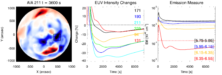
To demonstrate the capability of the model for reproducing the solar coronal dimming, we synthesize the EUV emissions of 6 AIA wavebands for two hours after the CME onset in the 2011 February 15 event (Schrijver et al., 2011; Jin et al., 2016). In addition, we calculate the Emission Measure (EM) in 4 temperature bins (). In Figure 1, we show the core dimming (near the source region) evolution in the simulation. The left panel in Figure 1 shows a base-difference image (by substracting the pre-event intensity) in AIA 211 Å at = 1 hour. The black box shows the sub-region where the EUV intensities and EMs are derived. In the middle panel of Figure 1, the EUV intensity evolution (represented by relative changes in percentage comparing with the pre-event values) in 2 hours for all 6 AIA wavebands is shown. We can see that the intensities in all 6 wavebands drop, which suggests the plasma depletion included by the CME. This is also evident in the EM calculation (right panel of Figure 1). By fitting the intensity curves, we can estimate the dimming recovery time is about 9 to 16 hours.
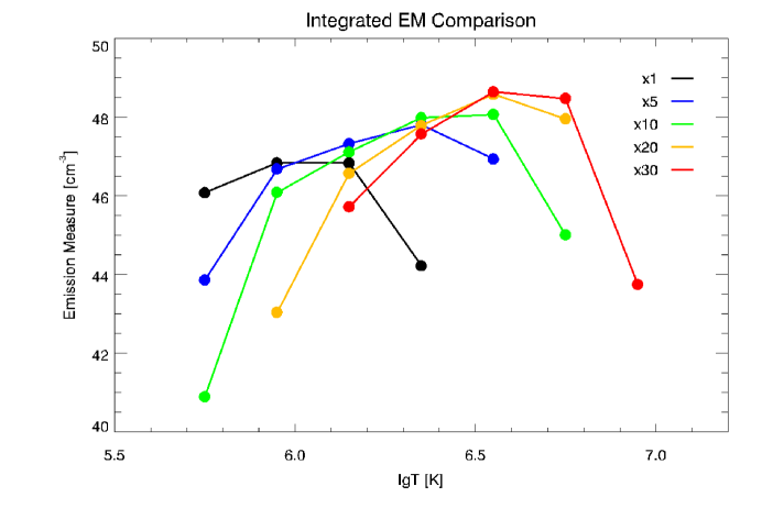
With higher mean surface magnetic flux density on the M dwarf or young Sun-like stars, their coronas are believed to be hotter than the solar case. By varying the in the model by 5, 10, 20, 30 times, we demonstrate this effect quantitatively in Figure 2. With the increasing magnetic field strength, the peak EM temperature shifts from 1 MK for the solar case to 5 MK for the stellar case with magnetic field 30 times stronger. Note that the peak EM temperature for the solar case is consistent with the dominant dimming lines in the solar observation (i.e., 171 Å and 193 Å, with emission temperatures around 1 MK). Therefore, even without simulating the CMEs, the steady-state corona solution is useful to estimate the dominant coronal dimming lines in the stellar cases with different magnetic flux densities.
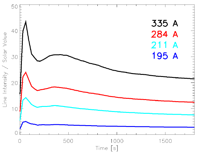
We then initiate CMEs with varying initial energies and into different steady-state coronal conditions. The simulation is switched to time-accurate mode to capture the CME eruption, and the MHD equations are solved in conservative form to guarantee the energy conservation during the eruption process. Here, we show two representative cases: one confined eruption and one explosive eruption. The confined eruption is due to the strong overlaying global coronal magnetic field that prevents the CME to escape (Alvarado-Gómez et al., 2018). In this case, since there is no plasma depletion involved, the EUV lines show no dimming features. Instead, due to the redistribution of the magnetic energy in the corona, it leads to a second peak in some EUV intensity profiles as shown in Figure 3. The second peak is more evident in the lines with higher emission temperature (e.g., 335 Å and 284 Å), which suggests the coronal plasma is dominant in these temperatures. This phenomenon is also frequently observed on the Sun and referred as EUV late-phase (e.g., Woods et al. 2011).
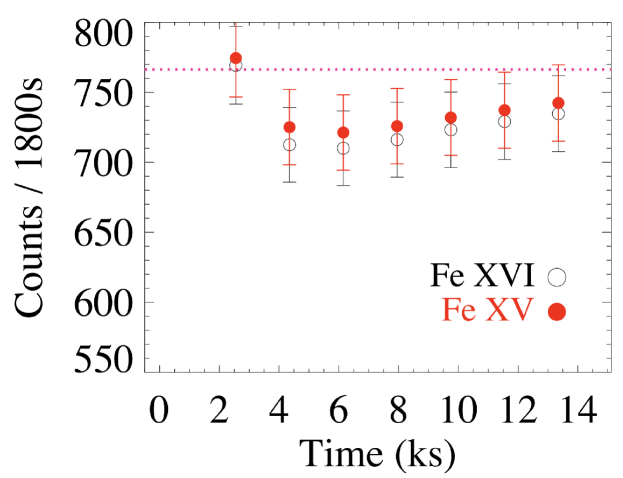
The second case is an explosive eruption in which the coronal mass is released into the interstellar space and leads to EUV coronal dimmings. In this case, the input is 5 times higher than the solar case. And the initial CME flux rope energy is about 1033 ergs. The resulting CME speed is 3000 km s-1, which is only slightly higher than the fast solar CMEs due to the stronger coronal field confinement. We simulate the coronal dynamical evolution for 4 hours after the CME eruption and synthesize the EUV line emissions. To further investigate the detectability of the dimming signals, we apply the instrument performance estimates from the Extreme-ultraviolet Stellar Characterization for Atmospheric Physics and Evolution (ESCAPE) mission concept, which provides extreme- and far-ultraviolet spectroscopy (70 - 1800 Å) to characterize the high energy radiation environment in the habitable zones around nearby stars (France et al., 2019). The EUV detector of the ESCAPE mission will be 100 times more sensitive than the previous EUVE mission (Craig et al., 1997). Figure 4 shows the simulated Fe XV 284 Å and Fe XVI 335 Å line emissions by assuming the star at 6 pc and using 30 minutes exposure time. The ISM absorption effect has been taken into account assuming (H I) = cm-2 (France et al., 2018). This preliminary result suggests that with better instrumentation, the stellar coronal dimmings associated with CMEs can be observed.
We summarize the main results as follows:
-
•
The coronal dimmings encode important information about CME energetics, CME-driven shock properties, and magnetic configuration of erupting flux ropes.
-
•
With higher magnetic flux density, the stellar dimming occurs in the higher temperature range than the solar case. With better instrumentation, the coronal dimming could be detected from the distant stars.
-
•
Our results show a proof-of-concept that the MHD model can be used for quantitative studies of CME-dimming relationships and applied to stellar cases. To get useful CME information from the future stellar observations, more detailed modeling studies are needed.
Christoffer KaroffHow would this look if you looked in the optical and not the UV?
Meng JinBecause the mass loss of the CME is mainly from the corona, the coronal dimming is not seen in the optical bands that dominate by photospheric emissions.
Acknowledgements.
M.Jin was supported by NASA’s SDO/AIA contract (NNG04EA00C) to LMSAL. We are thankful for the use of the NASA Supercomputer Pleiades at Ames and its helpful staff for making it possible to perform the simulations presented in this study. SDO is the first mission of NASA’s Living With a Star (LWS) Program.References
- Alvarado-Gómez et al. (2018) Alvarado-Gómez, J. D., Drake, J. J., Cohen, O., et al. 2018, ApJ, 862, 93
- Attrill et al. (2010) Attrill, G. D. R., Harra, L. K., van Driel-Gesztelyi, L., & Wills-Davey, M. J. 2010, Sol. Phys., 264, 119
- Aschwanden et al. (2009) Aschwanden, M. J., Nitta, N. V., Wuelser, J.-P., et al. 2009, ApJ, 706, 376
- Cheng & Qiu (2016) Cheng, J. X., & Qiu, J. 2016, ApJ, 825, 37
- Cohen et al. (2009) Cohen, O., Attrill, G. D. R., Manchester, W. B., IV, & Wills-Davey, M. J. 2009, ApJ, 705, 587-602
- Craig et al. (1997) Craig, N., Abbott, M., Finley, D., et al. 1997, ApJS, 113, 131
- Delaboudinière et al. (1995) Delaboudinière, J.-P., Artzner, G. E., Brunaud, J., et al. 1995, Sol. Phys., 162, 291
- Dissauer et al. (2018a) Dissauer, K., Veronig, A. M., Temmer, M., et al. 2018, ApJ, 855, 137
- Dissauer et al. (2018b) Dissauer, K., Veronig, A. M., Temmer, M., et al. 2018, ApJ, 863, 169
- Downs et al. (2012) Downs, C., Roussev, I. I., van der Holst, B., Lugaz, N., & Sokolov, I. V. 2012, ApJ, 750, 134
- Downs et al. (2015) Downs, C., Török, T., Titov, V., et al. 2015, AAS/AGU Triennial Earth-Sun Summit, 1, 304.01
- Gibson & Low (1998) Gibson, S. E., & Low, B. C. 1998, ApJ, 493, 460
- Hansen et al. (1974) Hansen, R. T., Garcia, C. J., Hansen, S. F., & Yasukawa, E. 1974, PASP, 86, 500
- Harra & Sterling (2001) Harra, L. K., & Sterling, A. C. 2001, ApJ, 561, L215
- Harra et al. (2007) Harra, L. K., Hara, H., Imada, S., et al. 2007, PASJ, 59, S801
- Harra et al. (2016) Harra, L. K., Schrijver, C. J., Janvier, M., et al. 2016, Sol. Phys., 291, 1761
- Harrison et al. (2003) Harrison, R. A., Bryans, P., Simnett, G. M., & Lyons, M. 2003, A&A, 400, 1071
- Hudson et al. (1996) Hudson, H. S., Acton, L. W., & Freeland, S. L. 1996, ApJ, 470, 629
- Imada et al. (2007) Imada, S., Hara, H., Watanabe, T., et al. 2007, PASJ, 59, S793
- Jin et al. (2009) Jin, M., Ding, M. D., Chen, P. F., Fang, C., & Imada, S. 2009, ApJ, 702, 27
- Jin et al. (2016) Jin, M., Schrijver, C. J., Cheung, M. C. M., et al. 2016, ApJ, 820, 16
- Jin et al. (2017a) Jin, M., Manchester, W. B., van der Holst, B., et al. 2017a, ApJ, 834, 172
- Jin et al. (2017b) Jin, M., Manchester, W. B., van der Holst, B., et al. 2017b, ApJ, 834, 173
- France et al. (2018) France, K., Arulanantham, N., Fossati, L., et al. 2018, ApJS, 239, 16
- France et al. (2019) France, K., Fleming, B. T., Drake, J. J., et al. 2019, Proc. SPIE 11118, UV, X-Ray, and Gamma-Ray Space Instrumentation for Astronomy XXI, 1111808
- Krista & Reinard (2013) Krista, L. D., & Reinard, A. 2013, ApJ, 762, 91
- Krista & Reinard (2017) Krista, L. D., & Reinard, A. A. 2017, ApJ, 839, 50
- Lemen et al. (2012) Lemen, J. R., Title, A. M., Akin, D. J., et al. 2012, Sol. Phys., 275, 17
- Lugaz et al. (2005) Lugaz, N., Manchester, IV, W. B., & Gombosi, T. I. 2005, ApJ, 634, 651
- Manchester et al. (2004a) Manchester, W. B., Gombosi, T. I., Roussev, I., de Zeeuw, D. L., Sokolov, I. V., Powell, K. G., Tóth, G., & Opher, M. 2004a, Journal of Geophysical Research (Space Physics), 109, 1102
- Manchester et al. (2004b) Manchester, W. B., Gombosi, T. I., Roussev, I., Ridley, A., de Zeeuw, D. L., Sokolov, I. V., Powell, K. G., & Tóth, G. 2004b, Journal of Geophysical Research (Space Physics), 109, 2107
- Manchester et al. (2014) Manchester, IV, W. B., van der Holst, B., & Lavraud, B. 2014, Plasma Physics and Controlled Fusion, 56, 064006
- Mason et al. (2014) Mason, J. P., Woods, T. N., Caspi, A., Thompson, B. J., & Hock, R. A. 2014, ApJ, 789, 61
- Mason et al. (2016) Mason, J. P., Woods, T. N., Webb, D. F., et al. 2016, ApJ, 830, 20
- Oran et al. (2013) Oran, R., van der Holst, B., Landi, E., et al. 2013, ApJ, 778, 176
- Oran et al. (2015) Oran, R., Landi, E., van der Holst, B., et al. 2015, ApJ, 806, 55
- Pesnell et al. (2012) Pesnell, W. D., Thompson, B. J., & Chamberlin, P. C. 2012, Sol. Phys., 275, 3
- Reinard & Biesecker (2008) Reinard, A. A., & Biesecker, D. A. 2008, ApJ, 674, 576-585
- Rust & Hildner (1976) Rust, D. M., & Hildner, E. 1976, Sol. Phys., 48, 381
- Schrijver et al. (2011) Schrijver, C. J., Aulanier, G., Title, A. M., Pariat, E., & Delannée, C. 2011, ApJ, 738, 167
- Sokolov et al. (2013) Sokolov, I. V., van der Holst, B., Oran, R., et al. 2013, ApJ, 764, 23
- Sterling & Hudson (1997) Sterling, A. C., & Hudson, H. S. 1997, ApJ, 491, L55
- Sterling et al. (2000) Sterling, A. C., Hudson, H. S., Thompson, B. J., & Zarro, D. M. 2000, ApJ, 532, 628
- Tian et al. (2012) Tian, H., McIntosh, S. W., Xia, L., He, J., & Wang, X. 2012, ApJ, 748, 106
- Thompson et al. (1998) Thompson, B. J., Plunkett, S. P., Gurman, J. B., et al. 1998, Geophys. Res. Lett., 25, 2465
- Thompson et al. (1999) Thompson, B. J., Gurman, J. B., Neupert, W. M., et al. 1999, ApJ, 517, L151
- Thompson et al. (2000) Thompson, B. J., Cliver, E. W., Nitta, N., Delannée, C., & Delaboudinière, J.-P. 2000, Geophys. Res. Lett., 27, 1431
- Tóth et al. (2012) Tóth, G., et al. 2012, Journal of Computational Physics, 231, 870
- van der Holst et al. (2014) van der Holst, B., Sokolov, I. V., Meng, X., et al. 2014, ApJ, 782, 81
- Woods et al. (2011) Woods, T. N., Hock, R., Eparvier, F., et al. 2011, ApJ, 739, 59
- Woods et al. (2012) Woods, T. N., Eparvier, F. G., Hock, R., et al. 2012, Sol. Phys., 275, 115
- Zarro et al. (1999) Zarro, D. M., Sterling, A. C., Thompson, B. J., Hudson, H. S., & Nitta, N. 1999, ApJ, 520, L139
- Zhukov & Auchère (2004) Zhukov, A. N., & Auchère, F. 2004, A&A, 427, 705