\eMail

[1]a.papapantoleon@tudelft.nl \eMail[2]p.yanez@outlook.de

\myThanks

[s]We thank Thibaut Lux for fruitful discussions during the work on these topics. AP gratefully acknowledges the financial support from the Hellenic Foundation for Research and Innovation Grant No. HFRI-FM17-2152.

Detection of arbitrage opportunities in multi-asset
derivatives markets

Antonis Papapantoleon    Paulo Yanez Sarmiento Delft Institute of Applied Mathematics, TU Delft, 2628 Delft, The Netherlands Institute of Applied and Computational Mathematics, FORTH, 70013 Heraklion, Greece Institute of Mathematics, TU Berlin, Straße des 17. Juni 136, 10623 Berlin, Germany
Abstract

We are interested in the existence of equivalent martingale measures and the detection of arbitrage opportunities in markets where several multi-asset derivatives are traded simultaneously. More specifically, we consider a financial market with multiple traded assets whose marginal risk-neutral distributions are known, and assume that several derivatives written on these assets are traded simultaneously. In this setting, there is a bijection between the existence of an equivalent martingale measure and the existence of a copula that couples these marginals. Using this bijection and recent results on improved Fréchet–Hoeffding bounds in the presence of additional information on functionals of a copula by Lux and Papapantoleon [18], we can extend the results of Tavin [33] on the detection of arbitrage opportunities to the general multi-dimensional case. More specifically, we derive sufficient conditions for the absence of arbitrage and formulate an optimization problem for the detection of a possible arbitrage opportunity. This problem can be solved efficiently using numerical optimization routines. The most interesting practical outcome is the following: we can construct a financial market where each multi-asset derivative is traded within its own no-arbitrage interval, and yet when considered together an arbitrage opportunity may arise.

\keyWords

Arbitrage, equivalent martingale measures, detection of arbitrage opportunities, multiple assets, multi-asset derivatives, copulas, improved Fréchet–Hoeffding bounds.

\keyAMSClassification

91G20, 62H05, 60E15. \keyJELClassification

1 Introduction

We consider a financial market where multiple assets and several derivatives written on single or multiple assets are traded simultaneously. Assuming we are given a set of traded prices for these multi-asset derivatives, we are interested in whether there exists an arbitrage-free model that is consistent with these prices or not. A consistent arbitrage-free model will exist if we can find an equivalent martingale measure such that we can describe these prices as discounted expected payoffs under this measure. We assume that the marginal risk-neutral distributions of the assets are known, e.g. they have been estimated from single-asset options prices using Breeden and Litzenberger [4]. Then, there exists a bijection between the existence of an equivalent martingale measure and the existence of a copula that couples these marginal distributions. Using recent results about improved Fréchet–Hoeffding bounds on copulas in the presence of additional information, we can formulate a sufficient condition for the existence of a copula and thus for the absence of arbitrage in this financial market. Moreover, the formulation of this condition as an optimization problem allows for the detection of an arbitrage opportunity via numerical optimization routines.

Arbitrage is a fundamental concept in economics and finance, because the modern theory of option valuation is rooted on the assumption of the absence of arbitrage, while it is also closely related with notions of equilibrium in financial markets. Arbitrage is also a concept of practical importance, as financial institutions are interested in ensuring that their systems for option valuation, simulation, scenario generation, etc, are free of arbitrage, in order to be useful and relevant. Therefore, topics related to the existence of arbitrage and the consistency of arbitrage-free models with given traded prices are of significant theoretical and practical interest.

There is a sufficiently rich literature by now devoted to the case where a single asset and options on this asset are traded in a financial market. Laurent and Leisen [17] in their pioneering work provide a procedure to check for the absence of arbitrage in a discrete set of market data. Carr and Madan [7] provide a sufficient condition for the absence of arbitrage in a market where countably-infinite many European options with discrete strikes can be traded. These results where later generalized and extended by Cousot [8], by Buehler [5], and in particular by Davis and Hobson [10] who provided necessary and sufficient conditions for the existence of an arbitrage-free model consistent with a set of market prices. More recently, Gerhold and Gülüm [14] considered the same problem in case the only observables are the bid and ask prices of the underlying asset.

The literature is not that developed when one turns to multiple underlying assets and multi-asset derivatives. Actually, to the best of our knowledge, the only work treating this problem until very recently was Tavin [33]. The setting here is exactly the same as in Tavin [33], i.e. the author considers multiple underlying assets with known risk-neutral marginals and several traded derivatives on multiple assets, and provides two methods for detecting arbitrage opportunities, one based on Bernstein copulas and another based on improved Fréchet–Hoeffding bounds, which is however restricted to the two-asset case. In our work, we extend the results of Tavin [33] to the general multi-asset case using the recent results of Lux and Papapantoleon [18] on improved Fréchet–Hoeffding bounds for d𝑑d-copulas in the presence of additional information on functionals of a copula, with d2𝑑2d\geq 2.

In a very recent work, Neufeld et al. [22] developed numerical methods for the computation of model-free bounds for multi-asset option prices in the presence of other traded multi-asset derivatives. Their results are supported by a Fundamental Theorem of Asset Pricing for their setting, and the numerical methods are used for the detection of arbitrage opportunities as well. Compared to that work, our method is conceptually and computationally simpler, while both methods are numerically efficient. However, our method only yields the existence of an arbitrage opportunity, while the method of Neufeld et al. [22] also delivers the portfolio that generates the arbitrage. Moreover, the two settings are not the same; here we assume that the marginals are known, while in Neufeld et al. [22] the authors assume the existence of finitely many traded European options for each single asset. Therefore, the two methods are not directly comparable.

Let us also mention that there exist several articles on the computation of model-free bounds for multi-asset option prices; see e.g. Dhaene et al. [11, 12], Hobson et al. [15, 16], d’Aspremont and El Ghaoui [9], Peña et al. [23], Tankov [32] and Lux and Papapantoleon [18] to mention a fraction of this literature, while we refer the reader to [18] and [22] for more comprehensive literature reviews. These methods could also be used, in principle, to detect arbitrage opportunities, although this has not been pursued yet.

The remainder of this article is structured as follows: In Section 2 we review some necessary results about copulas, quasi-copulas and improved Fréchet–Hoeffding bounds. In Section 3 we present results on integration and stochastic dominance for quasi-copulas; these include also a new representation of the integral with respect to a quasi-copula that could be of independent interest. In Section 4 we revisit the bijection between the existence of an equivalent martingale measure and a copula that couples the marginals of the underlying assets already present in Tavin [33], and derive necessary conditions for the absence of arbitrage in the presence of several multi-asset derivatives traded simultaneously. In Section 5 we apply our results in models with three underlying assets. In particular, we show that we can construct a financial market where each multi-asset derivative is traded within its own no-arbitrage interval, and yet when considered together an arbitrage opportunity may arise. Finally, the appendix collects some additional results.

2 Copulas, quasi-copulas and improved Fréchet–Hoeffding bounds

This section serves as an introduction to the notation that will be used throughout this work, as well as to the basic notion of copulas, quasi-copulas and (improved) Fréchet–Hoeffding bounds. Let d2𝑑2d\geq 2 be an integer, and set 𝕀=[0,1]𝕀01\mathbb{I}=[0,1] and 𝟏=(1,,1)d111superscript𝑑\mathbf{1}=(1,\dots,1)\in\mathbb{R}^{d}. In the sequel, boldface letters, such as 𝐮𝐮\mathbf{u} or 𝐯𝐯\mathbf{v}, denote vectors in 𝕀dsuperscript𝕀𝑑\mathbb{I}^{d} or dsuperscript𝑑\mathbb{R}^{d} with entries u1,,udsubscript𝑢1subscript𝑢𝑑u_{1},\dots,u_{d} or v1,,vdsubscript𝑣1subscript𝑣𝑑v_{1},\dots,v_{d}, while we distinguish strictly between \subset and \subseteq, i.e. if JI𝐽𝐼J\subset I then JI𝐽𝐼J\neq I. Moreover, for a univariate distribution function F𝐹F we define its inverse as F1(u):=inf{x|F(x)u}assignsuperscript𝐹1𝑢infimumconditional-set𝑥𝐹𝑥𝑢F^{-1}(u):=\inf\{x\in\mathbb{R}\,|\,F(x)\geq u\}, while we call a function f:d:𝑓superscript𝑑f:\mathbb{R}^{d}\rightarrow\mathbb{R} left-continuous if it is left-continuous in each component.

Definition 2.1.

A function Q:𝕀d𝕀:𝑄superscript𝕀𝑑𝕀Q:\mathbb{I}^{d}\rightarrow\mathbb{I} is a d𝑑d-quasi-copula if it satisfies the following properties:

  • (C1)

    boundary condition: Q(u1,,ui=0,,ud)=0Q(u_{1},\dots,u_{i}=0,\dots,u_{d})=0, for all 1id1𝑖𝑑1\leq i\leq d.

  • (C2)

    uniform marginals: Q(1,,1,ui,1,,1)=ui𝑄11subscript𝑢𝑖11subscript𝑢𝑖Q(1,\dots,1,u_{i},1,\dots,1)=u_{i}, for all 1id1𝑖𝑑1\leq i\leq d.

  • (C3)

    Q𝑄Q is non-decreasing in each component.

  • (C4)

    Q𝑄Q is Lipschitz continuous, i.e. for all 𝐮,𝐯𝕀d𝐮𝐯superscript𝕀𝑑\mathbf{u},\mathbf{v}\in\mathbb{I}^{d}

    |Q(𝐮)Q(𝐯)|i=1d|uivi|.𝑄𝐮𝑄𝐯superscriptsubscript𝑖1𝑑subscript𝑢𝑖subscript𝑣𝑖\displaystyle|Q(\mathbf{u})-Q(\mathbf{v})|\leq\sum_{i=1}^{d}|u_{i}-v_{i}|\,.

Moreover, Q𝑄Q is a d𝑑d-copula if it satisfies in addition:

  • (C5)

    Q𝑄Q is d𝑑d-increasing.

\blacklozenge

The set of all d𝑑d-quasi-copulas is denoted by 𝒬dsuperscript𝒬𝑑\mathcal{Q}^{d} and the set of all d𝑑d-copulas by 𝒞dsuperscript𝒞𝑑\mathcal{C}^{d}. Obviously, 𝒞d𝒬dsuperscript𝒞𝑑superscript𝒬𝑑\mathcal{C}^{d}\subset\mathcal{Q}^{d}. Moreover, we call Q𝒬d𝒞d𝑄superscript𝒬𝑑superscript𝒞𝑑Q\in\mathcal{Q}^{d}\setminus\mathcal{C}^{d} a proper quasi-copula. In case the dimension d𝑑d is clear, we refer to a d𝑑d-(quasi-)copula as a (quasi-)copula.

There exists a clear link between copulas and probability distributions. In fact, for C𝒞d𝐶superscript𝒞𝑑C\in\mathcal{C}^{d} and univariate distribution functions F1,,Fdsubscript𝐹1subscript𝐹𝑑F_{1},\dots,F_{d},

F(𝐱):=C(F1(x1),,Fd(xd))assign𝐹𝐱𝐶subscript𝐹1subscript𝑥1subscript𝐹𝑑subscript𝑥𝑑\displaystyle F(\mathbf{x}):=C\big{(}F_{1}(x_{1}),\dots,F_{d}(x_{d})\big{)} (2.1)

defines a d𝑑d-dimensional distribution function with marginals F1,,Fdsubscript𝐹1subscript𝐹𝑑F_{1},\dots,F_{d}. The celebrated theorem of Sklar [31] tells us that the converse is also true, i.e. given a d𝑑d-dimensional distribution function F𝐹F with univariate marginals F1,,Fdsubscript𝐹1subscript𝐹𝑑F_{1},\dots,F_{d}, there exists a copula C𝐶C such that (2.1) holds true. We will call C𝐶C the copula corresponding to F𝐹F.

Let Q𝒬d𝑄superscript𝒬𝑑Q\in\mathcal{Q}^{d}. We define its survival function Q^:𝕀d𝕀:^𝑄superscript𝕀𝑑𝕀\widehat{Q}:\mathbb{I}^{d}\rightarrow\mathbb{I} as follows:

Q^(𝐮):=VQ(×i=1d(ui,1]),assign^𝑄𝐮subscript𝑉𝑄superscriptsubscript𝑖1𝑑subscript𝑢𝑖1\displaystyle\widehat{Q}(\mathbf{u}):=V_{Q}\Big{(}\mathop{\raisebox{-2.15277pt}{\hbox{\huge{$\times$}}}}_{i=1}^{d}(u_{i},1]\Big{)}, (2.2)

and denote by 𝒞^d:={C^|C𝒞d\widehat{\mathcal{C}}^{d}:=\{\widehat{C}\,|\,C\in\mathcal{C}^{d}}. A well-known result states that if C𝒞d𝐶superscript𝒞𝑑C\in\mathcal{C}^{d}, then 𝐮C^(𝟏𝐮)maps-to𝐮^𝐶1𝐮\mathbf{u}\mapsto\widehat{C}(\mathbf{1}-\mathbf{u}) is again a copula, namely the survival copula of C𝐶C, while there exists also a version of Sklar’s theorem for survival copulas. In case Q𝑄Q is a proper quasi-copula, then 𝐮Q^(𝟏𝐮)maps-to𝐮^𝑄1𝐮\mathbf{u}\mapsto\widehat{Q}(\mathbf{1}-\mathbf{u}) is not a quasi-copula in general; see e.g. Example 2.5 in Lux and Papapantoleon [18].

Let us now define a partial order on 𝒬dsuperscript𝒬𝑑\mathcal{Q}^{d}, and thus also on 𝒞dsuperscript𝒞𝑑\mathcal{C}^{d}.

Definition 2.2.

Let Q1,Q2𝒬dsubscript𝑄1subscript𝑄2superscript𝒬𝑑Q_{1},Q_{2}\in\mathcal{Q}^{d}.

  • (i)

    If Q1(𝐮)Q2(𝐮)subscript𝑄1𝐮subscript𝑄2𝐮Q_{1}(\mathbf{u})\leq Q_{2}(\mathbf{u}) for all 𝐮𝕀d𝐮superscript𝕀𝑑\mathbf{u}\in\mathbb{I}^{d}, then Q1subscript𝑄1Q_{1} is smaller than Q2subscript𝑄2Q_{2} in the lower orthant order, denoted by Q1LOQ2subscriptprecedes-or-equals𝐿𝑂subscript𝑄1subscript𝑄2Q_{1}\preceq_{LO}Q_{2}.

  • (ii)

    If Q^1(𝐮)Q^2(𝐮)subscript^𝑄1𝐮subscript^𝑄2𝐮\widehat{Q}_{1}(\mathbf{u})\leq\widehat{Q}_{2}(\mathbf{u}) for all 𝐮𝕀d𝐮superscript𝕀𝑑\mathbf{u}\in\mathbb{I}^{d}, then Q1subscript𝑄1Q_{1} is smaller than Q2subscript𝑄2Q_{2} in the upper orthant order, denoted by Q1UOQ2subscriptprecedes-or-equals𝑈𝑂subscript𝑄1subscript𝑄2Q_{1}\preceq_{UO}Q_{2}.

\blacklozenge

The celebrated Fréchet–Hoeffding bounds provide upper and lower bounds for all quasi-copulas with respect to the lower orthant order. Indeed, for Q𝒬d𝑄superscript𝒬𝑑Q\in\mathcal{Q}^{d}, we have that

Wd(𝐮):=max{i=1duid+1,0}Q(𝐮)min{u1,,ud}=:Md(𝐮),\displaystyle W_{d}(\mathbf{u}):=\max\bigg{\{}\sum_{i=1}^{d}u_{i}-d+1,0\bigg{\}}\leq Q(\mathbf{u})\leq\min\{u_{1},\dots,u_{d}\}=:M_{d}(\mathbf{u}),

for all 𝐮𝕀d𝐮superscript𝕀𝑑\mathbf{u}\in\mathbb{I}^{d}, which readily implies that WdLOCLOMdsubscriptprecedes-or-equals𝐿𝑂subscript𝑊𝑑𝐶subscriptprecedes-or-equals𝐿𝑂subscript𝑀𝑑W_{d}\preceq_{LO}C\preceq_{LO}M_{d}. Wdsubscript𝑊𝑑W_{d} and Mdsubscript𝑀𝑑M_{d} are respectively called the lower and upper Fréchet–Hoeffding bounds. Analogous results hold true for the upper orthant order and the survival functions, i.e. we have that

Wd(𝟏𝐮)C^(𝐮)Md(𝟏𝐮), for all 𝐮𝕀d,formulae-sequencesubscript𝑊𝑑1𝐮^𝐶𝐮subscript𝑀𝑑1𝐮 for all 𝐮superscript𝕀𝑑\displaystyle W_{d}(\mathbf{1}-\mathbf{u})\leq\widehat{C}(\mathbf{u})\leq M_{d}(\mathbf{1}-\mathbf{u}),\quad\text{ for all }\mathbf{u}\in\mathbb{I}^{d}\,,\

while an easy computation shows that Md(𝟏)=M^d()M_{d}(\mathbf{1}-\cdot)=\widehat{M}_{d}(\cdot) for all d2𝑑2d\geq 2, while Wd(𝟏)=W^d()W_{d}(\mathbf{1}-\cdot)=\widehat{W}_{d}(\cdot) only for d=2𝑑2d=2.

The Fréchet–Hoeffding bounds are derived under the assumption that the marginal distributions are fully known and the copula is fully unknown. However, in several applications such as finance and insurance, partial information on the copula is available from market data. Therefore, there has been intensive research in the last decade on improving the Fréchet–Hoeffding bounds by adding partial information on the copula, see e.g. Nelsen [21], Tankov [32], Puccetti et al. [24], Lux and Papapantoleon [18, 19]; see also Rüschendorf [29] and reference therein. Earlier results in this direction, using the language of optimal transport, appear in Rachev and Rüschendorf [25]. The following results from Lux and Papapantoleon [18, Sec. 3] describe improved Fréchet–Hoeffding bounds under the assumption that the copula is known in a subset of its domain, or that a functional of the copula is known. Analogous statements for survival copulas appear in [18, Appendix A].

Let 𝒮[0,1]d𝒮superscript01𝑑\mathcal{S}\subseteq[0,1]^{d} be compact and Q𝒬dsuperscript𝑄superscript𝒬𝑑Q^{*}\in\mathcal{Q}^{d}. Define the set

𝒬𝒮,Q:={Q𝒬d|Q(𝐱)=Q(𝐱)for all𝐱𝒮}.assignsuperscript𝒬𝒮superscript𝑄conditional-set𝑄superscript𝒬𝑑𝑄𝐱superscript𝑄𝐱for all𝐱𝒮\displaystyle\mathcal{Q}^{\mathcal{S},Q^{*}}:=\big{\{}Q\in\mathcal{Q}^{d}\,|\,Q(\mathbf{x})=Q^{*}(\mathbf{x})\,\,\textit{for all}\,\,\mathbf{x}\in\mathcal{S}\big{\}}\,.

Then, for all Q𝒬𝒮,Q𝑄superscript𝒬𝒮superscript𝑄Q\in\mathcal{Q}^{\mathcal{S},Q^{*}}

QL𝒮,QLOQLOQU𝒮,Q,subscriptprecedes-or-equals𝐿𝑂superscriptsubscript𝑄𝐿𝒮superscript𝑄𝑄subscriptprecedes-or-equals𝐿𝑂superscriptsubscript𝑄𝑈𝒮superscript𝑄\displaystyle Q_{L}^{\mathcal{S},Q^{*}}\preceq_{LO}Q\preceq_{LO}Q_{U}^{\mathcal{S},Q^{*}}\,,

where the improved Fréchet–Hoeffding bounds QL𝒮,Q,QU𝒮,Q𝒬dsuperscriptsubscript𝑄𝐿𝒮superscript𝑄superscriptsubscript𝑄𝑈𝒮superscript𝑄superscript𝒬𝑑Q_{L}^{\mathcal{S},Q^{*}},Q_{U}^{\mathcal{S},Q^{*}}\in\mathcal{Q}^{d} and are provided by

QL𝒮,Q(𝐮)superscriptsubscript𝑄𝐿𝒮superscript𝑄𝐮\displaystyle Q_{L}^{\mathcal{S},Q^{*}}(\mathbf{u}) =max{0,i=1duid+1,max𝐱𝒮{Q(𝐱)i=1d(xiui)+}},absent0superscriptsubscript𝑖1𝑑subscript𝑢𝑖𝑑1subscript𝐱𝒮superscript𝑄𝐱superscriptsubscript𝑖1𝑑superscriptsubscript𝑥𝑖subscript𝑢𝑖\displaystyle=\max\Big{\{}0,\sum_{i=1}^{d}u_{i}-d+1,\max_{\mathbf{x}\in\mathcal{S}}\big{\{}Q^{*}(\mathbf{x})-\sum_{i=1}^{d}(x_{i}-u_{i})^{+}\big{\}}\Big{\}},
QU𝒮,Q(𝐮)superscriptsubscript𝑄𝑈𝒮superscript𝑄𝐮\displaystyle Q_{U}^{\mathcal{S},Q^{*}}(\mathbf{u}) =min{u1,,ud,min𝐱𝒮{Q(𝐱)+i=1d(uixi)+}}.absentsubscript𝑢1subscript𝑢𝑑subscript𝐱𝒮superscript𝑄𝐱superscriptsubscript𝑖1𝑑superscriptsubscript𝑢𝑖subscript𝑥𝑖\displaystyle=\min\Big{\{}u_{1},\dots,u_{d},\min_{\mathbf{x}\in\mathcal{S}}\big{\{}Q^{*}(\mathbf{x})+\sum_{i=1}^{d}(u_{i}-x_{i})^{+}\big{\}}\Big{\}}\,.
Remark 2.3.

A natural question is whether the bounds QL𝒮,Qsuperscriptsubscript𝑄𝐿𝒮superscript𝑄Q_{L}^{\mathcal{S},Q^{*}} and QU𝒮,Qsuperscriptsubscript𝑄𝑈𝒮superscript𝑄Q_{U}^{\mathcal{S},Q^{*}} are copulas or proper quasi-copulas. Nelsen [21] showed that in the case of 𝒮𝒮\mathcal{S} being a singleton and for d=2𝑑2d=2 the lower and upper improved Fréchet-Hoeffding bounds are copulas using the concept of shuffles of M2subscript𝑀2M_{2}. This statement was generalized by Tankov [32] and Bernard et al. [2], still for d=2𝑑2d=2, under certain “monotonicity” conditions. On the contrary, Lux and Papapantoleon [18] showed that for d>2𝑑2d>2, the improved Fréchet–Hoeffding bounds are copulas only in trivial cases and proper quasi-copulas otherwise. Moreover, Bartl et al. [1] showed that the improved Fréchet–Hoeffding bounds are not pointwise sharp (or best-possible), even in d=2𝑑2d=2, if the aforementioned “monotonicity” conditions are violated. \blacklozenge

The next result provides improved Fréchet–Hoeffding bounds in case the value of a functional of the copula is known. Examples of functionals could be the correlation or another measure of dependence (e.g. Kendall’s τ𝜏\tau or Spearman’s ρ𝜌\rho), but also prices of multi-asset options in a mathematical finance context. Let ρ:𝒬d:𝜌superscript𝒬𝑑\rho:\mathcal{Q}^{d}\rightarrow\mathbb{R} be non-decreasing with respect to the lower orthant order and continuous with respect to the pointwise convergence of quasi-copulas, and consider the set of quasi-copulas

𝒬ρ,θ:={Q𝒬d|ρ(Q)=θ},assignsuperscript𝒬𝜌𝜃conditional-set𝑄superscript𝒬𝑑𝜌𝑄𝜃\displaystyle\mathcal{Q}^{\rho,\theta}:=\big{\{}Q\in\mathcal{Q}^{d}\,|\,\rho(Q)=\theta\big{\}}\,, (2.3)

for θ[ρ(Wd),ρ(Md)]𝜃𝜌subscript𝑊𝑑𝜌subscript𝑀𝑑\theta\in[\rho(W_{d}),\rho(M_{d})]. Then, for all Q𝒬ρ,θ𝑄superscript𝒬𝜌𝜃Q\in\mathcal{Q}^{\rho,\theta}, holds

QLρ,θLOQLOQUρ,θ,subscriptprecedes-or-equals𝐿𝑂superscriptsubscript𝑄𝐿𝜌𝜃𝑄subscriptprecedes-or-equals𝐿𝑂superscriptsubscript𝑄𝑈𝜌𝜃\displaystyle Q_{L}^{\rho,\theta}\preceq_{LO}Q\preceq_{LO}Q_{U}^{\rho,\theta}\,,

where the improved Fréchet–Hoeffding bounds QLρ,θ,QUρ,θ𝒬dsuperscriptsubscript𝑄𝐿𝜌𝜃superscriptsubscript𝑄𝑈𝜌𝜃superscript𝒬𝑑Q_{L}^{\rho,\theta},Q_{U}^{\rho,\theta}\in\mathcal{Q}^{d} are provided by

QLρ,θ(𝐮):=assignsuperscriptsubscript𝑄𝐿𝜌𝜃𝐮absent\displaystyle Q_{L}^{\rho,\theta}(\mathbf{u}):= {ρ+1(𝐮,θ),ifθ[ρ+(𝐮,Wd(𝐮)),ρ(Md)],Wd(𝐮),otherwise,casessubscriptsuperscript𝜌1𝐮𝜃if𝜃subscript𝜌𝐮subscript𝑊𝑑𝐮𝜌subscript𝑀𝑑otherwisesubscript𝑊𝑑𝐮otherwiseotherwise\displaystyle\begin{cases}\rho^{-1}_{+}(\mathbf{u},\theta)\,,\quad\textit{if}\,\,\theta\in[\rho_{+}(\mathbf{u},W_{d}(\mathbf{u})),\rho(M_{d})],\\ W_{d}(\mathbf{u})\,,\quad\quad\textit{otherwise}\,,\end{cases} (2.4)
QUρ,θ(𝐮):=assignsuperscriptsubscript𝑄𝑈𝜌𝜃𝐮absent\displaystyle Q_{U}^{\rho,\theta}(\mathbf{u}):= {ρ1(𝐮,θ),ifθ[ρ(Wd),ρ(𝐮,Md(𝐮))],Md(𝐮),otherwise.casessubscriptsuperscript𝜌1𝐮𝜃if𝜃𝜌subscript𝑊𝑑subscript𝜌𝐮subscript𝑀𝑑𝐮otherwisesubscript𝑀𝑑𝐮otherwiseotherwise\displaystyle\begin{cases}\rho^{-1}_{-}(\mathbf{u},\theta)\,,\quad\textit{if}\,\,\theta\in[\rho(W_{d}),\rho_{-}(\mathbf{u},M_{d}(\mathbf{u}))],\\ M_{d}(\mathbf{u})\,,\quad\quad\textit{otherwise}.\end{cases} (2.5)

The improved Fréchet–Hoeffding bounds QLρ,θsuperscriptsubscript𝑄𝐿𝜌𝜃Q_{L}^{\rho,\theta} and QUρ,θsuperscriptsubscript𝑄𝑈𝜌𝜃Q_{U}^{\rho,\theta} are actually the infimum and supremum over the set 𝒬ρ,θsuperscript𝒬𝜌𝜃\mathcal{Q}^{\rho,\theta}. Here we use the following notation: for 𝐮[0,1]d𝐮superscript01𝑑\mathbf{u}\in[0,1]^{d}, let rI𝐮=[Wd(𝐮),Md(𝐮)]𝑟subscript𝐼𝐮subscript𝑊𝑑𝐮subscript𝑀𝑑𝐮r\in I_{\mathbf{u}}=[W_{d}(\mathbf{u}),M_{d}(\mathbf{u})] and Q𝒬dsuperscript𝑄superscript𝒬𝑑Q^{*}\in\mathcal{Q}^{d} with Q(𝐮)=rsuperscript𝑄𝐮𝑟Q^{*}(\mathbf{u})=r, and define QL{𝐮},r:=QL{𝐮},Q,QU{𝐮},r:=QU{𝐮},Qformulae-sequenceassignsuperscriptsubscript𝑄𝐿𝐮𝑟superscriptsubscript𝑄𝐿𝐮superscript𝑄assignsuperscriptsubscript𝑄𝑈𝐮𝑟superscriptsubscript𝑄𝑈𝐮superscript𝑄Q_{L}^{\{\mathbf{u}\},r}:=Q_{L}^{\{\mathbf{u}\},Q^{*}},Q_{U}^{\{\mathbf{u}\},r}:=Q_{U}^{\{\mathbf{u}\},Q^{*}} and

ρ(𝐮,r):=ρ(QL{𝐮},r) and ρ+(𝐮,r):=ρ(QU{𝐮},r).formulae-sequenceassignsubscript𝜌𝐮𝑟𝜌superscriptsubscript𝑄𝐿𝐮𝑟 and assignsubscript𝜌𝐮𝑟𝜌superscriptsubscript𝑄𝑈𝐮𝑟\displaystyle\rho_{-}(\mathbf{u},r):=\rho\big{(}Q_{L}^{\{\mathbf{u}\},r}\big{)}\quad\text{ and }\quad\rho_{+}(\mathbf{u},r):=\rho\big{(}Q_{U}^{\{\mathbf{u}\},r}\big{)}\,.

Then, for fixed 𝐮𝐮\mathbf{u}, the maps rρ(𝐮,r)maps-to𝑟subscript𝜌𝐮𝑟r\mapsto\rho_{-}(\mathbf{u},r) and rρ+(𝐮,r)maps-to𝑟subscript𝜌𝐮𝑟r\mapsto\rho_{+}(\mathbf{u},r) are non-decreasing and continuous. Hence, we can define their inverse mappings

θρ1(𝐮,θ)maps-to𝜃superscriptsubscript𝜌1𝐮𝜃\displaystyle\theta\mapsto\rho_{-}^{-1}(\mathbf{u},\theta) :=max{rI𝐮:ρ(𝐮,r)=θ},assignabsent:𝑟subscript𝐼𝐮subscript𝜌𝐮𝑟𝜃\displaystyle:=\max\{r\in I_{\mathbf{u}}:\rho_{-}(\mathbf{u},r)=\theta\},
θρ+1(𝐮,θ)maps-to𝜃superscriptsubscript𝜌1𝐮𝜃\displaystyle\theta\mapsto\rho_{+}^{-1}(\mathbf{u},\theta) :=min{rI𝐮:ρ+(𝐮,r)=θ},assignabsent:𝑟subscript𝐼𝐮subscript𝜌𝐮𝑟𝜃\displaystyle:=\min\{r\in I_{\mathbf{u}}:\rho_{+}(\mathbf{u},r)=\theta\},

for all θ𝜃\theta such that the sets are non-empty. Analogous statements for non-increasing functionals are relegated to Appendix A.

3 Integration and stochastic dominance for quasi-copulas

This section provides results on the definition of integrals with respect to quasi-copulas and on stochastic dominance for quasi-copulas. These results are largely taken from Lux and Papapantoleon [18, Sec. 5], however we also provide a new representation of the integral with respect to a quasi-copula, as well as some useful results on stochastic dominance for quasi-copulas. Stochastic dominance results for copulas were introduced in Rüschendorf [27], see also the book of Müller and Stoyan [20], while analogous results for quasi-copulas in the 2-dimensional case appear in Tankov [32]. A special case of the results on stochastic dominance presented below appears already in Rüschendorf [28].

Let (Ω,,)Ω(\Omega,\mathcal{F},\mathbb{P}) be a probability space. Consider an +dsubscriptsuperscript𝑑\mathbb{R}^{d}_{+}-valued random vector 𝐗=(X1,,Xd)𝐗subscript𝑋1subscript𝑋𝑑\mathbf{X}=(X_{1},\dots,X_{d}) with distribution function F𝐹F and marginals F1,,Fdsubscript𝐹1subscript𝐹𝑑F_{1},\dots,F_{d}. Then, from Sklar’s Theorem, we know there exists a copula C𝒞d𝐶superscript𝒞𝑑C\in\mathcal{C}^{d} such that

(X1<x1,,Xd<xd)=C(F1(x1),,Fd(xd))formulae-sequencesubscript𝑋1subscript𝑥1subscript𝑋𝑑subscript𝑥𝑑𝐶subscript𝐹1subscript𝑥1subscript𝐹𝑑subscript𝑥𝑑\displaystyle\mathbb{P}(X_{1}<x_{1},\dots,X_{d}<x_{d})=C\big{(}F_{1}(x_{1}),\dots,F_{d}(x_{d})\big{)}

and

(X1>x1,,Xd>xd)=C^(F1(x1),,Fd(xd)).formulae-sequencesubscript𝑋1subscript𝑥1subscript𝑋𝑑subscript𝑥𝑑^𝐶subscript𝐹1subscript𝑥1subscript𝐹𝑑subscript𝑥𝑑\displaystyle\mathbb{P}(X_{1}>x_{1},\dots,X_{d}>x_{d})=\widehat{C}\big{(}F_{1}(x_{1}),\dots,F_{d}(x_{d})\big{)}\,.

Hence, there exists an induced measure dC(F1(x1),,F(xd))d𝐶subscript𝐹1subscript𝑥1𝐹subscript𝑥𝑑\mathrm{d}C\big{(}F_{1}(x_{1}),\dots,F(x_{d})\big{)} on +dsubscriptsuperscript𝑑\mathbb{R}^{d}_{+}. Consider a function f:+d:𝑓subscriptsuperscript𝑑f:\mathbb{R}^{d}_{+}\rightarrow\mathbb{R}. In this section we focus on calculating 𝔼[f(𝐗)]𝔼delimited-[]𝑓𝐗\mathbb{E}[f(\mathbf{X})] and its properties with respect to C𝐶C. Assuming the marginals are given, we define the expectation operator πfsubscript𝜋𝑓\pi_{f} as follows

πf(C):=𝔼[f(𝐗)]assignsubscript𝜋𝑓𝐶𝔼delimited-[]𝑓𝐗\displaystyle\pi_{f}(C):=\mathbb{E}[f(\mathbf{X})] =+df(x1,,xd)dC(F1(x1),,Fd(xd))absentsubscriptsubscriptsuperscript𝑑𝑓subscript𝑥1subscript𝑥𝑑differential-d𝐶subscript𝐹1subscript𝑥1subscript𝐹𝑑subscript𝑥𝑑\displaystyle=\int\limits_{\mathbb{R}^{d}_{+}}f(x_{1},\dots,x_{d})\,\mathrm{d}C\big{(}F_{1}(x_{1}),\dots,F_{d}(x_{d})\big{)} (3.1)
=[0,1]df(F11(u1),,Fd1(ud))dC(u1,,ud).absentsubscriptsuperscript01𝑑𝑓subscriptsuperscript𝐹11subscript𝑢1subscriptsuperscript𝐹1𝑑subscript𝑢𝑑differential-d𝐶subscript𝑢1subscript𝑢𝑑\displaystyle=\int\limits_{[0,1]^{d}}f\big{(}F^{-1}_{1}(u_{1}),\dots,F^{-1}_{d}(u_{d})\big{)}\,\mathrm{d}C(u_{1},\dots,u_{d})\,.

However, if Q𝑄Q is a proper quasi-copula then dQ(F1(x1),,F(xd))d𝑄subscript𝐹1subscript𝑥1𝐹subscript𝑥𝑑\mathrm{d}Q\big{(}F_{1}(x_{1}),\dots,F(x_{d})\big{)} does not induce a measure anymore, because the Q𝑄Q-volume VQsubscript𝑉𝑄V_{Q} is not necessarily positive. The idea is now to switch the function we integrate against, i.e. to perform a Fubini transformation. In order to do so, the function f𝑓f has to induce a measure. Therefore, we consider functions of the following type.

Definition 3.1.
  1. (i)

    A function f:+d:𝑓subscriptsuperscript𝑑f:\mathbb{R}^{d}_{+}\rightarrow\mathbb{R} is called ΔΔ\Delta-antitonic if for every subset I={i1,,in}{1,,d}𝐼subscript𝑖1subscript𝑖𝑛1𝑑I=\{i_{1},\dots,i_{n}\}\subseteq\{1,\dots,d\} with |I|1𝐼1|I|\geq 1 and every hypercube ×j=1n(aj,bj]+nsuperscriptsubscript𝑗1𝑛subscript𝑎𝑗subscript𝑏𝑗subscriptsuperscript𝑛\mathop{\raisebox{-2.15277pt}{\hbox{\huge{$\times$}}}}_{j=1}^{n}(a_{j},b_{j}]\subset\mathbb{R}^{n}_{+}

    (1)nΔa1,b1i1Δan,bninf0.superscript1𝑛superscriptsubscriptΔsubscript𝑎1subscript𝑏1subscript𝑖1superscriptsubscriptΔsubscript𝑎𝑛subscript𝑏𝑛subscript𝑖𝑛𝑓0\displaystyle(-1)^{n}\Delta_{a_{1},b_{1}}^{i_{1}}\circ\dots\circ\Delta_{a_{n},b_{n}}^{i_{n}}f\geq 0\,.
  2. (ii)

    A function f:+d:𝑓subscriptsuperscript𝑑f:\mathbb{R}^{d}_{+}\rightarrow\mathbb{R} is called ΔΔ\Delta-monotonic if for every subset I={i1,,in}{1,,d}𝐼subscript𝑖1subscript𝑖𝑛1𝑑I=\{i_{1},\dots,i_{n}\}\subseteq\{1,\dots,d\} with |I|1𝐼1|I|\geq 1 and every hypercube ×j=1n(aj,bj]+nsuperscriptsubscript𝑗1𝑛subscript𝑎𝑗subscript𝑏𝑗subscriptsuperscript𝑛\mathop{\raisebox{-2.15277pt}{\hbox{\huge{$\times$}}}}_{j=1}^{n}(a_{j},b_{j}]\subset\mathbb{R}^{n}_{+}

    Δa1,b1i1Δan,bninf0.superscriptsubscriptΔsubscript𝑎1subscript𝑏1subscript𝑖1superscriptsubscriptΔsubscript𝑎𝑛subscript𝑏𝑛subscript𝑖𝑛𝑓0\displaystyle\Delta_{a_{1},b_{1}}^{i_{1}}\circ\dots\circ\Delta_{a_{n},b_{n}}^{i_{n}}f\geq 0\,.

\blacklozenge

We will frequently deal with marginals of functions f𝑓f and quasi-copulas Q𝑄Q, therefore the following definition is useful.

Definition 3.2.
  1. (i)

    Let f:+d:𝑓subscriptsuperscript𝑑f:\mathbb{R}^{d}_{+}\rightarrow\mathbb{R}. Then, for I={i1,,in}{1,,d}𝐼subscript𝑖1subscript𝑖𝑛1𝑑I=\{i_{1},\dots,i_{n}\}\subseteq\{1,\dots,d\}, we define the I𝐼I-margin of f𝑓f as

    fI:+n,(xi1,,xin)f(x1,,xd),with xk=0 for kI.:subscript𝑓𝐼formulae-sequencesubscriptsuperscript𝑛formulae-sequencemaps-tosubscript𝑥subscript𝑖1subscript𝑥subscript𝑖𝑛𝑓subscript𝑥1subscript𝑥𝑑with subscript𝑥𝑘0 for 𝑘𝐼\displaystyle f_{I}:\mathbb{R}^{n}_{+}\rightarrow\mathbb{R}\,,(x_{i_{1}},\dots,x_{i_{n}})\mapsto f(x_{1},\dots,x_{d}),\text{with }x_{k}=0\text{ for }k\notin I\,.
  2. (ii)

    Let Q𝒬d𝑄superscript𝒬𝑑Q\in\mathcal{Q}^{d}. Then, for I={i1,,in}{1,,d}𝐼subscript𝑖1subscript𝑖𝑛1𝑑I=\{i_{1},\dots,i_{n}\}\subseteq\{1,\dots,d\}, we define the I𝐼I-margin of Q𝑄Q as

    QI:[0,1]n[0,1],(ui1,,uin)Q(u1,,ud),with uk=1 for kI.:subscript𝑄𝐼formulae-sequencesuperscript01𝑛01formulae-sequencemaps-tosubscript𝑢subscript𝑖1subscript𝑢subscript𝑖𝑛𝑄subscript𝑢1subscript𝑢𝑑with subscript𝑢𝑘1 for 𝑘𝐼\displaystyle Q_{I}:[0,1]^{n}\rightarrow[0,1]\,,(u_{i_{1}},\dots,u_{i_{n}})\mapsto Q(u_{1},\dots,u_{d}),\text{with }u_{k}=1\text{ for }k\notin I\,.

\blacklozenge

According to well-known results, we can associate a measure to every left-continuous and ΔΔ\Delta-monotonic or ΔΔ\Delta-antitonic function f:+d:𝑓subscriptsuperscript𝑑f:\mathbb{R}^{d}_{+}\rightarrow\mathbb{R} via

μfI():=0 and μfI(R):=VfI(R),formulae-sequenceassignsubscript𝜇subscript𝑓𝐼0 and assignsubscript𝜇subscript𝑓𝐼𝑅subscript𝑉subscript𝑓𝐼𝑅\displaystyle\mu_{f_{I}}(\emptyset):=0\ \ \text{ and }\ \ \mu_{f_{I}}\big{(}R\big{)}:=V_{f_{I}}\big{(}R\big{)}\,, (3.2)

for every hyperrectangle R|I|𝑅superscript𝐼R\subseteq\mathbb{R}^{|I|}. Then, we get that μfIsubscript𝜇subscript𝑓𝐼\mu_{f_{I}} is a positive measure on +|I|subscriptsuperscript𝐼\mathbb{R}^{|I|}_{+} if f𝑓f is ΔΔ\Delta-monotonic, and that (1)nμfIsuperscript1𝑛subscript𝜇subscript𝑓𝐼(-1)^{n}\mu_{f_{I}} is a positive measure on +|I|subscriptsuperscript𝐼\mathbb{R}^{|I|}_{+} if f𝑓f is ΔΔ\Delta-antitonic. If I={1,,d}𝐼1𝑑I=\{1,\dots,d\}, then we write μfsubscript𝜇𝑓\mu_{f} instead of μfIsubscript𝜇subscript𝑓𝐼\mu_{f_{I}}. In addition, we define μf:=δ0assignsubscript𝜇subscript𝑓subscript𝛿0\mu_{f_{\emptyset}}:=\delta_{0}, where δ𝛿\delta denotes the Dirac measure.

Remark 3.3.
\thlabel

minusf Let f:+d:𝑓subscriptsuperscript𝑑f:\mathbb{R}^{d}_{+}\rightarrow\mathbb{R} be a left-continuous function, such that f𝑓-f is either ΔΔ\Delta-antitonic or ΔΔ\Delta-monotonic. Then, we have for I={i1,,in}{1,,d}𝐼subscript𝑖1subscript𝑖𝑛1𝑑I=\{i_{1},\dots,i_{n}\}\subseteq\{1,\dots,d\} with |I|1𝐼1|I|\geq 1 and every hypercube ×j=1n(aj,bj]+nsuperscriptsubscript𝑗1𝑛subscript𝑎𝑗subscript𝑏𝑗subscriptsuperscript𝑛\mathop{\raisebox{-2.15277pt}{\hbox{\huge{$\times$}}}}_{j=1}^{n}(a_{j},b_{j}]\subset\mathbb{R}^{n}_{+} that

(1)nΔa1,b1i1Δan,bninfsuperscript1𝑛superscriptsubscriptΔsubscript𝑎1subscript𝑏1subscript𝑖1superscriptsubscriptΔsubscript𝑎𝑛subscript𝑏𝑛subscript𝑖𝑛𝑓\displaystyle(-1)^{n}\Delta_{a_{1},b_{1}}^{i_{1}}\circ\dots\circ\Delta_{a_{n},b_{n}}^{i_{n}}f 0,if f is Δ-antitonic, andabsent0if f is Δ-antitonic, and\displaystyle\leq 0\,,\quad\textit{if $\,-f$ is $\Delta$-antitonic, and}
Δa1,b1i1Δan,bninfsuperscriptsubscriptΔsubscript𝑎1subscript𝑏1subscript𝑖1superscriptsubscriptΔsubscript𝑎𝑛subscript𝑏𝑛subscript𝑖𝑛𝑓\displaystyle\Delta_{a_{1},b_{1}}^{i_{1}}\circ\dots\circ\Delta_{a_{n},b_{n}}^{i_{n}}f 0,if f is Δ-monotonic.absent0if f is Δ-monotonic.\displaystyle\leq 0\,,\quad\textit{if $\,-f$ is $\Delta$-monotonic.}

Hence, μfIsubscript𝜇subscript𝑓𝐼-\mu_{f_{I}} is a positive measure on +|I|subscriptsuperscript𝐼\mathbb{R}^{|I|}_{+} if f𝑓-f is ΔΔ\Delta-monotonic and (1)n+1μfIsuperscript1𝑛1subscript𝜇subscript𝑓𝐼(-1)^{n+1}\mu_{f_{I}} is a positive measure on +|I|subscriptsuperscript𝐼\mathbb{R}^{|I|}_{+} if f𝑓-f is ΔΔ\Delta-antitonic. \blacklozenge

The following definitions show how the measure induced by the I𝐼I-marginals of functions in conjunction with the I𝐼I-marginals of copulas, can be used to define an integration operation. We define iteratively:

for |I|=0:φfI(C):=:for 𝐼0assignsuperscriptsubscript𝜑𝑓𝐼𝐶absent\displaystyle\textrm{for }|I|=0:\varphi_{f}^{I}(C):= f(0,,0),𝑓00\displaystyle f(0,\dots,0)\,, (3.3)
for |I|=1:φfI(C):=:for 𝐼1assignsuperscriptsubscript𝜑𝑓𝐼𝐶absent\displaystyle\textrm{for }|I|=1:\varphi_{f}^{I}(C):= +fi1(xi1)dFi1(xi1),subscriptsubscriptsubscript𝑓subscript𝑖1subscript𝑥subscript𝑖1differential-dsubscript𝐹subscript𝑖1subscript𝑥subscript𝑖1\displaystyle\int\limits_{\mathbb{R}_{+}}f_{i_{1}}(x_{i_{1}})\,\mathrm{d}F_{i_{1}}(x_{i_{1}})\,,
for |I|=n2:φfI(C):=:for 𝐼𝑛2assignsuperscriptsubscript𝜑𝑓𝐼𝐶absent\displaystyle\textrm{for }|I|=n\geq 2:\varphi_{f}^{I}(C):= +|I|C^I(Fi1(xi1),,Fin(xin))dμfI(xi1,,xin)subscriptsubscriptsuperscript𝐼subscript^𝐶𝐼subscript𝐹subscript𝑖1subscript𝑥subscript𝑖1subscript𝐹subscript𝑖𝑛subscript𝑥subscript𝑖𝑛differential-dsubscript𝜇subscript𝑓𝐼subscript𝑥subscript𝑖1subscript𝑥subscript𝑖𝑛\displaystyle\int\limits_{\mathbb{R}^{|I|}_{+}}\widehat{C}_{I}\big{(}F_{i_{1}}(x_{i_{1}}),\dots,F_{i_{n}}(x_{i_{n}})\big{)}\,\mathrm{d}\mu_{f_{I}}(x_{i_{1}},\dots,x_{i_{n}})
+JI(1)n+1|J|φfJ(C),subscript𝐽𝐼superscript1𝑛1𝐽superscriptsubscript𝜑𝑓𝐽𝐶\displaystyle+\sum_{J\subset I}(-1)^{n+1-|J|}\varphi_{f}^{J}(C)\,,

where C^Isubscript^𝐶𝐼\widehat{C}_{I} denotes the survival function of the I𝐼I-margin of C𝐶C. Lux and Papapantoleon [18, Prop. 5.3] proved that the operator φf{1,,d}(C)superscriptsubscript𝜑𝑓1𝑑𝐶\varphi_{f}^{\{1,\dots,d\}}(C) defined above coincides with the expectation operator πf(C)subscript𝜋𝑓𝐶\pi_{f}(C) in (3.1) in case f:d:𝑓superscript𝑑f:\mathbb{R}^{d}\rightarrow\mathbb{R} is left-continuous, ΔΔ\Delta-antitonic or ΔΔ\Delta-monotonic and C𝒞d𝐶superscript𝒞𝑑C\in\mathcal{C}^{d}. However, the operator φf{1,,d}(C)superscriptsubscript𝜑𝑓1𝑑𝐶\varphi_{f}^{\{1,\dots,d\}}(C) does not depend on C𝐶C being a copula, and can be also defined for quasi-copulas. This motivates the following definition, which generalizes the expectation operator to quasi-copulas.

Definition 3.4.

Let f:d:𝑓superscript𝑑f:\mathbb{R}^{d}\rightarrow\mathbb{R} be left-continuous, ΔΔ\Delta-antitonic or ΔΔ\Delta-monotonic and d2𝑑2d\geq 2. Then, the expectation operator is defined as follows πf:𝒬d,Qπf(Q):subscript𝜋𝑓formulae-sequencesuperscript𝒬𝑑maps-to𝑄subscript𝜋𝑓𝑄\pi_{f}:\mathcal{Q}^{d}\rightarrow\mathbb{R},\,Q\mapsto\pi_{f}(Q) , with

πf(Q):=φf{1,,d}(Q).assignsubscript𝜋𝑓𝑄superscriptsubscript𝜑𝑓1𝑑𝑄\displaystyle\pi_{f}(Q):=\varphi_{f}^{\{1,\dots,d\}}(Q)\,.

\blacklozenge

Remark 3.5.

Let Q𝒬d𝑄superscript𝒬𝑑Q\in\mathcal{Q}^{d} and consider its survival function Q^^𝑄\widehat{Q}. We define the dual to the operations φfIsuperscriptsubscript𝜑𝑓𝐼\varphi_{f}^{I} and πfsubscript𝜋𝑓\pi_{f} as follows:

φ^fI(Q^):=φfI(Q) and π^f(Q^):=πf(Q),formulae-sequenceassignsuperscriptsubscript^𝜑𝑓𝐼^𝑄superscriptsubscript𝜑𝑓𝐼𝑄 and assignsubscript^𝜋𝑓^𝑄subscript𝜋𝑓𝑄\displaystyle\widehat{\varphi}_{f}^{I}\big{(}\widehat{Q}\big{)}:=\varphi_{f}^{I}\big{(}Q\big{)}\quad\text{ and }\quad\widehat{\pi}_{f}\big{(}\widehat{Q}\big{)}:=\pi_{f}\big{(}Q\big{)}\,,

since both operations actually only depend on the knowledge of Q^^𝑄\widehat{Q} and not of Q𝑄Q itself. \blacklozenge

Remark 3.6.

Using that Vfi((0,x])=fi(x)fi(0)subscript𝑉subscript𝑓𝑖0𝑥subscript𝑓𝑖𝑥subscript𝑓𝑖0V_{f_{i}}\big{(}(0,x]\big{)}=f_{i}(x)-f_{i}(0), we can rewrite the case |I|={i}𝐼𝑖|I|=\{i\} from (3.3) as follows

+fi(xi)dFi(xi)=+(1Fi(xi))dμfi(xi)+fi(0).subscriptsubscriptsubscript𝑓𝑖subscript𝑥𝑖differential-dsubscript𝐹𝑖subscript𝑥𝑖subscriptsubscript1subscript𝐹𝑖subscript𝑥𝑖differential-dsubscript𝜇subscript𝑓𝑖subscript𝑥𝑖subscript𝑓𝑖0\displaystyle\int\limits_{\mathbb{R}_{+}}f_{i}(x_{i})\,\mathrm{d}F_{i}(x_{i})=\int\limits_{\mathbb{R}_{+}}\big{(}1-F_{i}(x_{i})\big{)}\mathrm{d}\mu_{f_{i}}(x_{i})+f_{i}(0)\,. (3.4)

Depending on the way the integrals are computed, this representation might be more useful. If we compute the one-dimensional integrals as in (3.3) instead of (3.4), then we do not need f{i}subscript𝑓𝑖f_{\{i\}} to induce a measure. Therefore, in [18] the authors define ΔΔ\Delta-antitonic and ΔΔ\Delta-monotonic in the sense that only fI,|I|2subscript𝑓𝐼𝐼2f_{I},|I|\geq 2, has to induce a measure. \blacklozenge

The following result provides an alternative, simpler representation for the expectation operator πf(Q)subscript𝜋𝑓𝑄\pi_{f}(Q).

Theorem 3.7.
\thlabel

lemmaPhi Let f:d:𝑓superscript𝑑f:\mathbb{R}^{d}\rightarrow\mathbb{R} be left-continuous, ΔΔ\Delta-antitonic or ΔΔ\Delta-monotonic and Q𝒬d𝑄superscript𝒬𝑑Q\in\mathcal{Q}^{d}. Then, the following representation holds

πf(Q)subscript𝜋𝑓𝑄\displaystyle\pi_{f}(Q) =+dQ^(F1(x1),,Fd(xd))dμf(x1,,xd)absentsubscriptsubscriptsuperscript𝑑^𝑄subscript𝐹1subscript𝑥1subscript𝐹𝑑subscript𝑥𝑑differential-dsubscript𝜇𝑓subscript𝑥1subscript𝑥𝑑\displaystyle=\int\limits_{\mathbb{R}^{d}_{+}}\widehat{Q}\big{(}F_{1}(x_{1}),\dots,F_{d}(x_{d})\big{)}\,\mathrm{d}\mu_{f}(x_{1},\dots,x_{d})
+JI|J|=d1+d1Q^J(F1(xi1),,Fid1(xid1))dμfJ(xi1,,xid1)subscript𝐽𝐼𝐽𝑑1subscriptsubscriptsuperscript𝑑1subscript^𝑄𝐽subscript𝐹1subscript𝑥subscript𝑖1subscript𝐹subscript𝑖𝑑1subscript𝑥subscript𝑖𝑑1differential-dsubscript𝜇subscript𝑓𝐽subscript𝑥subscript𝑖1subscript𝑥subscript𝑖𝑑1\displaystyle\quad+\sum_{\begin{subarray}{c}J\subset I\\ |J|=d-1\end{subarray}}\,\,\,\int\limits_{\mathbb{R}^{d-1}_{+}}\widehat{Q}_{J}\big{(}F_{1}(x_{i_{1}}),\dots,F_{i_{d-1}}(x_{i_{d-1}})\big{)}\,\mathrm{d}\mu_{f_{J}}(x_{i_{1}},\dots,x_{i_{d-1}})
++i=1d+f{i}(xi)dFi(xi)(d1)f(0,,0)superscriptsubscript𝑖1𝑑subscriptsubscriptsubscript𝑓𝑖subscript𝑥𝑖differential-dsubscript𝐹𝑖subscript𝑥𝑖𝑑1𝑓00\displaystyle\quad+\dots+\sum_{i=1}^{d}\,\,\int\limits_{\mathbb{R}_{+}}f_{\{i\}}(x_{i})\,\mathrm{d}F_{i}(x_{i})-(d-1)f(0,\dots,0)
=f(0,,0)+n=1dJIJ={i1,,in}+nQ^J(F1(xi1),,Fin(xin))dμfJ(xi1,,xin).absent𝑓00superscriptsubscript𝑛1𝑑subscript𝐽𝐼𝐽subscript𝑖1subscript𝑖𝑛subscriptsubscriptsuperscript𝑛subscript^𝑄𝐽subscript𝐹1subscript𝑥subscript𝑖1subscript𝐹subscript𝑖𝑛subscript𝑥subscript𝑖𝑛differential-dsubscript𝜇subscript𝑓𝐽subscript𝑥subscript𝑖1subscript𝑥subscript𝑖𝑛\displaystyle=f(0,\dots,0)+\sum_{n=1}^{d}\,\sum_{\begin{subarray}{c}J\subseteq I\\ J=\{i_{1},\dots,i_{n}\}\end{subarray}}\,\int\limits_{\mathbb{R}^{n}_{+}}\widehat{Q}_{J}\big{(}F_{1}(x_{i_{1}}),\dots,F_{i_{n}}(x_{i_{n}})\big{)}\,\mathrm{d}\mu_{f_{J}}(x_{i_{1}},\dots,x_{i_{n}})\,. (3.5)

\blacklozenge

Proof 3.8.

Without loss of generality we assume I={1,,d}𝐼1𝑑I=\{1,\dots,d\}. For |I|=1𝐼1|I|=1 the claim is given by (3.4). Now assume it holds all n<d𝑛𝑑n<d for some d𝑑d\in\mathbb{N}. Define

αJ:=assignsubscript𝛼𝐽absent\displaystyle\alpha_{J}:= +|J|Q^J(F1(xi1),,Fin(xin))dμfJ(xi1,,xin),|J|1,subscriptsubscriptsuperscript𝐽subscript^𝑄𝐽subscript𝐹1subscript𝑥subscript𝑖1subscript𝐹subscript𝑖𝑛subscript𝑥subscript𝑖𝑛differential-dsubscript𝜇subscript𝑓𝐽subscript𝑥subscript𝑖1subscript𝑥subscript𝑖𝑛𝐽1\displaystyle\int\limits_{\mathbb{R}^{|J|}_{+}}\widehat{Q}_{J}\big{(}F_{1}(x_{i_{1}}),\dots,F_{i_{n}}(x_{i_{n}})\big{)}\,\mathrm{d}\mu_{f_{J}}(x_{i_{1}},\dots,x_{i_{n}})\,,\,|J|\geq 1\,,
α:=assignsubscript𝛼absent\displaystyle\alpha_{\emptyset}:= f(0,,0).𝑓00\displaystyle f(0,\dots,0)\,.

Then we deduce by (3.3) and the induction hypothesis

φfI(Q)superscriptsubscript𝜑𝑓𝐼𝑄\displaystyle\varphi_{f}^{I}(Q) =αI+JI(1)d+1|J|φfJ(Q)absentsubscript𝛼𝐼subscript𝐽𝐼superscript1𝑑1𝐽superscriptsubscript𝜑𝑓𝐽𝑄\displaystyle=\alpha_{I}+\sum_{J\subset I}(-1)^{d+1-|J|}\varphi_{f}^{J}(Q)
=αI+JI(1)d+1|J|JJαJ.absentsubscript𝛼𝐼subscript𝐽𝐼superscript1𝑑1𝐽subscriptsuperscript𝐽𝐽subscript𝛼superscript𝐽\displaystyle=\alpha_{I}+\sum_{J\subset I}(-1)^{d+1-|J|}\sum_{J^{\prime}\subseteq J}\alpha_{J^{\prime}}\,. (3.6)

Hence, we have to show that for every JIsuperscript𝐽𝐼J^{\prime}\subset I the term αJsubscript𝛼superscript𝐽\alpha_{J^{\prime}} appears exactly once in (3.6) with positive sign. Consider J={j1,,jk}J={i1,,in}superscript𝐽subscript𝑗1subscript𝑗𝑘𝐽subscript𝑖1subscript𝑖𝑛J^{\prime}=\{j_{1},\dots,j_{k}\}\subseteq J=\{i_{1},\dots,i_{n}\}. There are (dknk)binomial𝑑𝑘𝑛𝑘\binom{d-k}{n-k} many JI𝐽𝐼J\subset I with JJsuperscript𝐽𝐽J^{\prime}\subseteq J because for J\J\𝐽superscript𝐽J\backslash J^{\prime} we can choose nk𝑛𝑘n-k elements out of I\J\𝐼superscript𝐽I\backslash J^{\prime}. We have

JI(1)d+1|J|JJαJsubscript𝐽𝐼superscript1𝑑1𝐽subscriptsuperscript𝐽𝐽subscript𝛼superscript𝐽\displaystyle\sum_{J\subset I}(-1)^{d+1-|J|}\sum_{J^{\prime}\subseteq J}\alpha_{J^{\prime}} =k=0|J|=knn=kd1(1)d+1n(dknk)αJ.absentsuperscriptsubscript𝑘0superscript𝐽𝑘𝑛superscriptsubscript𝑛𝑘𝑑1superscript1𝑑1𝑛binomial𝑑𝑘𝑛𝑘subscript𝛼superscript𝐽\displaystyle=\sum_{\begin{subarray}{c}k=0\\ |J^{\prime}|=k\end{subarray}}^{n}\sum_{n=k}^{d-1}(-1)^{d+1-n}\binom{d-k}{n-k}\alpha_{J^{\prime}}\,.

Further,

n=kd1(1)d+1n(dknk)={n=0dk1(1)n+1(dkn),if dk is even,n=0dk1(1)n(dkn),if dk is odd.superscriptsubscript𝑛𝑘𝑑1superscript1𝑑1𝑛binomial𝑑𝑘𝑛𝑘casessuperscriptsubscript𝑛0𝑑𝑘1superscript1𝑛1binomial𝑑𝑘𝑛if dk is even,superscriptsubscript𝑛0𝑑𝑘1superscript1𝑛binomial𝑑𝑘𝑛if dk is odd.\displaystyle\sum_{n=k}^{d-1}(-1)^{d+1-n}\binom{d-k}{n-k}=\begin{cases}\sum\limits_{n=0}^{d-k-1}(-1)^{n+1}\binom{d-k}{n},&\,\textrm{if $d-k$ is even,}\\ \sum\limits_{n=0}^{d-k-1}(-1)^{n}\binom{d-k}{n},&\,\textrm{if $d-k$ is odd.}\end{cases}

Since l=0m(1)l(ml)=0superscriptsubscript𝑙0𝑚superscript1𝑙binomial𝑚𝑙0\sum_{l=0}^{m}(-1)^{l}\binom{m}{l}=0, m𝑚m\in\mathbb{N}, we have n=kd1(1)d+1n(dknk)=1superscriptsubscript𝑛𝑘𝑑1superscript1𝑑1𝑛binomial𝑑𝑘𝑛𝑘1\sum_{n=k}^{d-1}(-1)^{d+1-n}\binom{d-k}{n-k}=1 for both cases. This proves (3.5). \blacklozenge

Now we can show that the expectation operator πfsubscript𝜋𝑓\pi_{f} is increasing or decreasing with respect to the lower and upper orthant order, depending on the properties of the function f𝑓f.

Proposition 3.9.

Let Q1,Q2𝒬dsubscript𝑄1subscript𝑄2superscript𝒬𝑑Q_{1},Q_{2}\in\mathcal{Q}^{d} and f:+d:𝑓superscriptsubscript𝑑f:\mathbb{R}_{+}^{d}\rightarrow\mathbb{R}. Then

  1. (i)

    for all f𝑓f ΔΔ\Delta-antitonic s.t. the integrals exist

    Q1LOQ2πf(Q1)πf(Q2),subscriptprecedes-or-equals𝐿𝑂subscript𝑄1subscript𝑄2subscript𝜋𝑓subscript𝑄1subscript𝜋𝑓subscript𝑄2\displaystyle Q_{1}\preceq_{LO}Q_{2}\Longrightarrow\pi_{f}(Q_{1})\leq\pi_{f}(Q_{2})\,,
  2. (ii)

    for all f𝑓f ΔΔ\Delta-monotonic s.t. the integrals exist

    Q1UOQ2πf(Q1)πf(Q2).subscriptprecedes-or-equals𝑈𝑂subscript𝑄1subscript𝑄2subscript𝜋𝑓subscript𝑄1subscript𝜋𝑓subscript𝑄2\displaystyle Q_{1}\preceq_{UO}Q_{2}\Longrightarrow\pi_{f}(Q_{1})\leq\pi_{f}(Q_{2})\,.
  3. (iii)

    for all f𝑓-f ΔΔ\Delta-antitonic s.t. the integrals exist

    Q1LOQ2πf(Q1)πf(Q2),subscriptprecedes-or-equals𝐿𝑂subscript𝑄1subscript𝑄2subscript𝜋𝑓subscript𝑄1subscript𝜋𝑓subscript𝑄2\displaystyle Q_{1}\preceq_{LO}Q_{2}\Longrightarrow\pi_{f}(Q_{1})\geq\pi_{f}(Q_{2})\,,
  4. (iv)

    for all f𝑓-f ΔΔ\Delta-monotonic s.t. the integrals exist

    Q1UOQ2πf(Q1)πf(Q2).subscriptprecedes-or-equals𝑈𝑂subscript𝑄1subscript𝑄2subscript𝜋𝑓subscript𝑄1subscript𝜋𝑓subscript𝑄2\displaystyle Q_{1}\preceq_{UO}Q_{2}\Longrightarrow\pi_{f}(Q_{1})\geq\pi_{f}(Q_{2})\,.

\blacklozenge

Proof 3.10.

The first two statements are Lux and Papapantoleon [18, Theorem 5.5], while the next two are a direct consequence of them and Remark LABEL:minusf. \blacklozenge

4 Copulas and arbitrage

In this section, we apply the results on improved Fréchet–Hoeffding bounds and on stochastic dominance for quasi-copulas to mathematical finance. We will first derive bounds for the arbitrage-free prices of certain classes of multi-asset derivatives. Then, we will formulate a necessary condition for the absence of arbitrage in markets where several multi-asset derivatives are traded simultaneously.

4.1 Model and assumptions

Let (Ω,,)Ω(\Omega,\mathcal{F},\mathbb{P}) be a probability space, where Ω=dΩsuperscript𝑑\Omega=\mathbb{R}^{d}. We consider the following financial market model: There exists one time period with initial time t=0𝑡0t=0 and final time t=T<𝑡𝑇t=T<\infty. Let d2𝑑2d\geq 2. There exist d+1𝑑1d+1 non-redundant primary assets denoted by B,S1,,Sd𝐵superscript𝑆1superscript𝑆𝑑B,S^{1},\dots,S^{d}. We assume that their initial prices are known, i.e. (B0,S01,,S0d)+d+1subscript𝐵0subscriptsuperscript𝑆10subscriptsuperscript𝑆𝑑0subscriptsuperscript𝑑1(B_{0},S^{1}_{0},\dots,S^{d}_{0})\in\mathbb{R}^{d+1}_{+}. B𝐵B denotes the risk-free asset that earns the interest rate r0𝑟0r\geq 0 and, for the sake of simplicity, we set BT=1subscript𝐵𝑇1B_{T}=1, while ST1,,STdsubscriptsuperscript𝑆1𝑇subscriptsuperscript𝑆𝑑𝑇S^{1}_{T},\dots,S^{d}_{T} are +subscript\mathbb{R}_{+}-valued random variables on the given probability space.

This framework contains discrete- and continuous-time models as well, however we are only interested in the distribution of the random vector ST1,,STdsubscriptsuperscript𝑆1𝑇subscriptsuperscript𝑆𝑑𝑇S^{1}_{T},\dots,S^{d}_{T}. This information is sufficient for the valuation of European vanilla derivatives, while the path dynamics are not necessary. In the examples presented in the following section, the random vector is modeled according to the Black and Scholes [3] model and an exponential Lévy model; cf. Eberlein [13]. The marginal distributions can be obtained by calibrating a parametric model to European option prices maturing at T𝑇T or by extracting the implied distributions from option prices using e.g. the Breeden and Litzenberger [4] formula.

A probability measure \mathbb{Q} on (Ω,)Ω(\Omega,\mathcal{F}), equivalent to \mathbb{P}, that satisfies

S0i=B0𝔼[STi],i=1,,d,formulae-sequencesubscriptsuperscript𝑆𝑖0subscript𝐵0subscript𝔼delimited-[]subscriptsuperscript𝑆𝑖𝑇𝑖1𝑑\displaystyle S^{i}_{0}=B_{0}\,\mathbb{E}_{\mathbb{Q}}\big{[}S^{i}_{T}\big{]},\quad i=1,\dots,d\,\,,

is called an equivalent martingale measure (EMM) for our financial market. The existence of an equivalent martingale measure and the absence of arbitrage have a well-known implication for the pricing of derivatives on STisubscriptsuperscript𝑆𝑖𝑇S^{i}_{T}. Consider a European derivative of STisubscriptsuperscript𝑆𝑖𝑇S^{i}_{T} with payoff H(STi)𝐻subscriptsuperscript𝑆𝑖𝑇H(S^{i}_{T}) at time T𝑇T, where H𝐻H is a function such that 𝔼[H(STi)]subscript𝔼delimited-[]𝐻subscriptsuperscript𝑆𝑖𝑇\mathbb{E}_{\mathbb{Q}}[H(S^{i}_{T})] exists. Then, the arbitrage-free price is provided by

H0i=B0𝔼[H(STi)],i=1,,d.formulae-sequencesuperscriptsubscript𝐻0𝑖subscript𝐵0subscript𝔼delimited-[]𝐻subscriptsuperscript𝑆𝑖𝑇𝑖1𝑑\displaystyle H_{0}^{i}=B_{0}\,\mathbb{E}_{\mathbb{Q}}\big{[}H(S^{i}_{T})\big{]},\quad i=1,\dots,d.

We assume that the risk-neutral marginal distributions of each STisuperscriptsubscript𝑆𝑇𝑖S_{T}^{i} are known and unique for all i=1,,d𝑖1𝑑i=1,\dots,d, i.e. the univariate marginal distribution of STisuperscriptsubscript𝑆𝑇𝑖S_{T}^{i} under \mathbb{Q} is equal for all EMMs \mathbb{Q}. We further assume that these distributions are continuous, and denote them by Fisubscript𝐹𝑖F_{i}, i.e.

(ST1+,,STi1+,STix,STi+1+,,STd+)=Fi(x),formulae-sequencesubscriptsuperscript𝑆1𝑇subscriptformulae-sequencesubscriptsuperscript𝑆𝑖1𝑇subscriptformulae-sequencesubscriptsuperscript𝑆𝑖𝑇𝑥formulae-sequencesubscriptsuperscript𝑆𝑖1𝑇subscriptsubscriptsuperscript𝑆𝑑𝑇subscriptsubscript𝐹𝑖𝑥\displaystyle\mathbb{Q}\big{(}S^{1}_{T}\in\mathbb{R}_{+},\dots,S^{i-1}_{T}\in\mathbb{R}_{+},S^{i}_{T}\leq x,S^{i+1}_{T}\in\mathbb{R}_{+},\dots,S^{d}_{T}\in\mathbb{R}_{+}\big{)}=F_{i}(x)\,, (4.1)

for all i=1,,d𝑖1𝑑i=1,\dots,d. Let 𝒫𝒫\mathscr{P} denote the set of all EMMs for our financial market model, i.e. 𝒫={|, MM,Ficontinuous and satisfies (4.1)}𝒫conditional-setsimilar-to MMsubscript𝐹𝑖continuous and satisfies (4.1)\mathscr{P}=\{\mathbb{Q}\,|\,\mathbb{Q}\sim\mathbb{P},\mathbb{Q}\text{ MM},F_{i}\ \text{continuous and satisfies \eqref{marginalsMartingaleMeasure}}\}. The assumption that the marginal distributions are known is not unrealistic, because their dynamics can be derived from market data; see e.g. Breeden and Litzenberger [4]. This property implies, by the second Fundamental Theorem of Asset Pricing, that the prices of single-asset options are unique, and is referred to in the literature as static-completeness of a financial market, see e.g. Carr and Madan [6]. Let us stress that this does not imply |𝒫|=1𝒫1|\mathscr{P}|=1, because the dependence structure of S1,,Sdsuperscript𝑆1superscript𝑆𝑑S^{1},\dots,S^{d} might not be uniquely determined.

The financial market, beside options on the single assets S1,,Sdsuperscript𝑆1superscript𝑆𝑑S^{1},\dots,S^{d}, consists also of a finite number of European multi-asset derivatives, denoted by Z1,,Zqsuperscript𝑍1superscript𝑍𝑞Z^{1},\dots,Z^{q}, for q𝑞q\in\mathbb{N}. Their final payoffs at time T𝑇T are given by

ZTi=zi(ST1,,STd),i=1,,q,formulae-sequencesubscriptsuperscript𝑍𝑖𝑇subscript𝑧𝑖subscriptsuperscript𝑆1𝑇subscriptsuperscript𝑆𝑑𝑇𝑖1𝑞\displaystyle Z^{i}_{T}=z_{i}\big{(}S^{1}_{T},\dots,S^{d}_{T}\big{)}\,,\quad i=1,\dots,q,

where the payoff functions zi:+d+:subscript𝑧𝑖subscriptsuperscript𝑑subscriptz_{i}:\mathbb{R}^{d}_{+}\rightarrow\mathbb{R}_{+} (resp. their negation, i.e. zisubscript𝑧𝑖-z_{i}) are either ΔΔ\Delta-antitonic or ΔΔ\Delta-monotonic. We assume that Z1,,Zqsuperscript𝑍1superscript𝑍𝑞Z^{1},\dots,Z^{q} are “truly” multi-asset derivatives, i.e. they are written on at least two and up to d𝑑d of the risky assets.

Definition 4.1 (Arbitrage-free price vector).

Let (Z1,,Zq)superscript𝑍1superscript𝑍𝑞(Z^{1},\dots,Z^{q}) be a set of multi-asset derivatives as described above, for q𝑞q\in\mathbb{N}. We call 𝐩=(p1,,pq)+q𝐩subscript𝑝1subscript𝑝𝑞superscriptsubscript𝑞\mathbf{p}=(p_{1},\dots,p_{q})\in\mathbb{R}_{+}^{q} an arbitrage-free price vector for (Z1,,Zq)superscript𝑍1superscript𝑍𝑞(Z^{1},\dots,Z^{q}) if there exists a measure 𝒫𝒫\mathbb{Q}\in\mathscr{P} such that

pk=B0𝔼[ZTk],for all k=1,,q.formulae-sequencesubscript𝑝𝑘subscript𝐵0subscript𝔼delimited-[]subscriptsuperscript𝑍𝑘𝑇for all 𝑘1𝑞\displaystyle p_{k}=B_{0}\,\mathbb{E}_{\mathbb{Q}}\big{[}Z^{k}_{T}\big{]}\,,\quad\textit{for all }k=1,\dots,q.

We denote the set of all arbitrage-free price vectors for (Z1,,Zq)superscript𝑍1superscript𝑍𝑞(Z^{1},\dots,Z^{q}) by Π(Z1,,Zq)Πsuperscript𝑍1superscript𝑍𝑞\Pi(Z^{1},\dots,Z^{q}). This set is described by

Π(Z1,,Zq)={(B0𝔼[ZT1],,B0𝔼[ZTq])|𝒫 and 𝔼[ZTk]<,k=1,,q}.Πsuperscript𝑍1superscript𝑍𝑞conditional-setsubscript𝐵0subscript𝔼delimited-[]subscriptsuperscript𝑍1𝑇subscript𝐵0subscript𝔼delimited-[]subscriptsuperscript𝑍𝑞𝑇formulae-sequence𝒫 and subscript𝔼delimited-[]subscriptsuperscript𝑍𝑘𝑇𝑘1𝑞\displaystyle\Pi(Z^{1},\dots,Z^{q})=\Big{\{}\Big{(}B_{0}\,\mathbb{E}_{\mathbb{Q}}\big{[}Z^{1}_{T}\big{]},\dots,B_{0}\,\mathbb{E}_{\mathbb{Q}}\big{[}Z^{q}_{T}\big{]}\Big{)}\,\Big{|}\,\mathbb{Q}\in\mathscr{P}\textit{ and }\mathbb{E}_{\mathbb{Q}}\big{[}Z^{k}_{T}\big{]}<\infty\,,k=1,\dots,q\Big{\}}\,.

\blacklozenge

4.2 Copulas and arbitrage-free price vectors

In this sub-section, we study the relation between copulas and the set of arbitrage-free price vectors Π(Z1,,Zq)Πsuperscript𝑍1superscript𝑍𝑞\Pi(Z^{1},\dots,Z^{q}). The first result appears already in Tavin [33, Corollary 3].

Proposition 4.2.

In the multi-asset financial market model described above, there is a bijection between 𝒫𝒫\mathscr{P} and 𝒞dsuperscript𝒞𝑑\mathcal{C}^{d}. \blacklozenge

Proof 4.3.

This is a reformulation of Sklar’s Theorem, cf. Sklar [31], using the language of mathematical finance. \blacklozenge

This bijection allows us to express the arbitrage-free price of a derivative ZTisuperscriptsubscript𝑍𝑇𝑖Z_{T}^{i}, and therefore also expectations of the form 𝔼[ZTi]subscript𝔼delimited-[]superscriptsubscript𝑍𝑇𝑖\mathbb{E}_{\mathbb{Q}}[Z_{T}^{i}] for 𝒫𝒫\mathbb{Q}\in\mathscr{P}, in terms of the associated copula Csubscript𝐶C_{\mathbb{Q}}. That is,

𝔼[ZTi]subscript𝔼delimited-[]superscriptsubscript𝑍𝑇𝑖\displaystyle\mathbb{E}_{\mathbb{Q}}\big{[}Z_{T}^{i}\big{]} =𝔼[zi(ST1,,STd)]absentsubscript𝔼delimited-[]subscript𝑧𝑖superscriptsubscript𝑆𝑇1superscriptsubscript𝑆𝑇𝑑\displaystyle=\mathbb{E}_{\mathbb{Q}}\big{[}z_{i}(S_{T}^{1},\dots,S_{T}^{d})\big{]}
=+dzi(x1,,xd)dF(𝐱)absentsubscriptsuperscriptsubscript𝑑subscript𝑧𝑖subscript𝑥1subscript𝑥𝑑differential-dsubscript𝐹𝐱\displaystyle=\int\limits_{\mathbb{R}_{+}^{d}}z_{i}(x_{1},\dots,x_{d})\,\mathrm{d}F_{\mathbb{Q}}(\mathbf{x})
=[0,1]dzi(F11(u1),,Fd1(ud))dC(𝐮).absentsubscriptsuperscript01𝑑subscript𝑧𝑖subscriptsuperscript𝐹11subscript𝑢1subscriptsuperscript𝐹1𝑑subscript𝑢𝑑differential-dsubscript𝐶𝐮\displaystyle=\int\limits_{[0,1]^{d}}z_{i}\big{(}F^{-1}_{1}(u_{1}),\dots,F^{-1}_{d}(u_{d})\big{)}\,\mathrm{d}C_{\mathbb{Q}}(\mathbf{u})\,. (4.2)

We denote the expectation under the measure associated with a copula C𝐶C by 𝔼Csubscript𝔼𝐶\mathbb{E}_{C}. The bijection between the set of equivalent martingale measures and the set of copulas in Proposition 4.2 allows now to describe the set of arbitrage-free price vectors in terms of copulas, i.e.

Π(Z1,,Zq)={(B0𝔼C[ZT1],,B0𝔼C[ZT1])|C𝒞d and 𝔼C[ZTk]<,k=1,,q}.Πsuperscript𝑍1superscript𝑍𝑞conditional-setsubscript𝐵0subscript𝔼𝐶delimited-[]superscriptsubscript𝑍𝑇1subscript𝐵0subscript𝔼𝐶delimited-[]superscriptsubscript𝑍𝑇1formulae-sequence𝐶superscript𝒞𝑑 and subscript𝔼𝐶delimited-[]subscriptsuperscript𝑍𝑘𝑇𝑘1𝑞\displaystyle\Pi(Z^{1},\dots,Z^{q})=\Big{\{}\Big{(}B_{0}\,\mathbb{E}_{C}\big{[}Z_{T}^{1}\big{]},\dots,B_{0}\,\mathbb{E}_{C}\big{[}Z_{T}^{1}\big{]}\Big{)}\,\Big{|}\,C\in\mathcal{C}^{d}\textit{ and }\mathbb{E}_{C}\big{[}Z^{k}_{T}\big{]}<\infty\,,k=1,\dots,q\Big{\}}\,. (4.3)

Finally, recall the definition of the expectation operator πfsubscript𝜋𝑓\pi_{f} from the previous section. Using (3.1) and (4.2) we get that πzk(C)=𝔼C[ZTk]subscript𝜋subscript𝑧𝑘𝐶subscript𝔼𝐶delimited-[]superscriptsubscript𝑍𝑇𝑘\pi_{z_{k}}(C)=\mathbb{E}_{C}[Z_{T}^{k}] for k=1,,q𝑘1𝑞k=1,\dots,q. Hence, for the multi-asset derivatives Z1,,Zqsuperscript𝑍1superscript𝑍𝑞Z^{1},\dots,Z^{q} we define the following pricing rule between the set of copulas and the set of arbitrage-free price vectors Π(Z1,,Zq)Πsuperscript𝑍1superscript𝑍𝑞\Pi(Z^{1},\dots,Z^{q}),

ϱ:𝒞d+q,Cϱ(C):=(B0πz1(C),,B0πzq(C)).:italic-ϱformulae-sequencesuperscript𝒞𝑑subscriptsuperscript𝑞maps-to𝐶italic-ϱ𝐶assignsubscript𝐵0subscript𝜋subscript𝑧1𝐶subscript𝐵0subscript𝜋subscript𝑧𝑞𝐶\displaystyle\varrho:\mathcal{C}^{d}\rightarrow\mathbb{R}^{q}_{+}\,,C\mapsto\varrho(C):=\big{(}B_{0}\,\pi_{z_{1}}(C),\dots,B_{0}\,\pi_{z_{q}}(C)\big{)}\,.

Consequently, we can prove the following equivalence result.

Proposition 4.4.

Let 𝐩+q𝐩superscriptsubscript𝑞\mathbf{p}\in\mathbb{R}_{+}^{q}. Then

𝐩Π(Z1,,Zq)C𝒞d such that ϱ(C)=𝐩.𝐩Πsuperscript𝑍1superscript𝑍𝑞𝐶superscript𝒞𝑑 such that italic-ϱ𝐶𝐩\displaystyle\mathbf{p}\in\Pi(Z^{1},\dots,Z^{q})\,\Longleftrightarrow\,\exists\,C\in\mathcal{C}^{d}\textit{ such that }\varrho(C)=\mathbf{p}\,.

\blacklozenge

Proof 4.5.

The equivalence follows immediately from the definition of the pricing rule together with (3.1), (4.2) and (4.3). \blacklozenge

Remark 4.6.
\thlabel

priceInPiSurvival Using the definition of the dual operator π^fsubscript^𝜋𝑓\widehat{\pi}_{f}, see Remark 3.5, the previous result carries over analogously to the set of survival copulas 𝒞^dsuperscript^𝒞𝑑\widehat{\mathcal{C}}^{d}, i.e.

ϱ^:𝒞^d+q,C^ϱ^(C^):=(B0π^z1(C^),,B0π^zq(C^)):^italic-ϱformulae-sequencesuperscript^𝒞𝑑subscriptsuperscript𝑞maps-to^𝐶^italic-ϱ^𝐶assignsubscript𝐵0subscript^𝜋subscript𝑧1^𝐶subscript𝐵0subscript^𝜋subscript𝑧𝑞^𝐶\displaystyle\widehat{\varrho}:\widehat{\mathcal{C}}^{d}\rightarrow\mathbb{R}^{q}_{+}\,,\widehat{C}\mapsto\widehat{\varrho}(\widehat{C}):=\big{(}B_{0}\,\widehat{\pi}_{z_{1}}(\widehat{C}),\dots,B_{0}\,\widehat{\pi}_{z_{q}}(\widehat{C})\big{)}

and

𝐩Π(Z1,,Zq)C^𝒞^d such that ϱ^(C^)=𝐩.𝐩Πsuperscript𝑍1superscript𝑍𝑞^𝐶superscript^𝒞𝑑 such that ^italic-ϱ^𝐶𝐩\displaystyle\mathbf{p}\in\Pi(Z^{1},\dots,Z^{q})\Longleftrightarrow\exists\,\widehat{C}\in\widehat{\mathcal{C}}^{d}\textit{ such that }\widehat{\varrho}(\widehat{C})=\mathbf{p}\,.

\blacklozenge

4.3 Bounds for the arbitrage-free price of a single multi-asset derivative

We have assumed that the payoff functions zi:+d+:subscript𝑧𝑖subscriptsuperscript𝑑subscriptz_{i}:\mathbb{R}^{d}_{+}\to\mathbb{R}_{+}, resp. their negations zisubscript𝑧𝑖-z_{i}, are either ΔΔ\Delta-antitonic or ΔΔ\Delta-monotonic. Therefore, we get from Proposition 3.9 that πzisubscript𝜋subscript𝑧𝑖\pi_{z_{i}} is non-decreasing, resp. non-increasing, with respect to the lower or upper orthant order. Hence, we can use the Fréchet–Hoeffding bounds and the parametrization of arbitrage-free price vectors in terms of copulas in order to derive arbitrage-free bounds for the set Π(Zi)Πsuperscript𝑍𝑖\Pi(Z^{i}) for each multi-asset derivative in the market. Moreover, assume there exists additional information about the copulas, i.e. consider a constrained set 𝒞𝒞dsuperscript𝒞superscript𝒞𝑑\mathcal{C}^{*}\subseteq\mathcal{C}^{d} such as 𝒞𝒮,Csuperscript𝒞𝒮superscript𝐶\mathcal{C}^{\mathcal{S},C^{*}} or 𝒞ρ,θsuperscript𝒞𝜌𝜃\mathcal{C}^{\rho,\theta}. Then, we also have a constrained set of arbitrage-free prices, i.e.

Π(Zi)={B0πzi(C)|C𝒞}Π(Zi).superscriptΠsuperscript𝑍𝑖conditional-setsubscript𝐵0subscript𝜋subscript𝑧𝑖𝐶𝐶superscript𝒞Πsuperscript𝑍𝑖\displaystyle\Pi^{*}(Z^{i})=\big{\{}B_{0}\pi_{z_{i}}(C)\,|\,C\in\mathcal{C}^{*}\big{\}}\subseteq\Pi(Z^{i})\,.

In other words, the improved Fréchet–Hoeffding bounds allow us to tighten the range of arbitrage-free prices for the derivative Zisuperscript𝑍𝑖Z^{i}. This concept works analogously for the set of survival functions, i.e. for 𝒞^𝒞^dsuperscript^𝒞superscript^𝒞𝑑\widehat{\mathcal{C}}^{*}\subset\widehat{\mathcal{C}}^{d}.

Corollary 4.7.

Let Z𝑍Z be a multi-asset derivative in the financial market described above with payoff function z𝑧z.

  1. (i)

    Let z𝑧z be ΔΔ\Delta-antitonic and QL,QUsuperscriptsubscript𝑄𝐿superscriptsubscript𝑄𝑈Q_{L}^{*},Q_{U}^{*} be the lower and upper bound for some constrained set 𝒞𝒞dsuperscript𝒞superscript𝒞𝑑\mathcal{C}^{*}\subseteq\mathcal{C}^{d}. Then, for all C𝒞𝐶superscript𝒞C\in\mathcal{C}^{*} holds

    πz(Wd)πz(QL)πz(C)πz(QU)πz(Md).subscript𝜋𝑧subscript𝑊𝑑subscript𝜋𝑧superscriptsubscript𝑄𝐿subscript𝜋𝑧𝐶subscript𝜋𝑧superscriptsubscript𝑄𝑈subscript𝜋𝑧subscript𝑀𝑑\displaystyle\pi_{z}(W_{d})\leq\pi_{z}(Q_{L}^{*})\leq\pi_{z}(C)\leq\pi_{z}(Q_{U}^{*})\leq\pi_{z}(M_{d})\,.
  2. (ii)

    Let z𝑧z be ΔΔ\Delta-monotonic and Q^L,Q^Usuperscriptsubscript^𝑄𝐿superscriptsubscript^𝑄𝑈\widehat{Q}_{L}^{*},\widehat{Q}_{U}^{*} be the lower and upper bound for some constrained set 𝒞^𝒞^dsuperscript^𝒞superscript^𝒞𝑑\widehat{\mathcal{C}}^{*}\subseteq\widehat{\mathcal{C}}^{d}. Then, for all C^𝒞^^𝐶superscript^𝒞\widehat{C}\in\widehat{\mathcal{C}}^{*} holds

    π^z(W¯d)π^z(Q^L)π^z(C^)π^z(Q^U)π^z(M¯d)=πz(Md),subscript^𝜋𝑧subscript¯𝑊𝑑subscript^𝜋𝑧superscriptsubscript^𝑄𝐿subscript^𝜋𝑧^𝐶subscript^𝜋𝑧superscriptsubscript^𝑄𝑈subscript^𝜋𝑧subscript¯𝑀𝑑subscript𝜋𝑧subscript𝑀𝑑\displaystyle\widehat{\pi}_{z}(\overline{W}_{d})\leq\widehat{\pi}_{z}(\widehat{Q}_{L}^{*})\leq\widehat{\pi}_{z}(\widehat{C})\leq\widehat{\pi}_{z}(\widehat{Q}_{U}^{*})\leq\widehat{\pi}_{z}(\overline{M}_{d})=\pi_{z}(M_{d})\,,

    where W¯d(𝐮)=Wd(𝟏𝐮)subscript¯𝑊𝑑𝐮subscript𝑊𝑑1𝐮\overline{W}_{d}(\mathbf{u})=W_{d}(\mathbf{1}-\mathbf{u}) and M¯d(𝐮)=Md(𝟏𝐮)subscript¯𝑀𝑑𝐮subscript𝑀𝑑1𝐮\overline{M}_{d}(\mathbf{u})=M_{d}(\mathbf{1}-\mathbf{u}).

\blacklozenge

Proof 4.8.

These claims follow directly from the ordering of the bounds, the monotonicity results in Proposition 3.9, and their analogues for survival functions. \blacklozenge

Remark 4.9.

The inequalities above change direction if z𝑧-z is either ΔΔ\Delta-antitonic or ΔΔ\Delta-monotonic. \blacklozenge

Remark 4.10.

Lux and Papapantoleon [18, Section 6] provide conditions such that the improved option price bounds are sharp, in the sense that infΠ(Z)=πz(QL)infimumsuperscriptΠ𝑍subscript𝜋𝑧subscriptsuperscript𝑄𝐿\inf\Pi^{*}(Z)=\pi_{z}(Q^{*}_{L}) and supΠ(Z)=πz(QU)supremumsuperscriptΠ𝑍subscript𝜋𝑧subscriptsuperscript𝑄𝑈\sup\Pi^{*}(Z)=\pi_{z}(Q^{*}_{U}) respectively. Depending on the payoff function z𝑧z the computation of the improved option price bounds can be quite complicated. Rapuch and Roncalli [26], Tankov [32] and Lux and Papapantoleon [18] present several derivatives for which the integrals can be enormously simplified. \blacklozenge

4.4 A necessary condition for the absence of arbitrage in the presence of several multi-asset derivatives

In this subsection, we assume there exist several multi-asset derivatives Z1,,Zqsuperscript𝑍1superscript𝑍𝑞Z^{1},\dots,Z^{q} in the financial market, and consider a price vector 𝐩=(p1,,pq)+q𝐩subscript𝑝1subscript𝑝𝑞superscriptsubscript𝑞\mathbf{p}=(p_{1},\dots,p_{q})\in\mathbb{R}_{+}^{q} for them. Our goal is to check whether 𝐩𝐩\mathbf{p} is an arbitrage-free price vector or not, i.e. whether 𝐩Π(Z1,,Zq)𝐩Πsuperscript𝑍1superscript𝑍𝑞\mathbf{p}\in\Pi(Z^{1},\dots,Z^{q}). In fact, we will derive a necessary condition for 𝐩𝐩\mathbf{p} to be an arbitrage-free price vector.

Consider the following constrained sets of copulas

𝒞πk,pk:={C𝒞d|B0πzk(C)=pk},k=1,,q,formulae-sequenceassignsuperscript𝒞subscript𝜋𝑘subscript𝑝𝑘conditional-set𝐶superscript𝒞𝑑subscript𝐵0subscript𝜋subscript𝑧𝑘𝐶subscript𝑝𝑘𝑘1𝑞\displaystyle\mathcal{C}^{\pi_{k},p_{k}}:=\big{\{}C\in\mathcal{C}^{d}\,|\,B_{0}\,\pi_{z_{k}}(C)=p_{k}\big{\}}\,,\,k=1,\dots,q\,,

which are sets of the form (2.3). This set contains all copulas that are compatible with the observed market price pksubscript𝑝𝑘p_{k} for the multi-asset derivative Zksuperscript𝑍𝑘Z^{k}, for each k=1,,q𝑘1𝑞k=1,\dots,q. Clearly, 𝒞πk,pksuperscript𝒞subscript𝜋𝑘subscript𝑝𝑘\mathcal{C}^{\pi_{k},p_{k}}\neq\emptyset if and only if pkΠ(Zk)subscript𝑝𝑘Πsuperscript𝑍𝑘p_{k}\in\Pi(Z^{k}) by Proposition 4.4. Analogously we define the set of survival functions

𝒞^πk,pk:={C^𝒞^d|B0π^zk(C^)=pk},k=1,,q.formulae-sequenceassignsuperscript^𝒞subscript𝜋𝑘subscript𝑝𝑘conditional-set^𝐶superscript^𝒞𝑑subscript𝐵0subscript^𝜋subscript𝑧𝑘^𝐶subscript𝑝𝑘𝑘1𝑞\displaystyle\widehat{\mathcal{C}}^{\pi_{k},p_{k}}:=\big{\{}\widehat{C}\in\widehat{\mathcal{C}}^{d}\,|\,B_{0}\,\widehat{\pi}_{z_{k}}(\widehat{C})=p_{k}\big{\}}\,,\,k=1,\dots,q\,.

The next result shows that 𝐩𝐩\mathbf{p} is an arbitrage-free price vector for (Z1,,Zq)superscript𝑍1superscript𝑍𝑞(Z^{1},\dots,Z^{q}) if and only if there exists a copula C𝐶C that reproduces the market prices of the derivatives (Z1,,Zq)superscript𝑍1superscript𝑍𝑞(Z^{1},\dots,Z^{q}). This copula will then necessarily belong to one of the sets 𝒞πk,pksuperscript𝒞subscript𝜋𝑘subscript𝑝𝑘{\mathcal{C}}^{\pi_{k},p_{k}} or 𝒞^πk,pksuperscript^𝒞subscript𝜋𝑘subscript𝑝𝑘\widehat{\mathcal{C}}^{\pi_{k},p_{k}}, for k=1,,q𝑘1𝑞k=1,\dots,q.

Proposition 4.11.

Let 𝐩+q𝐩superscriptsubscript𝑞\mathbf{p}\in\mathbb{R}_{+}^{q}. We have the following equivalences: if z1,,zqsubscript𝑧1subscript𝑧𝑞z_{1},\dots,z_{q} are ΔΔ\Delta-antitonic, then

𝐩Π(Z1,,Zq)𝐩Πsuperscript𝑍1superscript𝑍𝑞\displaystyle\mathbf{p}\in\Pi(Z^{1},\dots,Z^{q}) k=1q𝒞πk,pkabsentsuperscriptsubscript𝑘1𝑞superscript𝒞subscript𝜋𝑘subscript𝑝𝑘\displaystyle\Longleftrightarrow\bigcap_{k=1}^{q}\mathcal{C}^{\pi_{k},p_{k}}\neq\emptyset
while, if z1,,zqsubscript𝑧1subscript𝑧𝑞z_{1},\dots,z_{q} are ΔΔ\Delta-monotonic, then
𝐩Π(Z1,,Zq)𝐩Πsuperscript𝑍1superscript𝑍𝑞\displaystyle\mathbf{p}\in\Pi(Z^{1},\dots,Z^{q}) k=1q𝒞^πk,pk.absentsuperscriptsubscript𝑘1𝑞superscript^𝒞subscript𝜋𝑘subscript𝑝𝑘\displaystyle\Longleftrightarrow\bigcap_{k=1}^{q}\widehat{\mathcal{C}}^{\pi_{k},p_{k}}\neq\emptyset\,.

\blacklozenge

Proof 4.12.

Let 𝐩Π(Z1,,Zq)𝐩Πsuperscript𝑍1superscript𝑍𝑞\mathbf{p}\in\Pi(Z^{1},\dots,Z^{q}) and z1,,zqsubscript𝑧1subscript𝑧𝑞z_{1},\dots,z_{q} be ΔΔ\Delta-antitonic. Then, there exists a d𝑑d-copula C𝒞d𝐶superscript𝒞𝑑C\in\mathcal{C}^{d} such that ϱ(C)=𝐩italic-ϱ𝐶𝐩\varrho(C)=\mathbf{p} hence, for every k=1,,q𝑘1𝑞k=1,\dots,q, there exists a C𝒞πk,pk𝐶superscript𝒞subscript𝜋𝑘subscript𝑝𝑘C\in\mathcal{C}^{\pi_{k},p_{k}} such that ϱk(C)=pksuperscriptitalic-ϱ𝑘𝐶subscript𝑝𝑘\varrho^{k}(C)=p_{k}. This readily implies that

k=1q𝒞πk,pk.superscriptsubscript𝑘1𝑞superscript𝒞subscript𝜋𝑘subscript𝑝𝑘\bigcap_{k=1}^{q}\mathcal{C}^{\pi_{k},p_{k}}\neq\emptyset.

Using the same arguments in the opposite direction allows to prove the equivalence. The case for ΔΔ\Delta-monotonic functions is completely analogous. \blacklozenge

Remark 4.13.

The previous result implies that the set of arbitrage-free price vectors for Z1,,Zqsuperscript𝑍1superscript𝑍𝑞Z^{1},\dots,Z^{q} is a subset of the Cartesian product of the sets of arbitrage-free price vectors for each Zisuperscript𝑍𝑖Z^{i}, i.e.

Π(Z1,,Zq)Π(Z1)××Π(Zq).Πsuperscript𝑍1superscript𝑍𝑞Πsuperscript𝑍1Πsuperscript𝑍𝑞\Pi(Z^{1},\dots,Z^{q})\subseteq\Pi(Z^{1})\times\cdots\times\Pi(Z^{q}).

In other words, we can have derivatives that are priced within their own no-arbitrage bounds, however when they are considered together an arbitrage opportunity may arise. An example in this direction will be presented in the following section. \blacklozenge

The idea now is to find pointwise upper and lower bounds for the sets of copulas 𝒞πk,pksuperscript𝒞subscript𝜋𝑘subscript𝑝𝑘\mathcal{C}^{\pi_{k},p_{k}} and 𝒞^πk,pk,k=1,,qformulae-sequencesuperscript^𝒞subscript𝜋𝑘subscript𝑝𝑘𝑘1𝑞\widehat{\mathcal{C}}^{\pi_{k},p_{k}},k=1,\dots,q, and here the improved Fréchet–Hoeffding bounds play a crucial role. Let us define

Q¯𝐩k(𝐮)subscriptsuperscript¯𝑄𝑘𝐩𝐮\displaystyle\overline{Q}^{k}_{\mathbf{p}}(\mathbf{u}) ={QUπk,pk(𝐮),if zk is Δ-antitonic,Q^Uπk,pk(𝐮),if zk is Δ-monotonic,absentcasessuperscriptsubscript𝑄𝑈subscript𝜋𝑘subscript𝑝𝑘𝐮if zk is Δ-antitonicotherwisesuperscriptsubscript^𝑄𝑈subscript𝜋𝑘subscript𝑝𝑘𝐮if zk is Δ-monotonicotherwise\displaystyle=\begin{cases}Q_{U}^{\pi_{k},p_{k}}(\mathbf{u}),\quad\textrm{if $z_{k}$ is $\Delta$-antitonic},\\ \widehat{Q}_{U}^{\pi_{k},p_{k}}(\mathbf{u}),\quad\textrm{if $z_{k}$ is $\Delta$-monotonic},\end{cases} (4.4)
Q¯𝐩k(𝐮)subscriptsuperscript¯𝑄𝑘𝐩𝐮\displaystyle\underline{Q}^{k}_{\mathbf{p}}(\mathbf{u}) ={QLπk,pk(𝐮),if zk is Δ-antitonic,Q^Lπk,pk(𝐮),if zk is Δ-monotonic,absentcasessuperscriptsubscript𝑄𝐿subscript𝜋𝑘subscript𝑝𝑘𝐮if zk is Δ-antitonicotherwisesuperscriptsubscript^𝑄𝐿subscript𝜋𝑘subscript𝑝𝑘𝐮if zk is Δ-monotonicotherwise\displaystyle=\begin{cases}Q_{L}^{\pi_{k},p_{k}}(\mathbf{u}),\quad\textrm{if $z_{k}$ is $\Delta$-antitonic},\\ \widehat{Q}_{L}^{\pi_{k},p_{k}}(\mathbf{u}),\quad\textrm{if $z_{k}$ is $\Delta$-monotonic},\end{cases} (4.5)

where QLπk,pk,QUπk,pk,Q^Lπk,pk,Q^Uπk,pksuperscriptsubscript𝑄𝐿subscript𝜋𝑘subscript𝑝𝑘superscriptsubscript𝑄𝑈subscript𝜋𝑘subscript𝑝𝑘superscriptsubscript^𝑄𝐿subscript𝜋𝑘subscript𝑝𝑘superscriptsubscript^𝑄𝑈subscript𝜋𝑘subscript𝑝𝑘Q_{L}^{\pi_{k},p_{k}},Q_{U}^{\pi_{k},p_{k}},\widehat{Q}_{L}^{\pi_{k},p_{k}},\widehat{Q}_{U}^{\pi_{k},p_{k}} are defined as in (2.4)–(2.5); see also Lux and Papapantoleon [18, Prop. A.2]. Moreover, we define

Q¯𝐩(𝐮):=min{Q¯𝐩k(𝐮)|k=1,,q}andQ¯𝐩(𝐮):=max{Q¯𝐩k(𝐮)|k=1,,q}.formulae-sequenceassignsubscript¯𝑄𝐩𝐮conditionalsubscriptsuperscript¯𝑄𝑘𝐩𝐮𝑘1𝑞andassignsubscript¯𝑄𝐩𝐮conditionalsubscriptsuperscript¯𝑄𝑘𝐩𝐮𝑘1𝑞\overline{Q}_{\mathbf{p}}(\mathbf{u}):=\min\big{\{}\overline{Q}^{k}_{\mathbf{p}}(\mathbf{u})\,|\,k=1,\dots,q\big{\}}\quad\text{and}\quad\underline{Q}_{\mathbf{p}}(\mathbf{u}):=\max\big{\{}\underline{Q}^{k}_{\mathbf{p}}(\mathbf{u})\,|\,k=1,\dots,q\big{\}}. (4.6)

Let us recall that 𝒞πk,pksuperscript𝒞subscript𝜋𝑘subscript𝑝𝑘\mathcal{C}^{\pi_{k},p_{k}} is the set of copulas that are compatible with the observed market prices of the multi-asset derivatives Z1,,Zqsuperscript𝑍1superscript𝑍𝑞Z^{1},\dots,Z^{q}. Proposition 4.11 states that the market is free of arbitrage if and only if there exists a copula in the intersection of the sets 𝒞πk,pksuperscript𝒞subscript𝜋𝑘subscript𝑝𝑘\mathcal{C}^{\pi_{k},p_{k}} that is compatible with the observed market prices for these derivatives. The bounds Q¯𝐩ksubscriptsuperscript¯𝑄𝑘𝐩\overline{Q}^{k}_{\mathbf{p}} and Q¯𝐩ksubscriptsuperscript¯𝑄𝑘𝐩\underline{Q}^{k}_{\mathbf{p}} are the pointwise upper and lower bounds for the set 𝒞πk,pksuperscript𝒞subscript𝜋𝑘subscript𝑝𝑘\mathcal{C}^{\pi_{k},p_{k}}, for each k=1,,q𝑘1𝑞k=1,\dots,q, and dictate the maximal and minimal value that a copula compatible with the observed market prices can take. Moreover, Q¯𝐩subscript¯𝑄𝐩\overline{Q}_{\mathbf{p}} and Q¯𝐩subscript¯𝑄𝐩\underline{Q}_{\mathbf{p}} are the minimal upper bound and the maximal lower bound over all k=1,,q𝑘1𝑞k=1,\dots,q. The next Theorem is the main result of this section, and provides a necessary condition for the absence of arbitrage in a financial market in the presence of several multi-asset derivatives; this generalizes Tavin [33, Proposition 9] to the d𝑑d-dimensional case. Indeed, if the market is free of arbitrage, then a copula will exist in the intersection of the sets 𝒞πk,pksuperscript𝒞subscript𝜋𝑘subscript𝑝𝑘\mathcal{C}^{\pi_{k},p_{k}} and thus Q¯𝐩Q¯𝐩subscript¯𝑄𝐩subscript¯𝑄𝐩\overline{Q}_{\mathbf{p}}\geq\underline{Q}_{\mathbf{p}} pointwise.

Theorem 4.14.

Let 𝐩+q𝐩superscriptsubscript𝑞\mathbf{p}\in\mathbb{R}_{+}^{q} and z1,,zqsubscript𝑧1subscript𝑧𝑞z_{1},\dots,z_{q} be either ΔΔ\Delta-antitonic or ΔΔ\Delta-monotonic. Then, in the financial market described above, with several multi-asset derivatives Z1,,Zqsuperscript𝑍1superscript𝑍𝑞Z^{1},\dots,Z^{q} traded simultaneously, we have

𝐩Π(Z1,,Zq)Q¯𝐩(𝐮)Q¯𝐩(𝐮)for all 𝐮[0,1]d.formulae-sequence𝐩Πsuperscript𝑍1superscript𝑍𝑞subscript¯𝑄𝐩𝐮subscript¯𝑄𝐩𝐮for all 𝐮superscript01𝑑\displaystyle\mathbf{p}\in\Pi(Z^{1},\dots,Z^{q})\Longrightarrow\underline{Q}_{\mathbf{p}}(\mathbf{u})\leq\overline{Q}_{\mathbf{p}}(\mathbf{u})\quad\textit{for all }\mathbf{u}\in[0,1]^{d}\,. (4.7)

\blacklozenge

Proof 4.15.

Let z1,,zqsubscript𝑧1subscript𝑧𝑞z_{1},\dots,z_{q} be ΔΔ\Delta-antitonic. Assume there exists a 𝐮[0,1]dsuperscript𝐮superscript01𝑑\mathbf{u}^{*}\in[0,1]^{d} such that Q¯𝐩(𝐮)>Q¯𝐩(𝐮)subscript¯𝑄𝐩superscript𝐮subscript¯𝑄𝐩superscript𝐮\underline{Q}_{\mathbf{p}}(\mathbf{u}^{*})>\overline{Q}_{\mathbf{p}}(\mathbf{u}^{*}). By construction of Q¯𝐩subscript¯𝑄𝐩\overline{Q}_{\mathbf{p}} and Q¯𝐩subscript¯𝑄𝐩\underline{Q}_{\mathbf{p}}, the minimum and maximum are always attained. Denote by kA,kB{1,,q}subscript𝑘𝐴subscript𝑘𝐵1𝑞k_{A},k_{B}\in\{1,\dots,q\} the indices for which the minimum and maximum are attained in (4.6). Then we have that kAkBsubscript𝑘𝐴subscript𝑘𝐵k_{A}\neq k_{B}, because otherwise

inf{C(𝐮)|C𝒞πkA,pkA}=Q¯𝐩kA(𝐮)infimumconditional-set𝐶superscript𝐮𝐶superscript𝒞subscript𝜋subscript𝑘𝐴subscript𝑝subscript𝑘𝐴superscriptsubscript¯𝑄𝐩subscript𝑘𝐴superscript𝐮\displaystyle\inf\big{\{}C(\mathbf{u^{*}})\,|\,C\in\mathcal{C}^{\pi_{k_{A}},p_{k_{A}}}\big{\}}=\underline{Q}_{\mathbf{p}}^{k_{A}}(\mathbf{u^{*}}) =Q¯𝐩(𝐮)absentsubscript¯𝑄𝐩superscript𝐮\displaystyle=\underline{Q}_{\mathbf{p}}(\mathbf{u}^{*})
>Q¯𝐩(𝐮)=Q¯𝐩kA(𝐮)=sup{C(𝐮)|C𝒞πkA,pkA}.absentsubscript¯𝑄𝐩superscript𝐮superscriptsubscript¯𝑄𝐩subscript𝑘𝐴superscript𝐮supremumconditional-set𝐶superscript𝐮𝐶superscript𝒞subscript𝜋subscript𝑘𝐴subscript𝑝subscript𝑘𝐴\displaystyle>\overline{Q}_{\mathbf{p}}(\mathbf{u}^{*})=\overline{Q}_{\mathbf{p}}^{k_{A}}(\mathbf{u^{*}})=\sup\big{\{}C(\mathbf{u^{*}})\,|\,C\in\mathcal{C}^{\pi_{k_{A}},p_{k_{A}}}\big{\}}\,.

Hence, we get that

Q¯𝐩(𝐮)=inf{C(𝐮)|C𝒞πkB,pkB}>sup{C(𝐮)|C𝒞πkA,pkA}=Q¯𝐩(𝐮),subscript¯𝑄𝐩superscript𝐮infimumconditional-set𝐶superscript𝐮𝐶superscript𝒞subscript𝜋subscript𝑘𝐵subscript𝑝subscript𝑘𝐵supremumconditional-set𝐶superscript𝐮𝐶superscript𝒞subscript𝜋subscript𝑘𝐴subscript𝑝subscript𝑘𝐴subscript¯𝑄𝐩superscript𝐮\displaystyle\underline{Q}_{\mathbf{p}}(\mathbf{u}^{*})=\inf\big{\{}C(\mathbf{u^{*}})\,|\,C\in\mathcal{C}^{\pi_{k_{B}},p_{k_{B}}}\big{\}}>\sup\{C(\mathbf{u^{*}})\,|\,C\in\mathcal{C}^{\pi_{k_{A}},p_{k_{A}}}\}=\overline{Q}_{\mathbf{p}}(\mathbf{u}^{*})\,,

which readily implies that 𝒞πkA,pkA𝒞πkB,pkB=superscript𝒞subscript𝜋subscript𝑘𝐴subscript𝑝subscript𝑘𝐴superscript𝒞subscript𝜋subscript𝑘𝐵subscript𝑝subscript𝑘𝐵\mathcal{C}^{\pi_{k_{A}},p_{k_{A}}}\cap\mathcal{C}^{\pi_{k_{B}},p_{k_{B}}}=\emptyset. Therefore, we also get that

k=1q𝒞πk,pk(𝒞πkA,pkA𝒞πkB,pkB)=,superscriptsubscript𝑘1𝑞superscript𝒞subscript𝜋𝑘subscript𝑝𝑘superscript𝒞subscript𝜋subscript𝑘𝐴subscript𝑝subscript𝑘𝐴superscript𝒞subscript𝜋subscript𝑘𝐵subscript𝑝subscript𝑘𝐵\displaystyle\bigcap_{k=1}^{q}\mathcal{C}^{\pi_{k},p_{k}}\subseteq\Big{(}\mathcal{C}^{\pi_{k_{A}},p_{k_{A}}}\cap\mathcal{C}^{\pi_{k_{B}},p_{k_{B}}}\Big{)}=\emptyset\,,

which is equivalent to 𝐩Π(Z1,,Zq)𝐩Πsuperscript𝑍1superscript𝑍𝑞\mathbf{p}\notin\Pi(Z^{1},\dots,Z^{q}) by Proposition 4.11. The proof for ΔΔ\Delta-monotonic functions z1,,zqsubscript𝑧1subscript𝑧𝑞z_{1},\dots,z_{q} and 𝒞^πk,pksuperscript^𝒞subscript𝜋𝑘subscript𝑝𝑘\widehat{\mathcal{C}}^{\pi_{k},p_{k}} works completely analogously. \blacklozenge

We have assumed so far that there exist S1,,Sdsuperscript𝑆1superscript𝑆𝑑S^{1},\dots,S^{d} underlying assets in the financial market and that all multi-asset derivatives Z1,,Zqsuperscript𝑍1superscript𝑍𝑞Z^{1},\dots,Z^{q} depend on all d𝑑d assets. This is however not very realistic, as there might well exist derivatives that depend on some, but not all, of the underlying assets. The next result treats exactly that scenario, making use of the results on I𝐼I-margins of copulas.

Assume there exist Z1,,Zqsuperscript𝑍1superscript𝑍𝑞Z^{1},\dots,Z^{q} multi-asset derivatives in the financial market, and that each derivative Zksuperscript𝑍𝑘Z^{k} depends on dksubscript𝑑𝑘d_{k} of the underlying assets with 2dkd2subscript𝑑𝑘𝑑2\leq d_{k}\leq d. That is, each Zksuperscript𝑍𝑘Z^{k} depends on (Si1,,Sidk)superscript𝑆subscript𝑖1superscript𝑆subscript𝑖subscript𝑑𝑘(S^{i_{1}},\dots,S^{i_{d_{k}}}) with Ik={i1,,idk}{1,,d}superscript𝐼𝑘subscript𝑖1subscript𝑖subscript𝑑𝑘1𝑑I^{k}=\{i_{1},\dots,i_{d_{k}}\}\subseteq\{1,\dots,d\} and k=1,,q𝑘1𝑞k=1,\dots,q. Let us define I:=k=1qIkassignsuperscript𝐼superscriptsubscript𝑘1𝑞superscript𝐼𝑘I^{*}:=\bigcap_{k=1}^{q}I^{k} and d:=|I|assignsuperscript𝑑superscript𝐼d^{*}:=|I^{*}|. Moreover, we assume that d2superscript𝑑2d^{*}\geq 2, i.e. all multi-asset derivatives share at least two common underlying assets.

Let us now update the definition of the constrained set of copulas 𝒞πk,pksuperscript𝒞subscript𝜋𝑘subscript𝑝𝑘\mathcal{C}^{\pi_{k},p_{k}} as follows:

𝒞πk,pk:={C𝒞d|B0πzk(CIk)=pk},k=1,,q;formulae-sequenceassignsuperscript𝒞subscript𝜋𝑘subscript𝑝𝑘conditional-set𝐶superscript𝒞𝑑subscript𝐵0subscript𝜋subscript𝑧𝑘subscript𝐶superscript𝐼𝑘subscript𝑝𝑘𝑘1𝑞\displaystyle\mathcal{C}^{\pi_{k},p_{k}}:=\big{\{}C\in\mathcal{C}^{d}\,|\,B_{0}\,\pi_{z_{k}}(C_{I^{k}})=p_{k}\big{\}}\,,\,k=1,\dots,q\,;

this coincides with the previous definition in case all derivatives depend on all d𝑑d assets. Moreover, let us also define the following constrained set of copulas, that projects everything on the space of the common underlying assets:

𝒞Iπk,pk:={CI𝒞d|C𝒞πk,pk},k=1,,q.formulae-sequenceassignsubscriptsuperscript𝒞subscript𝜋𝑘subscript𝑝𝑘superscript𝐼conditional-setsubscript𝐶superscript𝐼superscript𝒞superscript𝑑𝐶superscript𝒞subscript𝜋𝑘subscript𝑝𝑘𝑘1𝑞\displaystyle\mathcal{C}^{\pi_{k},p_{k}}_{I^{*}}:=\big{\{}C_{I^{*}}\in\mathcal{C}^{d^{*}}\,|\,C\in\mathcal{C}^{\pi_{k},p_{k}}\big{\}}\,,\,k=1,\dots,q\,.

We define now the upper and lower improved Fréchet–Hoeffding bounds for the set 𝒞Iπk,pksubscriptsuperscript𝒞subscript𝜋𝑘subscript𝑝𝑘superscript𝐼\mathcal{C}^{\pi_{k},p_{k}}_{I^{*}}, denoted by Q¯𝐩k,subscriptsuperscript¯𝑄𝑘𝐩\overline{Q}^{k,*}_{\mathbf{p}} and Q¯𝐩,\underline{Q}^{,*}_{\mathbf{p}} completely analogously to (4.4) and (4.5), and also define

Q¯𝐩(𝐮):=min{Q¯𝐩,(𝐮)|k=1,,q}andQ¯𝐩(𝐮):=max{Q¯𝐩k,(𝐮)|k=1,,q},\overline{Q}_{\mathbf{p}}^{*}(\mathbf{u}):=\min\big{\{}\overline{Q}^{,*}_{\mathbf{p}}(\mathbf{u})\,|\,k=1,\dots,q\big{\}}\quad\text{and}\quad\underline{Q}_{\mathbf{p}}^{*}(\mathbf{u}):=\max\big{\{}\underline{Q}^{k,*}_{\mathbf{p}}(\mathbf{u})\,|\,k=1,\dots,q\big{\}}, (4.8)

as in (4.6). Then, we have the following necessary condition for the absence of arbitrage in this financial market.

Theorem 4.16.

Let 𝐩+q𝐩superscriptsubscript𝑞\mathbf{p}\in\mathbb{R}_{+}^{q} and z1,,zqsubscript𝑧1subscript𝑧𝑞z_{1},\dots,z_{q} be either ΔΔ\Delta-antitonic or ΔΔ\Delta-monotonic. Then, in the financial market described above, with several multi-asset derivatives Z1,,Zqsuperscript𝑍1superscript𝑍𝑞Z^{1},\dots,Z^{q} traded simultaneously, we have

𝐩Π(Z1,,Zq)Q¯𝐩(𝐮)Q¯𝐩(𝐮)for all 𝐮[0,1]d.formulae-sequence𝐩Πsuperscript𝑍1superscript𝑍𝑞superscriptsubscript¯𝑄𝐩𝐮superscriptsubscript¯𝑄𝐩𝐮for all 𝐮superscript01superscript𝑑\displaystyle\mathbf{p}\in\Pi(Z^{1},\dots,Z^{q})\Longrightarrow\underline{Q}_{\mathbf{p}}^{*}(\mathbf{u})\leq\overline{Q}_{\mathbf{p}}^{*}(\mathbf{u})\quad\textit{for all }\mathbf{u}\in[0,1]^{d^{*}}\,. (4.9)

\blacklozenge

Proof 4.17.

The idea is again that for 𝐩Π(Z1,,Zq)𝐩Πsuperscript𝑍1superscript𝑍𝑞\mathbf{p}\in\Pi(Z^{1},\dots,Z^{q}) there must exist a dsuperscript𝑑d^{*}-copula C𝐶C with Ck=1q𝒞Iπk,pk𝐶superscriptsubscript𝑘1𝑞subscriptsuperscript𝒞subscript𝜋𝑘subscript𝑝𝑘superscript𝐼C\in\bigcap_{k=1}^{q}\mathcal{C}^{\pi_{k},p_{k}}_{I^{*}}. The proof is then completely analogous to the proof of Theorem 4.14, and thus omitted for the sake of brevity. \blacklozenge

The intuition behind the last two results is that whenever the inequalities in (4.7) and (4.9) are violated for some 𝐮[0,1]d𝐮superscript01𝑑\mathbf{u}\in[0,1]^{d}, then there does not exist a copula that can describe the prices of all derivatives Z1,,Zqsuperscript𝑍1superscript𝑍𝑞Z^{1},\dots,Z^{q}. Hence, this set of prices is not jointly arbitrage-free. Therefore, following Tavin [33], we can also express the arbitrage detection problem as a minimization problem. Indeed, let us consider,

𝒪:min𝐮[0,1]d{Q¯𝐩(𝐮)Q¯𝐩(𝐮)}.\displaystyle\mathscr{O}:\quad\min_{\mathbf{u}\in[0,1]^{d}}\big{\{}\overline{Q}_{\mathbf{p}}(\mathbf{u})-\underline{Q}_{\mathbf{p}}(\mathbf{u})\big{\}}\,.

The objective function 𝐮Q¯𝐩(𝐮)Q¯𝐩(𝐮)maps-to𝐮subscript¯𝑄𝐩𝐮subscript¯𝑄𝐩𝐮\mathbf{u}\mapsto\overline{Q}_{\mathbf{p}}(\mathbf{u})-\underline{Q}_{\mathbf{p}}(\mathbf{u}) takes values in [1,1]11[-1,1] and the minimization is realized over a compact set. Hence, there exists a (possibly not unique) minimum, say 𝐮[0,1]dsuperscript𝐮superscript01𝑑\mathbf{u}^{*}\in[0,1]^{d}. The idea now is that if Q¯𝐩(𝐮)Q¯𝐩(𝐮)<0subscript¯𝑄𝐩superscript𝐮subscript¯𝑄𝐩superscript𝐮0\overline{Q}_{\mathbf{p}}(\mathbf{u^{*}})-\underline{Q}_{\mathbf{p}}(\mathbf{u^{*}})<0, then 𝐩𝐩\mathbf{p} is not free of arbitrage. Note that the opposite result would not necessarily imply 𝐩𝐩\mathbf{p} being arbitrage-free, since Theorems 4.14 and 4.16 provide only a necessary condition. Nevertheless 𝒪𝒪\mathscr{O} might detect an arbitrage which is not obvious in the first place. In fact, it is possible that 𝐩=(p1,,pq)𝐩subscript𝑝1subscript𝑝𝑞\mathbf{p}=(p_{1},\dots,p_{q}) is not free of arbitrage although all pisubscript𝑝𝑖p_{i}’s lie within the arbitrage-free bounds computed from the Fréchet-Hoeffding bounds. In summary, we have the following result:

minu𝕀d{Q¯𝐩(𝐮)Q¯𝐩(𝐮)}={0,no decision,<0,πΠ.subscript𝑢superscript𝕀𝑑subscript¯𝑄𝐩𝐮subscript¯𝑄𝐩𝐮casesabsent0no decisionabsent0𝜋Π\min_{u\in\mathbb{I}^{d}}\big{\{}\overline{Q}_{\mathbf{p}}(\mathbf{u})-\underline{Q}_{\mathbf{p}}(\mathbf{u})\big{\}}=\begin{cases}\geq 0,&\text{no decision},\\ <0,&\pi\notin\Pi.\end{cases}

5 Applications

In this section, we present some applications of the previous results in the computation of bounds for arbitrage-free prices and in the detection of arbitrage opportunities. We are particularly interested in the case where the prices of each multi-asset derivative lie within their respective no-arbitrage bounds, yet an arbitrage arises when they are considered jointly. In the numerical experiments we will use both artificial data as well as real market data.

The framework for the applications and the numerical examples presented below is summarized in the following bullet points:

  • We consider a financial market as described above with final time T=1𝑇1T=1.

  • We assume, for simplicity, that the interest rate is zero, i.e. Bt=1,t[0,1]formulae-sequencesubscript𝐵𝑡1𝑡01B_{t}=1\,,t\in[0,1] .

  • There exist three risky assets S1,S2,S3superscript𝑆1superscript𝑆2superscript𝑆3S^{1},S^{2},S^{3} (d=3𝑑3d=3) with known marginals distributions F1,F2,F3subscript𝐹1subscript𝐹2subscript𝐹3F_{1},F_{2},F_{3} at t=1𝑡1t=1 but unknown dependence structure.

  • Setting 1: The marginals of (S11,S12,S13)subscriptsuperscript𝑆11subscriptsuperscript𝑆21subscriptsuperscript𝑆31(S^{1}_{1},S^{2}_{1},S^{3}_{1}) are log-normally distributed, i.e.

    S1i=S0iexp(σiW1(i)σi22),i=1,2,3formulae-sequencesubscriptsuperscript𝑆𝑖1superscriptsubscript𝑆0𝑖subscript𝜎𝑖superscriptsubscript𝑊1𝑖superscriptsubscript𝜎𝑖22𝑖123\displaystyle S^{i}_{1}=S_{0}^{i}\exp\Big{(}\sigma_{i}W_{1}^{(i)}-\frac{\sigma_{i}^{2}}{2}\Big{)}\,,\quad i=1,2,3

    where W(i)superscript𝑊𝑖W^{(i)} are standard Brownian motions, while the initial values and parameters are presented in Table 1.

  • Setting 2: The marginals of (S11,S12,S13)subscriptsuperscript𝑆11subscriptsuperscript𝑆21subscriptsuperscript𝑆31(S^{1}_{1},S^{2}_{1},S^{3}_{1}) follow an exponential Lévy model, i.e.

    S1i=S0iexp(X1(i)),i=1,2,3formulae-sequencesubscriptsuperscript𝑆𝑖1superscriptsubscript𝑆0𝑖superscriptsubscript𝑋1𝑖𝑖123\displaystyle S^{i}_{1}=S_{0}^{i}\exp\big{(}X_{1}^{(i)}\big{)}\,,\quad i=1,2,3

    where X(i)superscript𝑋𝑖X^{(i)} follows the normal inverse Gaussian distribution, i.e. X(i)NIG(αi,βi,δi,μi)similar-tosuperscript𝑋𝑖NIGsubscript𝛼𝑖subscript𝛽𝑖subscript𝛿𝑖subscript𝜇𝑖X^{(i)}\sim\text{NIG}(\alpha_{i},\beta_{i},\delta_{i},\mu_{i}). The model parameters presented in the Table 1 stem from calibrating the model to the option prices of the OBX, Coca Cola and StatoilHydro stocks, see Sæbø [30], while the parameter μ𝜇\mu is determined by the martingale condition.

    i𝑖i 1 2 3
    S0isubscriptsuperscript𝑆𝑖0S^{i}_{0} 8 10 12
    σisubscript𝜎𝑖\sigma_{i} 1.5 1 0.5
    i𝑖i 1 2 3
    S0isubscriptsuperscript𝑆𝑖0S^{i}_{0} 100 100 100
    αisubscript𝛼𝑖\alpha_{i} 8.9932 26.4502 9.7278
    βisubscript𝛽𝑖\beta_{i} -4.5176 -17.3990 -3.2261
    δisubscript𝛿𝑖\delta_{i} 1.1528 0.8872 1.1524
    Table 1: Artificial parameters for the log-normal model (left) and parameters from calibrated real market data for the NIG model (right).
  • There exist two multi-asset derivatives Z1,Z2superscript𝑍1superscript𝑍2Z^{1},Z^{2} (q=2𝑞2q=2), with payoff functions z1,z2subscript𝑧1subscript𝑧2z_{1},z_{2} such that z1subscript𝑧1z_{1} and z2subscript𝑧2-z_{2} are ΔΔ\Delta-monotonic.

  • The payoff functions of Z1superscript𝑍1Z^{1} and Z2superscript𝑍2Z^{2} are provided by

    z1(𝐱)=(min{x1,x2,x3}K1)+ and z2(𝐱)=(K2min{x1,x2,x3})+formulae-sequencesubscript𝑧1𝐱superscriptsubscript𝑥1subscript𝑥2subscript𝑥3subscript𝐾1 and subscript𝑧2𝐱superscriptsubscript𝐾2subscript𝑥1subscript𝑥2subscript𝑥3\displaystyle z_{1}(\mathbf{x})=\big{(}\min\{x_{1},x_{2},x_{3}\}-K_{1}\big{)}^{+}\quad\text{ and }\quad z_{2}(\mathbf{x})=\big{(}K_{2}-\min\{x_{1},x_{2},x_{3}\}\big{)}^{+}

    for K1,K2+subscript𝐾1subscript𝐾2subscriptK_{1},K_{2}\in\mathbb{R}_{+}, i.e. a call and a put option on the minimum of three assets.

5.1 Bounds for arbitrage-free prices within the two sub-markets

We first consider the two sub-markets that consist of the three assets and each multi-asset derivative separately, i.e. (S1,S2,S3,Z1)superscript𝑆1superscript𝑆2superscript𝑆3superscript𝑍1(S^{1},S^{2},S^{3},Z^{1}) and (S1,S2,S3,Z2)superscript𝑆1superscript𝑆2superscript𝑆3superscript𝑍2(S^{1},S^{2},S^{3},Z^{2}), and we are interested in deriving bounds for the arbitrage-free prices of Z1superscript𝑍1Z^{1} and Z2superscript𝑍2Z^{2}. The functions z1subscript𝑧1z_{1} and z2subscript𝑧2-z_{2} are ΔΔ\Delta-monotonic, hence a lower and upper bound for Π(Z1)Πsuperscript𝑍1\Pi(Z^{1}) and Π(Z2)Πsuperscript𝑍2\Pi(Z^{2}) can be derived by the Fréchet–Hoeffding bounds; indeed, we have

π^z1(W¯3)pπ^z1(M¯3),subscript^𝜋subscript𝑧1subscript¯𝑊3𝑝subscript^𝜋subscript𝑧1subscript¯𝑀3\displaystyle\widehat{\pi}_{z_{1}}(\overline{W}_{3})\leq p\leq\widehat{\pi}_{z_{1}}(\overline{M}_{3}),  for every pΠ(Z1), for every 𝑝Πsuperscript𝑍1\displaystyle\ \text{ for every }p\in\Pi(Z^{1})\,,
π^z2(M¯3)pπ^z2(W¯3),subscript^𝜋subscript𝑧2subscript¯𝑀3𝑝subscript^𝜋subscript𝑧2subscript¯𝑊3\displaystyle\widehat{\pi}_{z_{2}}(\overline{M}_{3})\leq p\leq\widehat{\pi}_{z_{2}}(\overline{W}_{3}),  for every pΠ(Z2). for every 𝑝Πsuperscript𝑍2\displaystyle\ \text{ for every }p\in\Pi(Z^{2})\,.

The support of the measures induced by z1subscript𝑧1z_{1} and z2subscript𝑧2z_{2} is one-dimensional and lies equally distributed along the diagonal, i.e.

supp(μz1)suppsubscript𝜇subscript𝑧1\displaystyle\mathrm{supp}(\mu_{z_{1}}) ={𝐱[K1,)3|x1=x2=x3},absentconditional-set𝐱superscriptsubscript𝐾13subscript𝑥1subscript𝑥2subscript𝑥3\displaystyle=\big{\{}\mathbf{x}\in[K_{1},\infty)^{3}\,|\,x_{1}=x_{2}=x_{3}\big{\}}\,,
supp(μz2)suppsubscript𝜇subscript𝑧2\displaystyle\mathrm{supp}(\mu_{z_{2}}) ={𝐱[0,K2]3|x1=x2=x3}.absentconditional-set𝐱superscript0subscript𝐾23subscript𝑥1subscript𝑥2subscript𝑥3\displaystyle=\big{\{}\mathbf{x}\in[0,K_{2}]^{3}\,|\,x_{1}=x_{2}=x_{3}\big{\}}\,.

Moreover, since z1,I0subscript𝑧1𝐼0z_{1,I}\equiv 0 and z2,IK2subscript𝑧2𝐼subscript𝐾2z_{2,I}\equiv K_{2} for all I𝐼I with |I|=1,2𝐼12|I|=1,2, we get that μz1,I=μz2,I=0subscript𝜇subscript𝑧1𝐼subscript𝜇subscript𝑧2𝐼0\mu_{z_{1,I}}=\mu_{z_{2,I}}=0 . This also implies

+|zi,I(x,x,x)|dF(𝐱)=0<,i=1,2,formulae-sequencesubscriptsubscriptsubscript𝑧𝑖𝐼𝑥𝑥𝑥differential-dsubscript𝐹𝐱0𝑖12\displaystyle\int\limits_{\mathbb{R}_{+}}|z_{i,I}(x,x,x)|\mathrm{d}F_{\mathbb{Q}}(\mathbf{x})=0<\infty\,,\ \ i=1,2\,,

while for I={1,2,3}𝐼123I=\{1,2,3\} we have

+|zi(x,x,x)|dF(𝐱)=𝔼[|zi(S11,S12,S13)|]<,i=1,2.formulae-sequencesubscriptsubscriptsubscript𝑧𝑖𝑥𝑥𝑥differential-dsubscript𝐹𝐱𝔼delimited-[]subscript𝑧𝑖subscriptsuperscript𝑆11subscriptsuperscript𝑆21subscriptsuperscript𝑆31𝑖12\displaystyle\int\limits_{\mathbb{R}_{+}}|z_{i}(x,x,x)|\mathrm{d}F_{\mathbb{Q}}(\mathbf{x})=\mathbb{E}\big{[}|z_{i}(S^{1}_{1},S^{2}_{1},S^{3}_{1})|\big{]}<\infty\,,\ \ i=1,2\,.

Hence, the expectation operator π^zisubscript^𝜋subscript𝑧𝑖\widehat{\pi}_{z_{i}} is well-defined for i=1,2𝑖12i=1,2 by Lux and Papapantoleon [18, Proposition 5.8]. Let us also mention that μz1subscript𝜇subscript𝑧1\mu_{z_{1}} and μz2subscript𝜇subscript𝑧2-\mu_{z_{2}} are positive measures. Now, noting that z1(0,0,0)=0subscript𝑧10000z_{1}(0,0,0)=0 and z2(0,0,0)=K2subscript𝑧2000subscript𝐾2z_{2}(0,0,0)=K_{2}, we deduce the followings bounds for Π(Z1)Πsuperscript𝑍1\Pi(Z^{1}) and Π(Z2)Πsuperscript𝑍2\Pi(Z^{2}):

π^z1(W¯3)subscript^𝜋subscript𝑧1subscript¯𝑊3\displaystyle\widehat{\pi}_{z_{1}}\big{(}\overline{W}_{3}\big{)} =[K1,)W¯3(F1(x),F2(x),F3(x))dx,absentsubscriptsubscript𝐾1subscript¯𝑊3subscript𝐹1𝑥subscript𝐹2𝑥subscript𝐹3𝑥differential-d𝑥\displaystyle=\int\limits_{[K_{1},\infty)}\overline{W}_{3}\big{(}F_{1}(x),F_{2}(x),F_{3}(x)\big{)}\mathrm{d}x\,,
π^z1(M¯3)subscript^𝜋subscript𝑧1subscript¯𝑀3\displaystyle\widehat{\pi}_{z_{1}}\big{(}\overline{M}_{3}\big{)} =[K1,)M¯3(F1(x),F2(x),F3(x))dx,absentsubscriptsubscript𝐾1subscript¯𝑀3subscript𝐹1𝑥subscript𝐹2𝑥subscript𝐹3𝑥differential-d𝑥\displaystyle=\int\limits_{[K_{1},\infty)}\overline{M}_{3}\big{(}F_{1}(x),F_{2}(x),F_{3}(x)\big{)}\mathrm{d}x\,,
π^z2(W¯3)subscript^𝜋subscript𝑧2subscript¯𝑊3\displaystyle\widehat{\pi}_{z_{2}}\big{(}\overline{W}_{3}\big{)} =K2[0,K2]W¯3(F1(x),F2(x),F3(x))dx,absentsubscript𝐾2subscript0subscript𝐾2subscript¯𝑊3subscript𝐹1𝑥subscript𝐹2𝑥subscript𝐹3𝑥differential-d𝑥\displaystyle=K_{2}-\int\limits_{[0,K_{2}]}\overline{W}_{3}\big{(}F_{1}(x),F_{2}(x),F_{3}(x)\big{)}\mathrm{d}x\,,
π^z2(M¯3)subscript^𝜋subscript𝑧2subscript¯𝑀3\displaystyle\widehat{\pi}_{z_{2}}\big{(}\overline{M}_{3}\big{)} =K2[0,K2]M¯3(F1(x),F2(x),F3(x))dx.absentsubscript𝐾2subscript0subscript𝐾2subscript¯𝑀3subscript𝐹1𝑥subscript𝐹2𝑥subscript𝐹3𝑥differential-d𝑥\displaystyle=K_{2}-\int\limits_{[0,K_{2}]}\overline{M}_{3}\big{(}F_{1}(x),F_{2}(x),F_{3}(x)\big{)}\mathrm{d}x\,.

A numerical illustration of these bounds is depicted in Figures 1 and 2 for the log-normal and the NIG distribution respectively.
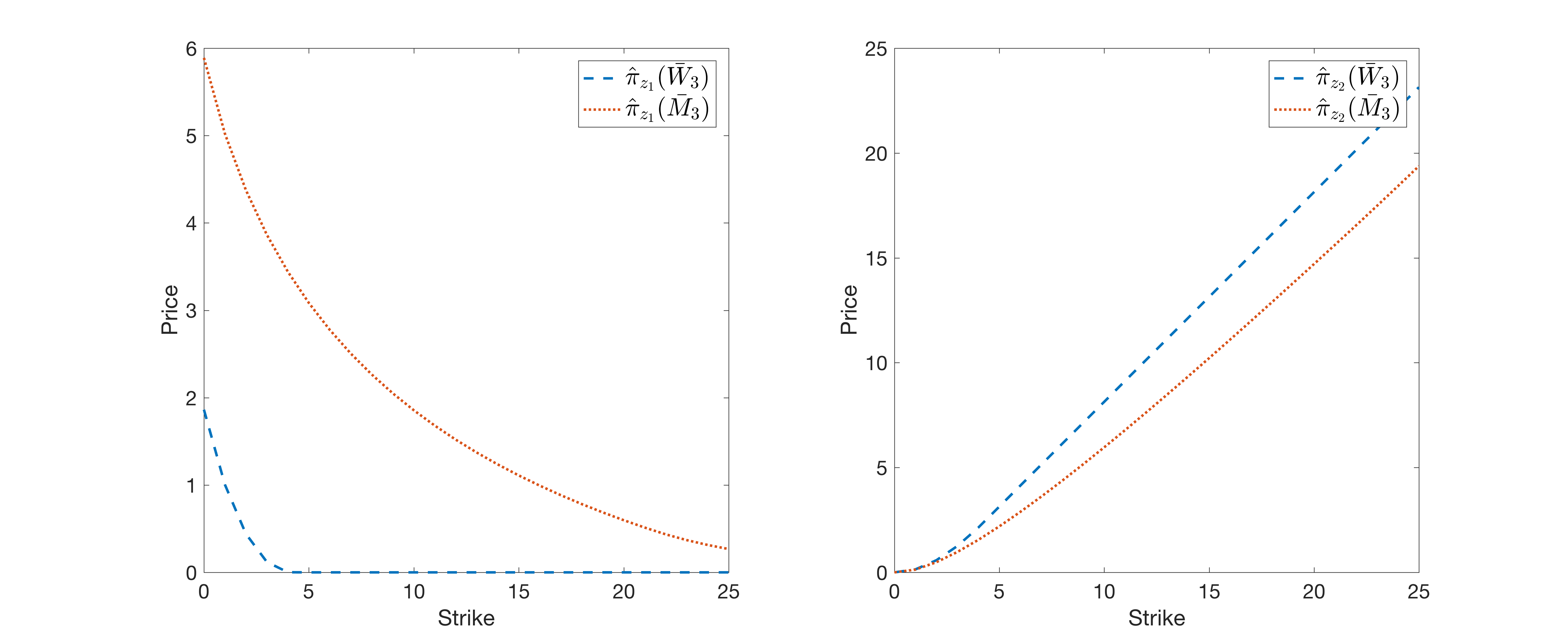
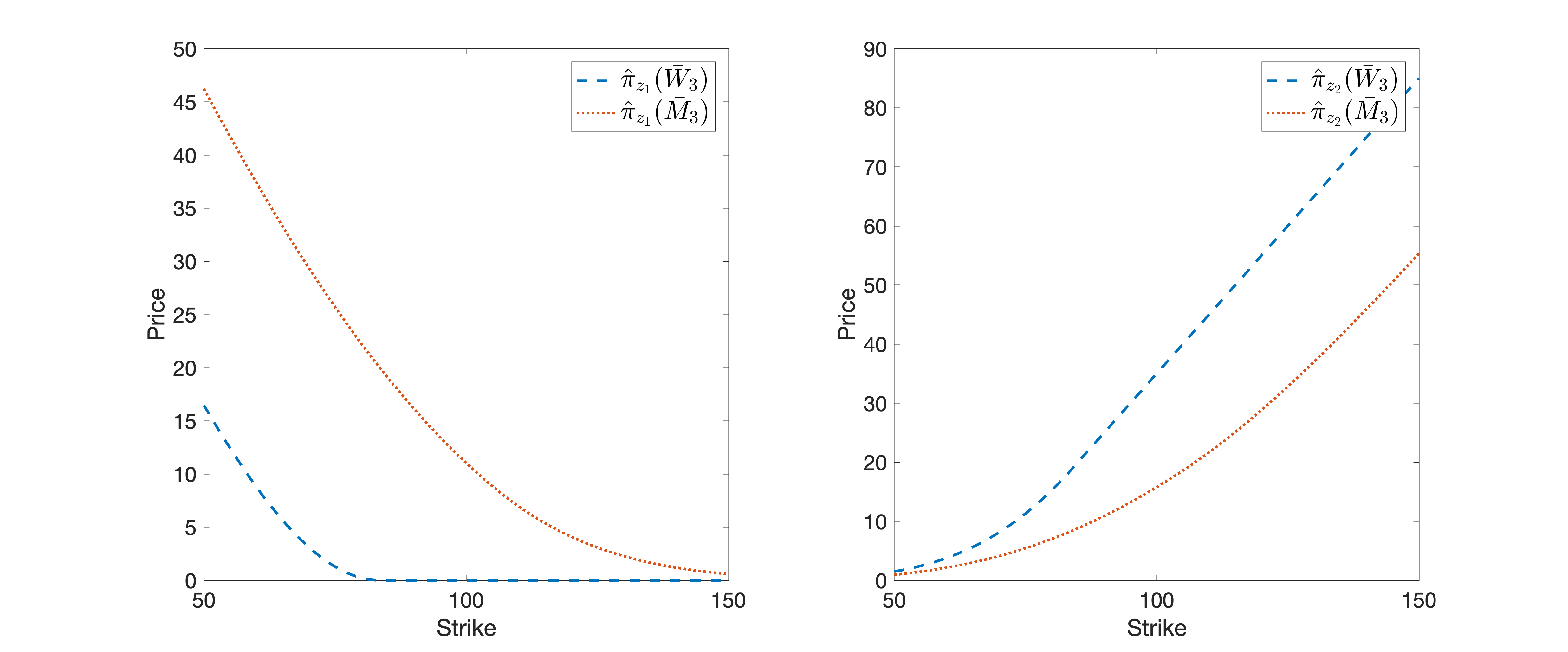
Refer to caption
Figure 1: Bounds for Π(Z1)Πsuperscript𝑍1\Pi(Z^{1}) (left) and Π(Z2)Πsuperscript𝑍2\Pi(Z^{2}) (right) derived by the Fréchet–Hoeffding bounds as a function of the strike; Setting 1.
Refer to caption
Figure 2: Bounds for Π(Z1)Πsuperscript𝑍1\Pi(Z^{1}) (left) and Π(Z2)Πsuperscript𝑍2\Pi(Z^{2}) (right) derived by the Fréchet–Hoeffding bounds as a function of the strike; Setting 2.
Remark 5.1.

Let us point out that the structure of the lower Fréchet–Hoeffding bound, together with the properties of the measures induced by the payoff functions, lead to some restrictions for the price bounds of put and call options on the minimum of several assets. Indeed, since W¯d(𝐮)=Wd(𝟏𝐮)subscript¯𝑊𝑑𝐮subscript𝑊𝑑1𝐮\overline{W}_{d}(\mathbf{u})=W_{d}(\mathbf{1}-\mathbf{u}) is decreasing in every uisubscript𝑢𝑖u_{i} and floored by 00, there exists an x0subscript𝑥0x_{0} such that W¯d(F1(x),,Fd(x))=0subscript¯𝑊𝑑subscript𝐹1𝑥subscript𝐹𝑑𝑥0\overline{W}_{d}\big{(}F_{1}(x),\dots,F_{d}(x)\big{)}=0 for x>x0𝑥subscript𝑥0x>x_{0}. This x0subscript𝑥0x_{0} depends on the marginal distributions. On the one hand, this yields for the lower bound of the call price that π^z1(W¯3)=0subscript^𝜋subscript𝑧1subscript¯𝑊30\widehat{\pi}_{z_{1}}(\overline{W}_{3})=0 for K1x0subscript𝐾1subscript𝑥0K_{1}\geq x_{0}; see also Figure 1 (where the price bounds are plotted as functions of the strike). On the other hand, for the upper bound of the put price, we get that π^z2(W¯3)=K2+csubscript^𝜋subscript𝑧2subscript¯𝑊3subscript𝐾2𝑐\widehat{\pi}_{z_{2}}(\overline{W}_{3})=K_{2}+c for K2x0subscript𝐾2subscript𝑥0K_{2}\geq x_{0} with constant c[0,x0]W¯3(F1(x),F2(x),F3(x))dx𝑐subscript0subscript𝑥0subscript¯𝑊3subscript𝐹1𝑥subscript𝐹2𝑥subscript𝐹3𝑥differential-d𝑥c\equiv\int_{[0,x_{0}]}\overline{W}_{3}\big{(}F_{1}(x),F_{2}(x),F_{3}(x)\big{)}\mathrm{d}x. There is no equivalent statement for the other two bounds πz1(M¯3)subscript𝜋subscript𝑧1subscript¯𝑀3\pi_{z_{1}}(\overline{M}_{3}) and πz2(M¯3)subscript𝜋subscript𝑧2subscript¯𝑀3\pi_{z_{2}}(\overline{M}_{3}) because, in general, Fi(x)<1subscript𝐹𝑖𝑥1F_{i}(x)<1 for x<𝑥x<\infty. \blacklozenge

5.2 Detecting an arbitrage

Finally, we present an application of the main result of this work, i.e. Theorem 4.14. More specifically, we detect an arbitrage in the market (S1,S2,S3,Z1,Z2)superscript𝑆1superscript𝑆2superscript𝑆3superscript𝑍1superscript𝑍2(S^{1},S^{2},S^{3},Z^{1},Z^{2}) that contains three assets and two three-asset derivatives, even though the prices of Z1superscript𝑍1Z^{1} and Z2superscript𝑍2Z^{2} lie inside their respective no-arbitrage bounds. Tavin [33] searches for the global minimum of the objective function fobj(𝐮):=Q¯𝐩(𝐮)Q¯𝐩(𝐮)assignsubscript𝑓obj𝐮subscript¯𝑄𝐩𝐮subscript¯𝑄𝐩𝐮f_{\mathrm{\mathrm{obj}}}(\mathbf{u}):=\overline{Q}_{\mathbf{p}}(\mathbf{u})-\underline{Q}_{\mathbf{p}}(\mathbf{u}) over the unit square. However, it suffices to find a 𝐮superscript𝐮\mathbf{u}^{*} such that fobj(𝐮)<0subscript𝑓objsuperscript𝐮0f_{\mathrm{obj}}(\mathbf{u}^{*})<0 and not necessarily the global minimum. Since we consider an additional dimension, we restrict ourselves to checking whether fobjsubscript𝑓objf_{\mathrm{obj}} becomes negative or not.

In Setting 1, we consider the call and put option on the minimum of three assets Z1superscript𝑍1Z^{1} and Z2superscript𝑍2Z^{2} with strikes K1=3subscript𝐾13K_{1}=3 and K2=8subscript𝐾28K_{2}=8 respectively. Then we have approximately the following no-arbitrage bounds:

Π(Z1)=[0.118,3.864]andΠ(Z2)=[4.374,6.138].formulae-sequenceΠsuperscript𝑍10.1183.864andΠsuperscript𝑍24.3746.138\displaystyle\Pi(Z^{1})=[0.118,3.864]\quad\text{and}\quad\Pi(Z^{2})=[4.374,6.138]\,.

Assume that the traded price for the call equals 3.53.53.5 and the traded price for the put equals 666, i.e. 𝐩=(3.5,6)𝐩3.56\mathbf{p}=(3.5,6). Obviously both prices lie within their respective no-arbitrage bounds, hence the two sub-markets where either Z1superscript𝑍1Z^{1} or Z2superscript𝑍2Z^{2} is the only multi-asset derivative are free of arbitrage. However, we numerically compute that

fobj(0.7,0.5,0.1)0.0952<0,subscript𝑓obj0.70.50.10.09520\displaystyle f_{\mathrm{obj}}(0.7,0.5,0.1)\approx-0.0952<0\,,

therefore Theorem 4.14 yields that the market with both multi-asset derivatives is not free of arbitrage, i.e. 𝐩Π(Z1,Z2)𝐩Πsuperscript𝑍1superscript𝑍2\mathbf{p}\notin\Pi(Z^{1},Z^{2}). Figure 3 shows a plot of the objective function fobjsubscript𝑓objf_{\mathrm{obj}}. One can see clearly how fobjsubscript𝑓objf_{\mathrm{obj}} drops below zero around 𝐮=(0.7,0.5,0.1)𝐮0.70.50.1\mathbf{u}=(0.7,0.5,0.1).

In Setting 2, we consider again the call and put option on the minimum of three assets Z1superscript𝑍1Z^{1} and Z2superscript𝑍2Z^{2} with strikes K1=60subscript𝐾160K_{1}=60 and K2=140subscript𝐾2140K_{2}=140 respectively. Then we have approximately the following no-arbitrage bounds:

Π(Z1)=[8.799,37.431]andΠ(Z2)=[45.94,75.018].formulae-sequenceΠsuperscript𝑍18.79937.431andΠsuperscript𝑍245.9475.018\displaystyle\Pi(Z^{1})=[8.799,37.431]\quad\text{and}\quad\Pi(Z^{2})=[45.94,75.018]\,.

Assume that the traded price for the call equals 999 and the traded price for the put equals 46.146.146.1, i.e. 𝐩=(9,46.1)𝐩946.1\mathbf{p}=(9,46.1). Obviously both prices lie within their respective no-arbitrage bounds, hence the two sub-markets where either Z1superscript𝑍1Z^{1} or Z2superscript𝑍2Z^{2} is the only multi-asset derivative are free of arbitrage. However, we numerically compute that

fobj(0.4,0.3,0.4)0.4905<0,subscript𝑓obj0.40.30.40.49050\displaystyle f_{\mathrm{obj}}(0.4,0.3,0.4)\approx-0.4905<0\,,

therefore Theorem 4.14 yields that the market with both multi-asset derivatives is not free of arbitrage, i.e. 𝐩Π(Z1,Z2)𝐩Πsuperscript𝑍1superscript𝑍2\mathbf{p}\notin\Pi(Z^{1},Z^{2}). Figure 4 shows a plot of the objective function fobjsubscript𝑓objf_{\mathrm{obj}}. One can see clearly how fobjsubscript𝑓objf_{\mathrm{obj}} drops below zero around 𝐮=(0.4,0.3,0.4)𝐮0.40.30.4\mathbf{u}=(0.4,0.3,0.4).

An intuitive explanation behind the appearance of arbitrage for the price vectors 𝐩=(3.5,6)𝐩3.56\mathbf{p}=(3.5,6), resp. 𝐩=(9,46.1)𝐩946.1\mathbf{p}=(9,46.1), could be as follows: The prices for Z1superscript𝑍1Z^{1} and Z2superscript𝑍2Z^{2} are both taken from the upper, resp. lower, part of the intervals Π(Z1)Πsuperscript𝑍1\Pi(Z^{1}) and Π(Z2)Πsuperscript𝑍2\Pi(Z^{2}); however, one payoff function is non-decreasing and the other is non- increasing with respect to the upper orthant order, which diminishes the possibility of finding a copula C𝐶C such that both π^z1(C^)=p1subscript^𝜋subscript𝑧1^𝐶subscript𝑝1\widehat{\pi}_{z_{1}}(\widehat{C})=p_{1} and π^z2(C^)=p2subscript^𝜋subscript𝑧2^𝐶subscript𝑝2\widehat{\pi}_{z_{2}}(\widehat{C})=p_{2} . A similar result in Setting 1 appears if we choose both prices close to the lower bounds; for example, for 𝐩=(0.3,4.5)𝐩0.34.5\mathbf{p}=(0.3,4.5) we get that

fobj(0.7,0.5,0.1)0.1257<0.subscript𝑓obj0.70.50.10.12570\displaystyle f_{\mathrm{obj}}(0.7,0.5,0.1)\approx-0.1257<0\,.

However, we have not noticed something analogous in Setting 2 when selecting both prices close to the upper bounds. On the other hand, if we select a price away from the upper bound for Z2superscript𝑍2Z^{2}, e.g. 𝐩=(3.5,4.5)𝐩3.54.5\mathbf{p}=(3.5,4.5) in Setting 1, then the objective function does not become negative any longer. Indeed, we find that the global minimum of the objective function fobjsubscript𝑓objf_{\mathrm{obj}} is zero, and is attained for ui=0subscript𝑢𝑖0u_{i}=0 or ui=1subscript𝑢𝑖1u_{i}=1 for some i=1,2,3𝑖123i=1,2,3, i.e. on the boundaries of the unit cube [0,1]3superscript013[0,1]^{3}. Let us point out again that this does not necessarily imply that the market is free of arbitrage, since Theorem 4.14 only provides a necessary condition.

(a)
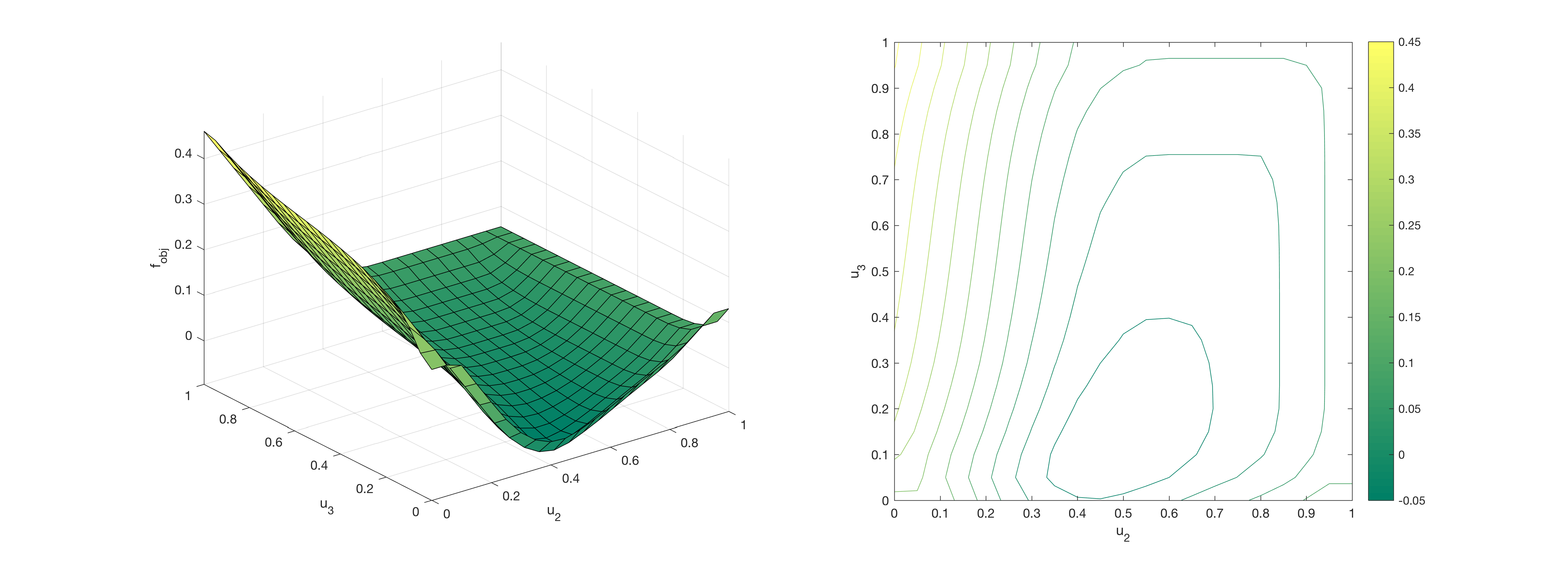
Refer to caption

(b)

Refer to caption

(c)

Refer to caption
Figure 3: Values and contour plots of the objective function fobjsubscript𝑓objf_{\mathrm{obj}} for 𝐩=(3.5,6)𝐩3.56\mathbf{p}=(3.5,6) and for the marginals restricted on (a) u1=0.7subscript𝑢10.7u_{1}=0.7, (b) u2=0.5subscript𝑢20.5u_{2}=0.5, (c) u3=0.1subscript𝑢30.1u_{3}=0.1; Setting 1.

(a)

Refer to caption

(b)

Refer to caption

(c)

Refer to caption
Figure 4: Values and contour plots of the objective function fobjsubscript𝑓objf_{\mathrm{obj}} for 𝐩=(9,46.1)𝐩946.1\mathbf{p}=(9,46.1) and for the marginals restricted on (a) u1=0.4subscript𝑢10.4u_{1}=0.4, (b) u2=0.3subscript𝑢20.3u_{2}=0.3, (c) u3=0.4subscript𝑢30.4u_{3}=0.4; Setting 2.

Appendix A Improved Fréchet–Hoeffding bounds for non-increasing functionals

The following two theorems cover the case when the map ρ𝜌\rho is non-increasing with respect to the orthant orders. This appears in our work when the negation of the payoff function, say ρ𝜌-\rho, is either ΔΔ\Delta-monotonic or ΔΔ\Delta-antitonic. In that case, we get that ρ(Md)ρ(Wd)𝜌subscript𝑀𝑑𝜌subscript𝑊𝑑\rho(M_{d})\leq\rho(W_{d}). The proofs of these results are omitted for the sake of brevity, as they are completely analogous to the proofs of Theorems 3.3 and A.2 in Lux and Papapantoleon [18].

Theorem A.1.

Let ρ:𝒬d:𝜌superscript𝒬𝑑\rho:\mathcal{Q}^{d}\rightarrow\mathbb{R} be non-increasing with respect to the lower orthant order and continuous with respect to the pointwise convergence of quasi-copulas. Let θ[ρ(Md),ρ(Wd)]𝜃𝜌subscript𝑀𝑑𝜌subscript𝑊𝑑\theta\in[\rho(M_{d}),\rho(W_{d})] and define

𝒬ρ,θ:={Q𝒬d|ρ(Q)=θ}.assignsuperscript𝒬𝜌𝜃conditional-set𝑄superscript𝒬𝑑𝜌𝑄𝜃\displaystyle\mathcal{Q}^{\rho,\theta}:=\big{\{}Q\in\mathcal{Q}^{d}\,|\,\rho(Q)=\theta\big{\}}\,.

Then, for all Q𝒬ρ,θ𝑄superscript𝒬𝜌𝜃Q\in\mathcal{Q}^{\rho,\theta}, holds

QLρ,θ(𝐮)Q(𝐮)QUρ,θ(𝐮)for all 𝐮[0,1]d,formulae-sequencesuperscriptsubscript𝑄𝐿𝜌𝜃𝐮𝑄𝐮superscriptsubscript𝑄𝑈𝜌𝜃𝐮for all 𝐮superscript01𝑑\displaystyle Q_{L}^{\rho,\theta}(\mathbf{u})\leq Q(\mathbf{u})\leq Q_{U}^{\rho,\theta}(\mathbf{u})\quad\textit{for all }\mathbf{u}\in[0,1]^{d}\,,

with

QLρ,θ(𝐮):=assignsuperscriptsubscript𝑄𝐿𝜌𝜃𝐮absent\displaystyle Q_{L}^{\rho,\theta}(\mathbf{u}):= {ρ+1(𝐮,θ),ifθ[ρ(Md),ρ+(𝐮,Wd(𝐮))],Md(𝐮),otherwise,casessubscriptsuperscript𝜌1𝐮𝜃if𝜃𝜌subscript𝑀𝑑subscript𝜌𝐮subscript𝑊𝑑𝐮otherwisesubscript𝑀𝑑𝐮otherwiseotherwise\displaystyle\begin{cases}\rho^{-1}_{+}(\mathbf{u},\theta)\,,\quad\textit{if}\,\,\theta\in[\rho(M_{d}),\rho_{+}(\mathbf{u},W_{d}(\mathbf{u}))],\\ M_{d}(\mathbf{u})\,,\quad\quad\textit{otherwise}\,,\end{cases}
QUρ,θ(𝐮):=assignsuperscriptsubscript𝑄𝑈𝜌𝜃𝐮absent\displaystyle Q_{U}^{\rho,\theta}(\mathbf{u}):= {ρ1(𝐮,θ),ifθ[ρ(𝐮,Md(𝐮)),ρ(Wd)],Wd(𝐮),otherwise.casessubscriptsuperscript𝜌1𝐮𝜃if𝜃subscript𝜌𝐮subscript𝑀𝑑𝐮𝜌subscript𝑊𝑑otherwisesubscript𝑊𝑑𝐮otherwiseotherwise\displaystyle\begin{cases}\rho^{-1}_{-}(\mathbf{u},\theta)\,,\quad\textit{if}\,\,\theta\in[\rho_{-}(\mathbf{u},M_{d}(\mathbf{u})),\rho(W_{d})],\\ W_{d}(\mathbf{u})\,,\quad\quad\textit{otherwise}.\end{cases}

\blacklozenge

Theorem A.2.

Let ρ:𝒞d:𝜌superscript𝒞𝑑\rho:\mathcal{C}^{d}\rightarrow\mathbb{R} be non-increasing with respect to the upper orthant order and continuous with respect to the pointwise convergence of copulas. Let θ[ρ^(M¯d),ρ^(W¯d)]𝜃^𝜌subscript¯𝑀𝑑^𝜌subscript¯𝑊𝑑\theta\in[\widehat{\rho}(\overline{M}_{d}),\widehat{\rho}(\overline{W}_{d})] and define

𝒞^ρ,θ:={C𝒞d|ρ^(C^)=θ}.assignsuperscript^𝒞𝜌𝜃conditional-set𝐶superscript𝒞𝑑^𝜌^𝐶𝜃\displaystyle\widehat{\mathcal{C}}^{\rho,\theta}:=\big{\{}C\in\mathcal{C}^{d}\,|\,\widehat{\rho}(\widehat{C})=\theta\big{\}}.

Then, for all C^𝒞^ρ,θ^𝐶superscript^𝒞𝜌𝜃\widehat{C}\in\widehat{\mathcal{C}}^{\rho,\theta}, holds

Q^Lρ,θ(𝐮)C^(𝐮)Q^Uρ,θ(𝐮)for all𝐮[0,1]d,formulae-sequencesuperscriptsubscript^𝑄𝐿𝜌𝜃𝐮^𝐶𝐮superscriptsubscript^𝑄𝑈𝜌𝜃𝐮for all𝐮superscript01𝑑\displaystyle\widehat{Q}_{L}^{\rho,\theta}(\mathbf{u})\leq\widehat{C}(\mathbf{u})\leq\widehat{Q}_{U}^{\rho,\theta}(\mathbf{u})\quad\textit{for all}\,\,\mathbf{u}\in[0,1]^{d}\,,

with

Q^Lρ,θ(𝐮):=assignsuperscriptsubscript^𝑄𝐿𝜌𝜃𝐮absent\displaystyle\widehat{Q}_{L}^{\rho,\theta}(\mathbf{u}):= {ρ^+1(𝐮,θ),ifθ[ρ^(M¯d),ρ^+(𝐮,W¯d(𝐮))],M¯d(𝐮),otherwise,casessubscriptsuperscript^𝜌1𝐮𝜃if𝜃^𝜌subscript¯𝑀𝑑subscript^𝜌𝐮subscript¯𝑊𝑑𝐮otherwisesubscript¯𝑀𝑑𝐮otherwiseotherwise\displaystyle\begin{cases}\widehat{\rho}^{\,-1}_{+}(\mathbf{u},\theta)\,,\quad\textit{if}\,\,\theta\in[\widehat{\rho}(\overline{M}_{d}),\widehat{\rho}_{+}(\mathbf{u},\overline{W}_{d}(\mathbf{u}))],\\ \overline{M}_{d}(\mathbf{u})\,,\quad\quad\textit{otherwise}\,,\end{cases}
Q^Uρ,θ(𝐮):=assignsuperscriptsubscript^𝑄𝑈𝜌𝜃𝐮absent\displaystyle\widehat{Q}_{U}^{\rho,\theta}(\mathbf{u}):= {ρ^1(𝐮,θ),ifθ[ρ^(𝐮,M¯d(𝐮)),ρ^(W¯d)],W¯d(𝐮),otherwise.casessubscriptsuperscript^𝜌1𝐮𝜃if𝜃subscript^𝜌𝐮subscript¯𝑀𝑑𝐮^𝜌subscript¯𝑊𝑑otherwisesubscript¯𝑊𝑑𝐮otherwise.otherwise\displaystyle\begin{cases}\widehat{\rho}^{\,-1}_{-}(\mathbf{u},\theta)\,,\quad\textit{if}\,\,\theta\in[\widehat{\rho}_{-}(\mathbf{u},\overline{M}_{d}(\mathbf{u})),\widehat{\rho}(\overline{W}_{d})],\\ \overline{W}_{d}(\mathbf{u})\,,\quad\quad\textit{otherwise.}\end{cases}

\blacklozenge

References

  • [1] D. Bartl, M. Kupper, T. Lux, A. Papapantoleon, and S. Eckstein. Marginal and dependence uncertainty: bounds, optimal transport, and sharpness. SIAM J. Control Optim. (forthcoming).
  • Bernard et al. [2012] C. Bernard, X. Jiang, and S. Vanduffel. A note on ‘Improved Fréchet bounds and model-free pricing of multi-asset options’ by Tankov (2011). J. Appl. Probab., 49:866–875, 2012.
  • Black and Scholes [1973] F. Black and M. Scholes. The pricing of options and corporate liabilities. J. Polit. Econ., 81:637–654, 1973.
  • Breeden and Litzenberger [1978] D. Breeden and R. Litzenberger. Prices of state-contingent claims implicit in options prices. J. Business, 51:621–651, 1978.
  • Buehler [2006] H. Buehler. Expensive martingales. Quant. Finance, 6(3):207–218, 2006.
  • Carr and Madan [2001] P. Carr and D. Madan. Optimal positioning in derivative securities. Quant. Finance, 1(1):19–37, 2001.
  • Carr and Madan [2005] P. Carr and D. Madan. A note on sufficient conditions for no arbitrage. Finance Res. Let., 2:125–130, 2005.
  • Cousot [2007] L. Cousot. Conditions on option prices for absence of arbitrage and exact calibration. J. Banking Finance, 31:3377–3397, 2007.
  • d’Aspremont and El Ghaoui [2006] A. d’Aspremont and L. El Ghaoui. Static arbitrage bounds on basket option prices. Math. Program., 106(3, Ser. A):467–489, 2006.
  • Davis and Hobson [2007] M. H. A. Davis and D. G. Hobson. The range of traded option prices. Math. Finance, 17:1–14, 2007.
  • Dhaene et al. [2002a] J. Dhaene, M. Denuit, M. J. Goovaerts, R. Kaas, and D. Vyncke. The concept of comonotonicity in actuarial science and finance: theory. Insurance Math. Econom., 31:3–33, 2002a.
  • Dhaene et al. [2002b] J. Dhaene, M. Denuit, M. J. Goovaerts, R. Kaas, and D. Vyncke. The concept of comonotonicity in actuarial science and finance: applications. Insurance Math. Econom., 31:133–161, 2002b.
  • Eberlein [2001] E. Eberlein. Application of generalized hyperbolic Lévy motions to finance. In O. E. Barndorff-Nielsen, T. Mikosch, and S. I. Resnick, editors, Lévy Processes: Theory and Applications, pages 319–336. Birkhäuser, 2001.
  • Gerhold and Gülüm [2020] S. Gerhold and I. C. Gülüm. Consistency of option prices under bid-ask spreads. Math. Finance, 30:377–402, 2020.
  • Hobson et al. [2005a] D. Hobson, P. Laurence, and T.-H. Wang. Static-arbitrage upper bounds for the prices of basket options. Quant. Finance, 5:329–342, 2005a.
  • Hobson et al. [2005b] D. Hobson, P. Laurence, and T.-H. Wang. Static-arbitrage optimal subreplicating strategies for basket options. Insurance Math. Econom., 37:553–572, 2005b.
  • Laurent and Leisen [2001] J.-P. Laurent and D. Leisen. Building a consistent pricing model from observed option prices. In M. Avellaneda, editor, Quantitative Analysis In Financial Markets: Collected Papers of the New York University Mathematical Finance Seminar (Volume II). World Scientific, 2001.
  • Lux and Papapantoleon [2017] T. Lux and A. Papapantoleon. Improved Fréchet–Hoeffding bounds on d𝑑d-copulas and applications in model-free finance. Ann. Appl. Probab., 27:3633–3671, 2017.
  • Lux and Papapantoleon [2019] T. Lux and A. Papapantoleon. Model-free bounds on Value-at-Risk using extreme value information and statistical distances. Insurance Math. Econom., 86:73–83, 2019.
  • Müller and Stoyan [2002] A. Müller and D. Stoyan. Comparison Methods for Stochastic Models and Risks. Wiley, 2002.
  • Nelsen [2006] R. B. Nelsen. An Introduction to Copulas. Springer, 2nd edition, 2006.
  • Neufeld et al. [2020] A. Neufeld, A. Papapantoleon, and Q. Xiang. Model-free bounds for multi-asset options using option-implied information and their exact computation. Preprint, arXiv:2006.14288, 2020.
  • Peña et al. [2010] J. Peña, J. C. Vera, and L. F. Zuluaga. Static-arbitrage lower bounds on the prices of basket options via linear programming. Quant. Finance, 10:819–827, 2010.
  • Puccetti et al. [2016] G. Puccetti, L. Rüschendorf, and D. Manko. VaR bounds for joint portfolios with dependence constraints. Depend. Model., 4:368–381, 2016.
  • Rachev and Rüschendorf [1994] S. T. Rachev and L. Rüschendorf. Solution of some transportation problems with relaxed or additional constraints. SIAM J. Control Optim., 32:673–689, 1994.
  • Rapuch and Roncalli [2004] G. Rapuch and T. Roncalli. Dependence and two-asset option pricing. J. Comput. Finance, 7(4):23–33, 2004.
  • Rüschendorf [1980] L. Rüschendorf. Inequalities for the expectation of ΔΔ\Delta-monotone functions. Z. Wahrsch. Verw. Gebiete, 54:341–349, 1980.
  • Rüschendorf [2004] L. Rüschendorf. Comparison of multivariate risks and positive dependence. J. Appl. Probab., 41:391–406, 2004.
  • Rüschendorf [2018] L. Rüschendorf. Risk bounds with additional information on functionals of the risk vector. Depend. Model., 6:102–113, 2018.
  • Sæbø [2009] K. K. Sæbø. Pricing exotic options with the normal inverse Gaussian market model using numerical path integration. Master’s thesis, NTNU, 2009.
  • Sklar [1959] M. Sklar. Fonctions de repartition a n𝑛n-dimensions et leurs marges. Publ. Inst. Statist. Univ. Paris, 8:229–231, 1959.
  • Tankov [2011] P. Tankov. Improved Fréchet bounds and model-free pricing of multi-asset options. J. Appl. Probab., 48:389–403, 2011.
  • Tavin [2015] B. Tavin. Detection of arbitrage in a market with multi-asset derivatives and known risk-neutral marginals. J. Banking Finance, 53:158–178, 2015.