Estimating Gradients for Discrete Random Variables by Sampling without Replacement

Wouter Kool
University of Amsterdam
ORTEC
w.w.m.kool@uva.nl
&Herke van Hoof
University of Amsterdam
h.c.vanhoof@uva.nl
&Max Welling
University of Amsterdam
CIFAR
m.welling@uva.nl
Abstract

We derive an unbiased estimator for expectations over discrete random variables based on sampling without replacement, which reduces variance as it avoids duplicate samples. We show that our estimator can be derived as the Rao-Blackwellization of three different estimators. Combining our estimator with REINFORCE, we obtain a policy gradient estimator and we reduce its variance using a built-in control variate which is obtained without additional model evaluations. The resulting estimator is closely related to other gradient estimators. Experiments with a toy problem, a categorical Variational Auto-Encoder and a structured prediction problem show that our estimator is the only estimator that is consistently among the best estimators in both high and low entropy settings.

1 Introduction

Put replacement in your basement! We derive the unordered set estimator111Code available at https://github.com/wouterkool/estimating-gradients-without-replacement.: an unbiased (gradient) estimator for expectations over discrete random variables based on (unordered sets of) samples without replacement. In particular, we consider the problem of estimating (the gradient of) the expectation of f​(𝒙)𝑓𝒙f(\bm{x}) where 𝒙𝒙\bm{x} has a discrete distribution p𝑝p over the domain D𝐷D, i.e.

π”Όπ’™βˆΌp​(𝒙)​[f​(𝒙)]=βˆ‘π’™βˆˆDp​(𝒙)​f​(𝒙).subscript𝔼similar-to𝒙𝑝𝒙delimited-[]𝑓𝒙subscript𝒙𝐷𝑝𝒙𝑓𝒙\mathbb{E}_{\bm{x}\sim p(\bm{x})}[f(\bm{x})]=\sum\nolimits_{\bm{x}\in D}p(\bm{x})f(\bm{x}). (1)

This expectation comes up in reinforcement learning, discrete latent variable modelling (e.g.Β for compression), structured prediction (e.g.Β for translation), hard attention and many other tasks that use models with discrete operations in their computational graphs (see e.g.Β Jang etΒ al. (2016)). In general, 𝒙𝒙\bm{x} has structure (such as a sequence), but we can treat it as a β€˜flat’ distribution, omitting the bold notation, so xπ‘₯x has a categorical distribution over D𝐷D given by p​(x),x∈D𝑝π‘₯π‘₯𝐷p(x),x\in D. Typically, the distribution has parameters 𝜽𝜽\bm{\theta}, which are learnt through gradient descent. This requires estimating the gradient βˆ‡πœ½π”Όx∼pπœ½β€‹(x)​[f​(x)]subscriptβˆ‡πœ½subscript𝔼similar-toπ‘₯subscriptπ‘πœ½π‘₯delimited-[]𝑓π‘₯\nabla_{\bm{\theta}}\mathbb{E}_{x\sim p_{\bm{\theta}}(x)}[f(x)], using a set of samples S𝑆S. A gradient estimate e​(S)𝑒𝑆e(S) is unbiased if

𝔼S​[e​(S)]=βˆ‡πœ½π”Όx∼pπœ½β€‹(x)​[f​(x)].subscript𝔼𝑆delimited-[]𝑒𝑆subscriptβˆ‡πœ½subscript𝔼similar-toπ‘₯subscriptπ‘πœ½π‘₯delimited-[]𝑓π‘₯\mathbb{E}_{S}[e(S)]=\nabla_{\bm{\theta}}\mathbb{E}_{x\sim p_{\bm{\theta}}(x)}[f(x)]. (2)

The samples S𝑆S can be sampled independently or using alternatives such as stratified sampling which reduce variance to increase the speed of learning. In this paper, we derive an unbiased gradient estimator that reduces variance by avoiding duplicate samples, i.e.Β by sampling S𝑆S without replacement. This is challenging as samples without replacement are dependent and have marginal distributions that are different from p​(x)𝑝π‘₯p(x). We further reduce the variance by deriving a built-in control variate, which maintains the unbiasedness and does not require additional samples.

Related work.

Many algorithms for estimating gradients for discrete distributions have been proposed. A general and widely used estimator is REINFORCE (Williams, 1992). Biased gradients based on a continuous relaxations of the discrete distribution (known as Gumbel-Softmax or Concrete) were jointly introduced by Jang etΒ al. (2016) and Maddison etΒ al. (2016). These can be combined with the straight through estimator (Bengio etΒ al., 2013) if the model requires discrete samples or be used to construct control variates for REINFORCE, as in REBAR (Tucker etΒ al., 2017) or RELAX (Grathwohl etΒ al., 2018). Many other methods use control variates and other techniques to reduce the variance of REINFORCE (Paisley etΒ al., 2012; Ranganath etΒ al., 2014; Gregor etΒ al., 2014; Mnih & Gregor, 2014; Gu etΒ al., 2016; Mnih & Rezende, 2016).

Some works rely on explicit summation of the expectation, either for the marginal distribution (Titsias & LΓ‘zaro-Gredilla, 2015) or globally summing some categories while sampling from the remainder (Liang etΒ al., 2018; Liu etΒ al., 2019). Other approaches use a finite difference approximation to the gradient (Lorberbom etΒ al., 2018; 2019). Yin etΒ al. (2019) introduced ARSM, which uses multiple model evaluations where the number adapts automatically to the uncertainty.

In the structured prediction setting, there are many algorithms for optimizing a quantity under a sequence of discrete decisions, using (weak) supervision, multiple samples (or deterministic model evaluations), or a combination both (Ranzato etΒ al., 2016; Shen etΒ al., 2016; He etΒ al., 2016; Norouzi etΒ al., 2016; Bahdanau etΒ al., 2017; Edunov etΒ al., 2018; Leblond etΒ al., 2018; Negrinho etΒ al., 2018). Most of these algorithms are biased and rely on pretraining using maximum likelihood or gradually transitioning from supervised to reinforcement learning. Using Gumbel-Softmax based approaches in a sequential setting is difficult as the bias accumulates because of mixing errors (Gu etΒ al., 2018).

2 Preliminaries

Throughout this paper, we will denote with Bksuperscriptπ΅π‘˜B^{k} an ordered sample without replacement of size kπ‘˜k and with Sksuperscriptπ‘†π‘˜S^{k} an unordered sample (of size kπ‘˜k) from the categorical distribution p𝑝p.

Restricted distribution.

When sampling without replacement, we remove the set CβŠ‚D𝐢𝐷C\subset D already sampled from the domain and we denote with pDβˆ–Csuperscript𝑝𝐷𝐢p^{D\setminus C} the distribution restricted to the domain Dβˆ–C𝐷𝐢D\setminus C:

pDβˆ–C​(x)=p​(x)1βˆ’βˆ‘c∈Cp​(c),x∈Dβˆ–C.formulae-sequencesuperscript𝑝𝐷𝐢π‘₯𝑝π‘₯1subscript𝑐𝐢𝑝𝑐π‘₯𝐷𝐢p^{D\setminus C}(x)=\frac{p(x)}{1-\sum_{c\in C}p(c)},\quad x\in D\setminus C. (3)
Ordered sample without replacement Bksuperscriptπ΅π‘˜B^{k}.

Let Bk=(b1,…,bk),bi∈Dformulae-sequencesuperscriptπ΅π‘˜subscript𝑏1…subscriptπ‘π‘˜subscript𝑏𝑖𝐷B^{k}=(b_{1},...,b_{k}),b_{i}\in D be an ordered sample without replacement, which is generated from the distribution p𝑝p as follows: first, sample b1∼psimilar-tosubscript𝑏1𝑝b_{1}\sim p, then sample b2∼pDβˆ–{b1}similar-tosubscript𝑏2superscript𝑝𝐷subscript𝑏1b_{2}\sim p^{D\setminus\{b_{1}\}}, b3∼pDβˆ–{b1,b2}similar-tosubscript𝑏3superscript𝑝𝐷subscript𝑏1subscript𝑏2b_{3}\sim p^{D\setminus\{b_{1},b_{2}\}}, etc.Β i.e.Β elements are sampled one by one without replacement. Using this procedure, Bksuperscriptπ΅π‘˜B^{k} can be seen as a (partial) ranking according to the Plackett-Luce model (Plackett, 1975; Luce, 1959) and the probability of obtaining the vector Bksuperscriptπ΅π‘˜B^{k} is

p​(Bk)=∏i=1kpDβˆ–Biβˆ’1​(bi)=∏i=1kp​(bi)1βˆ’βˆ‘j<ip​(bj).𝑝superscriptπ΅π‘˜superscriptsubscriptproduct𝑖1π‘˜superscript𝑝𝐷superscript𝐡𝑖1subscript𝑏𝑖superscriptsubscriptproduct𝑖1π‘˜π‘subscript𝑏𝑖1subscript𝑗𝑖𝑝subscript𝑏𝑗p(B^{k})=\prod_{i=1}^{k}p^{D\setminus B^{i-1}}(b_{i})=\prod_{i=1}^{k}\frac{p(b_{i})}{1-\sum\limits_{j<i}p(b_{j})}. (4)

We can also restrict Bksuperscriptπ΅π‘˜B^{k} to the domain Dβˆ–C𝐷𝐢D\setminus C, which means that biβˆ‰Csubscript𝑏𝑖𝐢b_{i}\not\in C for i=1,…,k𝑖1β€¦π‘˜i=1,...,k:

pDβˆ–C​(Bk)=∏i=1kpDβˆ–C​(bi)1βˆ’βˆ‘j<ipDβˆ–C​(bj)=∏i=1kp​(bi)1βˆ’βˆ‘c∈Cp​(c)βˆ’βˆ‘j<ip​(bj).superscript𝑝𝐷𝐢superscriptπ΅π‘˜superscriptsubscriptproduct𝑖1π‘˜superscript𝑝𝐷𝐢subscript𝑏𝑖1subscript𝑗𝑖superscript𝑝𝐷𝐢subscript𝑏𝑗superscriptsubscriptproduct𝑖1π‘˜π‘subscript𝑏𝑖1subscript𝑐𝐢𝑝𝑐subscript𝑗𝑖𝑝subscript𝑏𝑗p^{D\setminus C}(B^{k})=\prod_{i=1}^{k}\frac{p^{D\setminus C}(b_{i})}{1-\sum\limits_{j<i}p^{D\setminus C}(b_{j})}=\prod_{i=1}^{k}\frac{p(b_{i})}{1-\sum\limits_{c\in C}p(c)-\sum\limits_{j<i}p(b_{j})}. (5)
Unordered sample without replacement.

Let SkβŠ†Dsuperscriptπ‘†π‘˜π·S^{k}\subseteq D be an unordered sample without replacement from the distribution p𝑝p, which can be generated simply by generating an ordered sample and discarding the order. We denote elements in the sample with s∈Sk𝑠superscriptπ‘†π‘˜s\in S^{k} (so without index) and we write ℬ​(Sk)ℬsuperscriptπ‘†π‘˜\mathcal{B}(S^{k}) as the set of all k!π‘˜k! permutations (orderings) Bksuperscriptπ΅π‘˜B^{k} that correspond to (could have generated) Sksuperscriptπ‘†π‘˜S^{k}. It follows that the probability for sampling Sksuperscriptπ‘†π‘˜S^{k} is given by:

p​(Sk)=βˆ‘Bkβˆˆβ„¬β€‹(Sk)p​(Bk)=βˆ‘Bkβˆˆβ„¬β€‹(Sk)∏i=1kp​(bi)1βˆ’βˆ‘j<ip​(bj)=(∏s∈Skp​(s))β‹…βˆ‘Bkβˆˆβ„¬β€‹(Sk)∏i=1k11βˆ’βˆ‘j<ip​(bj).𝑝superscriptπ‘†π‘˜subscriptsuperscriptπ΅π‘˜β„¬superscriptπ‘†π‘˜π‘superscriptπ΅π‘˜subscriptsuperscriptπ΅π‘˜β„¬superscriptπ‘†π‘˜superscriptsubscriptproduct𝑖1π‘˜π‘subscript𝑏𝑖1subscript𝑗𝑖𝑝subscript𝑏𝑗⋅subscriptproduct𝑠superscriptπ‘†π‘˜π‘π‘ subscriptsuperscriptπ΅π‘˜β„¬superscriptπ‘†π‘˜superscriptsubscriptproduct𝑖1π‘˜11subscript𝑗𝑖𝑝subscript𝑏𝑗p(S^{k})=\sum_{B^{k}\in\mathcal{B}(S^{k})}p(B^{k})=\sum_{B^{k}\in\mathcal{B}(S^{k})}\prod_{i=1}^{k}\frac{p(b_{i})}{1-\sum\limits_{j<i}p(b_{j})}=\left(\prod_{s\in S^{k}}p(s)\right)\cdot\sum_{B^{k}\in\mathcal{B}(S^{k})}\prod_{i=1}^{k}\frac{1}{1-\sum\limits_{j<i}p(b_{j})}. (6)

The last step follows since Bkβˆˆβ„¬β€‹(Sk)superscriptπ΅π‘˜β„¬superscriptπ‘†π‘˜B^{k}\in\mathcal{B}(S^{k}) is an ordering of Sksuperscriptπ‘†π‘˜S^{k}, such that ∏i=1kp​(bi)=∏s∈Sp​(s)superscriptsubscriptproduct𝑖1π‘˜π‘subscript𝑏𝑖subscriptproduct𝑠𝑆𝑝𝑠\prod_{i=1}^{k}p(b_{i})=\prod_{s\in S}p(s). Naive computation of p​(Sk)𝑝superscriptπ‘†π‘˜p(S^{k}) is O​(k!)π‘‚π‘˜O(k!), but in Appendix B we show how to compute it efficiently.

When sampling from the distribution restricted to Dβˆ–C𝐷𝐢D\setminus C, we sample SkβŠ†Dβˆ–Csuperscriptπ‘†π‘˜π·πΆS^{k}\subseteq D\setminus C with probability:

pDβˆ–C​(Sk)=(∏s∈Skp​(s))β‹…βˆ‘Bkβˆˆβ„¬β€‹(Sk)∏i=1k11βˆ’βˆ‘c∈Cp​(c)βˆ’βˆ‘j<ip​(bj).superscript𝑝𝐷𝐢superscriptπ‘†π‘˜β‹…subscriptproduct𝑠superscriptπ‘†π‘˜π‘π‘ subscriptsuperscriptπ΅π‘˜β„¬superscriptπ‘†π‘˜superscriptsubscriptproduct𝑖1π‘˜11subscript𝑐𝐢𝑝𝑐subscript𝑗𝑖𝑝subscript𝑏𝑗p^{D\setminus C}(S^{k})=\left(\prod_{s\in S^{k}}p(s)\right)\cdot\sum_{B^{k}\in\mathcal{B}(S^{k})}\prod_{i=1}^{k}\frac{1}{1-\sum\limits_{c\in C}p(c)-\sum\limits_{j<i}p(b_{j})}. (7)
The Gumbel-Top-kπ‘˜k trick.

As an alternative to sequential sampling, we can also sample Bksuperscriptπ΅π‘˜B^{k} and Sksuperscriptπ‘†π‘˜S^{k} by taking the top kπ‘˜k of Gumbel variables (Yellott, 1977; Vieira, 2014; Kim etΒ al., 2016). Following notation from Kool etΒ al. (2019c), we define the perturbed log-probability gΟ•i=Ο•i+gisubscript𝑔subscriptitalic-ϕ𝑖subscriptitalic-ϕ𝑖subscript𝑔𝑖g_{\phi_{i}}=\phi_{i}+g_{i}, where Ο•i=log⁑p​(i)subscriptitalic-ϕ𝑖𝑝𝑖\phi_{i}=\log p(i) and gi∼Gumbel​(0)similar-tosubscript𝑔𝑖Gumbel0g_{i}\sim\text{Gumbel}(0). Then let b1=arg⁑maxi∈D⁑gΟ•isubscript𝑏1subscript𝑖𝐷subscript𝑔subscriptitalic-ϕ𝑖b_{1}=\arg\max_{i\in D}g_{\phi_{i}}, b2=arg⁑maxi∈Dβˆ–{b1}⁑gΟ•isubscript𝑏2subscript𝑖𝐷subscript𝑏1subscript𝑔subscriptitalic-ϕ𝑖b_{2}=\arg\max_{i\in D\setminus\{b_{1}\}}g_{\phi_{i}}, etc., so Bksuperscriptπ΅π‘˜B^{k} is the top kπ‘˜k of the perturbed log-probabilities in decreasing order. The probability of obtaining Bksubscriptπ΅π‘˜B_{k} using this procedure is given by equationΒ 4, so this provides an alternative sampling method which is effectively a (non-differentiable) reparameterization of sampling without replacement. For a differentiable reparameterization, see Grover etΒ al. (2019).

It follows that taking the top kπ‘˜k perturbed log-probabilities without order, we obtain the unordered sample set Sksuperscriptπ‘†π‘˜S^{k}. This way of sampling underlies the efficient computation of p​(Sk)𝑝superscriptπ‘†π‘˜p(S^{k}) in Appendix B.

3 Methodology

In this section, we derive the unordered set policy gradient estimator: a low-variance, unbiased estimator of βˆ‡πœ½π”Όpπœ½β€‹(x)​[f​(x)]subscriptβˆ‡πœ½subscript𝔼subscriptπ‘πœ½π‘₯delimited-[]𝑓π‘₯\nabla_{\bm{\theta}}\mathbb{E}_{p_{\bm{\theta}}(x)}[f(x)] based on an unordered sample without replacement Sksuperscriptπ‘†π‘˜S^{k}. First, we derive the generic (non-gradient) estimator for 𝔼​[f​(x)]𝔼delimited-[]𝑓π‘₯\mathbb{E}[f(x)] as the Rao-Blackwellized version of a single sample Monte Carlo estimator (and two other estimators!). Then we combine this estimator with REINFORCE (Williams, 1992) and we show how to reduce its variance using a built-in baseline.

3.1 Rao-Blackwellization of the single sample estimator

A very crude but simple estimator for 𝔼​[f​(x)]𝔼delimited-[]𝑓π‘₯\mathbb{E}[f(x)] based on the ordered sample Bksuperscriptπ΅π‘˜B^{k} is to only use the first element b1subscript𝑏1b_{1}, which by definition is a sample from the distribution p𝑝p. We define this estimator as the single sample estimator, which is unbiased, since

𝔼Bk∼p​(Bk)​[f​(b1)]=𝔼b1∼p​(b1)​[f​(b1)]=𝔼x∼p​(x)​[f​(x)].subscript𝔼similar-tosuperscriptπ΅π‘˜π‘superscriptπ΅π‘˜delimited-[]𝑓subscript𝑏1subscript𝔼similar-tosubscript𝑏1𝑝subscript𝑏1delimited-[]𝑓subscript𝑏1subscript𝔼similar-toπ‘₯𝑝π‘₯delimited-[]𝑓π‘₯\mathbb{E}_{B^{k}\sim p(B^{k})}[f(b_{1})]=\mathbb{E}_{b_{1}\sim p(b_{1})}[f(b_{1})]=\mathbb{E}_{x\sim p(x)}[f(x)]. (8)

Discarding all but one sample, the single sample estimator is inefficient, but we can use Rao-Blackwellization (Casella & Robert, 1996) to signficantly improve it. To this end, we consider the distribution Bk|Skconditionalsuperscriptπ΅π‘˜superscriptπ‘†π‘˜B^{k}|S^{k}, which is, knowing the unordered sample Sksuperscriptπ‘†π‘˜S^{k}, the conditional distribution over ordered samples Bkβˆˆβ„¬β€‹(Sk)superscriptπ΅π‘˜β„¬superscriptπ‘†π‘˜B^{k}\in\mathcal{B}(S^{k}) that could have generated Sksuperscriptπ‘†π‘˜S^{k}.222Note that Bk|Skconditionalsuperscriptπ΅π‘˜superscriptπ‘†π‘˜B^{k}|S^{k} is not a Plackett-Luce distribution restricted to Sksuperscriptπ‘†π‘˜S^{k}! Using Bk|Skconditionalsuperscriptπ΅π‘˜superscriptπ‘†π‘˜B^{k}|S^{k}, we rewrite 𝔼​[f​(b1)]𝔼delimited-[]𝑓subscript𝑏1\mathbb{E}[f(b_{1})] as

𝔼Bk∼p​(Bk)​[f​(b1)]=𝔼Sk∼p​(Sk)​[𝔼Bk∼p​(Bk|Sk)​[f​(b1)]]=𝔼Sk∼p​(Sk)​[𝔼b1∼p​(b1|Sk)​[f​(b1)]].subscript𝔼similar-tosuperscriptπ΅π‘˜π‘superscriptπ΅π‘˜delimited-[]𝑓subscript𝑏1subscript𝔼similar-tosuperscriptπ‘†π‘˜π‘superscriptπ‘†π‘˜delimited-[]subscript𝔼similar-tosuperscriptπ΅π‘˜π‘conditionalsuperscriptπ΅π‘˜superscriptπ‘†π‘˜delimited-[]𝑓subscript𝑏1subscript𝔼similar-tosuperscriptπ‘†π‘˜π‘superscriptπ‘†π‘˜delimited-[]subscript𝔼similar-tosubscript𝑏1𝑝conditionalsubscript𝑏1superscriptπ‘†π‘˜delimited-[]𝑓subscript𝑏1\mathbb{E}_{B^{k}\sim p(B^{k})}[f(b_{1})]=\mathbb{E}_{S^{k}\sim p(S^{k})}\left[\mathbb{E}_{B^{k}\sim p(B^{k}|S^{k})}\left[f(b_{1})\right]\right]=\mathbb{E}_{S^{k}\sim p(S^{k})}\left[\mathbb{E}_{b_{1}\sim p(b_{1}|S^{k})}\left[f(b_{1})\right]\right].

The Rao-Blackwellized version of the single sample estimator computes the inner conditional expectation exactly. Since Bksuperscriptπ΅π‘˜B^{k} is an ordering of Sksuperscriptπ‘†π‘˜S^{k}, we have b1∈Sksubscript𝑏1superscriptπ‘†π‘˜b_{1}\in S^{k} and we can compute this as

𝔼b1∼p​(b1|Sk)​[f​(b1)]=βˆ‘s∈SkP​(b1=s|Sk)​f​(s)subscript𝔼similar-tosubscript𝑏1𝑝conditionalsubscript𝑏1superscriptπ‘†π‘˜delimited-[]𝑓subscript𝑏1subscript𝑠superscriptπ‘†π‘˜π‘ƒsubscript𝑏1conditional𝑠superscriptπ‘†π‘˜π‘“π‘ \mathbb{E}_{b_{1}\sim p(b_{1}|S^{k})}\left[f(b_{1})\right]=\sum_{s\in S^{k}}P(b_{1}=s|S^{k})f(s) (9)

where, in a slight abuse of notation, P​(b1=s|Sk)𝑃subscript𝑏1conditional𝑠superscriptπ‘†π‘˜P(b_{1}=s|S^{k}) is the probability that the first sampled element b1subscript𝑏1b_{1} takes the value s𝑠s, given that the complete set of kπ‘˜k samples is Sksuperscriptπ‘†π‘˜S^{k}. Using Bayes’ Theorem we find

P​(b1=s|Sk)=p​(Sk|b1=s)​P​(b1=s)p​(Sk)=pDβˆ–{s}​(Skβˆ–{s})​p​(s)p​(Sk).𝑃subscript𝑏1conditional𝑠superscriptπ‘†π‘˜π‘conditionalsuperscriptπ‘†π‘˜subscript𝑏1𝑠𝑃subscript𝑏1𝑠𝑝superscriptπ‘†π‘˜superscript𝑝𝐷𝑠superscriptπ‘†π‘˜π‘ π‘π‘ π‘superscriptπ‘†π‘˜P(b_{1}=s|S^{k})=\frac{p(S^{k}|b_{1}=s)P(b_{1}=s)}{p(S^{k})}=\frac{p^{D\setminus\{s\}}(S^{k}\setminus\{s\})p(s)}{p(S^{k})}. (10)

The step p​(Sk|b1=s)=pDβˆ–{s}​(Skβˆ–{s})𝑝conditionalsuperscriptπ‘†π‘˜subscript𝑏1𝑠superscript𝑝𝐷𝑠superscriptπ‘†π‘˜π‘ p(S^{k}|b_{1}=s)=p^{D\setminus\{s\}}(S^{k}\setminus\{s\}) comes from analyzing sequential sampling without replacement: given that the first element sampled is s𝑠s, the remaining elements have a distribution restricted to Dβˆ–{s}𝐷𝑠D\setminus\{s\}, so sampling Sksuperscriptπ‘†π‘˜S^{k} (including s𝑠s) given the first element s𝑠s is equivalent to sampling the remainder Skβˆ–{s}superscriptπ‘†π‘˜π‘ S^{k}\setminus\{s\} from the restricted distribution, which has probability pDβˆ–{s}​(Skβˆ–{s})superscript𝑝𝐷𝑠superscriptπ‘†π‘˜π‘ p^{D\setminus\{s\}}(S^{k}\setminus\{s\}) (see equationΒ 7).

The unordered set estimator.

For notational convenience, we introduce the leave-one-out ratio.

Definition 1.

The leave-one-out ratio of s𝑠s w.r.t.Β the set S𝑆S is given by R​(Sk,s)=pDβˆ–{s}​(Skβˆ–{s})p​(Sk)𝑅superscriptπ‘†π‘˜π‘ superscript𝑝𝐷𝑠superscriptπ‘†π‘˜π‘ π‘superscriptπ‘†π‘˜R(S^{k},s)=\frac{p^{D\setminus\{s\}}(S^{k}\setminus\{s\})}{p(S^{k})}.

Rewriting equationΒ 10 as P​(b1=s|Sk)=p​(s)​R​(Sk,s)𝑃subscript𝑏1conditional𝑠superscriptπ‘†π‘˜π‘π‘ π‘…superscriptπ‘†π‘˜π‘ P(b_{1}=s|S^{k})=p(s)R(S^{k},s) shows that the probability of sampling s𝑠s first, given Sksuperscriptπ‘†π‘˜S^{k}, is simply the unconditional probability multiplied by the leave-one-out ratio. We now define the unordered set estimator as the Rao-Blackwellized version of the single-sample estimator.

Theorem 1.

The unordered set estimator, given by

eUS​(Sk)=βˆ‘s∈Skp​(s)​R​(Sk,s)​f​(s)superscript𝑒USsuperscriptπ‘†π‘˜subscript𝑠superscriptπ‘†π‘˜π‘π‘ π‘…superscriptπ‘†π‘˜π‘ π‘“π‘ e^{\text{US}}(S^{k})=\sum_{s\in S^{k}}p(s)R(S^{k},s)f(s) (11)

is the Rao-Blackwellized version of the (unbiased!) single sample estimator.

Proof.

Using P​(b1=s|Sk)=p​(s)​R​(Sk,s)𝑃subscript𝑏1conditional𝑠superscriptπ‘†π‘˜π‘π‘ π‘…superscriptπ‘†π‘˜π‘ P(b_{1}=s|S^{k})=p(s)R(S^{k},s) in equationΒ 9 we have

𝔼b1∼p​(b1|Sk)​[f​(b1)]=βˆ‘s∈SkP​(b1=s|Sk)​f​(s)=βˆ‘s∈Skp​(s)​R​(Sk,s)​f​(s).subscript𝔼similar-tosubscript𝑏1𝑝conditionalsubscript𝑏1superscriptπ‘†π‘˜delimited-[]𝑓subscript𝑏1subscript𝑠superscriptπ‘†π‘˜π‘ƒsubscript𝑏1conditional𝑠superscriptπ‘†π‘˜π‘“π‘ subscript𝑠superscriptπ‘†π‘˜π‘π‘ π‘…superscriptπ‘†π‘˜π‘ π‘“π‘ \mathbb{E}_{b_{1}\sim p(b_{1}|S^{k})}\left[f(b_{1})\right]=\sum_{s\in S^{k}}P(b_{1}=s|S^{k})f(s)=\sum_{s\in S^{k}}p(s)R(S^{k},s)f(s). (12)

∎

The implication of this theorem is that the unordered set estimator, in explicit form given by equationΒ 11, is an unbiased estimator of 𝔼​[f​(x)]𝔼delimited-[]𝑓π‘₯\mathbb{E}[f(x)] since it is the Rao-Blackwellized version of the unbiased single sample estimator. Also, as expected by taking multiple samples, it has variance equal or lower than the single sample estimator by the Rao-Blackwell Theorem (Lehmann & ScheffΓ©, 1950).

3.2 Rao-Blackwellization of other estimators

The unordered set estimator is also the result of Rao-Blackwellizing two other unbiased estimators: the stochastic sum-and-sample estimator and the importance-weighted estimator.

The sum-and-sample estimator.

We define as sum-and-sample estimator any estimator that relies on the identity that for any CβŠ‚D𝐢𝐷C\subset D

𝔼x∼p​(x)​[f​(x)]=𝔼x∼pDβˆ–C​(x)​[βˆ‘c∈Cp​(c)​f​(c)+(1βˆ’βˆ‘c∈Cp​(c))​f​(x)].subscript𝔼similar-toπ‘₯𝑝π‘₯delimited-[]𝑓π‘₯subscript𝔼similar-toπ‘₯superscript𝑝𝐷𝐢π‘₯delimited-[]subscript𝑐𝐢𝑝𝑐𝑓𝑐1subscript𝑐𝐢𝑝𝑐𝑓π‘₯\mathbb{E}_{x\sim p(x)}[f(x)]=\mathbb{E}_{x\sim p^{D\setminus C}(x)}\left[\sum_{c\in C}p(c)f(c)+\left(1-\sum_{c\in C}p(c)\right)f(x)\right]. (13)

For the derivation, see Appendix C.1 or Liang etΒ al. (2018); Liu etΒ al. (2019). In general, a sum-and-sample estimator with a budget of k>1π‘˜1k>1 evaluations sums expectation terms for a set of categories C𝐢C (s.t. |C|<kπΆπ‘˜|C|<k) explicitly (e.g.Β selected by their value f𝑓f (Liang etΒ al., 2018) or probability p𝑝p (Liu etΒ al., 2019)), and uses kβˆ’|C|π‘˜πΆk-|C| (down-weighted) samples from Dβˆ–C𝐷𝐢D\setminus C to estimate the remaining terms. As is noted by Liu etΒ al. (2019), selecting C𝐢C such that 1βˆ’βˆ‘c∈Cp​(c)kβˆ’|C|1subscriptπ‘πΆπ‘π‘π‘˜πΆ\frac{1-\sum_{c\in C}p(c)}{k-|C|} is minimized guarantees to reduce variance compared to a standard minibatch of kπ‘˜k samples (which is equivalent to setting C=βˆ…πΆC=\emptyset). See also Fearnhead & Clifford (2003) for a discussion on selecting C𝐢C optimally. The ability to optimize C𝐢C depends on whether p​(c)𝑝𝑐p(c) can be computed efficiently a-priori (before sampling). This is difficult in high-dimensional settings, e.g.Β sequence models which compute the probability incrementally while ancestral sampling. An alternative is to select C𝐢C stochastically (as equationΒ 13 holds for any C𝐢C), and we choose C=Bkβˆ’1𝐢superscriptπ΅π‘˜1C=B^{k-1} to define the stochastic sum-and-sample estimator:

eSSAS​(Bk)=βˆ‘j=1kβˆ’1p​(bj)​f​(bj)+(1βˆ’βˆ‘j=1kβˆ’1p​(bj))​f​(bk).superscript𝑒SSASsuperscriptπ΅π‘˜superscriptsubscript𝑗1π‘˜1𝑝subscript𝑏𝑗𝑓subscript𝑏𝑗1superscriptsubscript𝑗1π‘˜1𝑝subscript𝑏𝑗𝑓subscriptπ‘π‘˜e^{\text{SSAS}}(B^{k})=\sum_{j=1}^{k-1}p(b_{j})f(b_{j})+\left(1-\sum_{j=1}^{k-1}p(b_{j})\right)f(b_{k}). (14)

For simplicity, we consider the version that sums kβˆ’1π‘˜1k-1 terms here, but the following results also hold for a version that sums kβˆ’mπ‘˜π‘šk-m terms and uses mπ‘šm samples (without replacement) (see Appendix C.3). Sampling without replacement, it holds that bk|Bkβˆ’1∼pDβˆ–Bkβˆ’1similar-toconditionalsubscriptπ‘π‘˜superscriptπ΅π‘˜1superscript𝑝𝐷superscriptπ΅π‘˜1b_{k}|B^{k-1}\sim p^{D\setminus B^{k-1}}, so the unbiasedness follows from equationΒ 13 by separating the expectation over Bksuperscriptπ΅π‘˜B^{k} into expectations over Bkβˆ’1superscriptπ΅π‘˜1B^{k-1} and bk|Bkβˆ’1conditionalsubscriptπ‘π‘˜superscriptπ΅π‘˜1b_{k}|B^{k-1}:

𝔼Bkβˆ’1∼p​(Bkβˆ’1)​[𝔼bk∼p​(bk|Bkβˆ’1)​[eSSAS​(Bk)]]=𝔼Bkβˆ’1∼p​(Bkβˆ’1)​[𝔼​[f​(x)]]=𝔼​[f​(x)].subscript𝔼similar-tosuperscriptπ΅π‘˜1𝑝superscriptπ΅π‘˜1delimited-[]subscript𝔼similar-tosubscriptπ‘π‘˜π‘conditionalsubscriptπ‘π‘˜superscriptπ΅π‘˜1delimited-[]superscript𝑒SSASsuperscriptπ΅π‘˜subscript𝔼similar-tosuperscriptπ΅π‘˜1𝑝superscriptπ΅π‘˜1delimited-[]𝔼delimited-[]𝑓π‘₯𝔼delimited-[]𝑓π‘₯\mathbb{E}_{B^{k-1}\sim p(B^{k-1})}\left[\mathbb{E}_{b_{k}\sim p(b_{k}|B^{k-1})}\left[e^{\text{SSAS}}(B^{k})\right]\right]\\ =\mathbb{E}_{B^{k-1}\sim p(B^{k-1})}\left[\mathbb{E}[f(x)]\right]\\ =\mathbb{E}[f(x)].\\

In general, a sum-and-sample estimator reduces variance if the probability mass is concentrated on the summed categories. As typically high probability categories are sampled first, the stochastic sum-and-sample estimator sums high probability categories, similar to the estimator by Liu etΒ al. (2019) which we refer to as the deterministic sum-and-sample estimator. As we show in Appendix C.2, Rao-Blackwellizing the stochastic sum-and-sample estimator also results in the unordered set estimator. This even holds for a version that uses mπ‘šm samples and kβˆ’mπ‘˜π‘šk-m summed terms (see Appendix C.3), which means that the unordered set estimator has equal or lower variance than the optimal (in terms of mπ‘šm) stochastic sum-and-sample estimator, but conveniently does not need to choose mπ‘šm.

The importance-weighted estimator.

The importance-weighted estimator (Vieira, 2017) is

eIW​(Sk,ΞΊ)=βˆ‘s∈Skp​(s)q​(s,ΞΊ)​f​(s).superscript𝑒IWsuperscriptπ‘†π‘˜πœ…subscript𝑠superscriptπ‘†π‘˜π‘π‘ π‘žπ‘ πœ…π‘“π‘ e^{\text{IW}}(S^{k},\kappa)=\sum_{s\in S^{k}}\frac{p(s)}{q(s,\kappa)}f(s). (15)

This estimator is based on the idea of priority sampling (Duffield etΒ al., 2007). It does not use the order of the sample, but assumes sampling using the Gumbel-Top-kπ‘˜k trick and requires access to ΞΊπœ…\kappa, the (k+1)π‘˜1(k+1)-th largest perturbed log-probability, which can be seen as the β€˜threshold’ since gΟ•s>ΞΊβ€‹βˆ€s∈Sksubscript𝑔subscriptitalic-Ο•π‘ πœ…for-all𝑠superscriptπ‘†π‘˜g_{\phi_{s}}>\kappa\;\forall s\in S^{k}. q​(s,a)=P​(gΟ•s>a)π‘žπ‘ π‘Žπ‘ƒsubscript𝑔subscriptitalic-Ο•π‘ π‘Žq(s,a)=P(g_{\phi_{s}}>a) can be interpreted as the inclusion probability of s∈Sk𝑠superscriptπ‘†π‘˜s\in S^{k} (assuming a fixed threshold aπ‘Ža instead of a fixed sample size kπ‘˜k). For details and a proof of unbiasedness, see Vieira (2017) or Kool etΒ al. (2019c). As the estimator has high variance, Kool etΒ al. (2019c) resort to normalizing the importance weights, resulting in biased estimates. Instead, we use Rao-Blackwellization to eliminate stochasticity by ΞΊπœ…\kappa. Again, the result is the unordered set estimator (see Appendix D.1), which thus has equal or lower variance.

3.3 The unordered set policy gradient estimator

Writing p𝜽subscriptπ‘πœ½p_{\bm{\theta}} to indicate the dependency on the model parameters 𝜽𝜽\bm{\theta}, we can combine the unordered set estimator with REINFORCE (Williams, 1992) to obtain the unordered set policy gradient estimator.

Corollary 1.

The unordered set policy gradient estimator, given by

eUSPG​(Sk)=βˆ‘s∈Skpπœ½β€‹(s)​R​(Sk,s)β€‹βˆ‡πœ½log⁑pπœ½β€‹(s)​f​(s)=βˆ‘s∈Skβˆ‡πœ½pπœ½β€‹(s)​R​(Sk,s)​f​(s),superscript𝑒USPGsuperscriptπ‘†π‘˜subscript𝑠superscriptπ‘†π‘˜subscriptπ‘πœ½π‘ π‘…superscriptπ‘†π‘˜π‘ subscriptβˆ‡πœ½subscriptπ‘πœ½π‘ π‘“π‘ subscript𝑠superscriptπ‘†π‘˜subscriptβˆ‡πœ½subscriptπ‘πœ½π‘ π‘…superscriptπ‘†π‘˜π‘ π‘“π‘ e^{\text{USPG}}(S^{k})=\sum_{s\in S^{k}}p_{\bm{\theta}}(s)R(S^{k},s)\nabla_{\bm{\theta}}\log p_{\bm{\theta}}(s)f(s)=\sum_{s\in S^{k}}\nabla_{\bm{\theta}}p_{\bm{\theta}}(s)R(S^{k},s)f(s), (16)

is an unbiased estimate of the policy gradient.

Proof.

Using REINFORCE (Williams, 1992) combined with the unordered set estimator we find:

βˆ‡πœ½π”Όpπœ½β€‹(x)​[f​(x)]=𝔼pπœ½β€‹(x)​[βˆ‡πœ½log⁑pπœ½β€‹(x)​f​(x)]=𝔼Sk∼pπœ½β€‹(Sk)​[βˆ‘s∈Skpπœ½β€‹(s)​R​(Sk,s)β€‹βˆ‡πœ½log⁑pπœ½β€‹(s)​f​(s)].subscriptβˆ‡πœ½subscript𝔼subscriptπ‘πœ½π‘₯delimited-[]𝑓π‘₯subscript𝔼subscriptπ‘πœ½π‘₯delimited-[]subscriptβˆ‡πœ½subscriptπ‘πœ½π‘₯𝑓π‘₯subscript𝔼similar-tosuperscriptπ‘†π‘˜subscriptπ‘πœ½superscriptπ‘†π‘˜delimited-[]subscript𝑠superscriptπ‘†π‘˜subscriptπ‘πœ½π‘ π‘…superscriptπ‘†π‘˜π‘ subscriptβˆ‡πœ½subscriptπ‘πœ½π‘ π‘“π‘ \nabla_{\bm{\theta}}\mathbb{E}_{p_{\bm{\theta}}(x)}[f(x)]=\mathbb{E}_{p_{\bm{\theta}}(x)}[\nabla_{\bm{\theta}}\log p_{\bm{\theta}}(x)f(x)]=\mathbb{E}_{S^{k}\sim p_{\bm{\theta}}(S^{k})}\left[\sum_{s\in S^{k}}p_{\bm{\theta}}(s)R(S^{k},s)\nabla_{\bm{\theta}}\log p_{\bm{\theta}}(s)f(s)\right].

∎

Variance reduction using a built-in control variate.

The variance of REINFORCE can be reduced by subtracting a baseline from f𝑓f. When taking multiple samples (with replacement), a simple and effective baseline is to take the mean of other (independent!) samples (Mnih & Rezende, 2016). Sampling without replacement, we can use the same idea to construct a baseline based on the other samples, but we have to correct for the fact that the samples are not independent.

Theorem 2.

The unordered set policy gradient estimator with baseline, given by

eUSPGBL​(Sk)=βˆ‘s∈Skβˆ‡πœ½pπœ½β€‹(s)​R​(Sk,s)​(f​(s)βˆ’βˆ‘sβ€²βˆˆSkpπœ½β€‹(sβ€²)​RDβˆ–{s}​(Sk,sβ€²)​f​(sβ€²)),superscript𝑒USPGBLsuperscriptπ‘†π‘˜subscript𝑠superscriptπ‘†π‘˜subscriptβˆ‡πœ½subscriptπ‘πœ½π‘ π‘…superscriptπ‘†π‘˜π‘ π‘“π‘ subscriptsuperscript𝑠′superscriptπ‘†π‘˜subscriptπ‘πœ½superscript𝑠′superscript𝑅𝐷𝑠superscriptπ‘†π‘˜superscript𝑠′𝑓superscript𝑠′e^{\text{USPGBL}}(S^{k})=\sum_{s\in S^{k}}\nabla_{\bm{\theta}}p_{\bm{\theta}}(s)R(S^{k},s)\left(f(s)-\sum_{s^{\prime}\in S^{k}}p_{\bm{\theta}}(s^{\prime})R^{D\setminus\{s\}}(S^{k},s^{\prime})f(s^{\prime})\right), (17)

where

RDβˆ–{s}​(Sk,sβ€²)=p𝜽Dβˆ–{s,sβ€²}​(Skβˆ–{s,sβ€²})p𝜽Dβˆ–{s}​(Skβˆ–{s})superscript𝑅𝐷𝑠superscriptπ‘†π‘˜superscript𝑠′superscriptsubscriptπ‘πœ½π·π‘ superscript𝑠′superscriptπ‘†π‘˜π‘ superscript𝑠′superscriptsubscriptπ‘πœ½π·π‘ superscriptπ‘†π‘˜π‘ R^{D\setminus\{s\}}(S^{k},s^{\prime})=\frac{p_{\bm{\theta}}^{D\setminus\{s,s^{\prime}\}}(S^{k}\setminus\{s,s^{\prime}\})}{p_{\bm{\theta}}^{D\setminus\{s\}}(S^{k}\setminus\{s\})} (18)

is the second order leave-one-out ratio, is an unbiased estimate of the policy gradient.

Proof.

See Appendix E.1. ∎

This theorem shows how to include a built-in baseline based on dependent samples (without replacement), without introducing bias. By having a built-in baseline, the value f​(s)𝑓𝑠f(s) for sample s𝑠s is compared against an estimate of its expectation 𝔼​[f​(s)]𝔼delimited-[]𝑓𝑠\mathbb{E}[f(s)], based on the other samples. The difference is an estimate of the advantage (Sutton & Barto, 2018), which is positive if the sample s𝑠s is β€˜better’ than average, causing pπœ½β€‹(s)subscriptπ‘πœ½π‘ p_{\bm{\theta}}(s) to be increased (reinforced) through the sign of the gradient, and vice versa. By sampling without replacement, the unordered set estimator forces the estimator to compare different alternatives, and reinforces the best among them.

Including the pathwise derivative.

So far, we have only considered the scenario where f𝑓f does not depend on 𝜽𝜽\bm{\theta}. If f𝑓f does depend on 𝜽𝜽\bm{\theta}, for example in a VAE (Kingma & Welling, 2014; Rezende etΒ al., 2014), then we use the notation f𝜽subscriptπ‘“πœ½f_{\bm{\theta}} and we can write the gradient (Schulman etΒ al., 2015) as

βˆ‡πœ½π”Όpπœ½β€‹(x)​[fπœ½β€‹(x)]=𝔼pπœ½β€‹(x)​[βˆ‡πœ½log⁑pπœ½β€‹(x)​fπœ½β€‹(x)+βˆ‡πœ½fπœ½β€‹(x)].subscriptβˆ‡πœ½subscript𝔼subscriptπ‘πœ½π‘₯delimited-[]subscriptπ‘“πœ½π‘₯subscript𝔼subscriptπ‘πœ½π‘₯delimited-[]subscriptβˆ‡πœ½subscriptπ‘πœ½π‘₯subscriptπ‘“πœ½π‘₯subscriptβˆ‡πœ½subscriptπ‘“πœ½π‘₯\nabla_{\bm{\theta}}\mathbb{E}_{p_{\bm{\theta}}(x)}[f_{\bm{\theta}}(x)]=\mathbb{E}_{p_{\bm{\theta}}(x)}[\nabla_{\bm{\theta}}\log p_{\bm{\theta}}(x)f_{\bm{\theta}}(x)+\nabla_{\bm{\theta}}f_{\bm{\theta}}(x)]. (19)

The additional second (β€˜pathwise’) term can be estimated (using the same samples) with the standard unordered set estimator. This results in the full unordered set policy gradient estimator:

eFUSPG​(Sk)superscript𝑒FUSPGsuperscriptπ‘†π‘˜\displaystyle e^{\text{FUSPG}}(S^{k}) =βˆ‘s∈Skβˆ‡πœ½pπœ½β€‹(s)​R​(Sk,s)​fπœ½β€‹(s)+βˆ‘s∈Skpπœ½β€‹(s)​R​(Sk,s)β€‹βˆ‡πœ½fπœ½β€‹(s)absentsubscript𝑠superscriptπ‘†π‘˜subscriptβˆ‡πœ½subscriptπ‘πœ½π‘ π‘…superscriptπ‘†π‘˜π‘ subscriptπ‘“πœ½π‘ subscript𝑠superscriptπ‘†π‘˜subscriptπ‘πœ½π‘ π‘…superscriptπ‘†π‘˜π‘ subscriptβˆ‡πœ½subscriptπ‘“πœ½π‘ \displaystyle=\sum_{s\in S^{k}}\nabla_{\bm{\theta}}p_{\bm{\theta}}(s)R(S^{k},s)f_{\bm{\theta}}(s)+\sum_{s\in S^{k}}p_{\bm{\theta}}(s)R(S^{k},s)\nabla_{\bm{\theta}}f_{\bm{\theta}}(s)
=βˆ‘s∈SkR​(Sk,s)β€‹βˆ‡πœ½(pπœ½β€‹(s)​fπœ½β€‹(s))absentsubscript𝑠superscriptπ‘†π‘˜π‘…superscriptπ‘†π‘˜π‘ subscriptβˆ‡πœ½subscriptπ‘πœ½π‘ subscriptπ‘“πœ½π‘ \displaystyle=\sum_{s\in S^{k}}R(S^{k},s)\nabla_{\bm{\theta}}\left(p_{\bm{\theta}}(s)f_{\bm{\theta}}(s)\right) (20)

EquationΒ 20 is straightforward to implement using an automatic differentiation library. We can also include the baseline (as in equationΒ 17) but we must make sure to call stop_gradient (detach in PyTorch) on the baseline (but not on fπœ½β€‹(s)subscriptπ‘“πœ½π‘ f_{\bm{\theta}}(s)!). Importantly, we should never track gradients through the leave-one-out ratio R​(Sk,s)𝑅superscriptπ‘†π‘˜π‘ R(S^{k},s) which means it can be efficiently computed in pure inference mode.

Scope & limitations.

We can use the unordered set estimator for any discrete distribution from which we can sample without replacement, by treating it as a univariate categorical distribution over its domain. This includes sequence models, from which we can sample using Stochastic Beam Search (Kool etΒ al., 2019c), as well as multivariate categorical distributions which can also be treated as sequence models (see Section 4.2). In the presence of continuous variables or a stochastic function f𝑓f, we may separate this stochasticity from the stochasticity over the discrete distribution, as in Lorberbom etΒ al. (2019). The computation of the leave-one-out ratios adds some overhead, although they can be computed efficiently, even for large kπ‘˜k (see Appendix B). For a moderately sized model, the costs of model evaluation and backpropagation dominate the cost of computing the estimator.

3.4 Relation to other multi-sample estimators

Relation to Murthy’s estimator.

We found out that the β€˜vanilla’ unordered set estimator (equationΒ 11) is actually a special case of the estimator by Murthy (1957), known in statistics literature for estimation of a population total Θ=βˆ‘i∈DyiΘsubscript𝑖𝐷subscript𝑦𝑖\Theta=\sum_{i\in D}y_{i}. Using yi=p​(i)​f​(i)subscript𝑦𝑖𝑝𝑖𝑓𝑖y_{i}=p(i)f(i), we have Θ=𝔼​[f​(i)]Ξ˜π”Όdelimited-[]𝑓𝑖\Theta=\mathbb{E}[f(i)], so Murthy’s estimator can be used to estimate expectations (see equationΒ 11). Murthy derives the estimator by β€˜unordering’ a convex combination of Raj (1956) estimators, which, using yi=p​(i)​f​(i)subscript𝑦𝑖𝑝𝑖𝑓𝑖y_{i}=p(i)f(i), are stochastic sum-and-sample estimators in our analogy.

Murthy (1957) also provides an unbiased estimator of the variance, which may be interesting for future applications. Since Murthy’s estimator can be used with arbitrary sampling distribution, it is straightforward to derive importance-sampling versions of our estimators. In particular, we can sample S𝑆S without replacement using q​(x)>0,x∈Dformulae-sequenceπ‘žπ‘₯0π‘₯𝐷q(x)>0,x\in D, and use equations 11, 16, 17 and 20, as long as we compute the leave-one-out ratio R​(Sk,s)𝑅superscriptπ‘†π‘˜π‘ R(S^{k},s) using qπ‘žq.

While part of our derivation coincides with Murthy (1957), we are not aware of previous work using this estimator to estimate expectations. Additionally, we discuss practical computation of p​(S)𝑝𝑆p(S) (Appendix B), we show the relation to the importance-weighted estimator, and we provide the extension to estimating policy gradients, especially including a built-in baseline without adding bias.

Relation to the empirical risk estimator.

The empirical risk loss (Edunov etΒ al., 2018) estimates the expectation in equationΒ 1 by summing only a subset S𝑆S of the domain, using normalized probabilities p^πœ½β€‹(s)=pπœ½β€‹(s)βˆ‘sβ€²βˆˆSpπœ½β€‹(s)subscript^π‘πœ½π‘ subscriptπ‘πœ½π‘ subscriptsuperscript𝑠′𝑆subscriptπ‘πœ½π‘ \hat{p}_{\bm{\theta}}(s)=\frac{p_{\bm{\theta}}(s)}{\sum_{s^{\prime}\in S}p_{\bm{\theta}}(s)}. Using this loss, the (biased) estimate of the gradient is given by

eRISK​(Sk)=βˆ‘s∈Skβˆ‡πœ½(pπœ½β€‹(s)βˆ‘sβ€²βˆˆSkpπœ½β€‹(sβ€²))⁑f​(s).superscript𝑒RISKsuperscriptπ‘†π‘˜subscript𝑠superscriptπ‘†π‘˜subscriptβˆ‡πœ½subscriptπ‘πœ½π‘ subscriptsuperscript𝑠′superscriptπ‘†π‘˜subscriptπ‘πœ½superscript𝑠′𝑓𝑠e^{\text{RISK}}(S^{k})=\sum_{s\in S^{k}}\nabla_{\bm{\theta}}\left(\frac{p_{\bm{\theta}}(s)}{\sum_{s^{\prime}\in S^{k}}p_{\bm{\theta}}(s^{\prime})}\right)f(s). (21)

The risk estimator is similar to the unordered set policy gradient estimator, with two important differences: 1) the individual terms are normalized by the total probability mass rather than the leave-one-out ratio and 2) the gradient w.r.t.Β the normalization factor is taken into account. As a result, samples β€˜compete’ for probability mass and only the best can be reinforced. This has the same effect as using a built-in baseline, which we prove in the following theorem.

Theorem 3.

By taking the gradient w.r.t. the normalization factor into account, the risk estimator has a built-in baseline, which means it can be written as

eRISK​(Sk)=βˆ‘s∈Skβˆ‡πœ½pπœ½β€‹(s)​1βˆ‘sβ€²β€²βˆˆSkpπœ½β€‹(sβ€²β€²)​(f​(s)βˆ’βˆ‘sβ€²βˆˆSkpπœ½β€‹(sβ€²)​1βˆ‘sβ€²β€²βˆˆSkpπœ½β€‹(sβ€²β€²)​f​(sβ€²)).superscript𝑒RISKsuperscriptπ‘†π‘˜subscript𝑠superscriptπ‘†π‘˜subscriptβˆ‡πœ½subscriptπ‘πœ½π‘ 1subscriptsuperscript𝑠′′superscriptπ‘†π‘˜subscriptπ‘πœ½superscript𝑠′′𝑓𝑠subscriptsuperscript𝑠′superscriptπ‘†π‘˜subscriptπ‘πœ½superscript𝑠′1subscriptsuperscript𝑠′′superscriptπ‘†π‘˜subscriptπ‘πœ½superscript𝑠′′𝑓superscript𝑠′e^{\text{RISK}}(S^{k})=\sum_{s\in S^{k}}\nabla_{\bm{\theta}}p_{\bm{\theta}}(s)\frac{1}{\sum_{s^{\prime\prime}\in S^{k}}p_{\bm{\theta}}(s^{\prime\prime})}\left(f(s)-\sum_{s^{\prime}\in S^{k}}p_{\bm{\theta}}(s^{\prime})\frac{1}{\sum_{s^{\prime\prime}\in S^{k}}p_{\bm{\theta}}(s^{\prime\prime})}f(s^{\prime})\right). (22)
Proof.

See Appendix F.1 ∎

This theorem highlights the similarity between the biased risk estimator and our unbiased estimator (equationΒ 17), and suggests that their only difference is the weighting of terms. Unfortunately, the implementation by Edunov etΒ al. (2018) has more sources of bias (e.g.Β length normalization), which are not compatible with our estimator. However, we believe that our analysis helps analyze the bias of the risk estimator and is a step towards developing unbiased estimators for structured prediction.

Relation to VIMCO.

VIMCO (Mnih & Rezende, 2016) is an estimator that uses kπ‘˜k samples (with replacement) to optimize an objective of the form log⁑1kβ€‹βˆ‘if​(xi)1π‘˜subscript𝑖𝑓subscriptπ‘₯𝑖\log\frac{1}{k}\sum_{i}f(x_{i}), which is a multi-sample stochastic lower bound in the context of variational inference. VIMCO reduces the variance by using a local baseline for each of the kπ‘˜k samples, based on the other kβˆ’1π‘˜1k-1 samples. While we do not have a log term, as our goal is to optimize general 𝔼​[f​(x)]𝔼delimited-[]𝑓π‘₯\mathbb{E}[f(x)], we adopt the idea of forming a baseline based on the other samples, and we define REINFORCE without replacement (with built-in baseline) as the estimator that computes the gradient estimate using samples with replacement Xk=(x1,…,xk)superscriptπ‘‹π‘˜subscriptπ‘₯1…subscriptπ‘₯π‘˜X^{k}=(x_{1},...,x_{k}) as

eRFWR​(Xk)=1kβ€‹βˆ‘i=1kβˆ‡πœ½log⁑pπœ½β€‹(xi)​(f​(xi)βˆ’1kβˆ’1β€‹βˆ‘jβ‰ if​(xj)).superscript𝑒RFWRsuperscriptπ‘‹π‘˜1π‘˜superscriptsubscript𝑖1π‘˜subscriptβˆ‡πœ½subscriptπ‘πœ½subscriptπ‘₯𝑖𝑓subscriptπ‘₯𝑖1π‘˜1subscript𝑗𝑖𝑓subscriptπ‘₯𝑗e^{\text{RFWR}}(X^{k})=\frac{1}{k}\sum_{i=1}^{k}\nabla_{\bm{\theta}}\log p_{\bm{\theta}}(x_{i})\left(f(x_{i})-\frac{1}{k-1}\sum_{j\neq i}f(x_{j})\right). (23)

This estimator is unbiased, as 𝔼xi,xj​[βˆ‡πœ½log⁑pπœ½β€‹(xi)​f​(xj)]=0subscript𝔼subscriptπ‘₯𝑖subscriptπ‘₯𝑗delimited-[]subscriptβˆ‡πœ½subscriptπ‘πœ½subscriptπ‘₯𝑖𝑓subscriptπ‘₯𝑗0\mathbb{E}_{x_{i},x_{j}}[\nabla_{\bm{\theta}}\log p_{\bm{\theta}}(x_{i})f(x_{j})]=0 for iβ‰ j𝑖𝑗i\neq j (see also Kool etΒ al. (2019b)). We think of the unordered set estimator as the without-replacement version of this estimator, which weights terms by pπœ½β€‹(s)​R​(Sk,s)subscriptπ‘πœ½π‘ π‘…superscriptπ‘†π‘˜π‘ p_{\bm{\theta}}(s)R(S^{k},s) instead of 1k1π‘˜\frac{1}{k}. This puts more weight on higher probability elements to compensate for sampling without replacement. If probabilities are small and (close to) uniform, there are (almost) no duplicate samples and the weights will be close to 1k1π‘˜\frac{1}{k}, so the gradient estimate of the with- and without-replacement versions are similar.

Relation to ARSM.

ARSM (Yin etΒ al., 2019) also uses multiple evaluations (β€˜pseudo-samples’) of p𝜽subscriptπ‘πœ½p_{\bm{\theta}} and f𝑓f. This can be seen as similar to sampling without replacement, and the estimator also has a built-in control variate. Compared to ARSM, our estimator allows direct control over the computational cost (through the sample size kπ‘˜k) and has wider applicability, for example it also applies to multivariate categorical variables with different numbers of categories per dimension.

Relation to stratified/systematic sampling.

Our estimator aims to reduce variance by changing the sampling distribution for multiple samples by sampling without replacement. There are alternatives, such as using stratified or systematic sampling (see, e.g.Β Douc & CappΓ© (2005)). Both partition the domain D𝐷D into kπ‘˜k strata and take a single sample from each stratum, where systematic sampling uses common random numbers for each stratum. In applications involving high-dimensional or structured domains, it is unclear how to partition the domain and how to sample from each partition. Additionally, as samples are not independent, it is non-trivial to include a built-in baseline, which we find is a key component that makes our estimator perform well.

4 Experiments

4.1 Bernoulli toy experiment
Refer to caption
(a) High entropy (Ξ·=0πœ‚0\eta=0)
Refer to caption
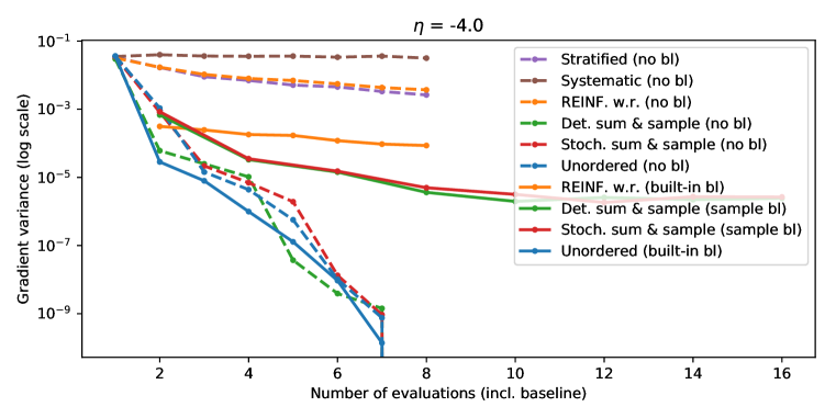
(b) Low entropy (Ξ·=βˆ’4πœ‚4\eta=-4)
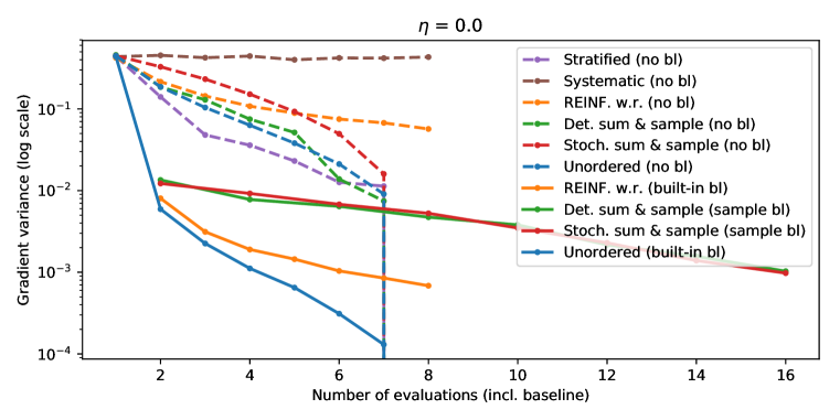
Figure 1: Bernoulli gradient variance (on log scale) as a function of the number of model evaluations (including baseline evaluations, so the sum-and-sample estimators with sampled baselines use twice as many evaluations). Note that for some estimators, the variance is 0 (log variance βˆ’βˆž-\infty) for k=8π‘˜8k=8.

We use the code by Liu etΒ al. (2019) to reproduce their Bernoulli toy experiment. Given a vector 𝐩=(0.6,0.51,0.48)𝐩0.60.510.48\mathbf{p}=(0.6,0.51,0.48) the goal is to minimize the loss ℒ​(Ξ·)=𝔼x1,x2,x3∼Bern​(σ​(Ξ·))​[βˆ‘i=13(xiβˆ’pi)2]β„’πœ‚subscript𝔼similar-tosubscriptπ‘₯1subscriptπ‘₯2subscriptπ‘₯3BernπœŽπœ‚delimited-[]superscriptsubscript𝑖13superscriptsubscriptπ‘₯𝑖subscript𝑝𝑖2\mathcal{L}(\eta)=\mathbb{E}_{x_{1},x_{2},x_{3}\sim\text{Bern}(\sigma(\eta))}\left[\sum_{i=1}^{3}(x_{i}-p_{i})^{2}\right]. Here x1,x2,x3subscriptπ‘₯1subscriptπ‘₯2subscriptπ‘₯3x_{1},x_{2},x_{3} are i.i.d. from the Bernoulli​(σ​(Ξ·))BernoulliπœŽπœ‚\text{Bernoulli}(\sigma(\eta)) distribution, parameterized by a scalar Ξ·βˆˆβ„πœ‚β„\eta\in\mathbb{R}, where σ​(Ξ·)=(1+exp⁑(βˆ’Ξ·))βˆ’1πœŽπœ‚superscript1πœ‚1\sigma(\eta)=(1+\exp(-\eta))^{-1} is the sigmoid function. We compare different estimators, with and without baseline (either β€˜built-in’ or using additional samples, referred to as REINFORCE+ in Liu etΒ al. (2019)). We report the (log-)variance of the scalar gradient βˆ‚β„’βˆ‚Ξ·β„’πœ‚\frac{\partial\mathcal{L}}{\partial\eta} as a function of the number of model evaluations, which is twice as high when using a sampled baseline (for each term).

As can be seen in Figure 1, the unordered set estimator is the only estimator that has consistently the lowest (or comparable) variance in both the high (Ξ·=0πœ‚0\eta=0) and low entropy (Ξ·=βˆ’4πœ‚4\eta=-4) regimes and for different number of samples/model evaluations. This suggests that it combines the advantages of the other estimators. We also ran the actual optimization experiment, where with as few as k=3π‘˜3k=3 samples the trajectory was indistinguishable from using the exact gradient (see Liu etΒ al. (2019)).

4.2 Categorical Variational Auto-Encoder

We use the code from Yin etΒ al. (2019) to train a categorical Variational Auto-Encoder (VAE) with 20 dimensional latent space, with 10 categories per dimension (details in Appendix G.1). To use our estimator, we treat this as a single factorized distribution with 1020superscript102010^{20} categories from which we can sample without replacement using Stochastic Beam Search (Kool etΒ al., 2019c), sequentially sampling each dimension as if it were a sequence model. We also perform experiments with 102superscript10210^{2} latent space, which provides a lower entropy setting, to highlight the advantage of our estimator.

Measuring the variance.
Table 1: VAE gradient log-variance of different unbiased estimators with k=4π‘˜4k=4 samples.
ARSM RELAX REINFORCE Sum & sample REINF. w.r. Unordered
Domain (no bl) (sample bl) (no bl) (sample bl) (built-in bl) (built-in bl)
Small 102superscript10210^{2} 13.45 11.67 11.52 7.49 6.29 6.29 6.65 6.29
Large 1020superscript102010^{20} 15.55 15.86 13.81 8.48 13.77 8.44 7.06 7.05

In Table 1, we report the variance of different gradient estimators with k=4π‘˜4k=4 samples, evaluated on a trained model. The unordered set estimator has the lowest variance in both the small and large domain (low and high entropy) setting, being on-par with the best of the (stochastic333We cannot use the deterministic version by Liu etΒ al. (2019) since we cannot select the top kπ‘˜k categories.) sum-and-sample estimator and REINFORCE with replacement444We cannot compare against VIMCO (Mnih & Rezende, 2016) as it optimizes a different objective.. This confirms the toy experiment, suggesting that the unordered set estimator provides the best of both estimators. In Appendix G.2 we repeat the same experiment at different stages of training, with similar results.
Refer to caption
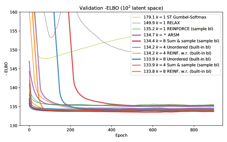
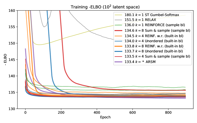
(a) Small domain (latent space size 102superscript10210^{2})
Refer to caption
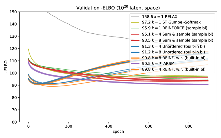
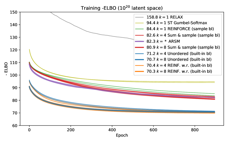
(b) Large domain (latent space size 1020superscript102010^{20})
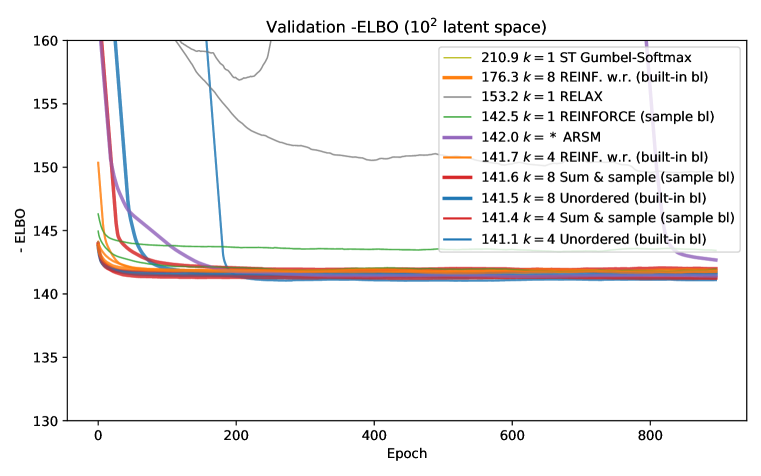
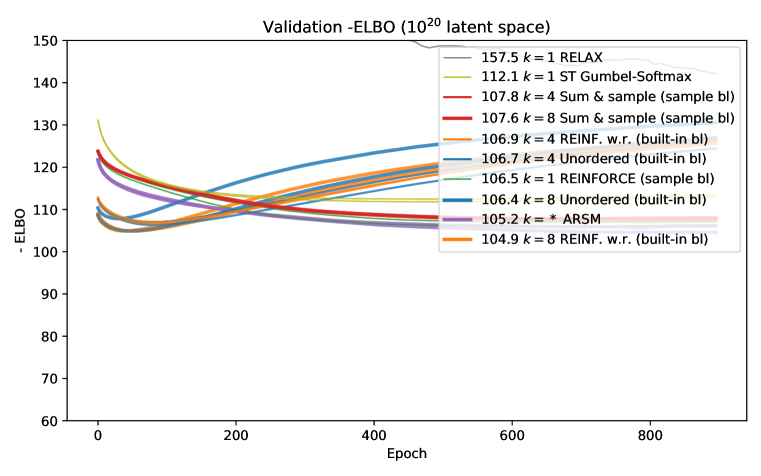
Figure 2: VAE smoothed training curves (-ELBO) of two independent runs when training with different estimators with k=1π‘˜1k=1, 4 or 8 (thicker lines) samples (ARSM has a variable number). Some lines coincide, so we sort the legend by the lowest -ELBO achieved and report this value.
ELBO optimization.

We use different estimators to optimize the ELBO (details in Appendix G.1). Additionally to the baselines by Yin etΒ al. (2019) we compare against REINFORCE with replacement and the stochastic sum-and-sample estimator. In Figure 2 we observe that our estimator performs on par with REINFORCE with replacement (and built-in baseline, equationΒ 23) and outperforms other estimators in at least one of the settings. There are a lot of other factors, e.g.Β exploration that may explain why we do not get a strictly better result despite the lower variance. We note some overfitting (see validation curves in Appendix G.2), but since our goal is to show improved optimization, and to keep results directly comparable to Yin etΒ al. (2019), we consider regularization a separate issue outside the scope of this paper. These results are using MNIST binarized by a threshold of 0.5. In Appendix G.2 we report results using the standard binarized MNIST dataset from Salakhutdinov & Murray (2008).

4.3 Structured Prediction for the Travelling Salesman Problem

To show the wide applicability of our estimator, we consider the structured prediction task of predicting routes (sequences) for the Travelling Salesman Problem (TSP) (Vinyals etΒ al., 2015; Bello etΒ al., 2016; Kool etΒ al., 2019a). We use the code by Kool etΒ al. (2019a)555https://github.com/wouterkool/attention-learn-to-route to reproduce their TSP experiment with 20 nodes. For details, see Appendix H.

We implement REINFORCE with replacement (and built-in baseline) as well as the stochastic sum-and-sample estimator and our estimator, using Stochastic Beam Search (Kool etΒ al., 2019c) for sampling. Also, we include results using the biased normalized importance-weighted policy gradient estimator with built-in baseline (derived in Kool etΒ al. (2019b), see Appendix D.2). Additionally, we compare against REINFORCE with greedy rollout baseline (Rennie etΒ al., 2017) used by Kool etΒ al. (2019c) and a batch-average baseline. For reference, we also include the biased risk estimator, either β€˜sampling’ using stochastic or deterministic beam search (as in Edunov etΒ al. (2018)).

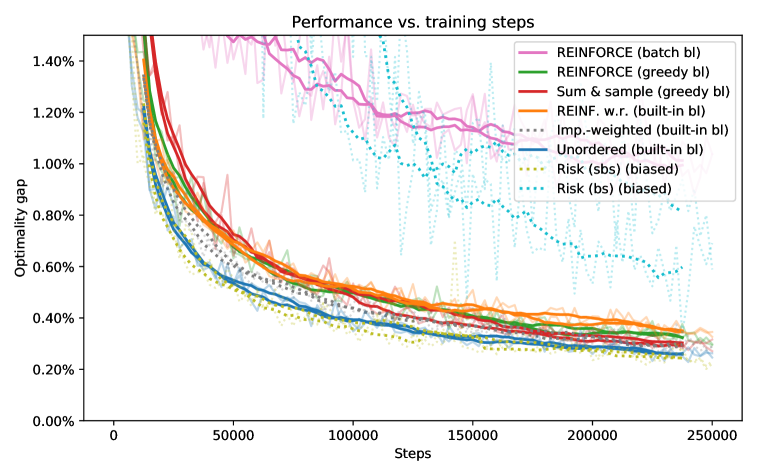
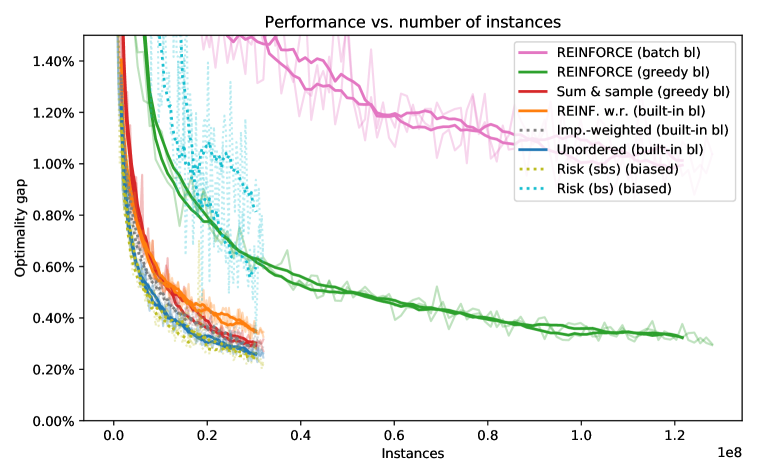
In Figure 3(a), we compare training progress (measured on the validation set) as a function of the number of training steps, where we divide the batch size by kπ‘˜k to keep the total number of samples equal. Our estimator outperforms REINFORCE with replacement, the stochastic sum-and-sample estimator and the strong greedy rollout baseline (which uses additional baseline model evaluations) and performs on-par with the biased risk estimator. In Figure 3(b), we plot the same results against the number of instances, which shows that, compared to the single sample estimators, we can train with less data and less computational cost (as we only need to run the encoder once for each instance).
Refer to caption
(a) Performance vs. training steps
Refer to caption
(b) Performance vs. number of instances
Figure 3: TSP validation set optimality gap measured during training. Raw results are light, smoothed results are darker (2 random seeds). We compare our estimator against different unbiased and biased (dotted) multi-sample estimators and against single-sample REINFORCE, with batch-average or greedy rollout baseline.

5 Discussion

We introduced the unordered set estimator, a low-variance, unbiased gradient estimator based on sampling without replacement, which can be used as an alternative to the popular biased Gumbel-Softmax estimator (Jang etΒ al., 2016; Maddison etΒ al., 2016). Our estimator is the result of Rao-Blackwellizing three existing estimators, which guarantees equal or lower variance, and is closely related to a number of other estimators. It has wide applicability, is parameter free (except for the sample size kπ‘˜k) and has competitive performance to the best of alternatives in both high and low entropy regimes.

In our experiments, we found that REINFORCE with replacement, with multiple samples and a built-in baseline as inspired by VIMCO (Mnih & Rezende, 2016), is a simple yet strong estimator which has performance similar to our estimator in the high entropy setting. We are not aware of any recent work on gradient estimators for discrete distributions that has considered this estimator as baseline, while it may be often preferred given its simplicity. In future work, we want to investigate if we can apply our estimator to estimate gradients β€˜locally’ (Titsias & LΓ‘zaro-Gredilla, 2015), as locally we have a smaller domain and expect more duplicate samples.

Acknowledgments

This research was funded by ORTEC. We would like to thank anonymous reviewers for their feedback that helped improve the paper.

References

  • Bahdanau etΒ al. (2017) Dzmitry Bahdanau, Philemon Brakel, Kelvin Xu, Anirudh Goyal, Ryan Lowe, Joelle Pineau, Aaron Courville, and Yoshua Bengio. An actor-critic algorithm for sequence prediction. In International Conference on Learning Representations, 2017.
  • Bello etΒ al. (2016) Irwan Bello, Hieu Pham, QuocΒ V Le, Mohammad Norouzi, and Samy Bengio. Neural combinatorial optimization with reinforcement learning. arXiv preprint arXiv:1611.09940, 2016.
  • Bengio etΒ al. (2013) Yoshua Bengio, Nicholas LΓ©onard, and Aaron Courville. Estimating or propagating gradients through stochastic neurons for conditional computation. arXiv preprint arXiv:1308.3432, 2013.
  • Casella & Robert (1996) George Casella and ChristianΒ P Robert. Rao-Blackwellisation of sampling schemes. Biometrika, 83(1):81–94, 1996.
  • Douc & CappΓ© (2005) Randal Douc and Olivier CappΓ©. Comparison of resampling schemes for particle filtering. In ISPA 2005. Proceedings of the 4th International Symposium on Image and Signal Processing and Analysis, 2005., pp.Β  64–69. IEEE, 2005.
  • Duffield etΒ al. (2007) Nick Duffield, Carsten Lund, and Mikkel Thorup. Priority sampling for estimation of arbitrary subset sums. Journal of the ACM (JACM), 54(6):32, 2007.
  • Edunov etΒ al. (2018) Sergey Edunov, Myle Ott, Michael Auli, David Grangier, etΒ al. Classical structured prediction losses for sequence to sequence learning. In Proceedings of the 2018 Conference of the North American Chapter of the Association for Computational Linguistics: Human Language Technologies, Volume 1 (Long Papers), volumeΒ 1, pp.Β  355–364, 2018.
  • Fearnhead & Clifford (2003) Paul Fearnhead and Peter Clifford. On-line inference for hidden markov models via particle filters. Journal of the Royal Statistical Society: Series B (Statistical Methodology), 65(4):887–899, 2003.
  • Grathwohl etΒ al. (2018) Will Grathwohl, Dami Choi, Yuhuai Wu, Geoffrey Roeder, and David Duvenaud. Backpropagation through the void: Optimizing control variates for black-box gradient estimation. In International Conference on Learning Representations, 2018.
  • Gregor etΒ al. (2014) Karol Gregor, Ivo Danihelka, Andriy Mnih, Charles Blundell, and Daan Wierstra. Deep autoregressive networks. In International Conference on Machine Learning, pp.Β 1242–1250, 2014.
  • Grover etΒ al. (2019) Aditya Grover, Eric Wang, Aaron Zweig, and Stefano Ermon. Stochastic optimization of sorting networks via continuous relaxations. In International Conference on Learning Representations, 2019.
  • Gu etΒ al. (2018) Jiatao Gu, DanielΒ Jiwoong Im, and VictorΒ OK Li. Neural machine translation with Gumbel-greedy decoding. In Thirty-Second AAAI Conference on Artificial Intelligence (AAAI), 2018.
  • Gu etΒ al. (2016) Shixiang Gu, Sergey Levine, Ilya Sutskever, and Andriy Mnih. Muprop: Unbiased backpropagation for stochastic neural networks. In International Conference on Learning Representations, 2016.
  • He etΒ al. (2016) DiΒ He, Yingce Xia, Tao Qin, Liwei Wang, Nenghai Yu, Tie-Yan Liu, and Wei-Ying Ma. Dual learning for machine translation. In Advances in Neural Information Processing Systems, pp.Β 820–828, 2016.
  • Jang etΒ al. (2016) Eric Jang, Shixiang Gu, and Ben Poole. Categorical reparameterization with gumbel-softmax. In International Conference on Learning Representations, 2016.
  • Kim etΒ al. (2016) Carolyn Kim, Ashish Sabharwal, and Stefano Ermon. Exact sampling with integer linear programs and random perturbations. In Thirtieth AAAI Conference on Artificial Intelligence, 2016.
  • Kingma & Ba (2015) DiederikΒ P Kingma and Jimmy Ba. Adam: A method for stochastic optimization. In International Conference on Learning Representations, 2015.
  • Kingma & Welling (2014) DiederikΒ P Kingma and Max Welling. Auto-encoding variational Bayes. In International Conference on Learning Representations, 2014.
  • Kool etΒ al. (2019a) Wouter Kool, Herke van Hoof, and Max Welling. Attention, learn to solve routing problems! In International Conference on Learning Representations, 2019a.
  • Kool etΒ al. (2019b) Wouter Kool, Herke van Hoof, and Max Welling. Buy 4 reinforce samples, get a baseline for free! In Deep Reinforcement Learning Meets Structured Prediction Workshop at the International Conference on Learning Representations, 2019b.
  • Kool etΒ al. (2019c) Wouter Kool, Herke VanΒ Hoof, and Max Welling. Stochastic beams and where to find them: The gumbel-top-k trick for sampling sequences without replacement. In International Conference on Machine Learning, pp.Β 3499–3508, 2019c.
  • Larochelle & Murray (2011) Hugo Larochelle and Iain Murray. The neural autoregressive distribution estimator. In Proceedings of the Fourteenth International Conference on Artificial Intelligence and Statistics, pp.Β  29–37, 2011.
  • Leblond etΒ al. (2018) RΓ©mi Leblond, Jean-Baptiste Alayrac, Anton Osokin, and Simon Lacoste-Julien. Searnn: Training RNNs with global-local losses. In 6th International Conference on Learning Representations, 2018.
  • Lehmann & ScheffΓ© (1950) ELΒ Lehmann and Henry ScheffΓ©. Completeness, similar regions, and unbiased estimation: Part i. Sankhyā: The Indian Journal of Statistics, pp.Β  305–340, 1950.
  • Liang etΒ al. (2018) Chen Liang, Mohammad Norouzi, Jonathan Berant, QuocΒ V Le, and NiΒ Lao. Memory augmented policy optimization for program synthesis and semantic parsing. In Advances in Neural Information Processing Systems, pp.Β 9994–10006, 2018.
  • Liu etΒ al. (2019) Runjing Liu, Jeffrey Regier, Nilesh Tripuraneni, Michael Jordan, and Jon Mcauliffe. Rao-Blackwellized stochastic gradients for discrete distributions. In International Conference on Machine Learning, pp.Β 4023–4031, 2019.
  • Lorberbom etΒ al. (2018) Guy Lorberbom, Andreea Gane, Tommi Jaakkola, and Tamir Hazan. Direct optimization through argmax for discrete variational auto-encoder. arXiv preprint arXiv:1806.02867, 2018.
  • Lorberbom etΒ al. (2019) Guy Lorberbom, ChrisΒ J Maddison, Nicolas Heess, Tamir Hazan, and Daniel Tarlow. Direct policy gradients: Direct optimization of policies in discrete action spaces. arXiv preprint arXiv:1906.06062, 2019.
  • Luce (1959) RΒ Duncan Luce. Individual choice behavior: A theoretical analysis. John Wiley, 1959.
  • Maddison etΒ al. (2014) ChrisΒ J Maddison, Daniel Tarlow, and Tom Minka. A* sampling. In Advances in Neural Information Processing Systems, pp.Β 3086–3094, 2014.
  • Maddison etΒ al. (2016) ChrisΒ J Maddison, Andriy Mnih, and YeeΒ Whye Teh. The concrete distribution: A continuous relaxation of discrete random variables. In International Conference on Learning Representations, 2016.
  • Mnih & Gregor (2014) Andriy Mnih and Karol Gregor. Neural variational inference and learning in belief networks. In International Conference on Machine Learning, pp.Β 1791–1799, 2014.
  • Mnih & Rezende (2016) Andriy Mnih and Danilo Rezende. Variational inference for Monte Carlo objectives. In International Conference on Machine Learning, pp.Β 2188–2196, 2016.
  • Murthy (1957) MNΒ Murthy. Ordered and unordered estimators in sampling without replacement. Sankhyā: The Indian Journal of Statistics (1933-1960), 18(3/4):379–390, 1957.
  • Negrinho etΒ al. (2018) Renato Negrinho, Matthew Gormley, and GeoffreyΒ J Gordon. Learning beam search policies via imitation learning. In Advances in Neural Information Processing Systems, pp.Β 10673–10682, 2018.
  • Norouzi etΒ al. (2016) Mohammad Norouzi, Samy Bengio, Navdeep Jaitly, Mike Schuster, Yonghui Wu, Dale Schuurmans, etΒ al. Reward augmented maximum likelihood for neural structured prediction. In Advances In Neural Information Processing Systems, pp.Β 1723–1731, 2016.
  • Paisley etΒ al. (2012) John Paisley, DavidΒ M Blei, and MichaelΒ I Jordan. Variational Bayesian inference with stochastic search. In International Conference on Machine Learning, pp.Β 1363–1370, 2012.
  • Plackett (1975) RobinΒ L Plackett. The analysis of permutations. Journal of the Royal Statistical Society: Series C (Applied Statistics), 24(2):193–202, 1975.
  • Raj (1956) Des Raj. Some estimators in sampling with varying probabilities without replacement. Journal of the American Statistical Association, 51(274):269–284, 1956.
  • Ranganath etΒ al. (2014) Rajesh Ranganath, Sean Gerrish, and David Blei. Black box variational inference. In Artificial Intelligence and Statistics, pp.Β  814–822, 2014.
  • Ranzato etΒ al. (2016) Marc’Aurelio Ranzato, Sumit Chopra, Michael Auli, and Wojciech Zaremba. Sequence level training with recurrent neural networks. In International Conference on Learning Representations, 2016.
  • Rennie etΒ al. (2017) StevenΒ J Rennie, Etienne Marcheret, Youssef Mroueh, Jerret Ross, and Vaibhava Goel. Self-critical sequence training for image captioning. In Proceedings of the IEEE Conference on Computer Vision and Pattern Recognition, pp.Β  7008–7024, 2017.
  • Rezende etΒ al. (2014) DaniloΒ Jimenez Rezende, Shakir Mohamed, and Daan Wierstra. Stochastic backpropagation and approximate inference in deep generative models. In International Conference on Machine Learning, pp.Β 1278–1286, 2014.
  • Roeder etΒ al. (2017) Geoffrey Roeder, Yuhuai Wu, and DavidΒ K Duvenaud. Sticking the landing: Simple, lower-variance gradient estimators for variational inference. In Advances in Neural Information Processing Systems, pp.Β 6925–6934, 2017.
  • Salakhutdinov & Murray (2008) Ruslan Salakhutdinov and Iain Murray. On the quantitative analysis of deep belief networks. In International Conference on Machine Learning, pp.Β 872–879, 2008.
  • Schulman etΒ al. (2015) John Schulman, Nicolas Heess, Theophane Weber, and Pieter Abbeel. Gradient estimation using stochastic computation graphs. In Advances in Neural Information Processing Systems, pp.Β 3528–3536, 2015.
  • Shen etΒ al. (2016) Shiqi Shen, Yong Cheng, Zhongjun He, Wei He, Hua Wu, Maosong Sun, and Yang Liu. Minimum risk training for neural machine translation. In Proceedings of the 54th Annual Meeting of the Association for Computational Linguistics (Volume 1: Long Papers), volumeΒ 1, pp.Β 1683–1692, 2016.
  • Sutton & Barto (2018) RichardΒ S Sutton and AndrewΒ G Barto. Reinforcement learning: An introduction. MIT press, 2018.
  • Titsias & LΓ‘zaro-Gredilla (2015) MichalisΒ K Titsias and Miguel LΓ‘zaro-Gredilla. Local expectation gradients for black box variational inference. In Advances in Neural Information Processing Systems-Volume 2, pp.Β  2638–2646, 2015.
  • Tucker etΒ al. (2017) George Tucker, Andriy Mnih, ChrisΒ J Maddison, John Lawson, and Jascha Sohl-Dickstein. Rebar: Low-variance, unbiased gradient estimates for discrete latent variable models. In Advances in Neural Information Processing Systems, pp.Β 2627–2636, 2017.
  • Vieira (2014) Tim Vieira. Gumbel-max trick and weighted reservoir sampling, 2014. URL https://timvieira.github.io/blog/post/2014/08/01/gumbel-max-trick-and-weighted-reservoir-sampling/.
  • Vieira (2017) Tim Vieira. Estimating means in a finite universe, 2017. URL https://timvieira.github.io/blog/post/2017/07/03/estimating-means-in-a-finite-universe/.
  • Vinyals etΒ al. (2015) Oriol Vinyals, Meire Fortunato, and Navdeep Jaitly. Pointer networks. In Advances in Neural Information Processing Systems, pp.Β 2692–2700, 2015.
  • Williams (1992) RonaldΒ J Williams. Simple statistical gradient-following algorithms for connectionist reinforcement learning. Machine learning, 8(3-4):229–256, 1992.
  • Yellott (1977) JohnΒ I Yellott. The relationship between Luce’s choice axiom, Thurstone’s theory of comparative judgment, and the double exponential distribution. Journal of Mathematical Psychology, 15(2):109–144, 1977.
  • Yin etΒ al. (2019) Mingzhang Yin, Yuguang Yue, and Mingyuan Zhou. Arsm: Augment-reinforce-swap-merge estimator for gradient backpropagation through categorical variables. In International Conference on Machine Learning, pp.Β 7095–7104, 2019.

Appendix A Notation

Throughout this appendix we will use the following notation from Maddison etΒ al. (2014):

eϕ​(g)subscript𝑒italic-ϕ𝑔\displaystyle e_{\phi}(g) =exp⁑(βˆ’g+Ο•)absent𝑔italic-Ο•\displaystyle=\exp(-g+\phi)
Fϕ​(g)subscript𝐹italic-ϕ𝑔\displaystyle F_{\phi}(g) =exp⁑(βˆ’exp⁑(βˆ’g+Ο•))absent𝑔italic-Ο•\displaystyle=\exp(-\exp(-g+\phi))
fϕ​(g)subscript𝑓italic-ϕ𝑔\displaystyle f_{\phi}(g) =eϕ​(g)​Fϕ​(g).absentsubscript𝑒italic-ϕ𝑔subscript𝐹italic-ϕ𝑔\displaystyle=e_{\phi}(g)F_{\phi}(g).

This means that Fϕ​(g)subscript𝐹italic-ϕ𝑔F_{\phi}(g) is the CDF and fϕ​(g)subscript𝑓italic-ϕ𝑔f_{\phi}(g) the PDF of the Gumbel​(Ο•)Gumbelitalic-Ο•\text{Gumbel}(\phi) distribution. Additionally we will use the identities by Maddison etΒ al. (2014):

Fϕ​(g)​Fγ​(g)subscript𝐹italic-ϕ𝑔subscript𝐹𝛾𝑔\displaystyle F_{\phi}(g)F_{\gamma}(g) =Flog⁑(exp⁑(Ο•)+exp⁑(Ξ³))​(g)absentsubscript𝐹italic-ϕ𝛾𝑔\displaystyle=F_{\log(\exp(\phi)+\exp(\gamma))}(g) (24)
∫g=abeγ​(g)​Fϕ​(g)β€‹βˆ‚gsuperscriptsubscriptπ‘”π‘Žπ‘subscript𝑒𝛾𝑔subscript𝐹italic-ϕ𝑔𝑔\displaystyle\int_{g=a}^{b}e_{\gamma}(g)F_{\phi}(g)\partial g =(Fϕ​(b)βˆ’Fϕ​(a))​exp⁑(Ξ³)exp⁑(Ο•).absentsubscript𝐹italic-ϕ𝑏subscript𝐹italic-Ο•π‘Žπ›Ύitalic-Ο•\displaystyle=(F_{\phi}(b)-F_{\phi}(a))\frac{\exp(\gamma)}{\exp(\phi)}. (25)

Also, we will use the following notation, definitions and identities (see Kool etΒ al. (2019c)):

Ο•isubscriptitalic-ϕ𝑖\displaystyle\phi_{i} =log⁑p​(i)absent𝑝𝑖\displaystyle=\log p(i) (26)
Ο•Ssubscriptitalic-ϕ𝑆\displaystyle\phi_{S} =logβ€‹βˆ‘i∈Sp​(i)=logβ€‹βˆ‘i∈Sexp⁑ϕiabsentsubscript𝑖𝑆𝑝𝑖subscript𝑖𝑆subscriptitalic-ϕ𝑖\displaystyle=\log\sum_{i\in S}p(i)=\log\sum_{i\in S}\exp\phi_{i} (27)
Ο•Dβˆ–Ssubscriptitalic-ϕ𝐷𝑆\displaystyle\phi_{D\setminus S} =logβ€‹βˆ‘i∈Dβˆ–Sp​(i)=log⁑(1βˆ’βˆ‘i∈Sp​(i))=log⁑(1βˆ’exp⁑(Ο•S))absentsubscript𝑖𝐷𝑆𝑝𝑖1subscript𝑖𝑆𝑝𝑖1subscriptitalic-ϕ𝑆\displaystyle=\log\sum_{i\in D\setminus S}p(i)=\log\left(1-\sum_{i\in S}p(i)\right)=\log(1-\exp(\phi_{S})) (28)
GΟ•isubscript𝐺subscriptitalic-ϕ𝑖\displaystyle G_{\phi_{i}} ∼Gumbel​(Ο•i)similar-toabsentGumbelsubscriptitalic-ϕ𝑖\displaystyle\sim\text{Gumbel}(\phi_{i}) (29)
GΟ•Ssubscript𝐺subscriptitalic-ϕ𝑆\displaystyle G_{\phi_{S}} =maxi∈S⁑GΟ•i∼Gumbel​(Ο•S)absentsubscript𝑖𝑆subscript𝐺subscriptitalic-ϕ𝑖similar-toGumbelsubscriptitalic-ϕ𝑆\displaystyle=\max_{i\in S}G_{\phi_{i}}\sim\text{Gumbel}(\phi_{S}) (30)

For a proof of equationΒ 30, see Maddison etΒ al. (2014).

Appendix B Computation of p​(Sk)𝑝superscriptπ‘†π‘˜p(S^{k}), pDβˆ–C​(Sβˆ–C)superscript𝑝𝐷𝐢𝑆𝐢p^{D\setminus C}(S\setminus C) and R​(Sk,s)𝑅superscriptπ‘†π‘˜π‘ R(S^{k},s)

We can sample the set Sksuperscriptπ‘†π‘˜S^{k} from the Plackett-Luce distribution using the Gumbel-Top-kπ‘˜k trick by drawing Gumbel variables GΟ•i∼Gumbel​(Ο•i)similar-tosubscript𝐺subscriptitalic-ϕ𝑖Gumbelsubscriptitalic-ϕ𝑖G_{\phi_{i}}\sim\text{Gumbel}(\phi_{i}) for each element and returning the indices of the kπ‘˜k largest Gumbels. If we ignore the ordering, this means we will obtain the set Sksuperscriptπ‘†π‘˜S^{k} if mini∈Sk⁑GΟ•i>maxi∈Dβˆ–Sk⁑GΟ•isubscript𝑖superscriptπ‘†π‘˜subscript𝐺subscriptitalic-ϕ𝑖subscript𝑖𝐷superscriptπ‘†π‘˜subscript𝐺subscriptitalic-ϕ𝑖\min_{i\in S^{k}}G_{\phi_{i}}>\max_{i\in D\setminus S^{k}}G_{\phi_{i}}. Omitting the superscript kπ‘˜k for clarity, we can use the Gumbel-Max trick, i.e.Β that GΟ•Dβˆ–S=maxiβˆ‰S⁑GΟ•i∼Gumbel​(Ο•Dβˆ–S)subscript𝐺subscriptitalic-ϕ𝐷𝑆subscript𝑖𝑆subscript𝐺subscriptitalic-ϕ𝑖similar-toGumbelsubscriptitalic-ϕ𝐷𝑆G_{\phi_{D\setminus S}}=\max_{i\not\in S}G_{\phi_{i}}\sim\text{Gumbel}(\phi_{D\setminus S}) (equationΒ 30) and marginalize over GΟ•Dβˆ–Ssubscript𝐺subscriptitalic-ϕ𝐷𝑆G_{\phi_{D\setminus S}}:

p​(S)𝑝𝑆\displaystyle p(S) =P​(mini∈S⁑GΟ•i>GΟ•Dβˆ–S)absent𝑃subscript𝑖𝑆subscript𝐺subscriptitalic-ϕ𝑖subscript𝐺subscriptitalic-ϕ𝐷𝑆\displaystyle=P(\min_{i\in S}G_{\phi_{i}}>G_{\phi_{D\setminus S}})
=P​(GΟ•i>GΟ•Dβˆ–S,i∈S)absent𝑃formulae-sequencesubscript𝐺subscriptitalic-ϕ𝑖subscript𝐺subscriptitalic-ϕ𝐷𝑆𝑖𝑆\displaystyle=P(G_{\phi_{i}}>G_{\phi_{D\setminus S}},i\in S)
=∫gΟ•Dβˆ–S=βˆ’βˆžβˆžfΟ•Dβˆ–S​(gΟ•Dβˆ–S)​P​(GΟ•i>gΟ•Dβˆ–S,i∈S)β€‹βˆ‚gΟ•Dβˆ–Sabsentsuperscriptsubscriptsubscript𝑔subscriptitalic-ϕ𝐷𝑆subscript𝑓subscriptitalic-ϕ𝐷𝑆subscript𝑔subscriptitalic-ϕ𝐷𝑆𝑃formulae-sequencesubscript𝐺subscriptitalic-ϕ𝑖subscript𝑔subscriptitalic-ϕ𝐷𝑆𝑖𝑆subscript𝑔subscriptitalic-ϕ𝐷𝑆\displaystyle=\int_{g_{\phi_{D\setminus S}}=-\infty}^{\infty}f_{\phi_{D\setminus S}}(g_{\phi_{D\setminus S}})P(G_{\phi_{i}}>g_{\phi_{D\setminus S}},i\in S)\partial g_{\phi_{D\setminus S}}
=∫gΟ•Dβˆ–S=βˆ’βˆžβˆžfΟ•Dβˆ–S​(gΟ•Dβˆ–S)β€‹βˆi∈S(1βˆ’FΟ•i​(gΟ•Dβˆ–S))β€‹βˆ‚gΟ•Dβˆ–Sabsentsuperscriptsubscriptsubscript𝑔subscriptitalic-ϕ𝐷𝑆subscript𝑓subscriptitalic-ϕ𝐷𝑆subscript𝑔subscriptitalic-ϕ𝐷𝑆subscriptproduct𝑖𝑆1subscript𝐹subscriptitalic-ϕ𝑖subscript𝑔subscriptitalic-ϕ𝐷𝑆subscript𝑔subscriptitalic-ϕ𝐷𝑆\displaystyle=\int_{g_{\phi_{D\setminus S}}=-\infty}^{\infty}f_{\phi_{D\setminus S}}(g_{\phi_{D\setminus S}})\prod_{i\in S}\left(1-F_{\phi_{i}}(g_{\phi_{D\setminus S}})\right)\partial g_{\phi_{D\setminus S}} (31)
=∫u=01∏i∈S(1βˆ’FΟ•i​(FΟ•Dβˆ–Sβˆ’1​(u)))β€‹βˆ‚uabsentsuperscriptsubscript𝑒01subscriptproduct𝑖𝑆1subscript𝐹subscriptitalic-ϕ𝑖subscriptsuperscript𝐹1subscriptitalic-ϕ𝐷𝑆𝑒𝑒\displaystyle=\int_{u=0}^{1}\prod_{i\in S}\left(1-F_{\phi_{i}}\left(F^{-1}_{\phi_{D\setminus S}}(u)\right)\right)\partial u (32)

Here we have used a change of variables u=FΟ•Dβˆ–S​(gΟ•Dβˆ–S)𝑒subscript𝐹subscriptitalic-ϕ𝐷𝑆subscript𝑔subscriptitalic-ϕ𝐷𝑆u=F_{\phi_{D\setminus S}}(g_{\phi_{D\setminus S}}). This expression can be efficiently numerically integrated (although another change of variables may be required for numerical stability depending on the values of Ο•bold-italic-Ο•\bm{\phi}).

Exact computation in O​(2k)𝑂superscript2π‘˜O(2^{k}).

The integral in equationΒ 31 can be computed exactly using the identity

∏i∈S(aiβˆ’bi)=βˆ‘CβŠ†S(βˆ’1)|C|β€‹βˆi∈Cbiβ€‹βˆi∈Sβˆ–Caisubscriptproduct𝑖𝑆subscriptπ‘Žπ‘–subscript𝑏𝑖subscript𝐢𝑆superscript1𝐢subscriptproduct𝑖𝐢subscript𝑏𝑖subscriptproduct𝑖𝑆𝐢subscriptπ‘Žπ‘–\prod_{i\in S}(a_{i}-b_{i})=\sum_{C\subseteq S}(-1)^{|C|}\prod_{i\in C}b_{i}\prod_{i\in S\setminus C}a_{i}

which gives

p​(S)𝑝𝑆\displaystyle p(S) =∫gΟ•Dβˆ–S=βˆ’βˆžβˆžfΟ•Dβˆ–S​(gΟ•Dβˆ–S)β€‹βˆi∈S(1βˆ’FΟ•i​(gΟ•Dβˆ–S))β€‹βˆ‚gΟ•Dβˆ–Sabsentsuperscriptsubscriptsubscript𝑔subscriptitalic-ϕ𝐷𝑆subscript𝑓subscriptitalic-ϕ𝐷𝑆subscript𝑔subscriptitalic-ϕ𝐷𝑆subscriptproduct𝑖𝑆1subscript𝐹subscriptitalic-ϕ𝑖subscript𝑔subscriptitalic-ϕ𝐷𝑆subscript𝑔subscriptitalic-ϕ𝐷𝑆\displaystyle=\int_{g_{\phi_{D\setminus S}}=-\infty}^{\infty}f_{\phi_{D\setminus S}}(g_{\phi_{D\setminus S}})\prod_{i\in S}\left(1-F_{\phi_{i}}(g_{\phi_{D\setminus S}})\right)\partial g_{\phi_{D\setminus S}}
=βˆ‘CβŠ†S(βˆ’1)|C|β€‹βˆ«gΟ•Dβˆ–S=βˆ’βˆžβˆžfΟ•Dβˆ–S​(gΟ•Dβˆ–S)β€‹βˆi∈CFΟ•i​(gΟ•Dβˆ–S)β€‹βˆi∈Sβˆ–C1β€‹βˆ‚gΟ•Dβˆ–Sabsentsubscript𝐢𝑆superscript1𝐢superscriptsubscriptsubscript𝑔subscriptitalic-ϕ𝐷𝑆subscript𝑓subscriptitalic-ϕ𝐷𝑆subscript𝑔subscriptitalic-ϕ𝐷𝑆subscriptproduct𝑖𝐢subscript𝐹subscriptitalic-ϕ𝑖subscript𝑔subscriptitalic-ϕ𝐷𝑆subscriptproduct𝑖𝑆𝐢1subscript𝑔subscriptitalic-ϕ𝐷𝑆\displaystyle=\sum_{C\subseteq S}(-1)^{|C|}\int_{g_{\phi_{D\setminus S}}=-\infty}^{\infty}f_{\phi_{D\setminus S}}(g_{\phi_{D\setminus S}})\prod_{i\in C}F_{\phi_{i}}(g_{\phi_{D\setminus S}})\prod_{i\in S\setminus C}1\partial g_{\phi_{D\setminus S}}
=βˆ‘CβŠ†S(βˆ’1)|C|β€‹βˆ«gΟ•Dβˆ–S=βˆ’βˆžβˆžeΟ•Dβˆ–S​(gΟ•Dβˆ–S)​FΟ•Dβˆ–S​(gΟ•Dβˆ–S)​FΟ•C​(gΟ•Dβˆ–S)β€‹βˆ‚gΟ•Dβˆ–Sabsentsubscript𝐢𝑆superscript1𝐢superscriptsubscriptsubscript𝑔subscriptitalic-ϕ𝐷𝑆subscript𝑒subscriptitalic-ϕ𝐷𝑆subscript𝑔subscriptitalic-ϕ𝐷𝑆subscript𝐹subscriptitalic-ϕ𝐷𝑆subscript𝑔subscriptitalic-ϕ𝐷𝑆subscript𝐹subscriptitalic-ϕ𝐢subscript𝑔subscriptitalic-ϕ𝐷𝑆subscript𝑔subscriptitalic-ϕ𝐷𝑆\displaystyle=\sum_{C\subseteq S}(-1)^{|C|}\int_{g_{\phi_{D\setminus S}}=-\infty}^{\infty}e_{\phi_{D\setminus S}}(g_{\phi_{D\setminus S}})F_{\phi_{D\setminus S}}(g_{\phi_{D\setminus S}})F_{\phi_{C}}(g_{\phi_{D\setminus S}})\partial g_{\phi_{D\setminus S}}
=βˆ‘CβŠ†S(βˆ’1)|C|β€‹βˆ«gΟ•Dβˆ–S=βˆ’βˆžβˆžeΟ•Dβˆ–S​(gΟ•Dβˆ–S)​FΟ•(Dβˆ–S)βˆͺC​(gΟ•Dβˆ–S)β€‹βˆ‚gΟ•Dβˆ–Sabsentsubscript𝐢𝑆superscript1𝐢superscriptsubscriptsubscript𝑔subscriptitalic-ϕ𝐷𝑆subscript𝑒subscriptitalic-ϕ𝐷𝑆subscript𝑔subscriptitalic-ϕ𝐷𝑆subscript𝐹subscriptitalic-ϕ𝐷𝑆𝐢subscript𝑔subscriptitalic-ϕ𝐷𝑆subscript𝑔subscriptitalic-ϕ𝐷𝑆\displaystyle=\sum_{C\subseteq S}(-1)^{|C|}\int_{g_{\phi_{D\setminus S}}=-\infty}^{\infty}e_{\phi_{D\setminus S}}(g_{\phi_{D\setminus S}})F_{\phi_{(D\setminus S)\cup C}}(g_{\phi_{D\setminus S}})\partial g_{\phi_{D\setminus S}}
=βˆ‘CβŠ†S(βˆ’1)|C|​(1βˆ’0)​exp⁑(Ο•Dβˆ–S)exp⁑(Ο•(Dβˆ–S)βˆͺC)absentsubscript𝐢𝑆superscript1𝐢10subscriptitalic-ϕ𝐷𝑆subscriptitalic-ϕ𝐷𝑆𝐢\displaystyle=\sum_{C\subseteq S}(-1)^{|C|}(1-0)\frac{\exp(\phi_{D\setminus S})}{\exp(\phi_{(D\setminus S)\cup C})}
=βˆ‘CβŠ†S(βˆ’1)|C|​1βˆ’βˆ‘i∈Sp​(i)1βˆ’βˆ‘i∈Sβˆ–Cp​(i).absentsubscript𝐢𝑆superscript1𝐢1subscript𝑖𝑆𝑝𝑖1subscript𝑖𝑆𝐢𝑝𝑖\displaystyle=\sum_{C\subseteq S}(-1)^{|C|}\frac{1-\sum_{i\in S}p(i)}{1-\sum_{i\in S\setminus C}p(i)}. (33)
Computation of pDβˆ–C​(Sβˆ–C)superscript𝑝𝐷𝐢𝑆𝐢p^{D\setminus C}(S\setminus C).

When using the Gumbel-Top-kπ‘˜k trick over the restricted domain Dβˆ–C𝐷𝐢D\setminus C, we do not need to renormalize the log-probabilities Ο•s,s∈Dβˆ–Csubscriptitalic-ϕ𝑠𝑠𝐷𝐢\phi_{s},s\in D\setminus C since the Gumbel-Top-kπ‘˜k trick applies to unnormalized log-probabilities. Also, assuming CβŠ†Sk𝐢superscriptπ‘†π‘˜C\subseteq S^{k}, it holds that (Dβˆ–C)βˆ–(Sβˆ–C)=Dβˆ–S𝐷𝐢𝑆𝐢𝐷𝑆(D\setminus C)\setminus(S\setminus C)=D\setminus S. This means that we can compute pDβˆ–C​(Sβˆ–C)superscript𝑝𝐷𝐢𝑆𝐢p^{D\setminus C}(S\setminus C) similar to equationΒ 31:

pDβˆ–C​(Sβˆ–C)superscript𝑝𝐷𝐢𝑆𝐢\displaystyle p^{D\setminus C}(S\setminus C) =P​(mini∈Sβˆ–C⁑GΟ•i>GΟ•(Dβˆ–C)βˆ–(Sβˆ–C))absent𝑃subscript𝑖𝑆𝐢subscript𝐺subscriptitalic-ϕ𝑖subscript𝐺subscriptitalic-ϕ𝐷𝐢𝑆𝐢\displaystyle=P(\min_{i\in S\setminus C}G_{\phi_{i}}>G_{\phi_{(D\setminus C)\setminus(S\setminus C)}})
=P​(mini∈Sβˆ–C⁑GΟ•i>GΟ•Dβˆ–S)absent𝑃subscript𝑖𝑆𝐢subscript𝐺subscriptitalic-ϕ𝑖subscript𝐺subscriptitalic-ϕ𝐷𝑆\displaystyle=P(\min_{i\in S\setminus C}G_{\phi_{i}}>G_{\phi_{D\setminus S}})
=∫gΟ•Dβˆ–S=βˆ’βˆžβˆžfΟ•Dβˆ–S​(gΟ•Dβˆ–S)β€‹βˆi∈Sβˆ–C(1βˆ’FΟ•i​(gΟ•Dβˆ–S))β€‹βˆ‚gΟ•Dβˆ–S.absentsuperscriptsubscriptsubscript𝑔subscriptitalic-ϕ𝐷𝑆subscript𝑓subscriptitalic-ϕ𝐷𝑆subscript𝑔subscriptitalic-ϕ𝐷𝑆subscriptproduct𝑖𝑆𝐢1subscript𝐹subscriptitalic-ϕ𝑖subscript𝑔subscriptitalic-ϕ𝐷𝑆subscript𝑔subscriptitalic-ϕ𝐷𝑆\displaystyle=\int_{g_{\phi_{D\setminus S}}=-\infty}^{\infty}f_{\phi_{D\setminus S}}(g_{\phi_{D\setminus S}})\prod_{i\in S\setminus C}\left(1-F_{\phi_{i}}(g_{\phi_{D\setminus S}})\right)\partial g_{\phi_{D\setminus S}}. (34)
Computation of R​(Sk,s)𝑅superscriptπ‘†π‘˜π‘ R(S^{k},s).

Note that, using equationΒ 10, it holds that

βˆ‘s∈SkpDβˆ–{s}​(Skβˆ–{s})​p​(s)p​(Sk)=βˆ‘s∈SkP​(b1=s|Sk)=1subscript𝑠superscriptπ‘†π‘˜superscript𝑝𝐷𝑠superscriptπ‘†π‘˜π‘ π‘π‘ π‘superscriptπ‘†π‘˜subscript𝑠superscriptπ‘†π‘˜π‘ƒsubscript𝑏1conditional𝑠superscriptπ‘†π‘˜1\sum_{s\in S^{k}}\frac{p^{D\setminus\{s\}}(S^{k}\setminus\{s\})p(s)}{p(S^{k})}=\sum_{s\in S^{k}}P(b_{1}=s|S^{k})=1

from which it follows that

p​(Sk)=βˆ‘s∈SkpDβˆ–{s}​(Skβˆ–{s})​p​(s)𝑝superscriptπ‘†π‘˜subscript𝑠superscriptπ‘†π‘˜superscript𝑝𝐷𝑠superscriptπ‘†π‘˜π‘ π‘π‘ p(S^{k})=\sum_{s\in S^{k}}p^{D\setminus\{s\}}(S^{k}\setminus\{s\})p(s)

such that

R​(Sk,s)=pDβˆ–{s}​(Skβˆ–{s})p​(Sk)=pDβˆ–{s}​(Skβˆ–{s})βˆ‘sβ€²βˆˆSkpDβˆ–{sβ€²}​(Skβˆ–{sβ€²})​p​(sβ€²).𝑅superscriptπ‘†π‘˜π‘ superscript𝑝𝐷𝑠superscriptπ‘†π‘˜π‘ π‘superscriptπ‘†π‘˜superscript𝑝𝐷𝑠superscriptπ‘†π‘˜π‘ subscriptsuperscript𝑠′superscriptπ‘†π‘˜superscript𝑝𝐷superscript𝑠′superscriptπ‘†π‘˜superscript𝑠′𝑝superscript𝑠′R(S^{k},s)=\frac{p^{D\setminus\{s\}}(S^{k}\setminus\{s\})}{p(S^{k})}=\frac{p^{D\setminus\{s\}}(S^{k}\setminus\{s\})}{\sum_{s^{\prime}\in S^{k}}p^{D\setminus\{s^{\prime}\}}(S^{k}\setminus\{s^{\prime}\})p(s^{\prime})}. (35)

This means that, to compute the leave-one-out ratio for all s∈Sk𝑠superscriptπ‘†π‘˜s\in S^{k}, we only need to compute pDβˆ–{s}​(Skβˆ–{s})superscript𝑝𝐷𝑠superscriptπ‘†π‘˜π‘ p^{D\setminus\{s\}}(S^{k}\setminus\{s\}) for s∈Sk𝑠superscriptπ‘†π‘˜s\in S^{k}. When using the numerical integration or summation in O​(2k)𝑂superscript2π‘˜O(2^{k}), we can reuse computation, whereas using the naive method, the cost is O​(kβ‹…(kβˆ’1)!)=O​(k!)π‘‚β‹…π‘˜π‘˜1π‘‚π‘˜O(k\cdot(k-1)!)=O(k!), making the total computational cost comparable to computing just p​(Sk)𝑝superscriptπ‘†π‘˜p(S^{k}), and the same holds when computing the β€˜second-order’ leave one out ratios for the built-in baseline (equationΒ 17).

Details of numerical integration.

For computation of the leave-one-out ratio (equationΒ 35) for large kπ‘˜k we can use the numerical integration, where we need to compute equationΒ 34 with C={s}𝐢𝑠C=\{s\}. For this purpose, we rewrite the integral as

pDβˆ–C​(Sβˆ–C)superscript𝑝𝐷𝐢𝑆𝐢\displaystyle p^{D\setminus C}(S\setminus C) =∫gΟ•Dβˆ–S=βˆ’βˆžβˆžfΟ•Dβˆ–S​(gΟ•Dβˆ–S)β€‹βˆi∈Sβˆ–C(1βˆ’FΟ•i​(gΟ•Dβˆ–S))β€‹βˆ‚gΟ•Dβˆ–Sabsentsuperscriptsubscriptsubscript𝑔subscriptitalic-ϕ𝐷𝑆subscript𝑓subscriptitalic-ϕ𝐷𝑆subscript𝑔subscriptitalic-ϕ𝐷𝑆subscriptproduct𝑖𝑆𝐢1subscript𝐹subscriptitalic-ϕ𝑖subscript𝑔subscriptitalic-ϕ𝐷𝑆subscript𝑔subscriptitalic-ϕ𝐷𝑆\displaystyle=\int_{g_{\phi_{D\setminus S}}=-\infty}^{\infty}f_{\phi_{D\setminus S}}(g_{\phi_{D\setminus S}})\prod_{i\in S\setminus C}\left(1-F_{\phi_{i}}(g_{\phi_{D\setminus S}})\right)\partial g_{\phi_{D\setminus S}}
=∫u=01∏i∈Sβˆ–C(1βˆ’FΟ•i​(FΟ•Dβˆ–Sβˆ’1​(u)))β€‹βˆ‚uabsentsuperscriptsubscript𝑒01subscriptproduct𝑖𝑆𝐢1subscript𝐹subscriptitalic-ϕ𝑖subscriptsuperscript𝐹1subscriptitalic-ϕ𝐷𝑆𝑒𝑒\displaystyle=\int_{u=0}^{1}\prod_{i\in S\setminus C}\left(1-F_{\phi_{i}}\left(F^{-1}_{\phi_{D\setminus S}}(u)\right)\right)\partial u
=∫u=01∏i∈Sβˆ–C(1βˆ’uexp⁑(Ο•iβˆ’Ο•Dβˆ–S))β€‹βˆ‚uabsentsuperscriptsubscript𝑒01subscriptproduct𝑖𝑆𝐢1superscript𝑒subscriptitalic-ϕ𝑖subscriptitalic-ϕ𝐷𝑆𝑒\displaystyle=\int_{u=0}^{1}\prod_{i\in S\setminus C}\left(1-u^{\exp(\phi_{i}-\phi_{D\setminus S})}\right)\partial u
=exp⁑(b)β‹…βˆ«v=01vexp⁑(b)βˆ’1β€‹βˆi∈Sβˆ–C(1βˆ’vexp⁑(Ο•iβˆ’Ο•Dβˆ–S+b))β€‹βˆ‚vabsent⋅𝑏superscriptsubscript𝑣01superscript𝑣𝑏1subscriptproduct𝑖𝑆𝐢1superscript𝑣subscriptitalic-ϕ𝑖subscriptitalic-ϕ𝐷𝑆𝑏𝑣\displaystyle=\exp(b)\cdot\int_{v=0}^{1}v^{\exp(b)-1}\prod_{i\in S\setminus C}\left(1-v^{\exp(\phi_{i}-\phi_{D\setminus S}+b)}\right)\partial v
=exp⁑(a+Ο•Dβˆ–S)β‹…βˆ«v=01vexp⁑(a+Ο•Dβˆ–S)βˆ’1β€‹βˆi∈Sβˆ–C(1βˆ’vexp⁑(Ο•i+a))β€‹βˆ‚v.absentβ‹…π‘Žsubscriptitalic-ϕ𝐷𝑆superscriptsubscript𝑣01superscriptπ‘£π‘Žsubscriptitalic-ϕ𝐷𝑆1subscriptproduct𝑖𝑆𝐢1superscript𝑣subscriptitalic-Ο•π‘–π‘Žπ‘£\displaystyle=\exp(a+\phi_{D\setminus S})\cdot\int_{v=0}^{1}v^{\exp(a+\phi_{D\setminus S})-1}\prod_{i\in S\setminus C}\left(1-v^{\exp(\phi_{i}+a)}\right)\partial v.

Here we have used change of variables v=ue​x​p​(βˆ’b)𝑣superscript𝑒𝑒π‘₯𝑝𝑏v=u^{exp(-b)} and a=bβˆ’Ο•Dβˆ–Sπ‘Žπ‘subscriptitalic-ϕ𝐷𝑆a=b-\phi_{D\setminus S}. This form allows to compute the integrands efficiently, as

∏i∈Sβˆ–C(1βˆ’vexp⁑(Ο•i+a))=∏i∈S(1βˆ’vexp⁑(Ο•i+a))∏i∈C(1βˆ’vexp⁑(Ο•i+a))subscriptproduct𝑖𝑆𝐢1superscript𝑣subscriptitalic-Ο•π‘–π‘Žsubscriptproduct𝑖𝑆1superscript𝑣subscriptitalic-Ο•π‘–π‘Žsubscriptproduct𝑖𝐢1superscript𝑣subscriptitalic-Ο•π‘–π‘Ž\prod_{i\in S\setminus C}\left(1-v^{\exp(\phi_{i}+a)}\right)=\frac{\prod_{i\in S}\left(1-v^{\exp(\phi_{i}+a)}\right)}{\prod_{i\in C}\left(1-v^{\exp(\phi_{i}+a)}\right)}

where the numerator only needs to computed once, and, since C={s}𝐢𝑠C=\{s\} when computing equationΒ 35, the denominator only consists of a single term.

The choice of aπ‘Ža may depend on the setting, but we found that a=5π‘Ž5a=5 is a good default option which leads to an integral that is generally smooth and can be accurately approximated using the trapezoid rule. We compute the integrands in logarithmic space and sum the terms using the stable logsumexp trick. In our code we provide an implementation which also computes all second-order leave-one-out ratios efficiently.

Appendix C The sum-and-sample estimator

C.1 Unbiasedness of the sum-and-sample estimator

We show that the sum-and-sample estimator is unbiased for any set CβŠ‚D𝐢𝐷C\subset D (see also Liang etΒ al. (2018); Liu etΒ al. (2019)):

𝔼x∼pDβˆ–C​(x)​[βˆ‘c∈Cp​(c)​f​(c)+(1βˆ’βˆ‘x∈Cp​(c))​f​(x)]subscript𝔼similar-toπ‘₯superscript𝑝𝐷𝐢π‘₯delimited-[]subscript𝑐𝐢𝑝𝑐𝑓𝑐1subscriptπ‘₯𝐢𝑝𝑐𝑓π‘₯\displaystyle\hphantom{=}\mathbb{E}_{x\sim p^{D\setminus C}(x)}\left[\sum_{c\in C}p(c)f(c)+\left(1-\sum_{x\in C}p(c)\right)f(x)\right]
=βˆ‘c∈Cp​(c)​f​(c)+(1βˆ’βˆ‘c∈Cp​(c))​𝔼x∼pDβˆ–C​(x)​[f​(x)]absentsubscript𝑐𝐢𝑝𝑐𝑓𝑐1subscript𝑐𝐢𝑝𝑐subscript𝔼similar-toπ‘₯superscript𝑝𝐷𝐢π‘₯delimited-[]𝑓π‘₯\displaystyle=\sum_{c\in C}p(c)f(c)+\left(1-\sum_{c\in C}p(c)\right)\mathbb{E}_{x\sim p^{D\setminus C}(x)}[f(x)]
=βˆ‘c∈Cp​(c)​f​(c)+(1βˆ’βˆ‘c∈Cp​(c))β€‹βˆ‘x∈Dβˆ–Cp​(x)1βˆ’βˆ‘c∈Cp​(c)​f​(x)absentsubscript𝑐𝐢𝑝𝑐𝑓𝑐1subscript𝑐𝐢𝑝𝑐subscriptπ‘₯𝐷𝐢𝑝π‘₯1subscript𝑐𝐢𝑝𝑐𝑓π‘₯\displaystyle=\sum_{c\in C}p(c)f(c)+\left(1-\sum_{c\in C}p(c)\right)\sum_{x\in D\setminus C}\frac{p(x)}{1-\sum_{c\in C}p(c)}f(x)
=βˆ‘c∈Cp​(c)​f​(c)+βˆ‘x∈Dβˆ–Cp​(x)​f​(x)absentsubscript𝑐𝐢𝑝𝑐𝑓𝑐subscriptπ‘₯𝐷𝐢𝑝π‘₯𝑓π‘₯\displaystyle=\sum_{c\in C}p(c)f(c)+\sum_{x\in D\setminus C}p(x)f(x)
=βˆ‘x∈Dp​(x)​f​(x)absentsubscriptπ‘₯𝐷𝑝π‘₯𝑓π‘₯\displaystyle=\sum_{x\in D}p(x)f(x)
=𝔼x∼p​(x)​[f​(x)]absentsubscript𝔼similar-toπ‘₯𝑝π‘₯delimited-[]𝑓π‘₯\displaystyle=\mathbb{E}_{x\sim p(x)}[f(x)]

C.2 Rao-Blackwellization of the stochastic sum-and-sample estimator

In this section we give the proof that Rao-Blackwellizing the stochastic sum-and-sample estimator results in the unordered set estimator.

Theorem 4.

Rao-Blackwellizing the stochastic sum-and-sample estimator results in the unordered set estimator, i.e.

𝔼Bk∼p​(Bk|Sk)​[βˆ‘j=1kβˆ’1p​(bj)​f​(bj)+(1βˆ’βˆ‘j=1kβˆ’1p​(bj))​f​(bk)]=βˆ‘s∈Skp​(s)​R​(Sk,s)​f​(s).subscript𝔼similar-tosuperscriptπ΅π‘˜π‘conditionalsuperscriptπ΅π‘˜superscriptπ‘†π‘˜delimited-[]superscriptsubscript𝑗1π‘˜1𝑝subscript𝑏𝑗𝑓subscript𝑏𝑗1superscriptsubscript𝑗1π‘˜1𝑝subscript𝑏𝑗𝑓subscriptπ‘π‘˜subscript𝑠superscriptπ‘†π‘˜π‘π‘ π‘…superscriptπ‘†π‘˜π‘ π‘“π‘ \mathbb{E}_{B^{k}\sim p(B^{k}|S^{k})}\left[\sum_{j=1}^{k-1}p(b_{j})f(b_{j})+\left(1-\sum_{j=1}^{k-1}p(b_{j})\right)f(b_{k})\right]=\sum_{s\in S^{k}}p(s)R(S^{k},s)f(s). (36)
Proof.

To give the proof, we first prove three Lemmas.

Lemma 1.
P​(bk=s|Sk)=p​(Skβˆ–{s})p​(Sk)​p​(s)1βˆ’βˆ‘sβ€²βˆˆSkβˆ–{s}p​(sβ€²)𝑃subscriptπ‘π‘˜conditional𝑠superscriptπ‘†π‘˜π‘superscriptπ‘†π‘˜π‘ π‘superscriptπ‘†π‘˜π‘π‘ 1subscriptsuperscript𝑠′superscriptπ‘†π‘˜π‘ π‘superscript𝑠′P(b_{k}=s|S^{k})=\frac{p(S^{k}\setminus\{s\})}{p(S^{k})}\frac{p(s)}{1-\sum_{s^{\prime}\in S^{k}\setminus\{s\}}p(s^{\prime})} (37)
Proof.

Similar to the derivation of P​(b1=s|Sk)𝑃subscript𝑏1conditional𝑠superscriptπ‘†π‘˜P(b_{1}=s|S^{k}) (equationΒ 10 in the main paper), we can write:

P​(bk=s|Sk)𝑃subscriptπ‘π‘˜conditional𝑠superscriptπ‘†π‘˜\displaystyle P(b_{k}=s|S^{k}) =P​(Sk∩bk=s)p​(Sk)absent𝑃superscriptπ‘†π‘˜subscriptπ‘π‘˜π‘ π‘superscriptπ‘†π‘˜\displaystyle=\frac{P(S^{k}\cap b_{k}=s)}{p(S^{k})}
=p​(Skβˆ–{s})​pDβˆ–(Skβˆ–{s})​(s)p​(Sk)absent𝑝superscriptπ‘†π‘˜π‘ superscript𝑝𝐷superscriptπ‘†π‘˜π‘ π‘ π‘superscriptπ‘†π‘˜\displaystyle=\frac{p(S^{k}\setminus\{s\})p^{D\setminus(S^{k}\setminus\{s\})}(s)}{p(S^{k})}
=p​(Skβˆ–{s})p​(Sk)​p​(s)1βˆ’βˆ‘sβ€²βˆˆSkβˆ–{s}p​(sβ€²).absent𝑝superscriptπ‘†π‘˜π‘ π‘superscriptπ‘†π‘˜π‘π‘ 1subscriptsuperscript𝑠′superscriptπ‘†π‘˜π‘ π‘superscript𝑠′\displaystyle=\frac{p(S^{k}\setminus\{s\})}{p(S^{k})}\frac{p(s)}{1-\sum_{s^{\prime}\in S^{k}\setminus\{s\}}p(s^{\prime})}.

The step from the first to the second row comes from analyzing the event Sk∩bk=ssuperscriptπ‘†π‘˜subscriptπ‘π‘˜π‘ S^{k}\cap b_{k}=s using sequential sampling: to sample Sksuperscriptπ‘†π‘˜S^{k} (including s𝑠s) with s𝑠s being the kπ‘˜k-th element means that we should first sample Skβˆ–{s}superscriptπ‘†π‘˜π‘ S^{k}\setminus\{s\} (in any order), and then sample s𝑠s from the distribution restricted to Dβˆ–(Skβˆ–{s})𝐷superscriptπ‘†π‘˜π‘ D\setminus(S^{k}\setminus\{s\}). ∎

Lemma 2.
p​(S)+p​(Sβˆ–{s})​1βˆ’βˆ‘sβ€²βˆˆSp​(sβ€²)1βˆ’βˆ‘sβ€²βˆˆSβˆ–{s}p​(sβ€²)=pDβˆ–{s}​(Sβˆ–{s})𝑝𝑆𝑝𝑆𝑠1subscriptsuperscript𝑠′𝑆𝑝superscript𝑠′1subscriptsuperscript𝑠′𝑆𝑠𝑝superscript𝑠′superscript𝑝𝐷𝑠𝑆𝑠p(S)+p(S\setminus\{s\})\frac{1-\sum_{s^{\prime}\in S}p(s^{\prime})}{1-\sum_{s^{\prime}\in S\setminus\{s\}}p(s^{\prime})}=p^{D\setminus\{s\}}(S\setminus\{s\}) (38)

Dividing equationΒ 33 by 1βˆ’βˆ‘sβ€²βˆˆSp​(sβ€²)1subscriptsuperscript𝑠′𝑆𝑝superscript𝑠′1-\sum_{s^{\prime}\in S}p(s^{\prime}) on both sides, we obtain

Proof.
p​(S)1βˆ’βˆ‘sβ€²βˆˆSp​(sβ€²)𝑝𝑆1subscriptsuperscript𝑠′𝑆𝑝superscript𝑠′\displaystyle\frac{p(S)}{1-\sum_{s^{\prime}\in S}p(s^{\prime})}
=\displaystyle= βˆ‘CβŠ†S(βˆ’1)|C|​11βˆ’βˆ‘sβ€²βˆˆSβˆ–Cp​(sβ€²)subscript𝐢𝑆superscript1𝐢11subscriptsuperscript𝑠′𝑆𝐢𝑝superscript𝑠′\displaystyle\sum_{C\subseteq S}(-1)^{|C|}\frac{1}{1-\sum_{s^{\prime}\in S\setminus C}p(s^{\prime})}
=\displaystyle= βˆ‘CβŠ†Sβˆ–{s}((βˆ’1)|C|​11βˆ’βˆ‘sβ€²βˆˆSβˆ–Cp​(sβ€²)+(βˆ’1)|Cβˆͺ{s}|​11βˆ’βˆ‘sβ€²βˆˆSβˆ–(Cβˆͺ{s})p​(sβ€²))subscript𝐢𝑆𝑠superscript1𝐢11subscriptsuperscript𝑠′𝑆𝐢𝑝superscript𝑠′superscript1𝐢𝑠11subscriptsuperscript𝑠′𝑆𝐢𝑠𝑝superscript𝑠′\displaystyle\sum_{C\subseteq S\setminus\{s\}}\left((-1)^{|C|}\frac{1}{1-\sum_{s^{\prime}\in S\setminus C}p(s^{\prime})}+(-1)^{|C\cup\{s\}|}\frac{1}{1-\sum_{s^{\prime}\in S\setminus(C\cup\{s\})}p(s^{\prime})}\right)
=\displaystyle= βˆ‘CβŠ†Sβˆ–{s}(βˆ’1)|C|​11βˆ’βˆ‘sβ€²βˆˆSβˆ–Cp​(sβ€²)+βˆ‘CβŠ†Sβˆ–{s}(βˆ’1)|Cβˆͺ{s}|​11βˆ’βˆ‘sβ€²βˆˆSβˆ–(Cβˆͺ{s})p​(sβ€²)subscript𝐢𝑆𝑠superscript1𝐢11subscriptsuperscript𝑠′𝑆𝐢𝑝superscript𝑠′subscript𝐢𝑆𝑠superscript1𝐢𝑠11subscriptsuperscript𝑠′𝑆𝐢𝑠𝑝superscript𝑠′\displaystyle\sum_{C\subseteq S\setminus\{s\}}(-1)^{|C|}\frac{1}{1-\sum_{s^{\prime}\in S\setminus C}p(s^{\prime})}+\sum_{C\subseteq S\setminus\{s\}}(-1)^{|C\cup\{s\}|}\frac{1}{1-\sum_{s^{\prime}\in S\setminus(C\cup\{s\})}p(s^{\prime})}
=\displaystyle= βˆ‘CβŠ†Sβˆ–{s}(βˆ’1)|C|​11βˆ’p​(s)βˆ’βˆ‘sβ€²βˆˆ(Sβˆ–{s})βˆ–Cp​(sβ€²)βˆ’βˆ‘CβŠ†Sβˆ–{s}(βˆ’1)|C|​11βˆ’βˆ‘sβ€²βˆˆ(Sβˆ–{s})βˆ–Cp​(sβ€²)subscript𝐢𝑆𝑠superscript1𝐢11𝑝𝑠subscriptsuperscript𝑠′𝑆𝑠𝐢𝑝superscript𝑠′subscript𝐢𝑆𝑠superscript1𝐢11subscriptsuperscript𝑠′𝑆𝑠𝐢𝑝superscript𝑠′\displaystyle\sum_{C\subseteq S\setminus\{s\}}(-1)^{|C|}\frac{1}{1-p(s)-\sum_{s^{\prime}\in(S\setminus\{s\})\setminus C}p(s^{\prime})}-\sum_{C\subseteq S\setminus\{s\}}(-1)^{|C|}\frac{1}{1-\sum_{s^{\prime}\in(S\setminus\{s\})\setminus C}p(s^{\prime})}
=\displaystyle= 11βˆ’p​(s)β€‹βˆ‘CβŠ†Sβˆ–{s}(βˆ’1)|C|​11βˆ’βˆ‘sβ€²βˆˆ(Sβˆ–{s})βˆ–Cp​(sβ€²)1βˆ’p​(s)βˆ’p​(Sβˆ–{s})1βˆ’βˆ‘sβ€²βˆˆSβˆ–{s}p​(sβ€²)11𝑝𝑠subscript𝐢𝑆𝑠superscript1𝐢11subscriptsuperscript𝑠′𝑆𝑠𝐢𝑝superscript𝑠′1𝑝𝑠𝑝𝑆𝑠1subscriptsuperscript𝑠′𝑆𝑠𝑝superscript𝑠′\displaystyle\frac{1}{1-p(s)}\sum_{C\subseteq S\setminus\{s\}}(-1)^{|C|}\frac{1}{1-\sum_{s^{\prime}\in(S\setminus\{s\})\setminus C}\frac{p(s^{\prime})}{1-p(s)}}-\frac{p(S\setminus\{s\})}{1-\sum_{s^{\prime}\in S\setminus\{s\}}p(s^{\prime})}
=\displaystyle= 11βˆ’p​(s)​pDβˆ–{s}​(Sβˆ–{s})1βˆ’βˆ‘sβ€²βˆˆSβˆ–{s}p​(sβ€²)1βˆ’p​(s)βˆ’p​(Sβˆ–{s})1βˆ’βˆ‘sβ€²βˆˆSβˆ–{s}p​(sβ€²)11𝑝𝑠superscript𝑝𝐷𝑠𝑆𝑠1subscriptsuperscript𝑠′𝑆𝑠𝑝superscript𝑠′1𝑝𝑠𝑝𝑆𝑠1subscriptsuperscript𝑠′𝑆𝑠𝑝superscript𝑠′\displaystyle\frac{1}{1-p(s)}\frac{p^{D\setminus\{s\}}(S\setminus\{s\})}{1-\sum_{s^{\prime}\in S\setminus\{s\}}\frac{p(s^{\prime})}{1-p(s)}}-\frac{p(S\setminus\{s\})}{1-\sum_{s^{\prime}\in S\setminus\{s\}}p(s^{\prime})}
=\displaystyle= pDβˆ–{s}​(Sβˆ–{s})1βˆ’p​(s)βˆ’βˆ‘sβ€²βˆˆSβˆ–{s}p​(sβ€²)βˆ’p​(Sβˆ–{s})1βˆ’βˆ‘sβ€²βˆˆSβˆ–{s}p​(sβ€²)superscript𝑝𝐷𝑠𝑆𝑠1𝑝𝑠subscriptsuperscript𝑠′𝑆𝑠𝑝superscript𝑠′𝑝𝑆𝑠1subscriptsuperscript𝑠′𝑆𝑠𝑝superscript𝑠′\displaystyle\frac{p^{D\setminus\{s\}}(S\setminus\{s\})}{1-p(s)-\sum_{s^{\prime}\in S\setminus\{s\}}p(s^{\prime})}-\frac{p(S\setminus\{s\})}{1-\sum_{s^{\prime}\in S\setminus\{s\}}p(s^{\prime})}
=\displaystyle= pDβˆ–{s}​(Sβˆ–{s})1βˆ’βˆ‘sβ€²βˆˆSp​(sβ€²)βˆ’p​(Sβˆ–{s})1βˆ’βˆ‘sβ€²βˆˆSβˆ–{s}p​(sβ€²).superscript𝑝𝐷𝑠𝑆𝑠1subscriptsuperscript𝑠′𝑆𝑝superscript𝑠′𝑝𝑆𝑠1subscriptsuperscript𝑠′𝑆𝑠𝑝superscript𝑠′\displaystyle\frac{p^{D\setminus\{s\}}(S\setminus\{s\})}{1-\sum_{s^{\prime}\in S}p(s^{\prime})}-\frac{p(S\setminus\{s\})}{1-\sum_{s^{\prime}\in S\setminus\{s\}}p(s^{\prime})}.

Multiplying by 1βˆ’βˆ‘sβ€²βˆˆSp​(sβ€²)1subscriptsuperscript𝑠′𝑆𝑝superscript𝑠′1-\sum_{s^{\prime}\in S}p(s^{\prime}) and rearranging terms proves Lemma 2. ∎

Lemma 3.
p​(s)+(1βˆ’βˆ‘sβ€²βˆˆSkp​(sβ€²))​P​(bk=s|Sk)=p​(s)​R​(Sk,s)𝑝𝑠1subscriptsuperscript𝑠′superscriptπ‘†π‘˜π‘superscript𝑠′𝑃subscriptπ‘π‘˜conditional𝑠superscriptπ‘†π‘˜π‘π‘ π‘…superscriptπ‘†π‘˜π‘ p(s)+\left(1-\sum_{s^{\prime}\in S^{k}}p(s^{\prime})\right)P(b_{k}=s|S^{k})=p(s)R(S^{k},s) (39)
Proof.

First using Lemma 1 and then Lemma 2 we find

p​(s)+(1βˆ’βˆ‘sβ€²βˆˆSkp​(sβ€²))​P​(bk=s|Sk)𝑝𝑠1subscriptsuperscript𝑠′superscriptπ‘†π‘˜π‘superscript𝑠′𝑃subscriptπ‘π‘˜conditional𝑠superscriptπ‘†π‘˜\displaystyle p(s)+\left(1-\sum_{s^{\prime}\in S^{k}}p(s^{\prime})\right)P(b_{k}=s|S^{k})
=\displaystyle= p​(s)+(1βˆ’βˆ‘sβ€²βˆˆSkp​(sβ€²))​p​(Skβˆ–{s})p​(Sk)​p​(s)1βˆ’βˆ‘sβ€²βˆˆSkβˆ–{s}p​(sβ€²)𝑝𝑠1subscriptsuperscript𝑠′superscriptπ‘†π‘˜π‘superscript𝑠′𝑝superscriptπ‘†π‘˜π‘ π‘superscriptπ‘†π‘˜π‘π‘ 1subscriptsuperscript𝑠′superscriptπ‘†π‘˜π‘ π‘superscript𝑠′\displaystyle p(s)+\left(1-\sum_{s^{\prime}\in S^{k}}p(s^{\prime})\right)\frac{p(S^{k}\setminus\{s\})}{p(S^{k})}\frac{p(s)}{1-\sum_{s^{\prime}\in S^{k}\setminus\{s\}}p(s^{\prime})}
=\displaystyle= p​(s)p​(Sk)​(p​(Sk)+1βˆ’βˆ‘sβ€²βˆˆSkp​(sβ€²)1βˆ’βˆ‘sβ€²βˆˆSkβˆ–{s}p​(sβ€²)​p​(Skβˆ–{s}))𝑝𝑠𝑝superscriptπ‘†π‘˜π‘superscriptπ‘†π‘˜1subscriptsuperscript𝑠′superscriptπ‘†π‘˜π‘superscript𝑠′1subscriptsuperscript𝑠′superscriptπ‘†π‘˜π‘ π‘superscript𝑠′𝑝superscriptπ‘†π‘˜π‘ \displaystyle\frac{p(s)}{p(S^{k})}\left(p(S^{k})+\frac{1-\sum_{s^{\prime}\in S^{k}}p(s^{\prime})}{1-\sum_{s^{\prime}\in S^{k}\setminus\{s\}}p(s^{\prime})}p(S^{k}\setminus\{s\})\right)
=\displaystyle= p​(s)p​(Sk)​pDβˆ–{s}​(Skβˆ–{s})𝑝𝑠𝑝superscriptπ‘†π‘˜superscript𝑝𝐷𝑠superscriptπ‘†π‘˜π‘ \displaystyle\frac{p(s)}{{p(S^{k})}}p^{D\setminus\{s\}}(S^{k}\setminus\{s\})
=\displaystyle= p​(s)​R​(Sk,s).𝑝𝑠𝑅superscriptπ‘†π‘˜π‘ \displaystyle p(s)R(S^{k},s).

∎

Now we can complete the proof of Theorem 4 by adding p​(bk)​f​(bk)βˆ’p​(bk)​f​(bk)=0𝑝subscriptπ‘π‘˜π‘“subscriptπ‘π‘˜π‘subscriptπ‘π‘˜π‘“subscriptπ‘π‘˜0p(b_{k})f(b_{k})-p(b_{k})f(b_{k})=0 to the estimator, moving the terms independent of Bksuperscriptπ΅π‘˜B^{k} outside the expectation and using Lemma 3:

𝔼Bk∼p​(Bk|Sk)​[βˆ‘j=1kβˆ’1p​(bj)​f​(bj)+(1βˆ’βˆ‘j=1kβˆ’1p​(bj))​f​(bk)]subscript𝔼similar-tosuperscriptπ΅π‘˜π‘conditionalsuperscriptπ΅π‘˜superscriptπ‘†π‘˜delimited-[]superscriptsubscript𝑗1π‘˜1𝑝subscript𝑏𝑗𝑓subscript𝑏𝑗1superscriptsubscript𝑗1π‘˜1𝑝subscript𝑏𝑗𝑓subscriptπ‘π‘˜\displaystyle\mathbb{E}_{B^{k}\sim p(B^{k}|S^{k})}\left[\sum_{j=1}^{k-1}p(b_{j})f(b_{j})+\left(1-\sum_{j=1}^{k-1}p(b_{j})\right)f(b_{k})\right]
=\displaystyle= 𝔼Bk∼p​(Bk|Sk)​[βˆ‘j=1kp​(bj)​f​(bj)+(1βˆ’βˆ‘j=1kp​(bj))​f​(bk)]subscript𝔼similar-tosuperscriptπ΅π‘˜π‘conditionalsuperscriptπ΅π‘˜superscriptπ‘†π‘˜delimited-[]superscriptsubscript𝑗1π‘˜π‘subscript𝑏𝑗𝑓subscript𝑏𝑗1superscriptsubscript𝑗1π‘˜π‘subscript𝑏𝑗𝑓subscriptπ‘π‘˜\displaystyle\mathbb{E}_{B^{k}\sim p(B^{k}|S^{k})}\left[\sum_{j=1}^{k}p(b_{j})f(b_{j})+\left(1-\sum_{j=1}^{k}p(b_{j})\right)f(b_{k})\right]
=\displaystyle= βˆ‘s∈Skp​(s)​f​(s)+𝔼Bk∼p​(Bk|Sk)​[(1βˆ’βˆ‘sβ€²βˆˆSkp​(sβ€²))​f​(bk)]subscript𝑠superscriptπ‘†π‘˜π‘π‘ π‘“π‘ subscript𝔼similar-tosuperscriptπ΅π‘˜π‘conditionalsuperscriptπ΅π‘˜superscriptπ‘†π‘˜delimited-[]1subscriptsuperscript𝑠′superscriptπ‘†π‘˜π‘superscript𝑠′𝑓subscriptπ‘π‘˜\displaystyle\sum_{s\in S^{k}}p(s)f(s)+\mathbb{E}_{B^{k}\sim p(B^{k}|S^{k})}\left[\left(1-\sum_{s^{\prime}\in S^{k}}p(s^{\prime})\right)f(b_{k})\right]
=\displaystyle= βˆ‘s∈Skp​(s)​f​(s)+βˆ‘s∈Sk(1βˆ’βˆ‘sβ€²βˆˆSkp​(sβ€²))​P​(bk=s|Sk)​f​(s)subscript𝑠superscriptπ‘†π‘˜π‘π‘ π‘“π‘ subscript𝑠superscriptπ‘†π‘˜1subscriptsuperscript𝑠′superscriptπ‘†π‘˜π‘superscript𝑠′𝑃subscriptπ‘π‘˜conditional𝑠superscriptπ‘†π‘˜π‘“π‘ \displaystyle\sum_{s\in S^{k}}p(s)f(s)+\sum_{s\in S^{k}}\left(1-\sum_{s^{\prime}\in S^{k}}p(s^{\prime})\right)P(b_{k}=s|S^{k})f(s)
=βˆ‘s∈Sk(p​(s)+(1βˆ’βˆ‘sβ€²βˆˆSkp​(sβ€²))​P​(bk=s|Sk))​f​(s)absentsubscript𝑠superscriptπ‘†π‘˜π‘π‘ 1subscriptsuperscript𝑠′superscriptπ‘†π‘˜π‘superscript𝑠′𝑃subscriptπ‘π‘˜conditional𝑠superscriptπ‘†π‘˜π‘“π‘ \displaystyle=\sum_{s\in S^{k}}\left(p(s)+\left(1-\sum_{s^{\prime}\in S^{k}}p(s^{\prime})\right)P(b_{k}=s|S^{k})\right)f(s)
=βˆ‘s∈Skp​(s)​R​(Sk,s)​f​(s).absentsubscript𝑠superscriptπ‘†π‘˜π‘π‘ π‘…superscriptπ‘†π‘˜π‘ π‘“π‘ \displaystyle=\sum_{s\in S^{k}}p(s)R(S^{k},s)f(s).

∎

C.3 The stochastic sum-and-sample estimator with multiple samples

As was discussed in Liu etΒ al. (2019), one can trade off the number of summed terms and number of sampled terms to maximize the achieved variance reduction. As a generalization of Theorem 4 (the stochastic sum-and-sample estimator with kβˆ’1π‘˜1k-1 summed terms), we introduce here the stochastic sum-and-sample estimator that sums kβˆ’mπ‘˜π‘šk-m terms and samples m>1π‘š1m>1 terms without replacement. To estimate the sampled term, we use the unordered set estimator on the mπ‘šm samples without replacement, on the domain restricted to Dβˆ–Bkβˆ’m𝐷superscriptπ΅π‘˜π‘šD\setminus B^{k-m}. In general, we denote the unordered set estimator restricted to the domain Dβˆ–C𝐷𝐢D\setminus C by

eUS,Dβˆ–C​(Sk)=βˆ‘s∈Skβˆ–Cp​(s)​RDβˆ–C​(Sk,s)​f​(s)superscript𝑒US𝐷𝐢superscriptπ‘†π‘˜subscript𝑠superscriptπ‘†π‘˜πΆπ‘π‘ superscript𝑅𝐷𝐢superscriptπ‘†π‘˜π‘ π‘“π‘ e^{\text{US},D\setminus C}(S^{k})=\sum_{s\in S^{k}\setminus C}p(s)R^{D\setminus C}(S^{k},s)f(s) (40)

where RDβˆ–C​(Sk,s)superscript𝑅𝐷𝐢superscriptπ‘†π‘˜π‘ R^{D\setminus C}(S^{k},s) is the leave-one-out ratio restricted to the domain Dβˆ–C𝐷𝐢D\setminus C, similar to the second order leave-one-out ratio in equationΒ 18:

RDβˆ–C​(Sk,s)=p𝜽(Dβˆ–C)βˆ–{s}​((Skβˆ–C)βˆ–{s})p𝜽Dβˆ–C​(Skβˆ–C).superscript𝑅𝐷𝐢superscriptπ‘†π‘˜π‘ superscriptsubscriptπ‘πœ½π·πΆπ‘ superscriptπ‘†π‘˜πΆπ‘ superscriptsubscriptπ‘πœ½π·πΆsuperscriptπ‘†π‘˜πΆR^{D\setminus C}(S^{k},s)=\frac{p_{\bm{\theta}}^{(D\setminus C)\setminus\{s\}}((S^{k}\setminus C)\setminus\{s\})}{p_{\bm{\theta}}^{D\setminus C}(S^{k}\setminus C)}. (41)

While we can also constrain SkβŠ†(Dβˆ–C)superscriptπ‘†π‘˜π·πΆS^{k}\subseteq(D\setminus C), this definition is consistent with equationΒ 18 and allows simplified notation.

Theorem 5.

Rao-Blackwellizing the stochastic sum-and-sample estimator with m>1π‘š1m>1 samples results in the unordered set estimator, i.e.

𝔼Bk∼p​(Bk|Sk)​[βˆ‘j=1kβˆ’mp​(bj)​f​(bj)+(1βˆ’βˆ‘j=1kβˆ’mp​(bj))​eUS,Dβˆ–Bkβˆ’m​(Sk)]=βˆ‘s∈Skp​(s)​R​(Sk,s)​f​(s).subscript𝔼similar-tosuperscriptπ΅π‘˜π‘conditionalsuperscriptπ΅π‘˜superscriptπ‘†π‘˜delimited-[]superscriptsubscript𝑗1π‘˜π‘šπ‘subscript𝑏𝑗𝑓subscript𝑏𝑗1superscriptsubscript𝑗1π‘˜π‘šπ‘subscript𝑏𝑗superscript𝑒US𝐷superscriptπ΅π‘˜π‘šsuperscriptπ‘†π‘˜subscript𝑠superscriptπ‘†π‘˜π‘π‘ π‘…superscriptπ‘†π‘˜π‘ π‘“π‘ \mathbb{E}_{B^{k}\sim p(B^{k}|S^{k})}\left[\sum_{j=1}^{k-m}p(b_{j})f(b_{j})+\left(1-\sum_{j=1}^{k-m}p(b_{j})\right)e^{\text{US},D\setminus B^{k-m}}(S^{k})\right]=\sum_{s\in S^{k}}p(s)R(S^{k},s)f(s). (42)
Proof.

Recall that for the unordered set estimator, it holds that

eUS(Sk)=𝔼b1∼p​(b1|Sk)[f(b1)]=𝔼x∼p​(x)[f(x)|x∈Sk]e^{\text{US}}(S^{k})=\mathbb{E}_{b_{1}\sim p(b_{1}|S^{k})}\left[f(b_{1})\right]=\mathbb{E}_{x\sim p(x)}\left[f(x)\middle|x\in S^{k}\right] (43)

∎

which for the restricted equivalent (with restricted distribution pDβˆ–Csuperscript𝑝𝐷𝐢p^{D\setminus C}) translates into

eUS,Dβˆ–C(Sk)=𝔼x∼pDβˆ–C​(x)[f(x)|x∈Sk]=𝔼x∼p​(x)[f(x)|x∈Sk,xβˆ‰C].e^{\text{US},D\setminus C}(S^{k})=\mathbb{E}_{x\sim p^{D\setminus C}(x)}\left[f(x)\middle|x\in S^{k}\right]=\mathbb{E}_{x\sim p(x)}\left[f(x)\middle|x\in S^{k},x\not\in C\right]. (44)

Now we consider the distribution bkβˆ’m+1|Sk,Bkβˆ’mconditionalsubscriptπ‘π‘˜π‘š1superscriptπ‘†π‘˜superscriptπ΅π‘˜π‘šb_{k-m+1}|S^{k},B^{k-m}: the distribution of the first element sampled (without replacement) after sampling Bkβˆ’msuperscriptπ΅π‘˜π‘šB^{k-m}, given (conditionally on the event) that the set of kπ‘˜k samples is Sksuperscriptπ‘†π‘˜S^{k}, so we have bkβˆ’m+1∈Sksubscriptπ‘π‘˜π‘š1superscriptπ‘†π‘˜b_{k-m+1}\in S^{k} and bkβˆ’m+1βˆ‰Bkβˆ’msubscriptπ‘π‘˜π‘š1superscriptπ΅π‘˜π‘šb_{k-m+1}\not\in B^{k-m}. This means that its conditional expectation of f​(bkβˆ’m+1)𝑓subscriptπ‘π‘˜π‘š1f(b_{k-m+1}) is the restricted unordered set estimator for C=Bkβˆ’m𝐢superscriptπ΅π‘˜π‘šC=B^{k-m} since

eUS,Dβˆ–Bkβˆ’m​(Sk)superscript𝑒US𝐷superscriptπ΅π‘˜π‘šsuperscriptπ‘†π‘˜\displaystyle e^{\text{US},D\setminus B^{k-m}}(S^{k}) =𝔼x∼p​(x)[f(x)|x∈Sk,xβˆ‰Bkβˆ’m]\displaystyle=\mathbb{E}_{x\sim p(x)}\left[f(x)\middle|x\in S^{k},x\not\in B^{k-m}\right]
=𝔼bkβˆ’m+1∼p​(bkβˆ’m+1|Sk,Bkβˆ’m)​[f​(bkβˆ’m+1)].absentsubscript𝔼similar-tosubscriptπ‘π‘˜π‘š1𝑝conditionalsubscriptπ‘π‘˜π‘š1superscriptπ‘†π‘˜superscriptπ΅π‘˜π‘šdelimited-[]𝑓subscriptπ‘π‘˜π‘š1\displaystyle=\mathbb{E}_{b_{k-m+1}\sim p(b_{k-m+1}|S^{k},B^{k-m})}\left[f(b_{k-m+1})\right]. (45)

Observing that the definition (equationΒ 42) of the stochastic sum-and-sample estimator does not depend on the actual order of the mπ‘šm samples, and using equationΒ 45, we can reduce the multi-sample estimator to the stochastic sum-and-sample estimator with kβ€²=kβˆ’m+1superscriptπ‘˜β€²π‘˜π‘š1k^{\prime}=k-m+1, such that the result follows from equationΒ 36.

𝔼Bk∼p​(Bk|Sk)​[βˆ‘j=1kβˆ’mp​(bj)​f​(bj)+(1βˆ’βˆ‘j=1kβˆ’mp​(bj))​eUS,Dβˆ–Bkβˆ’m​(Sk)]subscript𝔼similar-tosuperscriptπ΅π‘˜π‘conditionalsuperscriptπ΅π‘˜superscriptπ‘†π‘˜delimited-[]superscriptsubscript𝑗1π‘˜π‘šπ‘subscript𝑏𝑗𝑓subscript𝑏𝑗1superscriptsubscript𝑗1π‘˜π‘šπ‘subscript𝑏𝑗superscript𝑒US𝐷superscriptπ΅π‘˜π‘šsuperscriptπ‘†π‘˜\displaystyle\mathbb{E}_{B^{k}\sim p(B^{k}|S^{k})}\left[\sum_{j=1}^{k-m}p(b_{j})f(b_{j})+\left(1-\sum_{j=1}^{k-m}p(b_{j})\right)e^{\text{US},D\setminus B^{k-m}}(S^{k})\right]
=\displaystyle= 𝔼Bkβˆ’m∼p​(Bkβˆ’m|Sk)​[βˆ‘j=1kβˆ’mp​(bj)​f​(bj)+(1βˆ’βˆ‘j=1kβˆ’mp​(bj))​eUS,Dβˆ–Bkβˆ’m​(Sk)]subscript𝔼similar-tosuperscriptπ΅π‘˜π‘šπ‘conditionalsuperscriptπ΅π‘˜π‘šsuperscriptπ‘†π‘˜delimited-[]superscriptsubscript𝑗1π‘˜π‘šπ‘subscript𝑏𝑗𝑓subscript𝑏𝑗1superscriptsubscript𝑗1π‘˜π‘šπ‘subscript𝑏𝑗superscript𝑒US𝐷superscriptπ΅π‘˜π‘šsuperscriptπ‘†π‘˜\displaystyle\mathbb{E}_{B^{k-m}\sim p(B^{k-m}|S^{k})}\left[\sum_{j=1}^{k-m}p(b_{j})f(b_{j})+\left(1-\sum_{j=1}^{k-m}p(b_{j})\right)e^{\text{US},D\setminus B^{k-m}}(S^{k})\right]
=\displaystyle= 𝔼Bkβˆ’m∼p​(Bkβˆ’m|Sk)​[βˆ‘j=1kβˆ’mp​(bj)​f​(bj)+(1βˆ’βˆ‘j=1kβˆ’mp​(bj))​𝔼bkβˆ’m+1∼p​(bkβˆ’m+1|Sk,Bkβˆ’m)​[f​(bkβˆ’m+1)]]subscript𝔼similar-tosuperscriptπ΅π‘˜π‘šπ‘conditionalsuperscriptπ΅π‘˜π‘šsuperscriptπ‘†π‘˜delimited-[]superscriptsubscript𝑗1π‘˜π‘šπ‘subscript𝑏𝑗𝑓subscript𝑏𝑗1superscriptsubscript𝑗1π‘˜π‘šπ‘subscript𝑏𝑗subscript𝔼similar-tosubscriptπ‘π‘˜π‘š1𝑝conditionalsubscriptπ‘π‘˜π‘š1superscriptπ‘†π‘˜superscriptπ΅π‘˜π‘šdelimited-[]𝑓subscriptπ‘π‘˜π‘š1\displaystyle\mathbb{E}_{B^{k-m}\sim p(B^{k-m}|S^{k})}\left[\sum_{j=1}^{k-m}p(b_{j})f(b_{j})+\left(1-\sum_{j=1}^{k-m}p(b_{j})\right)\mathbb{E}_{b_{k-m+1}\sim p(b_{k-m+1}|S^{k},B^{k-m})}\left[f(b_{k-m+1})\right]\right]
=\displaystyle= 𝔼Bkβˆ’m+1∼p​(Bkβˆ’m+1|Sk)​[βˆ‘j=1kβˆ’mp​(bj)​f​(bj)+(1βˆ’βˆ‘j=1kβˆ’mp​(bj))​f​(bkβˆ’m+1)]subscript𝔼similar-tosuperscriptπ΅π‘˜π‘š1𝑝conditionalsuperscriptπ΅π‘˜π‘š1superscriptπ‘†π‘˜delimited-[]superscriptsubscript𝑗1π‘˜π‘šπ‘subscript𝑏𝑗𝑓subscript𝑏𝑗1superscriptsubscript𝑗1π‘˜π‘šπ‘subscript𝑏𝑗𝑓subscriptπ‘π‘˜π‘š1\displaystyle\mathbb{E}_{B^{k-m+1}\sim p(B^{k-m+1}|S^{k})}\left[\sum_{j=1}^{k-m}p(b_{j})f(b_{j})+\left(1-\sum_{j=1}^{k-m}p(b_{j})\right)f(b_{k-m+1})\right]
=\displaystyle= 𝔼Skβˆ’m+1|Sk​[𝔼Bkβˆ’m+1∼p​(Bkβˆ’m+1|Skβˆ’m+1)​[βˆ‘j=1kβˆ’mp​(bj)​f​(bj)+(1βˆ’βˆ‘j=1kβˆ’mp​(bj))​f​(bkβˆ’m+1)]]subscript𝔼conditionalsuperscriptπ‘†π‘˜π‘š1superscriptπ‘†π‘˜delimited-[]subscript𝔼similar-tosuperscriptπ΅π‘˜π‘š1𝑝conditionalsuperscriptπ΅π‘˜π‘š1superscriptπ‘†π‘˜π‘š1delimited-[]superscriptsubscript𝑗1π‘˜π‘šπ‘subscript𝑏𝑗𝑓subscript𝑏𝑗1superscriptsubscript𝑗1π‘˜π‘šπ‘subscript𝑏𝑗𝑓subscriptπ‘π‘˜π‘š1\displaystyle\mathbb{E}_{S^{k-m+1}|S^{k}}\left[\mathbb{E}_{B^{k-m+1}\sim p(B^{k-m+1}|S^{k-m+1})}\left[\sum_{j=1}^{k-m}p(b_{j})f(b_{j})+\left(1-\sum_{j=1}^{k-m}p(b_{j})\right)f(b_{k-m+1})\right]\right]
=\displaystyle= 𝔼Skβˆ’m+1|Sk​[βˆ‘s∈Skp​(s)​R​(Sk,s)​f​(s)]subscript𝔼conditionalsuperscriptπ‘†π‘˜π‘š1superscriptπ‘†π‘˜delimited-[]subscript𝑠superscriptπ‘†π‘˜π‘π‘ π‘…superscriptπ‘†π‘˜π‘ π‘“π‘ \displaystyle\mathbb{E}_{S^{k-m+1}|S^{k}}\left[\sum_{s\in S^{k}}p(s)R(S^{k},s)f(s)\right]
=\displaystyle= βˆ‘s∈Skp​(s)​R​(Sk,s)​f​(s).subscript𝑠superscriptπ‘†π‘˜π‘π‘ π‘…superscriptπ‘†π‘˜π‘ π‘“π‘ \displaystyle\sum_{s\in S^{k}}p(s)R(S^{k},s)f(s). (46)

Appendix D The importance-weighted estimator

D.1 Rao-Blackwellization of the importance-weighted estimator

In this section we give the proof that Rao-Blackwellizing the importance-weighted estimator results in the unordered set estimator.

Theorem 6.

Rao-Blackwellizing the importance-weighted estimator results in the unordered set estimator, i.e.:

π”ΌΞΊβˆΌp​(ΞΊ|Sk)​[βˆ‘s∈Skp​(s)1βˆ’FΟ•s​(ΞΊ)​f​(s)]=βˆ‘s∈Skp​(s)​R​(Sk,s)​f​(s).subscript𝔼similar-toπœ…π‘conditionalπœ…superscriptπ‘†π‘˜delimited-[]subscript𝑠superscriptπ‘†π‘˜π‘π‘ 1subscript𝐹subscriptitalic-Ο•π‘ πœ…π‘“π‘ subscript𝑠superscriptπ‘†π‘˜π‘π‘ π‘…superscriptπ‘†π‘˜π‘ π‘“π‘ \mathbb{E}_{\kappa\sim p(\kappa|S^{k})}\left[\sum_{s\in S^{k}}\frac{p(s)}{1-F_{\phi_{s}}(\kappa)}f(s)\right]=\sum_{s\in S^{k}}p(s)R(S^{k},s)f(s). (47)

Here we have slightly rewritten the definition of the importance-weighted estimator, using that q​(s,a)=P​(gΟ•s>a)=1βˆ’FΟ•s​(a)π‘žπ‘ π‘Žπ‘ƒsubscript𝑔subscriptitalic-Ο•π‘ π‘Ž1subscript𝐹subscriptitalic-Ο•π‘ π‘Žq(s,a)=P(g_{\phi_{s}}>a)=1-F_{\phi_{s}}(a), where FΟ•ssubscript𝐹subscriptitalic-ϕ𝑠F_{\phi_{s}} is the CDF of the Gumbel distribution (see Appendix A).

Proof.

We first prove the following Lemma:

Lemma 4.
π”ΌΞΊβˆΌp​(ΞΊ|Sk)​[11βˆ’FΟ•s​(ΞΊ)]=R​(Sk,s)subscript𝔼similar-toπœ…π‘conditionalπœ…superscriptπ‘†π‘˜delimited-[]11subscript𝐹subscriptitalic-Ο•π‘ πœ…π‘…superscriptπ‘†π‘˜π‘ \mathbb{E}_{\kappa\sim p(\kappa|S^{k})}\left[\frac{1}{1-F_{\phi_{s}}(\kappa)}\right]=R(S^{k},s) (48)
Proof.

Conditioning on Sksuperscriptπ‘†π‘˜S^{k}, we know that the elements in Sksuperscriptπ‘†π‘˜S^{k} have the kπ‘˜k largest perturbed log-probabilities, so ΞΊπœ…\kappa, the (k+1)π‘˜1(k+1)-th largest perturbed log-probability is the largest perturbed log-probability in Dβˆ–Sk𝐷superscriptπ‘†π‘˜D\setminus S^{k}, and satisfies ΞΊ=maxs∈Dβˆ–Sk⁑gΟ•s=gΟ•Dβˆ–Sk∼Gumbel​(Ο•Dβˆ–Sk)πœ…subscript𝑠𝐷superscriptπ‘†π‘˜subscript𝑔subscriptitalic-ϕ𝑠subscript𝑔subscriptitalic-ϕ𝐷superscriptπ‘†π‘˜similar-toGumbelsubscriptitalic-ϕ𝐷superscriptπ‘†π‘˜\kappa=\max_{s\in D\setminus S^{k}}g_{\phi_{s}}=g_{\phi_{D\setminus S^{k}}}\sim\text{Gumbel}(\phi_{D\setminus S^{k}}). Computing p​(ΞΊ|Sk)𝑝conditionalπœ…superscriptπ‘†π‘˜p(\kappa|S^{k}) using Bayes’ Theorem, we have

p​(ΞΊ|Sk)=p​(Sk|ΞΊ)​p​(ΞΊ)p​(Sk)=∏s∈Sk(1βˆ’FΟ•s​(ΞΊ))​fΟ•Dβˆ–Sk​(ΞΊ)p​(Sk)𝑝conditionalπœ…superscriptπ‘†π‘˜π‘conditionalsuperscriptπ‘†π‘˜πœ…π‘πœ…π‘superscriptπ‘†π‘˜subscriptproduct𝑠superscriptπ‘†π‘˜1subscript𝐹subscriptitalic-Ο•π‘ πœ…subscript𝑓subscriptitalic-ϕ𝐷superscriptπ‘†π‘˜πœ…π‘superscriptπ‘†π‘˜p(\kappa|S^{k})=\frac{p(S^{k}|\kappa)p(\kappa)}{p(S^{k})}=\frac{\prod_{s\in S^{k}}(1-F_{\phi_{s}}(\kappa))f_{\phi_{D\setminus S^{k}}}(\kappa)}{p(S^{k})} (49)

which allows us to compute (using equationΒ 34 with C={s}𝐢𝑠C=\{s\} and gΟ•Dβˆ–S=ΞΊsubscript𝑔subscriptitalic-Ο•π·π‘†πœ…g_{\phi_{D\setminus S}}=\kappa)

π”ΌΞΊβˆΌp​(ΞΊ|Sk)​[11βˆ’FΟ•s​(ΞΊ)]subscript𝔼similar-toπœ…π‘conditionalπœ…superscriptπ‘†π‘˜delimited-[]11subscript𝐹subscriptitalic-Ο•π‘ πœ…\displaystyle\mathbb{E}_{\kappa\sim p(\kappa|S^{k})}\left[\frac{1}{1-F_{\phi_{s}}(\kappa)}\right]
=\displaystyle= ∫κ=βˆ’βˆžβˆžp​(ΞΊ|Sk)​11βˆ’FΟ•s​(ΞΊ)β€‹βˆ‚ΞΊsuperscriptsubscriptπœ…π‘conditionalπœ…superscriptπ‘†π‘˜11subscript𝐹subscriptitalic-Ο•π‘ πœ…πœ…\displaystyle\int_{\kappa=-\infty}^{\infty}p(\kappa|S^{k})\frac{1}{1-F_{\phi_{s}}(\kappa)}\partial\kappa
=\displaystyle= ∫κ=βˆ’βˆžβˆžβˆs∈Sk(1βˆ’FΟ•s​(ΞΊ))​fΟ•Dβˆ–Sk​(ΞΊ)p​(Sk)​11βˆ’FΟ•s​(ΞΊ)β€‹βˆ‚ΞΊsuperscriptsubscriptπœ…subscriptproduct𝑠superscriptπ‘†π‘˜1subscript𝐹subscriptitalic-Ο•π‘ πœ…subscript𝑓subscriptitalic-ϕ𝐷superscriptπ‘†π‘˜πœ…π‘superscriptπ‘†π‘˜11subscript𝐹subscriptitalic-Ο•π‘ πœ…πœ…\displaystyle\int_{\kappa=-\infty}^{\infty}\frac{\prod_{s\in S^{k}}(1-F_{\phi_{s}}(\kappa))f_{\phi_{D\setminus S^{k}}}(\kappa)}{p(S^{k})}\frac{1}{1-F_{\phi_{s}}(\kappa)}\partial\kappa
=\displaystyle= 1p​(Sk)β€‹βˆ«ΞΊ=βˆ’βˆžβˆžβˆs∈Skβˆ–{s}(1βˆ’FΟ•s​(ΞΊ))​fΟ•Dβˆ–Sk​(ΞΊ)β€‹βˆ‚ΞΊ1𝑝superscriptπ‘†π‘˜superscriptsubscriptπœ…subscriptproduct𝑠superscriptπ‘†π‘˜π‘ 1subscript𝐹subscriptitalic-Ο•π‘ πœ…subscript𝑓subscriptitalic-ϕ𝐷superscriptπ‘†π‘˜πœ…πœ…\displaystyle\frac{1}{p(S^{k})}\int_{\kappa=-\infty}^{\infty}\prod_{s\in S^{k}\setminus\{s\}}(1-F_{\phi_{s}}(\kappa))f_{\phi_{D\setminus S^{k}}}(\kappa)\partial\kappa
=\displaystyle= 1p​(Sk)​pDβˆ–{s}​(Sβˆ–{s})1𝑝superscriptπ‘†π‘˜superscript𝑝𝐷𝑠𝑆𝑠\displaystyle\frac{1}{p(S^{k})}p^{D\setminus\{s\}}(S\setminus\{s\})
=\displaystyle= R​(Sk,s).𝑅superscriptπ‘†π‘˜π‘ \displaystyle R(S^{k},s).

∎

Using Lemma 4 we find

π”ΌΞΊβˆΌp​(ΞΊ|Sk)​[βˆ‘s∈Skp​(s)1βˆ’FΟ•s​(ΞΊ)​f​(s)]subscript𝔼similar-toπœ…π‘conditionalπœ…superscriptπ‘†π‘˜delimited-[]subscript𝑠superscriptπ‘†π‘˜π‘π‘ 1subscript𝐹subscriptitalic-Ο•π‘ πœ…π‘“π‘ \displaystyle\mathbb{E}_{\kappa\sim p(\kappa|S^{k})}\left[\sum_{s\in S^{k}}\frac{p(s)}{1-F_{\phi_{s}}(\kappa)}f(s)\right]
=\displaystyle= βˆ‘s∈Skp​(s)β€‹π”ΌΞΊβˆΌp​(ΞΊ|Sk)​[11βˆ’FΟ•s​(ΞΊ)]​f​(s)subscript𝑠superscriptπ‘†π‘˜π‘π‘ subscript𝔼similar-toπœ…π‘conditionalπœ…superscriptπ‘†π‘˜delimited-[]11subscript𝐹subscriptitalic-Ο•π‘ πœ…π‘“π‘ \displaystyle\sum_{s\in S^{k}}p(s)\mathbb{E}_{\kappa\sim p(\kappa|S^{k})}\left[\frac{1}{1-F_{\phi_{s}}(\kappa)}\right]f(s)
=\displaystyle= βˆ‘s∈Skp​(s)​R​(Sk,s)​f​(s).subscript𝑠superscriptπ‘†π‘˜π‘π‘ π‘…superscriptπ‘†π‘˜π‘ π‘“π‘ \displaystyle\sum_{s\in S^{k}}p(s)R(S^{k},s)f(s).

∎

D.2 The importance-weighted policy gradient estimator with built-in baseline

For self-containment we include this section, which is adapted from our unpublished workshop paper (Kool etΒ al., 2019b). The importance-weighted policy gradient estimator combines REINFORCE (Williams, 1992) with the importance-weighted estimator (Duffield etΒ al., 2007; Vieira, 2017) in equationΒ 15 which results in an unbiased estimator of the policy gradient βˆ‡πœ½π”Όpπœ½β€‹(x)​[fπœ½β€‹(x)]subscriptβˆ‡πœ½subscript𝔼subscriptπ‘πœ½π‘₯delimited-[]subscriptπ‘“πœ½π‘₯\nabla_{\bm{\theta}}\mathbb{E}_{p_{\bm{\theta}}(x)}[f_{\bm{\theta}}(x)]:

eIWPG​(Sk,ΞΊ)=βˆ‘s∈Skpπœ½β€‹(s)q𝜽,κ​(s)β€‹βˆ‡πœ½log⁑pπœ½β€‹(s)​f​(s)=βˆ‘s∈Skβˆ‡πœ½pπœ½β€‹(s)q𝜽,κ​(s)​f​(s)superscript𝑒IWPGsuperscriptπ‘†π‘˜πœ…subscript𝑠superscriptπ‘†π‘˜subscriptπ‘πœ½π‘ subscriptπ‘žπœ½πœ…π‘ subscriptβˆ‡πœ½subscriptπ‘πœ½π‘ π‘“π‘ subscript𝑠superscriptπ‘†π‘˜subscriptβˆ‡πœ½subscriptπ‘πœ½π‘ subscriptπ‘žπœ½πœ…π‘ π‘“π‘ e^{\text{IWPG}}(S^{k},\kappa)=\sum_{s\in S^{k}}\frac{p_{\bm{\theta}}(s)}{q_{\bm{\theta},\kappa}(s)}\nabla_{\bm{\theta}}\log p_{\bm{\theta}}(s)f(s)=\sum_{s\in S^{k}}\frac{\nabla_{\bm{\theta}}p_{\bm{\theta}}(s)}{q_{\bm{\theta},\kappa}(s)}f(s) (50)

Recall that ΞΊπœ…\kappa is the (k+1)π‘˜1(k+1)-th largest perturbed log-probability (see Section 3.2). We compute a lower variance but biased variant by normalizing the importance weights using the normalization W​(Sk)=βˆ‘s∈Skpπœ½β€‹(s)q𝜽,κ​(s)π‘Šsuperscriptπ‘†π‘˜subscript𝑠superscriptπ‘†π‘˜subscriptπ‘πœ½π‘ subscriptπ‘žπœ½πœ…π‘ W(S^{k})=\sum_{s\in S^{k}}\frac{p_{\bm{\theta}}(s)}{q_{\bm{\theta},\kappa}(s)}.

As we show in Kool etΒ al. (2019b), we can include a β€˜baseline’ B​(Sk)=βˆ‘s∈Skpπœ½β€‹(s)q𝜽,κ​(s)​f​(s)𝐡superscriptπ‘†π‘˜subscript𝑠superscriptπ‘†π‘˜subscriptπ‘πœ½π‘ subscriptπ‘žπœ½πœ…π‘ π‘“π‘ B(S^{k})=\sum_{s\in S^{k}}\frac{p_{\bm{\theta}}(s)}{q_{\bm{\theta},\kappa}(s)}f(s) and correct for the bias (since it depends on the complete sample Sksuperscriptπ‘†π‘˜S^{k}) by weighting individual terms of the estimator by 1βˆ’pπœ½β€‹(s)+pπœ½β€‹(s)q𝜽,κ​(s)1subscriptπ‘πœ½π‘ subscriptπ‘πœ½π‘ subscriptπ‘žπœ½πœ…π‘ 1-p_{\bm{\theta}}(s)+\frac{p_{\bm{\theta}}(s)}{q_{\bm{\theta},\kappa}(s)}:

eIWPGBL​(Sk,ΞΊ)=βˆ‘s∈Skβˆ‡πœ½pπœ½β€‹(s)q𝜽,κ​(s)​(f​(s)​(1βˆ’pπœ½β€‹(s)+pπœ½β€‹(s)q𝜽,κ​(s))βˆ’B​(Sk))superscript𝑒IWPGBLsuperscriptπ‘†π‘˜πœ…subscript𝑠superscriptπ‘†π‘˜subscriptβˆ‡πœ½subscriptπ‘πœ½π‘ subscriptπ‘žπœ½πœ…π‘ π‘“π‘ 1subscriptπ‘πœ½π‘ subscriptπ‘πœ½π‘ subscriptπ‘žπœ½πœ…π‘ π΅superscriptπ‘†π‘˜e^{\text{IWPGBL}}(S^{k},\kappa)=\sum_{s\in S^{k}}\frac{\nabla_{\bm{\theta}}p_{\bm{\theta}}(s)}{q_{\bm{\theta},\kappa}(s)}\left(f(s)\left(1-p_{\bm{\theta}}(s)+\frac{p_{\bm{\theta}}(s)}{q_{\bm{\theta},\kappa}(s)}\right)-B(S^{k})\right) (51)

For the normalized version, we use the normalization W​(Sk)=βˆ‘s∈Skpπœ½β€‹(s)q𝜽,κ​(s)π‘Šsuperscriptπ‘†π‘˜subscript𝑠superscriptπ‘†π‘˜subscriptπ‘πœ½π‘ subscriptπ‘žπœ½πœ…π‘ W(S^{k})=\sum_{s\in S^{k}}\frac{p_{\bm{\theta}}(s)}{q_{\bm{\theta},\kappa}(s)} for the baseline, and Wi​(Sk)=W​(Sk)βˆ’pπœ½β€‹(s)q𝜽,κ​(s)+pπœ½β€‹(s)subscriptπ‘Šπ‘–superscriptπ‘†π‘˜π‘Šsuperscriptπ‘†π‘˜subscriptπ‘πœ½π‘ subscriptπ‘žπœ½πœ…π‘ subscriptπ‘πœ½π‘ W_{i}(S^{k})=W(S^{k})-\frac{p_{\bm{\theta}}(s)}{q_{\bm{\theta},\kappa}(s)}+p_{\bm{\theta}}(s) to normalize the individual terms:

βˆ‡πœ½π”Όy∼pπœ½β€‹(y)​[f​(y)]β‰ˆβˆ‘s∈Sk1Wi​(Sk)β‹…βˆ‡πœ½pπœ½β€‹(s)q𝜽,κ​(s)​(f​(s)βˆ’B​(Sk)W​(Sk))subscriptβˆ‡πœ½subscript𝔼similar-to𝑦subscriptπ‘πœ½π‘¦delimited-[]𝑓𝑦subscript𝑠superscriptπ‘†π‘˜β‹…1subscriptπ‘Šπ‘–superscriptπ‘†π‘˜subscriptβˆ‡πœ½subscriptπ‘πœ½π‘ subscriptπ‘žπœ½πœ…π‘ π‘“π‘ π΅superscriptπ‘†π‘˜π‘Šsuperscriptπ‘†π‘˜\nabla_{\bm{\theta}}\mathbb{E}_{y\sim p_{\bm{\theta}}(y)}\left[f(y)\right]\approx\sum_{s\in S^{k}}\frac{1}{W_{i}(S^{k})}\cdot\frac{\nabla_{\bm{\theta}}p_{\bm{\theta}}(s)}{q_{\bm{\theta},\kappa}(s)}\left(f(s)-\frac{B(S^{k})}{W(S^{k})}\right) (52)

It seems odd to normalize the terms in the outer sum by 1Wi​(Sk)1subscriptπ‘Šπ‘–superscriptπ‘†π‘˜\frac{1}{W_{i}(S^{k})} instead of 1W​(Sk)1π‘Šsuperscriptπ‘†π‘˜\frac{1}{W(S^{k})}, but equationΒ 52 can be rewritten into a form similar to equationΒ 17, i.e.Β with a different baseline for each sample, but this form is more convenient for implementation (Kool etΒ al., 2019b).

Appendix E The unordered set policy gradient estimator

E.1 Proof of unbiasedness of the unordered set policy gradient estimator with baseline

To prove the unbiasedness of result we need to prove that the control variate has expectation 00:

Lemma 5.
𝔼Sk∼pπœ½β€‹(Sk)​[βˆ‘s∈Skβˆ‡πœ½pπœ½β€‹(s)​R​(Sk,s)β€‹βˆ‘sβ€²βˆˆSkpπœ½β€‹(sβ€²)​RDβˆ–{s}​(Sk,sβ€²)​f​(sβ€²)]=0.subscript𝔼similar-tosuperscriptπ‘†π‘˜subscriptπ‘πœ½superscriptπ‘†π‘˜delimited-[]subscript𝑠superscriptπ‘†π‘˜subscriptβˆ‡πœ½subscriptπ‘πœ½π‘ π‘…superscriptπ‘†π‘˜π‘ subscriptsuperscript𝑠′superscriptπ‘†π‘˜subscriptπ‘πœ½superscript𝑠′superscript𝑅𝐷𝑠superscriptπ‘†π‘˜superscript𝑠′𝑓superscript𝑠′0\mathbb{E}_{S^{k}\sim p_{\bm{\theta}}(S^{k})}\left[\sum_{s\in S^{k}}\nabla_{\bm{\theta}}p_{\bm{\theta}}(s)R(S^{k},s)\sum_{s^{\prime}\in S^{k}}p_{\bm{\theta}}(s^{\prime})R^{D\setminus\{s\}}(S^{k},s^{\prime})f(s^{\prime})\right]=0. (53)
Proof.

Similar to equationΒ 10, we apply Bayes’ Theorem conditionally on b1=ssubscript𝑏1𝑠b_{1}=s to derive for sβ€²β‰ ssuperscript𝑠′𝑠s^{\prime}\neq s

P​(b2=sβ€²|Sk,b1=s)𝑃subscript𝑏2conditionalsuperscript𝑠′superscriptπ‘†π‘˜subscript𝑏1𝑠\displaystyle P(b_{2}=s^{\prime}|S^{k},b_{1}=s) =P​(Sk|b2=sβ€²,b1=s)​P​(b2=sβ€²|b1=sβ€²)P​(Sk|b1=s)absent𝑃formulae-sequenceconditionalsuperscriptπ‘†π‘˜subscript𝑏2superscript𝑠′subscript𝑏1𝑠𝑃subscript𝑏2conditionalsuperscript𝑠′subscript𝑏1superscript𝑠′𝑃conditionalsuperscriptπ‘†π‘˜subscript𝑏1𝑠\displaystyle=\frac{P(S^{k}|b_{2}=s^{\prime},b_{1}=s)P(b_{2}=s^{\prime}|b_{1}=s^{\prime})}{P(S^{k}|b_{1}=s)}
=p𝜽Dβˆ–{s,sβ€²}​(Skβˆ–{s,sβ€²})​p𝜽Dβˆ–{s}​(sβ€²)p𝜽Dβˆ–{s}​(Skβˆ–{s})absentsuperscriptsubscriptπ‘πœ½π·π‘ superscript𝑠′superscriptπ‘†π‘˜π‘ superscript𝑠′superscriptsubscriptπ‘πœ½π·π‘ superscript𝑠′superscriptsubscriptπ‘πœ½π·π‘ superscriptπ‘†π‘˜π‘ \displaystyle=\frac{p_{\bm{\theta}}^{D\setminus\{s,s^{\prime}\}}(S^{k}\setminus\{s,s^{\prime}\})p_{\bm{\theta}}^{D\setminus\{s\}}(s^{\prime})}{p_{\bm{\theta}}^{D\setminus\{s\}}(S^{k}\setminus\{s\})}
=pπœ½β€‹(sβ€²)1βˆ’pπœ½β€‹(s)​RDβˆ–{s}​(Sk,sβ€²).absentsubscriptπ‘πœ½superscript𝑠′1subscriptπ‘πœ½π‘ superscript𝑅𝐷𝑠superscriptπ‘†π‘˜superscript𝑠′\displaystyle=\frac{p_{\bm{\theta}}(s^{\prime})}{1-p_{\bm{\theta}}(s)}R^{D\setminus\{s\}}(S^{k},s^{\prime}). (54)

For sβ€²=ssuperscript𝑠′𝑠s^{\prime}=s we have RDβˆ–{s}​(Sk,sβ€²)=1superscript𝑅𝐷𝑠superscriptπ‘†π‘˜superscript𝑠′1R^{D\setminus\{s\}}(S^{k},s^{\prime})=1 by definition, so using equationΒ 54 we can show that

βˆ‘sβ€²βˆˆSkpπœ½β€‹(sβ€²)​RDβˆ–{s}​(Sk,sβ€²)​f​(sβ€²)subscriptsuperscript𝑠′superscriptπ‘†π‘˜subscriptπ‘πœ½superscript𝑠′superscript𝑅𝐷𝑠superscriptπ‘†π‘˜superscript𝑠′𝑓superscript𝑠′\displaystyle\hphantom{=}\sum_{s^{\prime}\in S^{k}}p_{\bm{\theta}}(s^{\prime})R^{D\setminus\{s\}}(S^{k},s^{\prime})f(s^{\prime})
=pπœ½β€‹(s)​f​(s)+βˆ‘sβ€²βˆˆSkβˆ–{s}pπœ½β€‹(sβ€²)​RDβˆ–{s}​(Sk,sβ€²)​f​(sβ€²)absentsubscriptπ‘πœ½π‘ π‘“π‘ subscriptsuperscript𝑠′superscriptπ‘†π‘˜π‘ subscriptπ‘πœ½superscript𝑠′superscript𝑅𝐷𝑠superscriptπ‘†π‘˜superscript𝑠′𝑓superscript𝑠′\displaystyle=p_{\bm{\theta}}(s)f(s)+\sum_{s^{\prime}\in S^{k}\setminus\{s\}}p_{\bm{\theta}}(s^{\prime})R^{D\setminus\{s\}}(S^{k},s^{\prime})f(s^{\prime})
=pπœ½β€‹(s)​f​(s)+(1βˆ’pπœ½β€‹(s))β€‹βˆ‘sβ€²βˆˆSkβˆ–{s}pπœ½β€‹(sβ€²)1βˆ’pπœ½β€‹(s)​RDβˆ–{s}​(Sk,sβ€²)​f​(sβ€²)absentsubscriptπ‘πœ½π‘ π‘“π‘ 1subscriptπ‘πœ½π‘ subscriptsuperscript𝑠′superscriptπ‘†π‘˜π‘ subscriptπ‘πœ½superscript𝑠′1subscriptπ‘πœ½π‘ superscript𝑅𝐷𝑠superscriptπ‘†π‘˜superscript𝑠′𝑓superscript𝑠′\displaystyle=p_{\bm{\theta}}(s)f(s)+(1-p_{\bm{\theta}}(s))\sum_{s^{\prime}\in S^{k}\setminus\{s\}}\frac{p_{\bm{\theta}}(s^{\prime})}{1-p_{\bm{\theta}}(s)}R^{D\setminus\{s\}}(S^{k},s^{\prime})f(s^{\prime})
=pπœ½β€‹(s)​f​(s)+(1βˆ’pπœ½β€‹(s))β€‹βˆ‘sβ€²βˆˆSkβˆ–{s}P​(b2=sβ€²|Sk,b1=s)​f​(sβ€²)absentsubscriptπ‘πœ½π‘ π‘“π‘ 1subscriptπ‘πœ½π‘ subscriptsuperscript𝑠′superscriptπ‘†π‘˜π‘ π‘ƒsubscript𝑏2conditionalsuperscript𝑠′superscriptπ‘†π‘˜subscript𝑏1𝑠𝑓superscript𝑠′\displaystyle=p_{\bm{\theta}}(s)f(s)+(1-p_{\bm{\theta}}(s))\sum_{s^{\prime}\in S^{k}\setminus\{s\}}P(b_{2}=s^{\prime}|S^{k},b_{1}=s)f(s^{\prime})
=pπœ½β€‹(s)​f​(s)+(1βˆ’pπœ½β€‹(s))​𝔼b2∼pπœ½β€‹(b2|Sk,b1=s)​[f​(b2)]absentsubscriptπ‘πœ½π‘ π‘“π‘ 1subscriptπ‘πœ½π‘ subscript𝔼similar-tosubscript𝑏2subscriptπ‘πœ½conditionalsubscript𝑏2superscriptπ‘†π‘˜subscript𝑏1𝑠delimited-[]𝑓subscript𝑏2\displaystyle=p_{\bm{\theta}}(s)f(s)+(1-p_{\bm{\theta}}(s))\mathbb{E}_{b_{2}\sim p_{\bm{\theta}}(b_{2}|S^{k},b_{1}=s)}\left[f(b_{2})\right]
=𝔼b2∼pπœ½β€‹(b2|Sk,b1=s)​[pπœ½β€‹(b1)​f​(b1)+(1βˆ’pπœ½β€‹(b1))​f​(b2)].absentsubscript𝔼similar-tosubscript𝑏2subscriptπ‘πœ½conditionalsubscript𝑏2superscriptπ‘†π‘˜subscript𝑏1𝑠delimited-[]subscriptπ‘πœ½subscript𝑏1𝑓subscript𝑏11subscriptπ‘πœ½subscript𝑏1𝑓subscript𝑏2\displaystyle=\mathbb{E}_{b_{2}\sim p_{\bm{\theta}}(b_{2}|S^{k},b_{1}=s)}\left[p_{\bm{\theta}}(b_{1})f(b_{1})+(1-p_{\bm{\theta}}(b_{1}))f(b_{2})\right].

Now we can show that the control variate is actually the result of Rao-Blackwellization:

𝔼Sk∼pπœ½β€‹(Sk)​[βˆ‘s∈Skβˆ‡πœ½pπœ½β€‹(s)​R​(Sk,s)β€‹βˆ‘sβ€²βˆˆSkpπœ½β€‹(sβ€²)​RDβˆ–{s}​(Sk,sβ€²)​f​(sβ€²)]subscript𝔼similar-tosuperscriptπ‘†π‘˜subscriptπ‘πœ½superscriptπ‘†π‘˜delimited-[]subscript𝑠superscriptπ‘†π‘˜subscriptβˆ‡πœ½subscriptπ‘πœ½π‘ π‘…superscriptπ‘†π‘˜π‘ subscriptsuperscript𝑠′superscriptπ‘†π‘˜subscriptπ‘πœ½superscript𝑠′superscript𝑅𝐷𝑠superscriptπ‘†π‘˜superscript𝑠′𝑓superscript𝑠′\displaystyle\hphantom{=}\mathbb{E}_{S^{k}\sim p_{\bm{\theta}}(S^{k})}\left[\sum_{s\in S^{k}}\nabla_{\bm{\theta}}p_{\bm{\theta}}(s)R(S^{k},s)\sum_{s^{\prime}\in S^{k}}p_{\bm{\theta}}(s^{\prime})R^{D\setminus\{s\}}(S^{k},s^{\prime})f(s^{\prime})\right]
=𝔼Sk∼pπœ½β€‹(Sk)​[βˆ‘s∈Skpπœ½β€‹(s)​R​(Sk,s)β€‹βˆ‡πœ½log⁑pπœ½β€‹(s)β€‹βˆ‘sβ€²βˆˆSkpπœ½β€‹(sβ€²)​RDβˆ–{s}​(Sk,sβ€²)​f​(sβ€²)]absentsubscript𝔼similar-tosuperscriptπ‘†π‘˜subscriptπ‘πœ½superscriptπ‘†π‘˜delimited-[]subscript𝑠superscriptπ‘†π‘˜subscriptπ‘πœ½π‘ π‘…superscriptπ‘†π‘˜π‘ subscriptβˆ‡πœ½subscriptπ‘πœ½π‘ subscriptsuperscript𝑠′superscriptπ‘†π‘˜subscriptπ‘πœ½superscript𝑠′superscript𝑅𝐷𝑠superscriptπ‘†π‘˜superscript𝑠′𝑓superscript𝑠′\displaystyle=\mathbb{E}_{S^{k}\sim p_{\bm{\theta}}(S^{k})}\left[\sum_{s\in S^{k}}p_{\bm{\theta}}(s)R(S^{k},s)\nabla_{\bm{\theta}}\log p_{\bm{\theta}}(s)\sum_{s^{\prime}\in S^{k}}p_{\bm{\theta}}(s^{\prime})R^{D\setminus\{s\}}(S^{k},s^{\prime})f(s^{\prime})\right]
=𝔼Sk∼pπœ½β€‹(Sk)​[βˆ‘s∈SkP​(b1=s|Sk)β€‹βˆ‡πœ½log⁑pπœ½β€‹(s)β€‹βˆ‘sβ€²βˆˆSkpπœ½β€‹(sβ€²)​RDβˆ–{s}​(Sk,sβ€²)​f​(sβ€²)]absentsubscript𝔼similar-tosuperscriptπ‘†π‘˜subscriptπ‘πœ½superscriptπ‘†π‘˜delimited-[]subscript𝑠superscriptπ‘†π‘˜π‘ƒsubscript𝑏1conditional𝑠superscriptπ‘†π‘˜subscriptβˆ‡πœ½subscriptπ‘πœ½π‘ subscriptsuperscript𝑠′superscriptπ‘†π‘˜subscriptπ‘πœ½superscript𝑠′superscript𝑅𝐷𝑠superscriptπ‘†π‘˜superscript𝑠′𝑓superscript𝑠′\displaystyle=\mathbb{E}_{S^{k}\sim p_{\bm{\theta}}(S^{k})}\left[\sum_{s\in S^{k}}P(b_{1}=s|S^{k})\nabla_{\bm{\theta}}\log p_{\bm{\theta}}(s)\sum_{s^{\prime}\in S^{k}}p_{\bm{\theta}}(s^{\prime})R^{D\setminus\{s\}}(S^{k},s^{\prime})f(s^{\prime})\right]
=𝔼Sk∼pπœ½β€‹(Sk)​[𝔼b1∼pπœ½β€‹(b1|Sk)​[βˆ‡πœ½log⁑pπœ½β€‹(b1)β€‹βˆ‘sβ€²βˆˆSkpπœ½β€‹(sβ€²)​RDβˆ–{b1}​(Sk,sβ€²)​f​(sβ€²)]]absentsubscript𝔼similar-tosuperscriptπ‘†π‘˜subscriptπ‘πœ½superscriptπ‘†π‘˜delimited-[]subscript𝔼similar-tosubscript𝑏1subscriptπ‘πœ½conditionalsubscript𝑏1superscriptπ‘†π‘˜delimited-[]subscriptβˆ‡πœ½subscriptπ‘πœ½subscript𝑏1subscriptsuperscript𝑠′superscriptπ‘†π‘˜subscriptπ‘πœ½superscript𝑠′superscript𝑅𝐷subscript𝑏1superscriptπ‘†π‘˜superscript𝑠′𝑓superscript𝑠′\displaystyle=\mathbb{E}_{S^{k}\sim p_{\bm{\theta}}(S^{k})}\left[\mathbb{E}_{b_{1}\sim p_{\bm{\theta}}(b_{1}|S^{k})}\left[\nabla_{\bm{\theta}}\log p_{\bm{\theta}}(b_{1})\sum_{s^{\prime}\in S^{k}}p_{\bm{\theta}}(s^{\prime})R^{D\setminus\{b_{1}\}}(S^{k},s^{\prime})f(s^{\prime})\right]\right]
=𝔼Sk∼pπœ½β€‹(Sk)​[𝔼b1∼pπœ½β€‹(b1|Sk)​[βˆ‡πœ½log⁑pπœ½β€‹(b1)​𝔼b2∼pπœ½β€‹(b2|Sk,b1)​[pπœ½β€‹(b1)​f​(b1)+(1βˆ’pπœ½β€‹(b1))​f​(b2)]]]absentsubscript𝔼similar-tosuperscriptπ‘†π‘˜subscriptπ‘πœ½superscriptπ‘†π‘˜delimited-[]subscript𝔼similar-tosubscript𝑏1subscriptπ‘πœ½conditionalsubscript𝑏1superscriptπ‘†π‘˜delimited-[]subscriptβˆ‡πœ½subscriptπ‘πœ½subscript𝑏1subscript𝔼similar-tosubscript𝑏2subscriptπ‘πœ½conditionalsubscript𝑏2superscriptπ‘†π‘˜subscript𝑏1delimited-[]subscriptπ‘πœ½subscript𝑏1𝑓subscript𝑏11subscriptπ‘πœ½subscript𝑏1𝑓subscript𝑏2\displaystyle=\mathbb{E}_{S^{k}\sim p_{\bm{\theta}}(S^{k})}\left[\mathbb{E}_{b_{1}\sim p_{\bm{\theta}}(b_{1}|S^{k})}\left[\nabla_{\bm{\theta}}\log p_{\bm{\theta}}(b_{1})\mathbb{E}_{b_{2}\sim p_{\bm{\theta}}(b_{2}|S^{k},b_{1})}\left[p_{\bm{\theta}}(b_{1})f(b_{1})+(1-p_{\bm{\theta}}(b_{1}))f(b_{2})\right]\right]\right]
=𝔼Sk∼pπœ½β€‹(Sk)​[𝔼Bk∼pπœ½β€‹(Bk|Sk)​[βˆ‡πœ½log⁑pπœ½β€‹(b1)​(pπœ½β€‹(b1)​f​(b1)+(1βˆ’pπœ½β€‹(b1))​f​(b2))]]absentsubscript𝔼similar-tosuperscriptπ‘†π‘˜subscriptπ‘πœ½superscriptπ‘†π‘˜delimited-[]subscript𝔼similar-tosuperscriptπ΅π‘˜subscriptπ‘πœ½conditionalsuperscriptπ΅π‘˜superscriptπ‘†π‘˜delimited-[]subscriptβˆ‡πœ½subscriptπ‘πœ½subscript𝑏1subscriptπ‘πœ½subscript𝑏1𝑓subscript𝑏11subscriptπ‘πœ½subscript𝑏1𝑓subscript𝑏2\displaystyle=\mathbb{E}_{S^{k}\sim p_{\bm{\theta}}(S^{k})}\left[\mathbb{E}_{B^{k}\sim p_{\bm{\theta}}(B^{k}|S^{k})}\left[\nabla_{\bm{\theta}}\log p_{\bm{\theta}}(b_{1})\left(p_{\bm{\theta}}(b_{1})f(b_{1})+(1-p_{\bm{\theta}}(b_{1}))f(b_{2})\right)\right]\right]
=𝔼Bk∼pπœ½β€‹(Bk)​[βˆ‡πœ½log⁑pπœ½β€‹(b1)​(pπœ½β€‹(b1)​f​(b1)+(1βˆ’pπœ½β€‹(b1))​f​(b2))]absentsubscript𝔼similar-tosuperscriptπ΅π‘˜subscriptπ‘πœ½superscriptπ΅π‘˜delimited-[]subscriptβˆ‡πœ½subscriptπ‘πœ½subscript𝑏1subscriptπ‘πœ½subscript𝑏1𝑓subscript𝑏11subscriptπ‘πœ½subscript𝑏1𝑓subscript𝑏2\displaystyle=\mathbb{E}_{B^{k}\sim p_{\bm{\theta}}(B^{k})}\left[\nabla_{\bm{\theta}}\log p_{\bm{\theta}}(b_{1})\left(p_{\bm{\theta}}(b_{1})f(b_{1})+(1-p_{\bm{\theta}}(b_{1}))f(b_{2})\right)\right]

This expression depends only on b1subscript𝑏1b_{1} and b2subscript𝑏2b_{2} and we recognize the stochastic sum-and-sample estimator for k=2π‘˜2k=2 used as β€˜baseline’. As a special case of equationΒ 13 for C={b1}𝐢subscript𝑏1C=\{b_{1}\}, we have

𝔼b2∼pπœ½β€‹(b2|b1)​[(pπœ½β€‹(b1)​f​(b1)+(1βˆ’pπœ½β€‹(b1))​f​(b2))]=𝔼i∼pπœ½β€‹(i)​[f​(i)].subscript𝔼similar-tosubscript𝑏2subscriptπ‘πœ½conditionalsubscript𝑏2subscript𝑏1delimited-[]subscriptπ‘πœ½subscript𝑏1𝑓subscript𝑏11subscriptπ‘πœ½subscript𝑏1𝑓subscript𝑏2subscript𝔼similar-to𝑖subscriptπ‘πœ½π‘–delimited-[]𝑓𝑖\mathbb{E}_{b_{2}\sim p_{\bm{\theta}}(b_{2}|b_{1})}\left[\left(p_{\bm{\theta}}(b_{1})f(b_{1})+(1-p_{\bm{\theta}}(b_{1}))f(b_{2})\right)\right]=\mathbb{E}_{i\sim p_{\bm{\theta}}(i)}\left[f(i)\right]. (55)

Using this, and the fact that 𝔼b1∼pπœ½β€‹(b1)​[βˆ‡πœ½log⁑pπœ½β€‹(b1)]=βˆ‡πœ½π”Όb1∼pπœ½β€‹(b1)​[1]=βˆ‡πœ½1=0subscript𝔼similar-tosubscript𝑏1subscriptπ‘πœ½subscript𝑏1delimited-[]subscriptβˆ‡πœ½subscriptπ‘πœ½subscript𝑏1subscriptβˆ‡πœ½subscript𝔼similar-tosubscript𝑏1subscriptπ‘πœ½subscript𝑏1delimited-[]1subscriptβˆ‡πœ½10\mathbb{E}_{b_{1}\sim p_{\bm{\theta}}(b_{1})}\left[\nabla_{\bm{\theta}}\log p_{\bm{\theta}}(b_{1})\right]=\nabla_{\bm{\theta}}\mathbb{E}_{b_{1}\sim p_{\bm{\theta}}(b_{1})}\left[1\right]=\nabla_{\bm{\theta}}1=0 we find

𝔼Sk∼pπœ½β€‹(Sk)​[βˆ‘s∈Skβˆ‡πœ½pπœ½β€‹(s)​R​(Sk,s)β€‹βˆ‘sβ€²βˆˆSkpπœ½β€‹(sβ€²)​RDβˆ–{s}​(Sk,sβ€²)​f​(sβ€²)]subscript𝔼similar-tosuperscriptπ‘†π‘˜subscriptπ‘πœ½superscriptπ‘†π‘˜delimited-[]subscript𝑠superscriptπ‘†π‘˜subscriptβˆ‡πœ½subscriptπ‘πœ½π‘ π‘…superscriptπ‘†π‘˜π‘ subscriptsuperscript𝑠′superscriptπ‘†π‘˜subscriptπ‘πœ½superscript𝑠′superscript𝑅𝐷𝑠superscriptπ‘†π‘˜superscript𝑠′𝑓superscript𝑠′\displaystyle\hphantom{=}\mathbb{E}_{S^{k}\sim p_{\bm{\theta}}(S^{k})}\left[\sum_{s\in S^{k}}\nabla_{\bm{\theta}}p_{\bm{\theta}}(s)R(S^{k},s)\sum_{s^{\prime}\in S^{k}}p_{\bm{\theta}}(s^{\prime})R^{D\setminus\{s\}}(S^{k},s^{\prime})f(s^{\prime})\right]
=𝔼Bk∼pπœ½β€‹(Bk)​[βˆ‡πœ½log⁑pπœ½β€‹(b1)​(pπœ½β€‹(b1)​f​(b1)+(1βˆ’pπœ½β€‹(b1))​f​(b2))]absentsubscript𝔼similar-tosuperscriptπ΅π‘˜subscriptπ‘πœ½superscriptπ΅π‘˜delimited-[]subscriptβˆ‡πœ½subscriptπ‘πœ½subscript𝑏1subscriptπ‘πœ½subscript𝑏1𝑓subscript𝑏11subscriptπ‘πœ½subscript𝑏1𝑓subscript𝑏2\displaystyle=\mathbb{E}_{B^{k}\sim p_{\bm{\theta}}(B^{k})}\left[\nabla_{\bm{\theta}}\log p_{\bm{\theta}}(b_{1})\left(p_{\bm{\theta}}(b_{1})f(b_{1})+(1-p_{\bm{\theta}}(b_{1}))f(b_{2})\right)\right]
=𝔼b1∼pπœ½β€‹(b1)​[βˆ‡πœ½log⁑pπœ½β€‹(b1)​𝔼b2∼pπœ½β€‹(b2|b1)​[(pπœ½β€‹(b1)​f​(b1)+(1βˆ’pπœ½β€‹(b1))​f​(b2))]]absentsubscript𝔼similar-tosubscript𝑏1subscriptπ‘πœ½subscript𝑏1delimited-[]subscriptβˆ‡πœ½subscriptπ‘πœ½subscript𝑏1subscript𝔼similar-tosubscript𝑏2subscriptπ‘πœ½conditionalsubscript𝑏2subscript𝑏1delimited-[]subscriptπ‘πœ½subscript𝑏1𝑓subscript𝑏11subscriptπ‘πœ½subscript𝑏1𝑓subscript𝑏2\displaystyle=\mathbb{E}_{b_{1}\sim p_{\bm{\theta}}(b_{1})}\left[\nabla_{\bm{\theta}}\log p_{\bm{\theta}}(b_{1})\mathbb{E}_{b_{2}\sim p_{\bm{\theta}}(b_{2}|b_{1})}\left[\left(p_{\bm{\theta}}(b_{1})f(b_{1})+(1-p_{\bm{\theta}}(b_{1}))f(b_{2})\right)\right]\right]
=𝔼b1∼pπœ½β€‹(b1)​[βˆ‡πœ½log⁑pπœ½β€‹(b1)​𝔼x∼pπœ½β€‹(x)​[f​(x)]]absentsubscript𝔼similar-tosubscript𝑏1subscriptπ‘πœ½subscript𝑏1delimited-[]subscriptβˆ‡πœ½subscriptπ‘πœ½subscript𝑏1subscript𝔼similar-toπ‘₯subscriptπ‘πœ½π‘₯delimited-[]𝑓π‘₯\displaystyle=\mathbb{E}_{b_{1}\sim p_{\bm{\theta}}(b_{1})}\left[\nabla_{\bm{\theta}}\log p_{\bm{\theta}}(b_{1})\mathbb{E}_{x\sim p_{\bm{\theta}}(x)}\left[f(x)\right]\right]
=𝔼b1∼pπœ½β€‹(b1)​[βˆ‡πœ½log⁑pπœ½β€‹(b1)]​𝔼x∼pπœ½β€‹(x)​[f​(x)]absentsubscript𝔼similar-tosubscript𝑏1subscriptπ‘πœ½subscript𝑏1delimited-[]subscriptβˆ‡πœ½subscriptπ‘πœ½subscript𝑏1subscript𝔼similar-toπ‘₯subscriptπ‘πœ½π‘₯delimited-[]𝑓π‘₯\displaystyle=\mathbb{E}_{b_{1}\sim p_{\bm{\theta}}(b_{1})}\left[\nabla_{\bm{\theta}}\log p_{\bm{\theta}}(b_{1})\right]\mathbb{E}_{x\sim p_{\bm{\theta}}(x)}\left[f(x)\right]
=0⋅𝔼x∼pπœ½β€‹(x)​[f​(x)]absentβ‹…0subscript𝔼similar-toπ‘₯subscriptπ‘πœ½π‘₯delimited-[]𝑓π‘₯\displaystyle=0\cdot\mathbb{E}_{x\sim p_{\bm{\theta}}(x)}\left[f(x)\right]
=0absent0\displaystyle=0

∎

Appendix F The RISK estimator

F.1 Proof of built-in baseline

We show that the RISK estimator, taking gradients through the normalization factor actually has a built-in baseline. We first use the log-derivative trick to rewrite the gradient of the ratio as the ratio times the logarithm of the gradient, and then swap the summation variables in the double sum that arises:

eRISK​(S)superscript𝑒RISK𝑆\displaystyle e^{\text{RISK}}(S) =βˆ‘s∈Sβˆ‡πœ½(pπœ½β€‹(s)βˆ‘sβ€²βˆˆSpπœ½β€‹(sβ€²))⁑f​(s)absentsubscript𝑠𝑆subscriptβˆ‡πœ½subscriptπ‘πœ½π‘ subscriptsuperscript𝑠′𝑆subscriptπ‘πœ½superscript𝑠′𝑓𝑠\displaystyle=\sum_{s\in S}\nabla_{\bm{\theta}}\left(\frac{p_{\bm{\theta}}(s)}{\sum_{s^{\prime}\in S}p_{\bm{\theta}}(s^{\prime})}\right)f(s)
=βˆ‘s∈Spπœ½β€‹(s)βˆ‘sβ€²βˆˆSpπœ½β€‹(sβ€²)β€‹βˆ‡πœ½log⁑(pπœ½β€‹(s)βˆ‘sβ€²βˆˆSpπœ½β€‹(sβ€²))​f​(s)absentsubscript𝑠𝑆subscriptπ‘πœ½π‘ subscriptsuperscript𝑠′𝑆subscriptπ‘πœ½superscript𝑠′subscriptβˆ‡πœ½subscriptπ‘πœ½π‘ subscriptsuperscript𝑠′𝑆subscriptπ‘πœ½superscript𝑠′𝑓𝑠\displaystyle=\sum_{s\in S}\frac{p_{\bm{\theta}}(s)}{\sum_{s^{\prime}\in S}p_{\bm{\theta}}(s^{\prime})}\nabla_{\bm{\theta}}\log\left(\frac{p_{\bm{\theta}}(s)}{\sum_{s^{\prime}\in S}p_{\bm{\theta}}(s^{\prime})}\right)f(s)
=βˆ‘s∈Spπœ½β€‹(s)βˆ‘sβ€²βˆˆSpπœ½β€‹(sβ€²)​(βˆ‡πœ½log⁑pπœ½β€‹(s)βˆ’βˆ‡πœ½logβ€‹βˆ‘sβ€²βˆˆSpπœ½β€‹(sβ€²))​f​(s)absentsubscript𝑠𝑆subscriptπ‘πœ½π‘ subscriptsuperscript𝑠′𝑆subscriptπ‘πœ½superscript𝑠′subscriptβˆ‡πœ½subscriptπ‘πœ½π‘ subscriptβˆ‡πœ½subscriptsuperscript𝑠′𝑆subscriptπ‘πœ½superscript𝑠′𝑓𝑠\displaystyle=\sum_{s\in S}\frac{p_{\bm{\theta}}(s)}{\sum_{s^{\prime}\in S}p_{\bm{\theta}}(s^{\prime})}\left(\nabla_{\bm{\theta}}\log p_{\bm{\theta}}(s)-\nabla_{\bm{\theta}}\log\sum_{s^{\prime}\in S}p_{\bm{\theta}}(s^{\prime})\right)f(s)
=βˆ‘s∈Spπœ½β€‹(s)βˆ‘sβ€²βˆˆSpπœ½β€‹(sβ€²)​(βˆ‡πœ½pπœ½β€‹(s)pπœ½β€‹(s)βˆ’βˆ‘sβ€²βˆˆSβˆ‡πœ½pπœ½β€‹(sβ€²)βˆ‘sβ€²βˆˆSpπœ½β€‹(sβ€²))​f​(s)absentsubscript𝑠𝑆subscriptπ‘πœ½π‘ subscriptsuperscript𝑠′𝑆subscriptπ‘πœ½superscript𝑠′subscriptβˆ‡πœ½subscriptπ‘πœ½π‘ subscriptπ‘πœ½π‘ subscriptsuperscript𝑠′𝑆subscriptβˆ‡πœ½subscriptπ‘πœ½superscript𝑠′subscriptsuperscript𝑠′𝑆subscriptπ‘πœ½superscript𝑠′𝑓𝑠\displaystyle=\sum_{s\in S}\frac{p_{\bm{\theta}}(s)}{\sum_{s^{\prime}\in S}p_{\bm{\theta}}(s^{\prime})}\left(\frac{\nabla_{\bm{\theta}}p_{\bm{\theta}}(s)}{p_{\bm{\theta}}(s)}-\frac{\sum_{s^{\prime}\in S}\nabla_{\bm{\theta}}p_{\bm{\theta}}(s^{\prime})}{\sum_{s^{\prime}\in S}p_{\bm{\theta}}(s^{\prime})}\right)f(s)
=βˆ‘s∈Sβˆ‡πœ½pπœ½β€‹(s)​f​(s)βˆ‘sβ€²βˆˆSpπœ½β€‹(sβ€²)βˆ’βˆ‘s,sβ€²βˆˆSpπœ½β€‹(s)β€‹βˆ‡πœ½pπœ½β€‹(sβ€²)​f​(s)(βˆ‘sβ€²βˆˆSpπœ½β€‹(sβ€²))2absentsubscript𝑠𝑆subscriptβˆ‡πœ½subscriptπ‘πœ½π‘ π‘“π‘ subscriptsuperscript𝑠′𝑆subscriptπ‘πœ½superscript𝑠′subscript𝑠superscript𝑠′𝑆subscriptπ‘πœ½π‘ subscriptβˆ‡πœ½subscriptπ‘πœ½superscript𝑠′𝑓𝑠superscriptsubscriptsuperscript𝑠′𝑆subscriptπ‘πœ½superscript𝑠′2\displaystyle=\sum_{s\in S}\frac{\nabla_{\bm{\theta}}p_{\bm{\theta}}(s)f(s)}{\sum_{s^{\prime}\in S}p_{\bm{\theta}}(s^{\prime})}-\frac{\sum_{s,s^{\prime}\in S}p_{\bm{\theta}}(s)\nabla_{\bm{\theta}}p_{\bm{\theta}}(s^{\prime})f(s)}{\left(\sum_{s^{\prime}\in S}p_{\bm{\theta}}(s^{\prime})\right)^{2}}
=βˆ‘s∈Sβˆ‡πœ½pπœ½β€‹(s)​f​(s)βˆ‘sβ€²βˆˆSpπœ½β€‹(sβ€²)βˆ’βˆ‘s,sβ€²βˆˆSpπœ½β€‹(sβ€²)β€‹βˆ‡πœ½pπœ½β€‹(s)​f​(sβ€²)(βˆ‘sβ€²βˆˆSpπœ½β€‹(sβ€²))2absentsubscript𝑠𝑆subscriptβˆ‡πœ½subscriptπ‘πœ½π‘ π‘“π‘ subscriptsuperscript𝑠′𝑆subscriptπ‘πœ½superscript𝑠′subscript𝑠superscript𝑠′𝑆subscriptπ‘πœ½superscript𝑠′subscriptβˆ‡πœ½subscriptπ‘πœ½π‘ π‘“superscript𝑠′superscriptsubscriptsuperscript𝑠′𝑆subscriptπ‘πœ½superscript𝑠′2\displaystyle=\sum_{s\in S}\frac{\nabla_{\bm{\theta}}p_{\bm{\theta}}(s)f(s)}{\sum_{s^{\prime}\in S}p_{\bm{\theta}}(s^{\prime})}-\frac{\sum_{s,s^{\prime}\in S}p_{\bm{\theta}}(s^{\prime})\nabla_{\bm{\theta}}p_{\bm{\theta}}(s)f(s^{\prime})}{\left(\sum_{s^{\prime}\in S}p_{\bm{\theta}}(s^{\prime})\right)^{2}}
=βˆ‘s∈Sβˆ‡πœ½pπœ½β€‹(s)βˆ‘sβ€²βˆˆSpπœ½β€‹(sβ€²)​(f​(s)βˆ’βˆ‘sβ€²βˆˆSpπœ½β€‹(sβ€²)​f​(sβ€²)βˆ‘sβ€²βˆˆSpπœ½β€‹(sβ€²))absentsubscript𝑠𝑆subscriptβˆ‡πœ½subscriptπ‘πœ½π‘ subscriptsuperscript𝑠′𝑆subscriptπ‘πœ½superscript𝑠′𝑓𝑠subscriptsuperscript𝑠′𝑆subscriptπ‘πœ½superscript𝑠′𝑓superscript𝑠′subscriptsuperscript𝑠′𝑆subscriptπ‘πœ½superscript𝑠′\displaystyle=\sum_{s\in S}\frac{\nabla_{\bm{\theta}}p_{\bm{\theta}}(s)}{\sum_{s^{\prime}\in S}p_{\bm{\theta}}(s^{\prime})}\left(f(s)-\frac{\sum_{s^{\prime}\in S}p_{\bm{\theta}}(s^{\prime})f(s^{\prime})}{\sum_{s^{\prime}\in S}p_{\bm{\theta}}(s^{\prime})}\right)
=βˆ‘s∈Sβˆ‡πœ½pπœ½β€‹(s)βˆ‘sβ€²β€²βˆˆSpπœ½β€‹(sβ€²β€²)​(f​(s)βˆ’βˆ‘sβ€²βˆˆSpπœ½β€‹(sβ€²)βˆ‘sβ€²β€²βˆˆSpπœ½β€‹(sβ€²β€²)​f​(sβ€²)).absentsubscript𝑠𝑆subscriptβˆ‡πœ½subscriptπ‘πœ½π‘ subscriptsuperscript𝑠′′𝑆subscriptπ‘πœ½superscript𝑠′′𝑓𝑠subscriptsuperscript𝑠′𝑆subscriptπ‘πœ½superscript𝑠′subscriptsuperscript𝑠′′𝑆subscriptπ‘πœ½superscript𝑠′′𝑓superscript𝑠′\displaystyle=\sum_{s\in S}\frac{\nabla_{\bm{\theta}}p_{\bm{\theta}}(s)}{\sum_{s^{\prime\prime}\in S}p_{\bm{\theta}}(s^{\prime\prime})}\left(f(s)-\sum_{s^{\prime}\in S}\frac{p_{\bm{\theta}}(s^{\prime})}{\sum_{s^{\prime\prime}\in S}p_{\bm{\theta}}(s^{\prime\prime})}f(s^{\prime})\right).

Appendix G Categorical Variational Auto-Encoder

G.1 Experimental details

We use the code666https://github.com/ARM-gradient/ARSM by Yin etΒ al. (2019) to reproduce their categorical VAE experiment, of which we include details here for self-containment. The dataset is MNIST, statically binarized by thresholding at 0.50.50.5 (although we include results using the standard binarized dataset by Salakhutdinov & Murray (2008); Larochelle & Murray (2011) in Section G.2). The latent representation 𝒛𝒛\bm{z} is K=20𝐾20K=20 dimensional with C=10𝐢10C=10 categories per dimension with a uniform prior p​(zk=c)=1/C,k=1,…,Kformulae-sequence𝑝subscriptπ‘§π‘˜π‘1πΆπ‘˜1…𝐾p(z_{k}=c)=1/C,k=1,...,K. The encoder is parameterized by Ο•bold-italic-Ο•\bm{\phi} as qϕ​(𝒛|𝒙)=∏kqϕ​(zk|𝒙)subscriptπ‘žbold-italic-Ο•conditional𝒛𝒙subscriptproductπ‘˜subscriptπ‘žbold-italic-Ο•conditionalsubscriptπ‘§π‘˜π’™q_{\bm{\phi}}(\bm{z}|\bm{x})=\prod_{k}q_{\bm{\phi}}(z_{k}|\bm{x}) and has two fully connected hidden layers with 512 and 256 hidden nodes respectively, with LeakyReLU (Ξ±=0.1𝛼0.1\alpha=0.1) activations. The decoder, parameterized by 𝜽𝜽\bm{\theta}, is given by pπœ½β€‹(𝒙|𝒛)=∏ipπœ½β€‹(xi|𝒛)subscriptπ‘πœ½conditional𝒙𝒛subscriptproduct𝑖subscriptπ‘πœ½conditionalsubscriptπ‘₯𝑖𝒛p_{\bm{\theta}}(\bm{x}|\bm{z})=\prod_{i}p_{\bm{\theta}}(x_{i}|\bm{z}), where xi∈{0,1}subscriptπ‘₯𝑖01x_{i}\in\{0,1\} are the pixel values, and has fully connected hidden layers with 256 and 512 nodes and LeakyReLU activation.

ELBO optimization.

The evidence lower bound (ELBO) that we optimize is given by

ℒ​(Ο•,𝜽)β„’bold-italic-Ο•πœ½\displaystyle\mathcal{L}(\bm{\phi},\bm{\theta}) =π”Όπ’›βˆΌqϕ​(𝒛|𝒙)​[ln⁑pπœ½β€‹(𝒙|𝒛)+ln⁑p​(𝒛)βˆ’ln⁑qϕ​(𝒛|𝒙)]absentsubscript𝔼similar-to𝒛subscriptπ‘žbold-italic-Ο•conditional𝒛𝒙delimited-[]subscriptπ‘πœ½conditional𝒙𝒛𝑝𝒛subscriptπ‘žbold-italic-Ο•conditional𝒛𝒙\displaystyle=\mathbb{E}_{\bm{z}\sim q_{\bm{\phi}}(\bm{z}|\bm{x})}\left[\ln p_{\bm{\theta}}(\bm{x}|\bm{z})+\ln p(\bm{z})-\ln q_{\bm{\phi}}(\bm{z}|\bm{x})\right] (56)
=π”Όπ’›βˆΌqϕ​(𝒛|𝒙)[lnp𝜽(𝒙|𝒛)]βˆ’KL(qΟ•(𝒛|𝒙)||p(𝒛)).\displaystyle=\mathbb{E}_{\bm{z}\sim q_{\bm{\phi}}(\bm{z}|\bm{x})}\left[\ln p_{\bm{\theta}}(\bm{x}|\bm{z})\right]-KL(q_{\bm{\phi}}\left(\bm{z}|\bm{x})||p(\bm{z})\right). (57)

For the decoder parameters 𝜽𝜽\bm{\theta}, since qϕ​(𝒛|𝒙)subscriptπ‘žbold-italic-Ο•conditional𝒛𝒙q_{\bm{\phi}}(\bm{z}|\bm{x}) does not depend on 𝜽𝜽\bm{\theta}, it follows that

βˆ‡πœ½β„’β€‹(Ο•,𝜽)=π”Όπ’›βˆΌqϕ​(𝒛|𝒙)​[βˆ‡πœ½ln⁑pπœ½β€‹(𝒙|𝒛)].subscriptβˆ‡πœ½β„’bold-italic-Ο•πœ½subscript𝔼similar-to𝒛subscriptπ‘žbold-italic-Ο•conditional𝒛𝒙delimited-[]subscriptβˆ‡πœ½subscriptπ‘πœ½conditional𝒙𝒛\nabla_{\bm{\theta}}\mathcal{L}(\bm{\phi},\bm{\theta})=\mathbb{E}_{\bm{z}\sim q_{\bm{\phi}}(\bm{z}|\bm{x})}\left[\nabla_{\bm{\theta}}\ln p_{\bm{\theta}}(\bm{x}|\bm{z})\right]. (58)

For the encoder parameters Ο•bold-italic-Ο•\bm{\phi}, we can write βˆ‡Ο•β„’β€‹(Ο•,𝜽)subscriptβˆ‡bold-italic-Ο•β„’bold-italic-Ο•πœ½\nabla_{\bm{\phi}}\mathcal{L}(\bm{\phi},\bm{\theta}) using equationΒ 57 and equationΒ 19 as

βˆ‡Ο•β„’(Ο•,𝜽)=π”Όπ’›βˆΌqϕ​(𝒛|𝒙)[βˆ‡Ο•lnqΟ•(𝒛|𝒙)lnp𝜽(𝒙|𝒛)]βˆ’βˆ‡Ο•KL(qΟ•(𝒛|𝒙)||p(𝒛)).\nabla_{\bm{\phi}}\mathcal{L}(\bm{\phi},\bm{\theta})=\mathbb{E}_{\bm{z}\sim q_{\bm{\phi}}(\bm{z}|\bm{x})}\left[\nabla_{\bm{\phi}}\ln q_{\bm{\phi}}(\bm{z}|\bm{x})\ln p_{\bm{\theta}}(\bm{x}|\bm{z})\right]-\nabla_{\bm{\phi}}KL(q_{\bm{\phi}}\left(\bm{z}|\bm{x})||p(\bm{z})\right). (59)

This assumes we can compute the KL divergence analytically. Alternatively, we can use a sample estimate for the KL divergence, and use equationΒ 56 with equationΒ 19 to obtain

βˆ‡Ο•β„’β€‹(Ο•,𝜽)subscriptβˆ‡bold-italic-Ο•β„’bold-italic-Ο•πœ½\displaystyle\nabla_{\bm{\phi}}\mathcal{L}(\bm{\phi},\bm{\theta}) =π”Όπ’›βˆΌqϕ​(𝒛|𝒙)​[βˆ‡Ο•ln⁑qϕ​(𝒛|𝒙)​(ln⁑pπœ½β€‹(𝒙|𝒛)+ln⁑p​(𝒛)βˆ’ln⁑qϕ​(𝒛|𝒙))+βˆ‡Ο•ln⁑qϕ​(𝒛|𝒙)]absentsubscript𝔼similar-to𝒛subscriptπ‘žbold-italic-Ο•conditional𝒛𝒙delimited-[]subscriptβˆ‡bold-italic-Ο•subscriptπ‘žbold-italic-Ο•conditional𝒛𝒙subscriptπ‘πœ½conditional𝒙𝒛𝑝𝒛subscriptπ‘žbold-italic-Ο•conditional𝒛𝒙subscriptβˆ‡bold-italic-Ο•subscriptπ‘žbold-italic-Ο•conditional𝒛𝒙\displaystyle=\mathbb{E}_{\bm{z}\sim q_{\bm{\phi}}(\bm{z}|\bm{x})}\left[\nabla_{\bm{\phi}}\ln q_{\bm{\phi}}(\bm{z}|\bm{x})(\ln p_{\bm{\theta}}(\bm{x}|\bm{z})+\ln p(\bm{z})-\ln q_{\bm{\phi}}(\bm{z}|\bm{x}))+\nabla_{\bm{\phi}}\ln q_{\bm{\phi}}(\bm{z}|\bm{x})\right] (60)
=π”Όπ’›βˆΌqϕ​(𝒛|𝒙)​[βˆ‡Ο•ln⁑qϕ​(𝒛|𝒙)​(ln⁑pπœ½β€‹(𝒙|𝒛)βˆ’ln⁑qϕ​(𝒛|𝒙))].absentsubscript𝔼similar-to𝒛subscriptπ‘žbold-italic-Ο•conditional𝒛𝒙delimited-[]subscriptβˆ‡bold-italic-Ο•subscriptπ‘žbold-italic-Ο•conditional𝒛𝒙subscriptπ‘πœ½conditional𝒙𝒛subscriptπ‘žbold-italic-Ο•conditional𝒛𝒙\displaystyle=\mathbb{E}_{\bm{z}\sim q_{\bm{\phi}}(\bm{z}|\bm{x})}\left[\nabla_{\bm{\phi}}\ln q_{\bm{\phi}}(\bm{z}|\bm{x})(\ln p_{\bm{\theta}}(\bm{x}|\bm{z})-\ln q_{\bm{\phi}}(\bm{z}|\bm{x}))\right]. (61)

Here we have left out the term π”Όπ’›βˆΌqϕ​(𝒛|𝒙)​[βˆ‡Ο•ln⁑qϕ​(𝒛|𝒙)]=0subscript𝔼similar-to𝒛subscriptπ‘žbold-italic-Ο•conditional𝒛𝒙delimited-[]subscriptβˆ‡bold-italic-Ο•subscriptπ‘žbold-italic-Ο•conditional𝒛𝒙0\mathbb{E}_{\bm{z}\sim q_{\bm{\phi}}(\bm{z}|\bm{x})}\left[\nabla_{\bm{\phi}}\ln q_{\bm{\phi}}(\bm{z}|\bm{x})\right]=0, similar to Roeder etΒ al. (2017), and, assuming a uniform (i.e.Β constant) prior ln⁑p​(𝒛)𝑝𝒛\ln p(\bm{z}), the term π”Όπ’›βˆΌqϕ​(𝒛|𝒙)​[βˆ‡Ο•ln⁑qϕ​(𝒛|𝒙)​ln⁑p​(𝒛)]=0subscript𝔼similar-to𝒛subscriptπ‘žbold-italic-Ο•conditional𝒛𝒙delimited-[]subscriptβˆ‡bold-italic-Ο•subscriptπ‘žbold-italic-Ο•conditional𝒛𝒙𝑝𝒛0\mathbb{E}_{\bm{z}\sim q_{\bm{\phi}}(\bm{z}|\bm{x})}\left[\nabla_{\bm{\phi}}\ln q_{\bm{\phi}}(\bm{z}|\bm{x})\ln p(\bm{z})\right]=0. With a built-in baseline, this second term cancels out automatically, even if it is implemented. Despite the similarity of the equationΒ 56 and equationΒ 57, their gradient estimates (equationΒ 60 and equationΒ 59) are structurally dissimilar and care should be taken to implement the REINFORCE estimator (or related estimators such as ARSM and the unordered set estimator) correctly using automatic differentiation software. Using Gumbel-Softmax and RELAX, we take gradients β€˜directly’ through the objective in equationΒ 57.

We optimize the ELBO using the analytic KL for 1000 epochs using the Adam (Kingma & Ba, 2015) optimizer. We use a learning rate of 10βˆ’3superscript10310^{-3} for all estimators except Gumbel-Softmax and RELAX, which use a learning rate of 10βˆ’4superscript10410^{-4} as we found they diverged with a higher learning rate. For ARSM, as an exception we use the sample KL, and a learning rate of 3β‹…10βˆ’4β‹…3superscript1043\cdot 10^{-4}, as suggested by the authors. All reported ELBO values are computed using the analytic KL. Our code is publicly available777https://github.com/wouterkool/estimating-gradients-without-replacement.

G.2 Additional results

Gradient variance during training.

We also evaluate gradient variance of different estimators during different stages of training. We measure the variance of different estimators with k=4π‘˜4k=4 samples during training with REINFORCE with replacement, such that all estimators are computed for the same model parameters. The results during training, given in Figure 4, are similar to the results for the trained model in Table 1, except for at the beginning of training, although the rankings of different estimator are mostly the same.
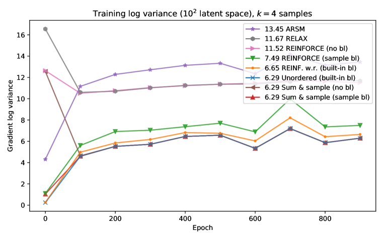
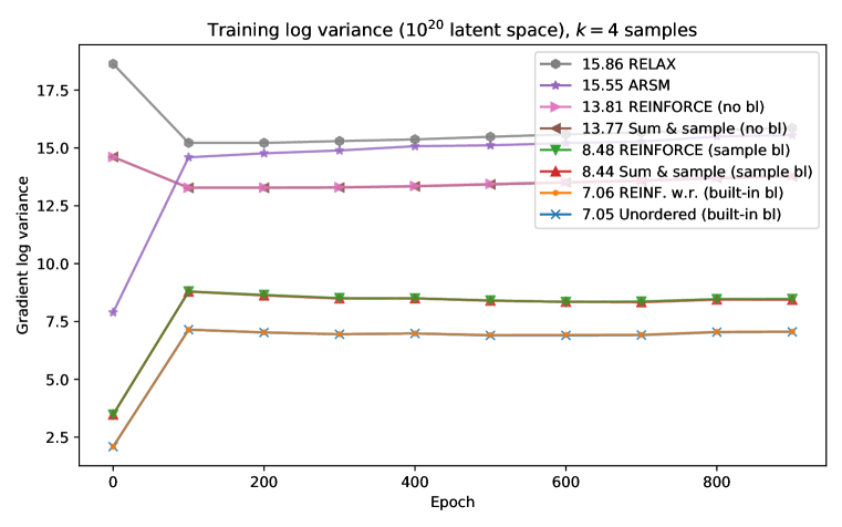
Refer to caption
(a) Small domain (latent space size 102superscript10210^{2})
Refer to caption
(b) Large domain (latent space size 1020superscript102010^{20})
Figure 4: Gradient log variance of different unbiased estimators with k=4π‘˜4k=4 samples, estimated every 100 (out of 1000) epochs while training using REINFORCE with replacement. Each estimator is computed 1000 times with different latent samples for a fixed minibatch (the first 100 records of training data). We report (the logarithm of) the sum of the variances per parameter (trace of the covariance matrix). Some lines coincide, so we sort the legend by the last measurement and report its value.
Refer to caption
(a) Small domain (latent space size 102superscript10210^{2})
Refer to caption
(b) Large domain (latent space size 1020superscript102010^{20})
Figure 5: Smoothed validation -ELBO curves during training of two independent runs when with different estimators with k=1π‘˜1k=1, 4 or 8 (thicker lines) samples (ARSM has a variable number). Some lines coincide, so we sort the legend by the lowest -ELBO achieved and report this value.
Negative ELBO on validation set.

Figure 5 shows the -ELBO evaluated during training on the validation set. For the large latent space, we see validation error quickly increase (after reaching a minimum) which is likely because of overfitting (due to improved optimization), a phenomenon observed before (Tucker etΒ al., 2017; Grathwohl etΒ al., 2018). Note that before the overfitting starts, both REINFORCE without replacement and the unordered set estimator achieve a validation error similar to the other estimators, such that in a practical setting, one can use early stopping.

Results using standard binarized MNIST dataset.

Instead of using the MNIST dataset binarized by thresholding values at 0.5 (as in the code and paper by Yin etΒ al. (2019)) we also experiment with the standard (fixed) binarized dataset by Salakhutdinov & Murray (2008); Larochelle & Murray (2011), for which we plot train and validation curves for two runs on the small and large domain in Figure 6. This gives more realistic (higher) -ELBO scores, although we still observe the effect of overfitting. As this is a bit more unstable setting, one of the runs using REINFORCE with replacement diverged, but in general the relative performance of estimators is similar to using the dataset with 0.5 threshold.
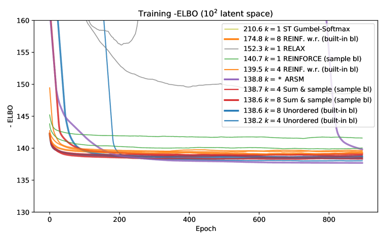
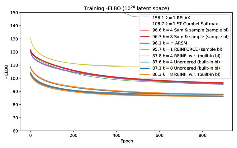
Refer to caption
(a) Training -ELBO, small domain (102superscript10210^{2})
Refer to caption
(b) Training -ELBO, large domain (1020superscript102010^{20})
Refer to caption
(c) Validation -ELBO, small domain (102superscript10210^{2})
Refer to caption
(d) Validation -ELBO, large domain (1020superscript102010^{20})
Figure 6: Smoothed training and validation -ELBO curves during training on the standard binarized MNIST dataset (Salakhutdinov & Murray, 2008; Larochelle & Murray, 2011) of two independent runs when with different estimators with k=1π‘˜1k=1, 4 or 8 (thicker lines) samples (ARSM has a variable number). Some lines coincide, so we sort the legend by the lowest -ELBO achieved and report this value.

Appendix H Travelling Salesman Problem

The Travelling Salesman Problem (TSP) is a discrete optimization problem that consists of finding the order in which to visit a set of locations, given as x,yπ‘₯𝑦x,y coordinates, to minimize the total length of the tour, starting and ending at the same location. As a tour can be considered a sequence of locations, this problem can be set up as a sequence modelling problem, that can be either addressed using supervised (Vinyals etΒ al., 2015) or reinforcement learning (Bello etΒ al., 2016; Kool etΒ al., 2019a).

Kool etΒ al. (2019a) introduced the Attention Model, which is an encoder-decoder model which considers a TSP instances as a fully connected graph. The encoder computes embeddings for all nodes (locations) and the decoder produces a tour, which is sequence of nodes, selecting one note at the time using an attention mechanism, and uses this autoregressively as input to select the next node. In Kool etΒ al. (2019a), this model is trained using REINFORCE, with a greedy rollout used as baseline to reduce variance.

We use the code by Kool etΒ al. (2019a) to train the exact same Attention Model (for details we refer to Kool etΒ al. (2019a)), and minimize the expected length of a tour predicted by the model, using different gradient estimators. We did not do any hyperparameter optimization and used the exact same training details, using the Adam optimizer (Kingma & Ba, 2015) with a learning rate of 10βˆ’4superscript10410^{-4} (no decay) for 100 epochs for all estimators. For the baselines, we used the same batch size of 512, but for estimators that use k=4π‘˜4k=4 samples, we used a batch size of 5124=1285124128\frac{512}{4}=128 to compensate for the additional samples (this makes multi-sample methods actually faster since the encoder still needs to be evaluated only once).