How should we choose the boundary conditions in a simulation which could detect anyons in one and two dimensions?
Abstract
We discuss the problem of anyonic statistics in one and two spatial dimensions from the point of view of statistical physics. In particular we want to understand how the choice of the Born-von Karman or the twisted periodic boundary conditions necessary in a Monte Carlo simulation to mimic the thermodynamic limit of the many body system influences the statistical nature of the particles. The particles can either be just bosons, when the configuration space is simply connected as for example for particles on a line. They can be bosons and fermions, when the configuration space is doubly connected as for example for particles in the tridimensional space or in a Riemannian surface of genus greater or equal to one (on the torus, etc …). They can be scalar anyons with arbitrary statistics, when the configuration space is infinitely connected as for particles on the plane or in the circle. They can be scalar anyons with fractional statistics, when the configuration space is the one of particles on a sphere. One can further have multi components anyons with fractional statistics when the configuration space is doubly connected as for particles on a Riemannian surface of genus greater or equal to one. We determine an expression for the canonical partition function of hard core particles (including anyons) on various geometries. We then show how the choice of boundary condition (periodic or open) in one and two dimensions determine which particles can exist on the considered surface. In the conclusion, we mention the Laughlin wavefunction and give a few comments about experiments.
pacs:
02.20.-a,02.40.Pc,02.40.Re,05.30.PrI Introduction
For the statistical mechanics of a systems of many anyons very partial results can be obtained, because the exact solution of a gas of anyons is not known. In fact, in contrast to the bosonic or fermionic case where the statistics is implemented by hand on the many body Hilbert space by constructing completely symmetric or antisymmetric products of single particle wave functions, for anyons the complicated boundary conditions for the interchange of any two particles require the knowledge of the complete many-body configurations. Only the two-body problem is exactly soluble for anyons, and hence only the two-body partition function can be computed exactly. Since the thermodynamic limit cannot be performed, one has to resort to approximate or alternative methods to study the statistical mechanics of anyons Ouvry (2007); Stern (2008). For example if the thermodynamic functions are analytic in the particle density, it is well-known that the low density, or equivalently the high temperature limit, of a (free) gas can be investigated using the virial expansion.
Anyons have had important physical applications and it would be wrong to convey the idea that they are just mathematical fantasies. For example physical objects which can be described as anyons are the quasi-particle and quasi-hole excitations of planar systems of electrons exhibiting the fractional quantum Hall effect (QHE) (for a review see for instance Prange and Girvin (1990)). Most of the great interest that anyonic theories have attracted in the past few years derives precisely from their relevance to a better understanding of the fractional QHE Halperin (1984), in conjunction with several claims that anyons can provide also a non-standard explanation of the mechanism of high temperature superconductivity Chen et al. (1989). Even if recent experiments have cast some shadow on the relevance of fractional statistics to the observed high temperature superconductivity Lyons et al. (1990); Kiefl et al. (1990); Spielman et al. (1990).
In this work we focus on the important problem of how the boundary conditions on the simulation box influences the statistics of the anyonic (see chapter 2 of Ref. Lerda (1992)) particles. We will consider various cases: the infinite line, the circle, the infinite plane, the torus, and the sphere. In each case we will determine the nature of the statistics of the many anyons system. This is important because in a simulation of a real material one usually chooses periodic boundary conditions in order to approach the thermodynamic limit.
Another interesting problem is the determination of a spinor for an anyon with a given rational or even irrational (either algebraic or even transcendental) statistics. If the spin-statistics theorem Pauli (1940) which states that, as a consequence of Lorentz invariance and of locality, half integer spin particles must obey to Fermi statistics and integer spin particles must obey to Bose statistics, there is nothing similar for anyonic statistics Oeckl (2001). Citing Wilczek Wilczek (1990) we can say that “The basic difficulty, which makes this problem much more difficult for generic anyons than for bosons or fermions, is that for generic anyons the many-body Hilbert space is in no sense the tensor product of the one-particle Hilbert space. This circumstance can be understood in various ways. Its root is that in the general case the weighting supplied by anyon statistics depends not only on the initial and final states, but also on a (topological) property of the trajectory connecting them. This means that in the general case it is impossible to summarize the effect of quantum statistics by projection on the appropriate weighted states, as we do for bosons and fermions – where, of course, we project respectively on symmetric and antisymmetric states”. We will consider this problem in a future work.
II The statistical physics anyon problem in two dimensions
The statistical mechanical properties of a quantum system of hard core particles in a volume in spatial dimensions occupying positions and described by an Hamiltonian in thermal equilibrium at the inverse temperature , with the Boltzmann constant and the absolute temperature, are obtainable from the thermal density matrix operator Wu (1984),
| (1) |
In the configurations space representation the thermal density matrix can be written using the following path integral notation,
| (2) |
where is the classical Hamiltonian of the hard core, identical particles. The meaning of and of the phases will be shown in the next two sections.
The canonical partition function can then be found from the trace of the density matrix,
| (3) |
II.1 and its fundamental group
Consider a system of identical hard core particles moving in the euclidean -dimensional space, . A configuration of such a system is clearly specified by the coordinates of the particles, i.e. by an element of . However because of the hard core assumption, any two particles cannot occupy the same position. So from we have to remove the diagonal,
| (4) |
Furthermore our particles are identical and indistinguishable, so we should identify configurations which differ only in the ordering of the particles. In other words we should divide by the permutation group . Therefore we conclude that the configuration space for our system is
| (5) |
To find the fundamental group of such space is a standard problem in algebraic topology, which was solved in the early 60’s Fadell and Neuwirth (1962); Fox and Neuwirth (1962); Fadell and Buskirk (1962). It turns out that the fundamental group of is given by
| (8) |
where is Artin’ s braid group of objects which has the permutation group as a homomorphic image Artin (1926, 1947).
Even from this formal point of view we see that there is a crucial difference between two and three or more dimensions. To have a more explicit understanding of (8), let us consider a two particle example in the light of what we have just observed. Let us start with the case of two dimensions. Instead of assigning the position vectors and for the two particles, is more convenient to introduce the center of mass coordinate,
| (9) |
and the relative coordinate,
| (10) |
We have removed the origin because of the hard core requirement. Since is invariant under the permutations of , we can write,
| (11) |
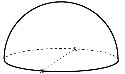
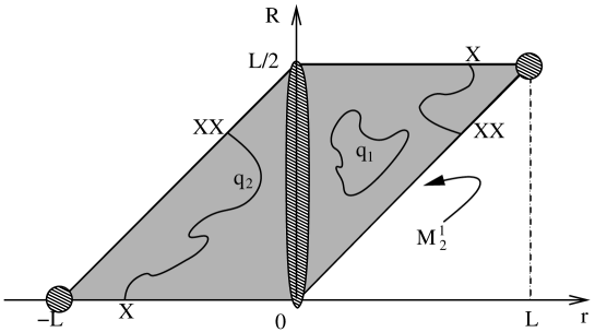
where is some space describing the two degrees of freedom of the relative motion. We now argue that has the topology of a cone. Since two configurations which differ only in the ordering of the particle indexes are indistinguishable, and must be identified. The space is then the upper half plane without the origin and with the positive x-axis identified with the negative one, i.e. is a cone without the tip (see fig. 1).

According to the decomposition (11), any loop in can be classified by the number of times it winds around the cone . Two loops and with different winding numbers are homotopically inequivalent: it is not possible to deform one into the other since the vertex of the cone has been removed. Thus the space and , are infinitely connected, and,
| (12) |
It is important to realize that if the vertex of the cone were included (i.e. allowing particles to occupy the same position in space) the configuration space would be simply connected. Any loop, even when winding around the cone, would be contracted to a point by deforming and unwinding it through the tip. Thus, if we do not impose the hard core constraint on the particles, we can describe only bosonic statistics.
Let us now turn to the case of two particles in three dimensions. After introducing the center of mass coordinate , we can decompose the configurations space as,
| (13) |
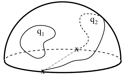
where the space describes the three degrees of freedom of the relative motion. These are the length and the two angles of the relative coordinate . As before and are identified. It is easy to realize that is just the product of the semi-infinite line describing and the projective space describing the orientation of . In turn can be described as the northern hemisphere with opposite points on the equator being identified (see fig. 2).
The space is doubly connected and admits two classes of loops: those which can be shrunk to a point by a continuous transformation and those which cannot. In fig. 3 we exhibit a typical contractible loop and a typical non-contractible loop .
Therefore from the decomposition (13) and the topology of , we deduce that,
| (14) |
Thus only bosons and fermions can exist, the former corresponding to contractible loops and the latter to non-contractible loops.
We have seen that at the heart of the anyonic statistics there is the braid group in place of the permutation group which is responsible for ordinary statistics. There are only two one dimensional unitary representations of , namely the identical one, (bosonic statistics) and the alternating one, , (fermionic statistics). Whereas the braid group admits a whole variety of one dimensional 111When dealing with non-scalar quantum mechanics, i.e. when the wave functions are multiplets instead of one component objects as assumed in the discussion, appropriate higher dimensional representations of would be necessary. unitary representations whose labeling parameter will be identified with the parameter also called the statistics.
II.2 Statistical mechanics problem
One is usually interested in calculating the partition function of the system which is given by the trace of the density matrix. So we choose , or loops in . Two loops are considered equivalent (or homotopic) if one can be obtained from the other by a continuous deformation. All homotopic loops are grouped into one class and the set of all such classes is called the fundamental group and is denoted by 222In the set one can define a product in a very simple and natural way: if and are two classes with representatives path and , then is the class whose representative is the path (that is the pat followed by the path ). It can be shown that this product furnishes with a group structure.. Thus an element of is simply the set of all loops in which can be continuously deformed into each other. On the other hand, loops belonging to two different elements of cannot be connected by a continuous transformation. Naturally has to be a real positive probability function.
In order for (2) to make sense as a probability amplitude, the complex weights cannot be arbitrary. In fact, since we want to maintain the usual rule for combining probabilities,
| (15) |
the weights must satisfy,
| (16) |
for any and . Equation (16) can also be read as the statement that must be a one dimensional unitary () representation of the fundamental group Laidlaw and Witt (1971). To see which representations are possible, we have to specify better what is and its fundamental group.
This means that we have to look for one dimensional unitary representations of the fundamental group, i.e.
| (17) |
or in the notation used by F. Wilczek Wilczek (1990), and where is the winding number and the relative angular momentum in units of quantized in units of in each sector .
In there are only possible representations of the permutation group: the one corresponding to the bosonic statistics ( mod 2) and the one corresponding to the fermionic statistics ( mod 2). In one has to choose representations of the braid group (see chapter 2 of Ref. Lerda (1992)) and the statistical parameter can be arbitrary at least in principle 333There are restrictions on coming from the topology of the two dimensional space. For example for particles moving on a torus (or a 2D box with periodic boundary conditions), can only be a rational number (see Section III.0.4).. Particles with this property are called anyons. In it is not enough to specify the initial and final configurations to completely characterize the system; it is also necessary to specify how the different trajectories wind or braid around each other. In other words the time evolution of the particles is important and cannot be neglected in . This fact implies that in order to classify and characterize anyons, the representations of the permutation group must be replaced by those of the more complicated braid group.
The following is always true (here and are two different imaginary times),
| (18) |
where the symbol denotes the azimuthal angle of particle with respect to particle and is an integer. This can be interpreted by saying that to complete a loop in configuration space an integer number of exchanges is always necessary. And one can write (see chapter 2 of Ref. Lerda (1992))
| (19) |
being the Cartesian coordinates of the particle.
So we can be formally express
| (20) |
Notice that the functions , where represents an arbitrary braiding (see chapter 2 of Ref. Lerda (1992)) are in general very complicated and can be specified only when the dynamics of the particles is fully taken into account. However the formal definition (20) may come useful when inserted into the density matrix expression (II.2). So that the expression for the diagonal of the density matrix gets the suggestive form,
Expression (II.2) tells us that instead of dealing with anyons governed with the Hamiltonian , we can work with bosons whose dynamics is dictated by the new Hamiltonian . In particular we could treat fermions governed by an Hamiltonian as bosons with a “fictitious” Hamiltonian . Notice that this statistical interaction is very peculiar and intrinsically topological in nature (it is actually a total derivative). Its addition to the Hamiltonian does not change the equations of motion, which are a reflection of the local structure of the configuration space, but does change the statistical properties of the particles, which are instead related to the global topological structure of the configuration space (it can be locally realized as a gauge theory with a Chern-Simons kinetic term).
Now since has to be a real positive function as well as all the one has to add the constraints
| (22) | |||
| (23) |
III Periodic boundary conditions
The configuration space of identical hard core two dimensional particles has a non trivial topology.
-
•
If the particles are free to move in or in a finite box then the configuration space is infinitely connected (see fig. 1). Its fundamental group is the braid group whose representations are labeled by an arbitrary parameter . This unusual statistics can be implemented on ordinary particles (for instance bosons) by the addition of a topological statistical interaction as we saw in Eq. (II.2).
-
•
If the particles are free to move in a finite box with periodic boundary conditions, a torus, a compact Riemannian surface of genus 1, then only bosons and fermions are possible Lerda (1992) if the multi-particle wavefunctions carry a one dimensional (appropriate for scalar wave functions) unitary representation of the braid group. However anyons are possible even on a torus provided that wave functions with many components are considered, as for example for spin one-half electrons. In this case one has to look at higher dimensional representations of the braid group which lead to the concepts of generalized fractional statistics and generalized anyons Einarsson (1990, 1991); Imbo and March-Russell (1990); Wen (1990). Now only fractional statistics are possible and can only be a rational number, with and coprime integers and where is a non negative integer. This is essentially due to the requirement to have nonzero winding numbers along the two periods (the two handles) of the torus: one periodicity winding acts on a wave function with components by multiplying all components by the same phase factor, while the other periodicity winding mix among themselves the components of the wave function (at the end of chapter 2 of Ref. Lerda (1992) the general case of a Riemannian surface of a generic genus is also made).
In order to avoid periodic boundary conditions one could work on the surface of a sphere, in this case scalar anyons with fractional statistics will emerge Lerda (1992).
So this poses the following conceptual problem. If one is to simulate, for example through the Monte Carlo technique, a system of identical hard core particles living in two dimensions, he should use, for the many body wave function of the system contained in a two-dimensional box of sides and , either the Born-von Karman periodic boundary conditions
| (24) |
with and or the twisted boundary conditions Lin et al. (2001), with , to mimic the thermodynamic limit. Then the fractional statistics or the anyonic nature of the particles is necessarily changed by the topological change of the configurational space. Moreover as we will discuss in the conclusions the twisted boundary conditions, even if they do not alter the qualitative picture respect to the Born-von Karman boundary conditions, regarding the topological properties of the underlying configurational space, they become essential in the description of anyons or the fractional QHE (see Lerda (1992) chapter 4). We can in fact say that in the interchange of two particles each one of the two changes identity when winding across the boundary (24) as follows,
| (25) |
Since the discovery of the twisted boundary conditions by Chang Lin et al. in 2001 to optimize the approach to the thermodynamic limit of a generic Monte Carlo simulation of a many-body system we are unaware of their use in computer experiment for anyons as in Eq. (25).
Let us now reduce ourselves to the case. We have seen that when the particles are free to move on all then the center of mass coordinate splits off in a trivial way. Let’ s see what we can easily say about the configuration spaces of particles confined in a box (B) or in a periodic box (PB). We start with a one dimensional space and then study the two dimensional one.
III.0.1 For a box in [1d-B]
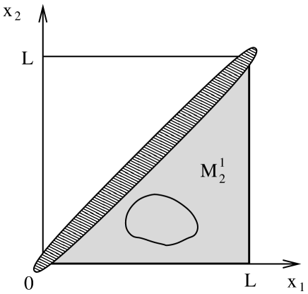
Call and the particles coordinates. In this case (see fig. 4),
| (26) |
which is simply connected. So only boson statistics is allowed.
We could, as well, have introduced the center of mass coordinate and the relative coordinate . Using this coordinates (see fig. 5).
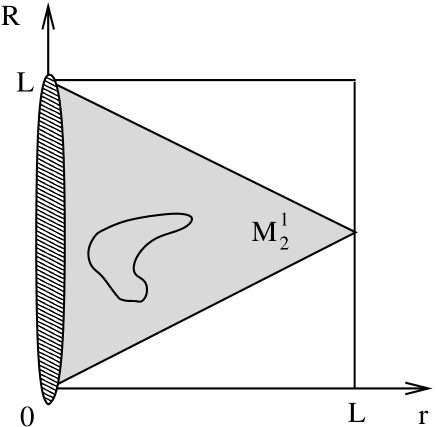
As expected again is simply connected.
III.0.2 For a box with periodic boundary conditions in [1d-PB]
We now consider the case of particles on a circle of length . Using the center of mass coordinate and the relative coordinate one sees by inspection that,
| (27) |
which is infinitely connected (as shown in fig. 6 two loops with different winding around the missing point are homotopically inequivalent). So anyons with arbitrary statistics is allowed.
The same thing can be seen introducing the center of mass angle and the relative angle (see fig. 7).
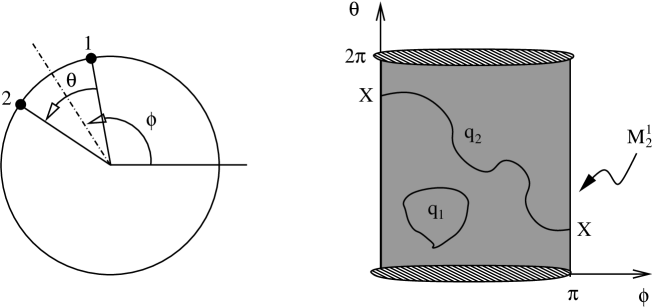
The rectangle in the plane defined by and includes all possible configurations, except for the left and right edges where and both represent the same configuration. Because of this identification the rectangle becomes a Möbious band which is still infinitely connected. In this case though even with a multi-component wave function the statistics must remain arbitrary and not fractionary as in the two dimensional one since we have only one periodicity.
III.0.3 For a box in [2d-B]
Using the same argument used for the [1d-B] we can say that where is a space with the same topology as the cone without the tip introduced in the case of particles without boundaries. The only difference being that the cone now does not extend to infinity but is finite and its height depends on . So once again, since is infinitely connected, also is. And anyon statistics is allowed with arbitrary .
III.0.4 For a box with periodic boundary conditions in [2d-PB]
In this case we can say that something similar was happening from going from the 2d plane ( infinitely connected) to the 3d space ( doubly connected). Now in [1d-PB] M is infinitely connected and in [2d-PB] is doubly connected. We split again into the product of the center of mass configuration space and of the two impenetrable particles relative coordinates one, . It turns out that now, due to the periodic boundary conditions, is a cone without the tip, of finite height, as in Fig. 1, and with the end points of a diameter of the base identified. This is a doubly connected space. All this is only true if we consider scalar wave functions, i.e. one dimensional representations of the fundamental group of the configuration space. For wave functions with many components the generators of the representations of the fundamental group of the configuration space are such that Lerda (1992) a rational number, with and coprime numbers and a restriction on the total number of particles, , where is a non negative integer. For an extensive discussion of anyons on compact surfaces and on the torus in particular, we refer the reader to the review by R. Iengo and K. Lechner Iengo and Lechner (1992).
IV Conclusions
Twisted boundary conditions play a relevant role in the anyons problem where the topology of the underlying configuration space determines the statistics of the particles. We review various cases. For scalar many body wave functions on the segment or the infinite line one can have only bosons, on the circle one can only have anyons with arbitrary statistics, on the square or the infinite plane one can also have only anyons with arbitrary statistics, and on the torus which has two periodicities only bosons and fermions are allowed as on the infinite three dimensional Euclidean space. We gave a proof of these different behaviors for just a two-body system. This is enough to determine the anyonic symmetry of the many-body wave function as we discussed in Section II.2 but one cannot exclude other kinds of three and higher body symmetries where it is necessary to substitute of Eq. (19) with a different . We gave proofs of these circumstances based on the geometrical topological properties of the configurational space in each case, which we regard as the simplest way to proceed.
If we allow for a many components wave function on the torus we may have anyons but with only fractional statistics which proved to give an interpretation for the fractional QHE. In this case a series of new states of matter emerge as incompressible quantum liquids Laughlin (1983a, b) around which the low-energy excitations are localized quasi-particles with unusual fractional quantum numbers, i.e. anyons. The Laughlin variational ground-state wave functions requires the statistics, , to be an odd integer whereas the excited states require it to be rational. Laughlin chooses the trial ground-state wave function of the Bijl-Dingle-Jastrow product form
| (28) |
where is the magnetic length, the magnetic field orthogonal to the metallic plate, is the complex coordinate of the i-th electron and is a normalization factor. Since is an odd integer, is totally antisymmetric, and so it describes ordinary fermions. The prefactor is also of the Jastrow type: it has a zero of order at coincident points , showing that electrons tend very strongly to repel each other in a way that is appropriate to minimize the Coulomb interaction. If goes around by an angle the wave function acquires a phase , as if each particle carried units of flux. This allows Laughlin to use the fact that the can be interpreted as the Boltzmann factor of a One Component Plasma of classical particles of charge living in two dimensions where the neutralizing background has a surface charge density at an inverse temperature . The coupling constant of the plasma is and its properties are available exactly analytically at the special value of the coupling constant Jancovici (1981); Fantoni et al. (2003); Fantoni and Telléz (2008) when the two dimensional electron gas corresponds to a full Landau level (see Ref. Lerda (1992) chapter 8).
A word of caution when thinking at the physical implications of all this are nonetheless necessary. From a purely conceptual point of view the fact that in order to have a fractional statistics one has to impose twisted periodic boundary conditions that are an artificial means to approach the thermodynamic limit and have no physical meaning sheds some doubts on the relevance of the anyonic theory on the interpretation of the fractional QHE. From the point of view of the numerical experiment the presence of a magnetic field implies that the ground state wave function will, in general, be complex valued and in order to deal with the symmetry given by the anyonic statistics one should use methods similar to the ones used in Ref. Zhang et al. (1993); Jones et al. (1997). Also we proposed to combine these methods with the twisted boundary conditions first employed in 2001 by Chang Lin et al. Lin et al. (2001) for a generic many-body system. It would be desirable to perform the simulation on a sphere with a Dirac magnetic monopole at the center Melik-Alaverdian et al. (2001) in order to be able to simulate scalar anyons with fractional statistics, without the necessity of implementing any sort of boundary conditions.
Another issue in disfavor of the description of the physically observed QHE is the fact that in a laboratory the electrons will surely not be exactly living in a two dimensional world but one deals rather with a quasi two dimensional, very very thin, metallic layer Fantoni (2012a) at the interface between two different semiconductors or between a semiconductor and an insulator even if the low temperature and the strong magnetic field freeze the motion along the direction perpendicular to the layer (something similar as explained in the satirical novella by the English schoolmaster Edwin Abbott Abbott: “Flatland: A Romance of Many Dimensions” first published in 1884 by Seeley & Co. of London). This of course would modify also the Coulomb potential of interaction between the electrons from one to one , with the separation between electrons, which are in any case both divergent at . Naturally the Coulomb repulsion is essential to give the incompressibility condition avoiding two particles to overlap.
The real experiment is too complicated to describe in its completeness so one has to resort to approximations and the approximation of considering the electrons as “living” in a two dimensional world with periodic twisted boundary conditions seems to be an effective one. There are many experiments in the field. One I am most interested in is Ref. Jaime et al. (1997) where it is shown that the sign of the Hall effect in the transport properties of doped lanthanum manganites films for small polaron Fantoni (2012b, 2013) hopping can be “anomalous”. A small polaron based on an electron can be deflected in a magnetic field as if it were positively charged and, conversely, a hole-based polaron can be deflected in the sense of a free electron. Measurements of the high-temperature Hall coefficient of manganite samples reveal that it exhibits Arrhenius behavior and a sign anomaly relative to both the nominal doping and the thermoelectric power. The results are discussed in terms of an extension of the Emin-Holstein theory of the Hall mobility in the adiabatic limit.
There are now several proposed experiments aimed at identifying the existence of non-Abelian statistics in nature. Non-Abelian phases are gapped phases of matter in which the adiabatic transport of one excitation around another implies a unitary transformation within a subspace of degenerate wavefunctions which differ from each other only globally Read and Moore (1992).
Another more recent experimental interest in anyons is for topological quantum computation Stern (2010); von Keyserlingk et al. (2015): Systems exhibiting non-Abelian statistics can store topogically protected qubits Sarma et al. (2005).
Acknowledgements.
I would like to acknowledge fruitful discussions with Rob Leigh, Eduardo Fradkin, Michael Stone, and last but not least Myron Salamon who showed me the physics of calorimeters, way back in 2000 in Urbana.References
- Ouvry (2007) S. Ouvry, Séminaire Poinacré XI, 77 (2007).
- Stern (2008) A. Stern, Annals of Physics 323, 204 (2008).
- Prange and Girvin (1990) R. Prange and S. Girvin, The Quantum Hall Effect, edited by R. Prange and S. Girvin (Springer-Verlag, Berlin, 1990).
- Halperin (1984) B. Halperin, Pys. Re. Lett. 52, 1583 (1984).
- Chen et al. (1989) Y.-H. Chen, F. Wilczek, E. Witten, and B. Halperin, Int. Jour. Mod. Phys. B3, 1001 (1989).
- Lyons et al. (1990) K. Lyons, J. Kwo, J. D. Jr., G. Espinosa, M. McGlashan-Powell, A. Ramirez, and L. Schneemeyers, Phys. Rev. Lett. 64, 2949 (1990).
- Kiefl et al. (1990) R. Kiefl, J. Brewer, I. Affieck, J. Carolan, W. H. P. Dosanjh, T. Hsu, R. Kadono, J. Kempton, S. Kreitzman, A. O. Q. Li, T. Riseman, P. Schleger, P. Stamp, H. Zhou, G. L. L.P. Le, B. Sternlieb, Y. Venmra, H. Hart, and K. Lay, Phys. Rev. Lett. 64, 2082 (1990).
- Spielman et al. (1990) S. Spielman, K. Fesler, C. Eom, T. Geballe, M. Fejer, and A. Kapitulnik, Phys. Rev. Lett. 65, 123 (1990).
- Lerda (1992) A. Lerda, Anyons. Quantum mechanics of particles with fractional statistics, Lecture Notes in Physics (Springer-Verlag, Berlin Heidelberg, 1992).
- Pauli (1940) W. Pauli, Phys. Rev. 58, 716 (1940).
- Oeckl (2001) R. Oeckl, Journal of Geometry and Physics 39, 233 (2001).
- Wilczek (1990) F. Wilczek, Fractional Statistics and anyon superconductivity (World Scientific, Singapore, 1990).
- Wu (1984) Y. S. Wu, Phys. Rev. Lett. 53, 111 (1984).
- Fadell and Neuwirth (1962) E. Fadell and L. Neuwirth, Math. Scand. (1962).
- Fox and Neuwirth (1962) R. Fox and L. Neuwirth, Math. Scand. 10, 119 (1962).
- Fadell and Buskirk (1962) E. Fadell and J. V. Buskirk, Duke Math. J. 29, 243 (1962).
- Artin (1926) E. Artin, Abh. Math. Sem. Hamburg 4, 47 (1926).
- Artin (1947) E. Artin, Annals of Math. (1947).
- Note (1) When dealing with non-scalar quantum mechanics, i.e. when the wave functions are multiplets instead of one component objects as assumed in the discussion, appropriate higher dimensional representations of would be necessary.
- Note (2) In the set one can define a product in a very simple and natural way: if and are two classes with representatives path and , then is the class whose representative is the path (that is the pat followed by the path ). It can be shown that this product furnishes with a group structure.
- Laidlaw and Witt (1971) M. G. G. Laidlaw and M. D. Witt, Phys. Rev. D (1971).
- Note (3) There are restrictions on coming from the topology of the two dimensional space. For example for particles moving on a torus (or a 2D box with periodic boundary conditions), can only be a rational number (see Section III.0.4).
- Einarsson (1990) T. Einarsson, Phys. Rev. Lett. 64, 1995 (1990).
- Einarsson (1991) T. Einarsson, Mod. Phys. Lett. B5, 675 (1991).
- Imbo and March-Russell (1990) T. Imbo and J. March-Russell, Phys. Lett. 252B, 84 (1990).
- Wen (1990) X.-G. Wen, Phys. Rev. Lett. (1990).
- Lin et al. (2001) C. Lin, F. H. Zong, and D. M. Ceperley, Phys. Rev. E 64, 016702 (2001).
- Iengo and Lechner (1992) R. Iengo and K. Lechner, Phys. Rep. 213, 179 (1992).
- Laughlin (1983a) R. Laughlin, Phys. Rev. Lett. 50, 1395 (1983a).
- Laughlin (1983b) R. Laughlin, Phys. Rev. B B23, 3383 (1983b).
- Jancovici (1981) B. Jancovici, Phys. Rev. Lett. 46, 386 (1981).
- Fantoni et al. (2003) R. Fantoni, B. Jancovici, and G. Téllez, J. Stat. Phys. 112, 27 (2003).
- Fantoni and Telléz (2008) R. Fantoni and G. Telléz, J. Stat. Phys. 133, 449 (2008).
- Zhang et al. (1993) L. Zhang, G. Canright, and T. Barnes, in Computer Simulation Studies in Condensed-Matter Physics VI, Springer Proceedings in Physics, Vol. 76, edited by D. P. Landau, K. K. Mon, and H.-B. Schüttler (Springer-Verlag, Heidelberg, 1993) pp. 199–203.
- Jones et al. (1997) M. D. Jones, G. Ortiz, and D. M. Ceperley, Phys. Rev. E 55, 6202 (1997).
- Melik-Alaverdian et al. (2001) V. Melik-Alaverdian, G. Ortiz, and N. E. Bonesteel, J. Stat. Phys. 104, 449 (2001).
- Fantoni (2012a) R. Fantoni, Regole di somma in un gas di elettroni stratificato, edited by R. Fantoni (Gruppo Editoriale l’ Espresso S.p.A., Roma, 2012) Laurea thesis at ”Scuola Normale Superiore” in Pisa (1995). Advisor: M. P. Tosi, ISBN 978-889-101-539-6.
- Jaime et al. (1997) M. Jaime, H. T. Hardner, M. B. Salamon, M. Rubinstein, P. Dorsey, and D. Emin, Phys. Rev. Lett. 78, 951 (1997).
- Fantoni (2012b) R. Fantoni, Phys. Rev. B 86, 144304 (2012b).
- Fantoni (2013) R. Fantoni, Physica B 412, 112 (2013).
- Read and Moore (1992) N. Read and G. Moore, Prog. Theor. Phys. Suppl. 107, 157 (1992).
- Stern (2010) A. Stern, Nature 464, 187 (2010).
- von Keyserlingk et al. (2015) C. W. von Keyserlingk, S. H. Simon, and B. Rosenow, Phys. Rev. Lett. 115, 126807 (2015).
- Sarma et al. (2005) S. D. Sarma, M. Freedman, and C. Nayak, Phys. Rev. Lett. 94, 166802 (2005).