Kinetic Geodesic Voronoi Diagrams
in a Simple Polygon
Abstract
We study the geodesic Voronoi diagram of a set of linearly moving sites inside a static simple polygon with vertices. We identify all events where the structure of the Voronoi diagram changes, bound the number of such events, and then develop a kinetic data structure (KDS) that maintains the geodesic Voronoi diagram as the sites move. To this end, we first analyze how often a single bisector, defined by two sites, or a single Voronoi center, defined by three sites, can change. For both these structures we prove that the number of such changes is at most , and that this is tight in the worst case. Moreover, we develop compact, responsive, local, and efficient kinetic data structures for both structures. Our data structures use linear space and process a worst-case optimal number of events. Our bisector and Voronoi center kinetic data structures handle each event in time. Both structures can be extended to efficiently support updating the movement of the sites as well. Using these data structures as building blocks we obtain a compact KDS for maintaining the full geodesic Voronoi diagram.
1 Introduction
Polygons are one of the most fundamental objects in computational geometry. As such, they have been used for many different purposes in different contexts. Within the path planning community, polygons are often used to model different regions. A simple example is planning the motion of a robot in a building: we can model all possible locations that a robot can reach by a polygon (the walls or other obstacles would define its boundary). Then, the goal is to find a path that connects the source point with its the destination and that minimizes some objective function. There are countlessly many results that depend on the exact function used (distance traveled [15], time needed to reach a destination [22], number of required turns [33], etc.)
Paths that minimize distance are often called geodesics. In this paper, we consider one of the most natural metrics: the domain is a simple polygon and paths are constrained to stay within the closure of . Under this setting it is well known that given two points there exists a unique geodesic connecting the two points. Moreover, is a simple polygonal chain whose vertices (other than the first and last) are reflex vertices of . Thus, we define the geodesic distance function between and as the the sum of Euclidean lengths of the segments in . With the properties mentioned above, it follows that the geodesic distance is a proper distance and is well defined [22].
Once the metric is fixed, many different problems can be considered. Two of the most basic problems are the computation of shortest path maps and augmented Voronoi diagrams. A shortest path map (or SPM for short) is a partition of the space into maximal connected regions so that points in the same region travel in the same way to the fixed source [15, 18].
Similar to shortest paths, there are several ways in which paths can be considered “in the same way”. For the purposes of this paper, we use the well established combinatorial approach: recall that geodesics are simple polygonal chains, thus is described as the union of segments for some . Two paths and are (combinatorially) equivalent if and only if and . In other words, both paths traverse through the same sequence of intermediate polygon vertices (note that both start and end could be different). Note that if two paths are combinatorially equivalent, then they must traverse the same vertices in either the same or reverse order (i.e., the vertex order cannot be rearranged). This holds true because subpaths of shortest paths are always shortest paths. For a full proof of this statement (and more interesting properties of geodesics) we refer the interested reader to the seminal paper by Guibas et al. [15]. From now on, for simplicity in the description, we assume that the vertices of are in general position. That is, any segment contained in the closure passes through at most two vertices. This assumption can be removed using standard data perturbation techniques.
Voronoi diagrams are another fundamental object of computational geometry. Given a collection of sites inside some metric space, the Voronoi diagram is a partition of the space into regions so that points in the same region have the same closest site. These diagrams are often used in facility location problems, but there are many applications in different fields of science (see [10], chapter 7 for a survey of this problem and its many applications).
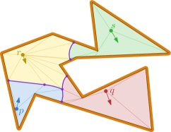
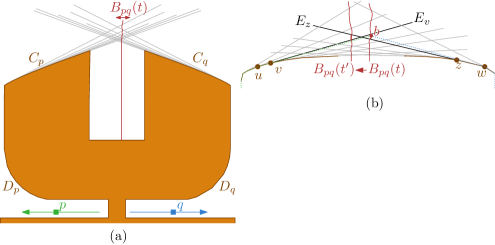
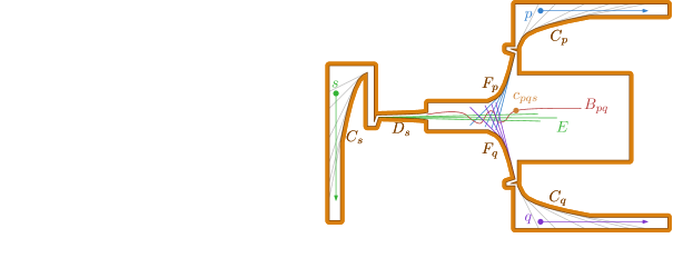
Augmented Voronoi diagrams are a generalization of both shortest path maps and Voronoi diagrams. In our setting, they are defined as follows: given a set of points (which from now on we call sites) inside a simple polygon of vertices, the augmented Voronoi diagram of with respect to is a subdivision of into cells so that points in the same cell have the same closest site and the paths from and to the nearest site are combinatorially equivalent (see Fig. 1 for an illustration).
These diagrams often come naturally in different settings. For example, in the previously mentioned robotics setting where represents the space that the robot can travel to, the sites could be some service location (say, battery stations). Robots move along doing some task, but when they need recharging, they must travel to the nearest charging station. The shortest path can be found with the help of the augmented Voronoi diagram. The main advantage of augmented diagrams is that full paths need not be stored: from the each cell we only need to know the first vertex of the shortest path to its closest site. Once we reach that vertex, we are at a different cell of the augmented Voronoi diagram, so we query the diagram and obtain a new intermediate vertex for the robot. This process is repeated until the robot eventually reaches the charging station.
In this paper we consider another natural extension of these fundamental problems: rather than considering static sites, we want to study the case in which sites can move. In the robotics example, two agents might be trying to meet, or one agent might want to evade the other, or one agent might simply need to meet up with a second one that is performing a different task [21]. The existing static algorithms would need to recompute the diagram after each infinitesimal movement. Instead, in this paper we aim to maintain as much information as possible, doing only local changes whenever strictly necessary. A data structure that can handle such a setting is known as a kinetic data structure (or KDS for short) [8].
1.1 Related Work
In this paper we combine three fundamental properties of the computational geometry community: polygons, Voronoi diagrams, and kinetic data structures. Surprisingly, there is very little work that combines the three results.
Aronov was the first to apply the concept of augmented Voronoi diagram to geodesic environments [4]. This structure has proven to be of critical importance for obtaining efficient solutions to other related problems such as finding center points, closest pairs, nearest neighbors, and constructing spanners [27, 28]. Aronov proved that the augmented Voronoi diagram of a set containing static point sites in a simple polygon of vertices has complexity . Moreover, he presented an time algorithm for constructing , which was improved to by Papadopoulou and Lee [28]. Recently, there have been several improved algorithms [20, 25] which ultimately lead to an optimal time algorithm by Oh [24]. Furthermore, Agarwal et al.[1] recently showed that finding the site in closest to an arbitrary query point — a key application of geodesic Voronoi diagrams — can be achieved efficiently even if sites may be added to, or removed from, .
There are no known results on maintaining an (augmented) geodesic Voronoi diagram when multiple sites move continuously in a simple polygon . In case there is only one site , Aronov et al. [6] presented a KDS that maintains the shortest path map of . Their data structure uses space, and processes a total of events in time each111The original description by Aronov et al. [6] uses a dynamic convex hull data structure that supports time queries and updates. Instead, we can use the data structure by Brodal and Jacob [9] which supports these operations in time.. Karavelas and Guibas [19], provide a KDS to maintain a constrained Delaunay triangulation of . This allows them to maintain the geodesic hull of with respect to , and the set of nearest neighbors in (even in case has holes). Their KDS processes events in time each, where and is the maximum length of a Davenport-Schinzel sequence of symbols of order [31]. Here, and throughout the rest of the paper denotes some small (natural) constant that depends on the algebraic degree of the polynomials describing the movement of the sites. Note that, for any constant , is near linear, and thus is near-constant.
Parallel to this work on geodesic environments, kinetic data structures (KDS) have been used for a wide range of problems in different settings. We refer the reader to the survey by Basch et al. [8] for an overview of these results. Our data structures follows the same framework: points move linearly in a known direction. Each KDS maintains a set of certificates that together certify that the KDS currently correctly represents the target structure. Typically these certificates involve a few objects each and represent some simple geometric primitive. For example a certificate may indicate that three points form a clockwise oriented triangle. As the points move these certificates may become invalid, requiring the KDS to update. This requires repairing the target structure and creating new certificates. Such a certificate failure is called an (internal) event. An event is external if the target structure also changes. The performance of a KDS is measured according to four measures. A KDS is considered compact if it requires little space, generally close to linear, responsive if each event is processed quickly, generally polylogarithmic time, local if each site participates in few events, and efficient if the ratio between external and internal events is small, generally polylogarithmic. Note that for efficiency it is common to compare the worst-case number of events for either case.
Guibas et al. [16] studied maintaining the Voronoi diagram in case and distance is measured by the Euclidean distance. They prove that the combinatorial structure of may change times, and present an a KDS that handles at most events, each in time. Their results actually extend to slightly more general types of movement. It is one of the long outstanding open problems if this bound can be improved [12, 14]. Only recently, Rubin [30] showed that if all sites move linearly and with the same speed, the number of changes is at most for some arbitrarily small . For arbitrary speeds, the best known bound is still . When the distance function is specified by a convex -gon the number of changes is [2].
1.2 Results and paper organization
We present the first KDS to maintain the augmented geodesic Voronoi diagram of a set of sites moving linearly inside a simple polygon with vertices. Our results provide an important tool for maintaining related structures in which the agents (sites) move linearly within the simple polygon (e.g. minimum spanning trees, nearest-neighbors, closest pairs, etc.).
To this end, we prove a tight bound on the number of combinatorial changes in a single bisector, and develop a compact, efficient, and responsive KDS to maintain it (Section 3). Our KDS for the bisector uses space and processes events in time. We then show that the movement of the Voronoi center —the point equidistant to three sites — can also change times (Section 4). We again show that this bound is tight, and develop a compact, efficient, and responsive KDS to maintain . The space usage is linear, and handling an event takes time. Both our KDSs can be made local as well, and therefore efficiently support updates to the movement of the sites. Building on these results we then analyze the full Voronoi diagram of moving sites (Section 5). We identify the different types of events at which changes, and bound their number. Table 1 gives an overview of our bounds. We then develop a compact KDS to maintain .
| Event | Lower bound | Upper bound |
|---|---|---|
| -collapse/expand | ||
| -collapse/expand | ||
| -collapse/expand | ||
| -collapse/expand | ||
| -collapse/expand | ||
| vertex |
2 Preliminaries
Let be a simple polygon with vertices, and let . Let be the shortest path between and that stays entirely inside (we view as a closed polygon and thus such path is known to always exist and to be unique [22]). We measure length of a path by the sum of the Euclidean edge lengths. Such a shortest path is known as a geodesic, and its length as the geodesic distance and is denoted by . From now on, for simplicity in the expression we remove the term geodesic when talking about distances. Thus, any term that depends on an implicit distance (such as closer or circle) refers to the geodesic counterparts (i.e., geodesically closer or geodesic circle).
Let denote the time domain, and let be a set of point sites that each move with a fixed speed and direction in a space . That is, we see each point as a linear function from to . More precisely, let expresses the time interval during which entity moves inside then . In the remainder of the paper, we will not distinguish between a function and its graph. The Voronoi diagram of is a partition of into regions, one per site , such that any point in such a region is closer to than to any other site in . Note that the Voronoi diagram also changes with time (and thus technically ), but we omit the dependency of for simplicity in notation.
General Position
In static domains (i.e., when points do not move), it is common to assume that the input satisfies some form of general position (say, there are no three collinear input vertices). These general position assumptions can often be removed using standard symbolic perturbation techniques (imagine performing an infinitesimally small random perturbation to the input values; we refer the interested reader to [13] for more details on how to implement this without having to modify the input).
Let to denote the union of the set of sites and vertices (recall that vertices are static, thus there is no dependency on ). Along the paper we would like to make the following assumptions:
-
1.
No line contains more than two points of .
-
2.
For any there do not exist more than three of that are geodesically equidistant to .
-
3.
For any there do not exist two distinct points of that are geodesically equidistant to .
Each of these constraints can be expressed with algebraic equations of constant degree, thus they can be achieved on a static set of points using symbolic perturbation. Unfortunately, the same cannot be said when sites move along time: for example, when a point moves fast through the area between two slowly moving points, at some point in time the moving point will align with the other two. In this case, symbolic perturbation can help to split and limit the duration of these degeneracies.
To make this more precise we define the concept of a singular exception. Given a set of moving sites in a simple polygon , we say that a series of algebraic constraints on are satisfied with singular exceptions if all constraints are satisfied for all except a finite number of exceptions , for each there is exactly one constraint that is not satisfied and there is exactly one instance that does not satisfy the constraint (say, at we have exactly one line containing more than two points of ) and, the constraint being violated has exactly one additional point above the allowed limit (i.e., the line of passes through exactly three points of ).
By viewing as lines in three dimensions, the assumptions above with singular exceptions can be expressed algebraically, and thus obtained using symbolic perturbation. As mentioned above, an infinitesimally small but random permutation on the input would guarantee this with high probability (but there is no need to actually modify the input [13]). We note that along the paper we will introduce additional general position assumptions. For simplicity in the description all of them will be with singular exceptions.
Geodesic Voronoi Diagrams
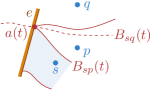
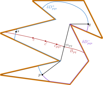
We now review some known properties of geodesic Voronoi diagrams and shortest path maps that we will use. Let be the shortest path map of . For all points in a single region of , the shortest path from has the same internal vertices. Each such region is star-shaped with respect to the last internal vertex on the shortest path. Often it will be useful to refine into triangles incident to (by adding segments between and other vertices of in the same region). We refer to the resulting subdivision of as the extended shortest path map222In order to have a proper subdivision, we would need to consider one or even zero dimensional regions in which points have two or three shortest paths to . For simplicity, we follow a slight abuse done in previous papers and consider each region as closed with nonempty intersection with neighboring cells. In this way, a point with two or three shortest paths to belongs to two or three regions at the same time. This is not a proper subdivision, but simplifies things from a computational perspective.. With some abuse of notation we will use to denote this subdivision as well. Fixed a source and a reflex vertex , the extension segment is defined as follows: shoot a ray from that is parallel to the last edge in and goes away from . Extend that ray until it properly intersects with . Note that this segment could degenerate to a point (see Figure 2). When is not degenerate it splits into two regions, one of which contains . More interestingly, for all points in the other region their shortest path to passes through .
Given two sites and , the bisector is the set of all points that are equidistant to and . If no vertex of lies on the bisector, then is a continuous curve connecting two points on . Moreover, can be decomposed into pieces, each of which is a subarc of a hyperbola (that could degenerate to a line segment [4, 23]). More generally, for sites in general position we have that:
Lemma 1 (Aronov [4]).
consists of vertices with degree 1 or 3, and vertices of degree 2. For each degree 2 vertex there is are so that lies on the bisector and lies on extension segment of or . All edges of are hyperbolic arc segments. Every vertex of contributes at most one extension segment to .
Lemma 2 (Aronov et al. [6]).
Let be a point moving linearly inside a simple polygon with vertices. The extended shortest path map changes at most times.
Lemma 3.
Let be a vertex of , there are time intervals in which has a unique closest site , and the distance from to over time is a hyperbolic function.
Proof.
For every site , consider the distance function from to . The site closest to corresponds to the lower envelope of these functions. Each function consists of pieces, each of which is of the form , for some vertex of . Since is a linear function in , we will argue that two such pieces can intersect at most four times. It then follows that the lower envelope has complexity [31].
Let and be entities moving linearly, each with a constant speed, and consider a time interval during which is the last vertex on , and is the last vertex on . We have to argue that within time interval , the functions and intersect at most four times, hence that has at most four roots. We use that and are linear functions in , and that in this interval , we have that and . By repeated squaring we now obtain a polynomial of degree four. Hence, there are at most four roots. The lemma follows. ∎
3 A Single Bisector
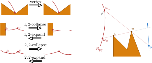
In this section we study the single bisector of a fixed pair of sites and and study how it changes as the points move linearly. Let and be the endpoints of the bisector defined so that lies to the right of when following the bisector from to . As and move the structure of changes at discrete times, or events. We distinguish between the following types of events (see Fig. 3, left):
-
•
vertex events, at which an endpoint of coincides with a vertex of ,
-
•
-collapse events, at which a degree 2 vertex (an interior vertex) of disappears as it collides with a degree 1 vertex (an endpoint),
-
•
-expand events, at which a new degree 2 vertex appears from a degree 1 vertex,
-
•
-collapse events at which a degree 2 vertex disappears by colliding with an other degree 2 vertex, and
-
•
-expand events, at which a new degree 2 vertex appears from a degree 2 vertex.
We now briefly justify that these are all the events that can happen to a single bisector. When the sites are in general position, Aronov [4, Lemma 3.2] showed that the bisector is the concatenation of hyperbolic arcs and line segments that touches the boundary of in two points. Thus, the vertices of the bisector are of degree at most two, and therefore, our characterization of -collapse and expand events in terms of the degrees and of the bisector vertices captures all changes in the interior of the polygon. Furthermore, since the bisector touches the boundary of the polygon only in its two endpoints, the events where the bisector changes due to the polygon boundary are when the endpoint of the bisector coincides with a vertex of the polygon; i.e. at vertex events. Note that, even with general position assumptions, multiple events could happen at the same time and place. An example of this is shown in Fig. 4: the bisector passes through a reflex corner and thus “jumps” from an edge to another. This is in fact the combination of a vertex event and a -expand event. Each time we process an event we check if multiple events are happening, and if so we treat them one at a time.
In our analysis, we will be counting the number of events of each type separately. Note that therefore we are actually double-counting simultaneous events like the one in Fig. 4. In Section 3.1 we prove that there are at most vertex and -collapse events, and at most -collapse events. The number of expand events can be similarly bounded. Despite our double-counting, we can show that our resulting bound on the number of combinatorial changes of is tight in the worst case. In Section 3.2 we then argue that there is a KDS that can maintain efficiently.
3.1 Bounding the Number of Events
We start by showing that the combinatorial structure of a bisector may change times. We then argue that there is also an upper bound on the number of such changes.
Lemma 4.
The combinatorial structure of the bisector can change times.
Proof.
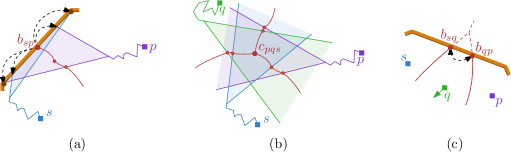
The main idea is to construct two chains of reflex vertices, and , each of complexity , and such that their extension segments (from and , respectively) define a grid of complexity . We then make the bisector sweep across this grid times using two additional chains of reflex vertices and . See Fig. 5(a) for an illustration. Each time sweeps across an intersection point, this causes a combinatorial change, and thus goes through combinatorial changes in total.
The vertices in the chain are almost collinear, so that the region containing the grid of extension segments is tiny. Chain is a mirrored copy of . Let and be two consecutive vertices in , let and be two consecutive vertices in , and consider a time at which and define a segment of the bisector . Hence, for any point on we have . See Fig. 5(b). Once the bisector sweeps over the intersection point of and (from right to left; as is getting closer to the intersection point), this segment collapses into a point, and gets replaced by a segment defined by and (i.e. points equidistant to and for which the shortest paths go have and as last vertex, respectively). Hence, the intersection point corresponds to a combinatorial change in .
Next, we argue that the chains and cause to move back and forth across the grid times. These chains will ensure that and alternate being the closest to the top of the polygon (in particular to the first vertices and of chains and , respectively). Thus, when is closest the bisector will move to the right and when is the closest the bisector will move to the left. By making and move at the same speed and having the segments defining the convex chain start and end in the middle of where the segments of the convex chain on ’s side () start and end, we can cause this alternation. When a vertex from disappears from , the length of decreases more quickly compared to since still has to go around the copy of in . When both of these lower convex chains have complexity , the bisector sweeps over the middle cells times and thus the combinatorial structure of the bisector changes times. ∎
Lemma 5.
The bisector is involved in at most vertex events.
Proof.
At a vertex event one of the endpoints of , say coincides with a polygon vertex . Hence, at such a time . The distance functions from and to are piecewise hyperbolic functions with pieces. So there are time intervals during which both these distance functions are continuous hyperbolic functions. A pair of such functions intersects at most a constant number of times. Hence, in each such interval there are at most vertex events involving vertex . The bound follows by summing over all time intervals and all vertices. ∎
Fix a polygon vertex , and consider the extension segment in incident to . Let be the other endpoint of , and observe that, since rotates around , moves monotonically along the boundary of . That is, as moves, moves only clockwise along or only counter-clockwise. Hence, the trajectory of consists of edges, on each of which moves along an edge of .
Lemma 6.
Let be a vertex of . As and move, crosses cells of .
Proof.
Consider the restriction of to as a function of , which can be represented as a subdivision of the two-dimensional space . This (planar) subdivision has complexity (by Lemma 2). As moves, the point traces a curve in this subdivision. The number of cells that crosses is thus the number of intersections of this curve with the faces of . We now argue that there are at most such intersections.
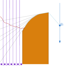
Observe that the edges of trace the trajectories of vertices of . We distinguish two types of vertices in , red vertices and blue vertices. The red vertices are either polygon vertices, or endpoints of extension segments for which contains at least one other polygon vertex. All other vertices –these correspond to endpoints of extension segments such that – are blue. This coloring of the vertices of also induces a coloring of the edges of . See Fig. 6. Since all red vertices have fixed locations, the corresponding red edges in are horizontal line segments. Furthermore, observe that every polygon edge is visible from in a single time interval. Hence, there are at most two moving endpoints per polygon edge. This implies that every horizontal strip defined by two consecutive red edges contains at most two blue edges.
As moves, the extension segment rotates around , and thus the point moves monotonically along the boundary of . That is, traces a -monotone curve through (i.e. any line parallel to the -axis or -axis intersects it in at most a single connected region). It follows that the total number of intersections with the red edges is . We further split each horizontal strip (defined by the red edges of ) at vertices of the curve traced by . Since this curve has complexity , the total number of strips remains . Each such strip is (still) crossed by at most two blue edges. The edges in the trajectory of as well as those blue edges are curves of constant algebraic degree. Hence a pair of such curves intersect only times, and thus every strip contributes at most a constant number of intersections. Since we have strips, we thus also get at most intersections. The lemma follows. ∎
Lemma 7.
The bisector is involved in at most -collapse events.
Proof.
Fix a vertex , and consider the endpoint of . By Lemma 6 this point intersects at most regions of and throughout the motion of and . It then follows that there are time intervals during which the distances and are both continuous and constant algebraic degree. We restrict the domains of and to the time intervals during which is closer to than . It follows that and still consist of pieces.
Now observe that any -collapse event of on corresponds to a time where: is closer to than , and the endpoint of is equidistant to and , that is, . Hence, the number of such events equals the number of intersections between (the graphs of) and . Since and both consist of pieces, each of constant algebraic degree, the number of intersections, and thus the number of -collapse events on is . Similarly, the number of events on is . The lemma follows by summing these events over all vertices . ∎
Lemma 8.
The bisector is involved in at most -collapse events.
Proof.
We observe that in a -collapse of edge of both and must be on extension segments and in the shortest path map of or at time . Hence a -collapse occurs at the intersection point of and . In particular, at such an event, the distances from to and from to are equal.
If and both occur in a single shortest path map, say , this -collapse event corresponds to an event at which the combinatorial structure of changes. Thus, the total number of such changes is at most (Lemma 2). We thus focus on the case that is an extension segment in and is an extension segment in .
Since the combinatorial structure of and changes at most times, the total number of pairs of extension segments that we have to consider is . We now argue that for each such pair there are at most times where , and thus there are at most -collapse events involving the pair . The total number of -collapse events is then as claimed.
The distance function from to is a piecewise hyperbolic function with pieces. The same is true for the distance function from to . We then consider maximal time intervals during which both these distance functions are continuous, and during which and are part of their respective shortest path maps. There are at most such intervals. Since and move along a trajectory of constant complexity (i.e. they either rotate continuously around and , respectively, or remain static), the distance function from via to a point on also consists of pieces, each of constant algebraic degree. The same applies for the distance function , for on . Therefore, during each time interval, the distance functions from to and from to are also continuous low-degree algebraic functions. Such functions intersect at most times, and thus the number of -collapse events in every interval is at most constant. Since we have intervals, the number of -collapses involving and is . ∎
Theorem 9.
Let and be two points moving linearly inside . The combinatorial structure of the bisector of and can change times. This bound is tight in the worst case.
Proof.
The combinatorial structure of the bisector changes either at a vertex event, a -collapse, or a -collapse. By Lemmas 5, 7, and 8 there are at most most , , and , such events respectively. We can use symmetric arguments to bound the expand events. Thus the structure of changes at most times. By Lemma 4 this bound is tight in the worst case. ∎
Even though the (combinatorial structure of the) entire bisector may change times in total, the trajectories of its intersection points with the boundary of have complexity at most :
Lemma 10.
The trajectory of has edges, each of which is a constant degree algebraic curve.
Proof.
The trajectory of changes only at vertex events or at -collapse events. By Lemmas 5 and 7 the number of such events is at most . Fix a time interval in between two consecutive events, and assume without loss of generality that moves on an edge of that coincides with the -axis. We thus have , for some function . Since we have that , for some quadratic functions and and constants , and . By repeated squaring and basic algebraic manipulations it follows that is some constant degree algebraic function in . Hence, every edge in the trajectory of corresponds to a constant degree algebraic curve. ∎
3.2 A Kinetic Data Structure to Maintain a Bisector
We first describe a simple, yet naive, KDS to maintain that is not responsive and then show how to improve it to obtain a responsive KDS.
3.2.1 A Non-Responsive KDS to Maintain a Bisector
Our naive KDS for maintaining stores: (i) the extended shortest path maps of and using the data structure of Aronov et al. [6], (ii) the vertices of , ordered along from to in a balanced binary search tree, and (iii) for every vertex of , the cell of and of that contains . Since all cells in and are triangles, this requires only certificates per vertex. We store these certificates in a priority queue .
At any time where changes combinatorially (i.e. at an event) the shortest path to a vertex of changes combinatorially, which indicates a change in the cells that contain . Hence, we detect all events. Conversely, when any vertex of moves to a different cell there is a combinatorial change in the bisector, so each event triggered by parts (ii) and (iii) of the KDS is an external event. The events at which or changes are internal (unless they also cause a combinatorial change in a shortest path to a vertex of ).
The events at which or changes are handled as in Aronov et al. [6]. However, such an event may cause the shortest path to several bisector vertices to change and we would need to recompute the certificates for maintaining which cell of the each bisector vertex lies in. The internal update for the takes time [6] and each certificate can be recomputed in time by computing the appropriate distance functions. Unfortunately, there may be certificates to update, which means such an event may take time. We will describe how to avoid this problem later, but we first describe how the rest of the events of the KDS are handled.
At any external event, a vertex of leaves its cell in or , and enters a new one. In all cases we delete the certificates corresponding to , and replace them by new ones. Depending on the type of event, we also update appropriately, i.e. in case of a - or -collapse event we remove a vertex from and in case of -expand events we insert a new vertex in . We describe how to handle a vertex event in more detail, as they may happen simultaneously with -collapse or expand events.
Consider a vertex event at vertex at time , at which a bisector endpoint, say , stops to intersect an edge of .
If there are no points in other than for which the shortest path to or passes through then the vertex event is easy to handle; at such an event simply moves onto the other edge incident to . In doing so, it crosses into a different cell of or . So, we update the certificates associated with and continue to the next event.
If there are points in some region for which and both pass through , then these points are now all equidistant to and , and hence at time the entire region is actually a subset of the bisector . See Fig. 4. This region is bounded by the extension segment incident to in , or the extension segment incident to in , that is, or . As a result, the endpoint will jump to either or (the other endpoint of or , respectively). Moreover, this extension segment becomes part of the bisector in the simultaneously occurring -expand event. This new vertex of moves on the other extension segment incident to . Hence, to update our KDS we insert a new vertex in the balanced binary search tree representing , create the corresponding certificates tracking in and , and we update the certificates tracking in and .
If there are points for which only one of the shortest paths to or , say , passes through , the bisector endpoint continues on the other edge incident to , while a new vertex is created on moving along . We insert in and create appropriate certificates tracking and in and like in the previous case.
Observe that we may also have vertex events at which a bisector endpoint jumps onto while it was moving on an edge not incident to before in a situation symmetric to in the second case described above. In such a case the vertex event coincides with a -collapse event in which a bisector vertex hits (and thus the boundary of its cell in and ) at . This is the reverse situation of the one depicted in Fig. 4. In this case we delete and its certificates, and update the certificates tracking .
Each external event involves only a constant number of vertices of . Furthermore, as each such vertex is involved in only a constant number of certificates. Updating a certificate can easily be done in time, as this involves a constant number of updates into the binary search tree representing and the event queue. Hence, handling an external event can be done in time.
Observe that at any moment we maintain only certificates, stored in a priority queue. We thus use space, and the updates to the priority queue require time. The total number of events for maintaining and is only , which is dominated by the events at which itself changes (Theorem 9). So our KDS is compact, and efficient, but not responsive as updates to the may require time. In the next section we show that we do not actually need to maintain these certificates explicitly.
3.2.2 A Responsive KDS to Maintain a Bisector
First we dissect in some more detail the anatomy of a bisector. Each bisector consists of two endpoints which are degree 1 vertices and a chain of degree 2 vertices connecting them. We can further divide this chain based on which parts are directly visible from the sites defining the bisector. This division results in at most 5 pieces, as illustrated in Fig. 7; some pieces may not be present in every bisector. First there is a double-visible piece that is visible from both sites and . Since is a simple polygon, this piece consists of a single line segment. Adjacent to the double-visible piece on either side there may be a single-visible piece that is only visible to or to , but not both. Lastly, there are up to two non-visible pieces that are not directly visible from either or .
We will still store the bisector vertices in a balanced binary tree ordered along the bisector, but we will store the certificates for the vertices in each piece separately.
Storing the certificates for the partially visible pieces
For each of the at most four degree 2 vertices that separate the pieces as well as the degree 1 endpoints, we store the cells of and that contain it, and track their events explicitly as before.
We observe that for internal vertices of the single-visible piece there can be no events. Each of these internal vertices lies on an extension segment of a single convex chain of vertices in the simple polygon and these extension segments do not intersect. Therefore no 2,2-collapses can occur, and hence no certificates need to be stored.
Storing the ceritificates of the non-visible pieces
The non-visible pieces are trickier, since 2,2-collapses may occur when a vertex moving on an extension segment of moves to a different cell of . Fortunately such potential events on a single non-visible bisector piece are related and form a strict ordering, regardless of the exact distance functions of the various vertices to and .
We define event points to be the locations at which 2,2-collapses that may occur. Consider two degree 2 vertices and that are internal to a non-visible piece of bisector between sites and , such that and are adjacent on the bisector and we have that is on an extension segment of and is on an extension segment of . Let the event point denote the intersection between these two extension segments. A 2,2-event between and corresponds to the event point being on the bisector between and . Without loss of generality assume that the event point currently lies in the Voronoi cell of . We can then use the certificate to detect the 2,2-event between and . As we saw above maintaining these certificates explicitly is not efficient as any change in the shortest path towards or requires us to recompute the failure time. Therefore, we will maintain two balanced binary search trees: one with all event points that lie in the Voronoi cell of (ordered along the bisector), and one with all event points that lie in the Voronoi cell of . We will augment the balanced binary search trees so that each node stores some additional information. In particular, a node in the tree storing the events in the Voronoi cell of stores: an event point (in order along the bisector), (ii) the event point in its sub tree that will be on the bisector first, and three fields: an event value, a maximum event value, and two offsets (one for each child) that will help maintain this event point that will be on the bisector first. We will describe these in more detail later. This way, we end up with a structure similar to a kinetic tournament [8]. Therefore, we can then compute an explicit failure time only for the two event points stored in the roots of the trees.
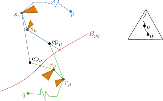
For a single non-visible bisector piece between sites and , Consider event points and where is a child of in the tree. Let and denote the first polygon vertex on the shortest path from towards and respectively and let and be defined symmetrically. See Fig. 8. Then we can rewrite the certificate for as
and the certificate for similarly. Then observe that if and , then will be on the bisector before if and only if . Hence, we use as the event value of node . This creates a strict ordering of the event values, and thus of the event points in the Voronoi cell of . Unfortunately in many cases the first vertex on the path towards or will not be the same for every vertex on the bisector. Therefore we introduce an offset value to allow comparing event points that have different first vertices on their paths towards and .
If and , we should compare based on a common vertex on the paths towards and , which may be any combination of or and or . As these cases are analogous, we consider the case where and are on the shortest paths towards and respectively for both event points. (Intuitively and are further towards and .)
Now the values we would like to compare are
However these are not what the event values store. With some rewriting, we find that the above inequality holds if and only if
We call the offset of with respect to . In the other three cases we get a similar definition of offset. Now each node will store the maximum event value in its subtree as follows.
For a leaf the maximum is its own event value, i.e. . For an internal node, it is the maximum over its own event value and the maximum values of its children with their offsets with respect to added. The event point that realizes this maximum event value is then the first event point in the subtree of that will be on the bisector. Hence, the maximum event value the root can then be used to determine the first time an -event happens among the bisector vertices stored in the tree.
Note that the above data structure stores only a constant number of certificates directly involving or , all of which are stored at the root of the tree. Therefore, we can efficiently support changes in the movement of and . Let be a polygon vertex that is on the shortest paths from to all the bisector vertices stored in the tree (note that such a vertex exists, as the bisector vertices are all part of a single non-visible piece of the bisector). When the shortest path from to changes, we only have to update the offset stored at the root of the tree. Recomputing this offset may take time, and so does updating the certificates of the root in the global event queue.
Furthermore, we can support splitting the tree, and therefore this invisible-piece of the bisector, at a vertex in time, since a split affects nodes in the balanced binary search tree, and recomputing the offsets (and the corresponding maximum event values) takes time per node. Similarly, we can handle joining two invisible-pieces of bisector in time as well. This then also means we can insert or delete individual bisector vertices in time.
Handling Events
We now replace part (iii) of the naive structure with the data structure described above. As argued, we are still guaranteed to detect all events. However, we can now handle them in time, rather than time. When changes, as becomes collinear with the first two polygon vertices and on a shortest path to , we can now update the certificates in each of the pieces efficiently. When the anatomy of the bisector changes, this may involve joining or splitting two of the invisible pieces. Thus, this takes time. Updating the certificates within in each piece can also be done in time as argued before. Similarly, handling the other bisector events can be done in time. We therefore obtain the following theorem:
Theorem 11.
Let and be two sites moving linearly inside a simple polygon with vertices. There is a KDS that maintains the bisector that uses space and processes at most events, each of which can be handled in time. Additionally it can support movement changes of and in time and splitting the bisector at any given vertex in time.
4 A Voronoi Center

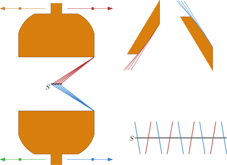
Let be the point equidistant to , , and if it exists. Note that Aronov et al. [5] proved that if it exists, it is unique (Lemma 2.5.3). We refer to as the Voronoi center of , , and . Note that there may be times at which does not exist, and thus the trajectory of may be disconnected. We identify five types of events at which may appear or disappear, or at which the movement of can change (see Fig. 9). They are:
-
•
-collapse events in which collides with the boundary of the polygon (in a bisector endpoint) and disappears from ,
-
•
-expand events in which appears on the boundary of as two bisector endpoints intersect, creating a point equidistant to all three sites,
-
•
vertex-events where appears or disappears strictly inside , as two sites, say and , are equidistant to a vertex that appears on the shortest paths to ,
-
•
-collapse events where one of the geodesics from either , , or to loses a vertex,
-
•
-expand events where one of the shortest paths gains a new vertex.
Observe that, as the name suggests, at a -collapse event the Voronoi center (a degree 3 vertex in ) disappears as it collides with the endpoint of a bisector (a degree 1 vertex). Similarly, at a -collapse event a degree 2 vertex on one of the bisectors disappears as it collides with a degree 3 vertex (the Voronoi center ). As in case of the bisector, some of these events may coincide. In the next section, we bound the number of events, and thus the complexity of the trajectory of . We then present a kinetic data structure to maintain in Section 4.2.
4.1 Bounding the Number of Events
We give a construction in which the trajectory of has complexity , and then prove a matching upper bound.
Lemma 12.
The trajectory of the Voronoi center of three points , , and , each moving linearly, may have complexity .
Proof.
The main idea is that we can construct a trajectory for of complexity , even when two of the three sites, say and , are static. We place and so that their bisector , a piecewise hyperbolic curve of complexity , intersects an (almost) horizontal line times. We can realize this using two convex chains and in similar to Lemma 4. See Fig. 10 for an illustration. We now construct a third convex chain in and place the third site so that the extension segments in incident to the vertices of all lie very close to . Thus, each such segment intersects times. We choose the initial distances so that the voronoi center lies on the rightmost segment of . Now observe that as moves away from , the center will move to the left on , and thus it will pass over all intersection points of with the extension segments of the vertices in . At each such time, the structure of one of the shortest paths , , or changes (they gain or lose a vertex from , , or , respectively). Hence, the trajectory of changes times.
Next, we argue that we can make “swing” from left to right times by having and move as well. The Voronoi center will then encounter every intersection point on times. It follows that the complexity of the trajectory of is as claimed.
The idea is to add two additional convex chains, and , that make the bisector between and “zigzag” times throughout the movement of and . We can achieve this using a similar construction as in Lemma 4. To make sure that the bisector between and remains static, we create a third chain , which is a mirrored copy of , and we make move along a trajectory identical to that of . See Fig. 10. Finally, observe that , and thus will indeed encounter all intersection points on times. The lemma follows. ∎
Lemma 13.
The number of -collapse events is at most .
Proof.
At a -event to exits the polygon. Observe that at such a time a pair of bisector endpoints, say and , intersect. By Lemma 10 the trajectories of and have edges, each of which is a constant degree algebraic curve. Thus, there are time intervals during which both and move along the boundary of , and their movement is described by a constant degree algebraic function. So such a time interval, and coincide only times. It follows that the total number of -collapse events involving , , and is . ∎
Lemma 14.
The number of vertex events is at most .
Proof.
Fix a vertex and a pair of sites . By Lemma 3 the site among closest to can change at most times. Therefore, can produce at most vertex events due to the pair . Summing over all vertices and all pairs gives us an bound. ∎
Theorem 15.
The trajectory of the Voronoi center has complexity . Each edge is a constant degree algebraic curve.
Proof.
A vertex in the trajectory of corresponds to either a -collapse or expand, a vertex event, or a -collapse or expand. By Lemma 13 the number of -collapse events, and symmetrically, the number of -expand events, is . By Lemma 14 the number of vertex events is also . We now bound the number of -collapse (and symmetrically -expand) events by . Each such an event corresponds to a breakpoint in the distance function between and one of the three sites. Hence, at such a time , leaves an (extended) shortest path map cell in one of the three shortest path maps, say , and enters a neighboring cell of . Let and be the extended shortest path map cells in and containing , respectively.
All cells in the (extended) shortest path map of are triangles, and the map changes only times throughout the movement of (Lemma 2). Hence, corresponds to a constant complexity region in whose boundaries are formed by constant degree algebraic surfaces, and there are such regions in total. Similarly, we have choices for the constant complexity regions and corresponding to and . Observe that within , all points have the same combinatorial shortest paths to , , and , and thus the distance functions are continuous hyperbolic functions. Given these distance functions, the trajectory of is a constant degree algebraic curve. Such a curve can intersect the boundary of at most times. It follows that the maximum complexity of is thus . ∎
4.2 A Kinetic Data Structure to Maintain a Voronoi Center
Our KDS for maintaining stores: (i) the extended shortest path maps of , , and , (ii) the cells of these shortest path maps containing (when lies inside ), and (iii) the endpoints of all bisectors (for all pairs), and their cyclic order on . In particular, for each such endpoint we keep track of the cells of and that contain it. See Fig. 11 for an illustration. At any time we maintain certificates, which we store in a global priority queue.
Observe that at -collapse, -collapse, and -expand events the shortest path from to one of the sites changes combinatorially. Hence, we can successfully detect all such events. At a vertex event a vertex is equidistant to two sites, say and . At such a time, one of the two endpoints of leaves an edge of , and thus exits a shortest path map cell in (and ). Since we explicitly track all bisector endpoints, we can thus detect this vertex event of . Finally, at every -expand event two such bisector endpoints collide, and thus change their cyclic order along . We detect such events due to certificates of type (iii).
Any time at which changes cells in a shortest path map results in a combinatorial change of its movement. Hence, any failure of a certificate of type (ii) is an external event (a -collapse, -collapse, or -expand). The certificates of types (i) and (iii) may be internal or external.
Theorem 16.
Let and be three sites moving linearly inside a simple polygon with vertices. There is a KDS that maintains the Voronoi center that uses space and processes at most events, each of which can be handled in time. Updates to the movement of , , and , can be handled in time.
Proof.
Certificate failures of type (i) are handled exactly as described by Aronov et al. [6]. This takes time (by again implementing the dynamic convex hull queries using the Brodal and Jakob structure [9]). Note that changes to the shortest path maps may affect the certificates that guarantee that or a bisector endpoint lies in a particular SPM cell. In these cases we trigger a type (ii) or type (iii) certificate failure. At a certificate failure of type (ii) at which exits a shortest path map cell, we remove all certificates of type (ii) from the event queue. Next, for each site , , and , we compute the new cell in the shortest path map containing (if still lies inside ). Finally, we create the appropriate new type (ii) certificates. Since all cells have constant complexity, the total number of certificates affected is also . Computing them can be done in time, e.g. by re-querying the shortest path maps.
Certificate failures of type (iii) where the movement of a bisector endpoint changes are handled using the same approach as in Section 3.2. Furthermore, at such an event we check if appears or disappears, that is, if the event is actually a vertex event of . In this case, we recompute in time [25]. If disappears then we delete all type (ii) certificates. If appears then we locate the cell of , of , and of that contains , and insert new type (ii) certificates that certify this. Finding the cells and updating the certificates can be done in time. At a certificate failure of type (iii) where two bisector endpoints collide, we check if the intersection point is equidistant to all three sites, and is thus a -expand event. Similarly to the approach described above, we add new type (ii) certificates in time in this case.
Maintaining the extended shortest path maps requires handling events [6]. Events where crosses a boundary of an extended SPM correspond to changes in the trajectory of . By Theorem 15 there are at most such events. This dominates the events that we have to handle to maintain the bisector endpoints in cyclic order around (Lemmas 10 and 13).
In addition to , , and , we maintain only a constant amount of extra information. Since the KDS to maintain such a shortest path map is local and supports changing the movement of in time, the same applies for our data structure as well. We therefore obtain a compact, responsive, local, and efficient KDS. ∎
5 The Geodesic Voronoi Diagram
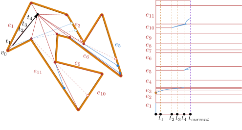
In this section we consider maintaining the geodesic Voronoi diagram as the sites in move. As a result of the sites in moving, the Voronoi vertices and edges in will also move. However, we observe that all events involving Voronoi edges involve their endpoints; two edges cannot start to intersect in their interior as this would split a Voronoi region, see Fig. 12(a). Similarly, the interior of a Voronoi edge cannot start to intersect the polygon boundary. This means we can distinguish the following types of events that change the combinatorial structure of the Voronoi diagram.

-
•
Edge collapses, at which an edge between vertices and shrinks to length zero. Let , with , be the degrees of and , respectively. We then have a -collapse.
-
•
Edge expands. These are symmetric to edge collapses.
-
•
Vertex events, where a degree 1 vertex of crosses over a polygon vertex.
Indeed, we have seen most of these events when maintaining an individual bisector or Voronoi center (a degree 3 vertex in ). The only new types of events are the -collapse and -expand events which involve two degree 3 vertices. They are depicted in Fig. 12.(b). We again note that some of these events may happen simultaneously.
Theorem 17.
Let be a set of sites moving linearly inside a simple polygon with vertices. During the movement of the sites in , the combinatorial structure of the geodesic Voronoi diagram changes at most times. In particular, the events at which changes, and the number of such events, are listed in Table 1.
We prove these bounds in Section 5.1. For most of the lower bounds we generalize the constructions from Sections 3 and 4. For the upper bounds we typically fix a site or vertex (or both), and map the remaining sites to a set of functions in which we are interested in the lower envelope. In Section 5.2 we develop a kinetic data structure to maintain .
5.1 Bounding the Number of Events
We analyze the number of collapse events and the number of vertex events. The expand events are symmetric to the collapse events.
5.1.1 1,2-collapse Events
Lemma 18.
There may be -collapse events.
Proof.
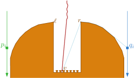
We construct a polygon with a “pit” and two chains and of reflex vertices, and we place “-shaped” obstacles at the bottom of the pit. See Fig. 13. We make the sites move downwards in pairs . All sites have the same speed, and they are spaced sufficiently far apart so that sites of different pairs do not interfere with each other. Site moves down left of the pit, so that for a sufficiently large time the shortest path from to the “-shaped” obstacles in the pit goes via . Symmetrically, moves downwards on the right side of the pit. As in Lemma 4 we make the chains and so that the bisector between and moves from left to right over the obstacles in the pit times. Now consider the ray from the left endpoint of the top right chain through the top-left vertex of a -shaped obstacle. Let be the point where this ray hits the floor of the pit. The site closest to changes times from to (as the endpoint of the bisector sweeps from right to left). Every such a time corresponds to a -collapse event. Since we have pairs, the lemma follows. ∎
Lemma 19.
The number of -collapse events is at most .
Proof.
Any -collapse event in the Voronoi diagram uniquely corresponds to a -collapse event of a bisector for some sites . By Lemma 7 the number of -collapse events in is . The lemma follows by summing over all pairs . ∎
5.1.2 1,3-collapse Events
Lemma 20.
There may be -collapse events.
Proof.
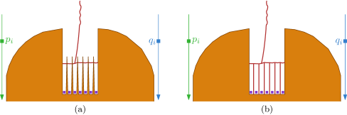
We use a similar construction with a “pit” and pairs of entities as in Lemma 18. See Fig. 14(a). Place spikes at the bottom of the pit and place a site between them. As two sites and move down, their bisector sweeps over all spikes causing the voronoi center of , and the site between the spikes as the bisector to hit the side of each spike, causing a -collapse event each time. Since the upper convex chains of the polygon consist of vertices, every pair of vertices causes such events. Note that while the horizontal part of the bisectors between the spikes moves up as a pair of vertices moves down, it “resets” when a new pair arrives, thus this process can be repeated times using new sites each time and the lemma follows. ∎
By Lemma 13 any triple , , generates at most -collapse events. So, summing over all triples this immediately gives us an upper bound. Next, we argue that we can also bound the number of -collapses by , for some .
Lemma 21.
The number of -collapse events is at most .
Proof.
Fix a site and an edge of the polygon. We now bound the number of -collapse events on site involving site by , for some constant . Since we have sites and edges, the lemma then follows. At any time , the Voronoi region of intersects in at most a single connected interval [1]. All -events on involving occur on one of the two endpoints of this interval. Let be the endpoint such that lies right of the edge of that starts in . See Fig. 15. Next, we bound the number of events occurring at . Bounding the number of events occurring at the other endpoints is analogous.
Observe that is a bisector endpoint for some site . More specifically, it is the “lowest” such endpoint along . At an -collapse event, the site that defines this “lowest” endpoint changes, that is, two bisector endpoints and meet. More formally, let and let be the value such that for all points . For a site we then define the function
If now follows that a -collapse event at corresponds to a vertex in the lower envelope . Since the trajectory of any has complexity whose edges are low-degree algebraic curves (Lemma 10) that pairwise intersect times, the same applies for function . It follows that their lower envelope has complexity , for some constant [31], and thus the number of -collapses at is at most as well. ∎
Corollary 22.
The number of -collapse events is at most
.
5.1.3 2,2-collapse Events
Lemma 23.
There may be -collapse events.
Proof.
We use the construction from Lemma 4 in which the bisector of a single pair of sites changes times. We now simply create such pairs that all move along the same trajectories. We choose the starting positions such that the distance between two consecutive points and ( and ) is very large, so that for each pair the bisector appears in the Voronoi diagram at the time when and pass by our construction. ∎
Lemma 24.
The number of -collapse events is at most .
Proof.
Fix two vertices and . By Lemma 3 there are a total of maximal time intervals during which both and have unique closest sites, and the distances from and to their respective closest sites, say and , is a continuous hyperbolic function. Consider such an interval , and observe that during , there is only a single extension segment in the (non extended) , and thus in , incident to . Similarly, there is a single extension segment in incident to . Like in Lemma 8, we now have that in the distances from and to the intersection point of and are both continuous algebraic functions of constant degree. These functions intersect only a constant number of times, and thus there are at most -collapse events per interval. In total we thus have events per pair, and events in total. ∎
5.1.4 2,3-collapse Events
Lemma 25.
There may be -collapse-events.
Proof.
We give two constructions. The first one gives -collapse events and the second one . The lemma then follows.
For the first construction we modify the construction in Fig. 10 slightly. The main idea is that each time the Voronoi center moves into a new cell defined by , , and a -collapse event occurs. Thus for three sites, we get such events. When we repeat this process by moving triples along the trajectories of , , and , the first part of the lower bound follows. In order to do this, we modify the polygon by adding two horizontal rectangles, one to the left of and one to the left of , and a vertical rectangle, above . These rectangles contain (the trajectories of) the future triples. By making the convex chains , , and steep enough, we can ensure that all events occur close enough together, limiting how long the horizontal rectangles need to be. Thereby, we can make sure they do not overlap the vertical path of . Alternatively, we can make the part of the polygon containing horizontal, and use the “zigzags” between and and between and to adapt the length of the paths appropriately.
The second construction is sketched in Fig. 16. We again have an obstacle with a convex chain of complexity . On the left side of this obstacle, we have fixed sites. The bisectors of adjacent sites and the lines extending the edges of the convex chain form a grid of complexity . On the right side of the obstacle, we drop a site such that the bisector of and the fixed sites sweeps over the entire grid, causing 2,3-collapse events. By dropping sites sufficiently far apart, we can repeat this process times, leading to the second part of the lower bound. ∎
Consider an extension segment of incident to and let be some linear parameter along such that is a point along . Let denote the distance function from a site to .
Lemma 26.
Consider a time interval in which has fixed combinatorial structure. The function restricted to this interval is a bivariate piecewise constant degree algebraic function of complexity .
Proof.
Every cell of has constant complexity. Moreover, the function describing the movement of has constant complexity as well. In particular, this function consists of at most three pieces, in at most one of which lies on the (rotating) line through and , and in the other two has a fixed location. It follows that each cell contributes constant complexity to . Since there are only cells, the total complexity of is at most . Every patch of represents the Euclidean distance of a fixed point (a polygon vertex) to a points on a line rotating through . This can be described by a constant degree algebraic function. ∎
Lemma 27.
The number of -collapse events is at most .
Proof.
Any -collapse event at some time occurs on an extension segment incident to a polygon vertex . In particular, is an extension segment of the shortest path map of the site which is closest to at time . Furthermore, by Lemma 1, has only one such an extension segment at any time. We can thus charge the -event to . We now bound the number of such charges to a vertex by . The lemma then follows.
Split time into time intervals in which: (i) the site closest to is fixed, and the distance from to is a continuous hyperbolic function, and (ii) the shortest path maps from all sites have a fixed combinatorial structure. It follows from Lemmas 2 and 3 that there are intervals in total.

Fix such a time interval . For any (other) site , let be the intersection point of and the bisector of and . See Fig. 17. The distance function restricted to has complexity (Lemma 26), and the distance from to has constant complexity. It follows that the complexity of the trajectory of in the interval is also . In turn, this implies that the function has only breakpoints in interval . Moreover, each piece of is some constant degree algebraic function. For and we let be undefined.
Since we have intervals, it follows that the function has a total complexity of .
Any -collapse charged to now corresponds to a vertex on the lower envelope of the functions : at such a vertex two sites, say and are both closest to , and there is no other site closer. The lower envelope has complexity . It follows that there are thus also at most -collapse events charged to . The lemma follows. ∎
5.1.5 3,3-collapse Events
Lemma 28.
There may be -collapse events.
Proof.
See Fig. 14(b). As in Lemma 20, we again we drop points in pairs, but now the bottom of the pit contains collinear sites . As the bisector between and moves from left to right, it crosses the vertical bisector between and , collapsing an edge of the Voronoi diagram. Since both and are degree 3 vertices, this is a -collapse. It follows that every pair of sites , , generates such events. The lemma follows. ∎
Lemma 29.
There may be -collapse events.
Proof.
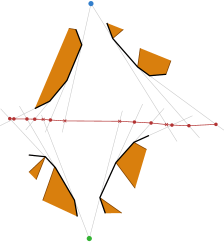
The construction uses ideas similar to the “wine-glass” construction from Fig. 5. We will describe the construction in two steps as there are two different scale levels involved. The main construction is shown in Fig. 18, where we have two mirrored wine-glasses where the top of the wineglasses are right angles. If we assume the wineglasses and the four moving points are perfectly mirrored (we will add tiny deviations later) it follows that the four points are continuously co-circular with the centerpoint moving on a horizontal line in the middle between the two wine-glasses. By tailoring the slopes of the edges along the curved parts of the wine-glasses we can ensure that the centerpoint moves left to right along a horizontal line segment times. We denote this line segment by .
Next we add some variation to the two wineglasses. We replace the two right angled corners on the right with two convex chains with the following properties; (i) the lines aligned with the edges of the chain intersect the line segment , (ii) the intersection points on alternate between lines aligned to edges of the upper chain and of the lower chain, and (iii) when moving from left to right along the nearest among the right two sites alternates. Note that for (iii) we will only consider the motion of the sites vertically above and below the wineglasses, so this statement does not depend on the exact location of the sites during the motion.
The bound on the number of 3,3-collapse events can then be shown from these properties. First observe that the bisector between the two left sites is still a horizontal line and the portion of it that appears in the Voronoi diagram ends in a Voronoi vertex on . As we can make the modification to the wineglasses arbitrarily small, the main motion of the bisector between the two upper (or the two lower) sites still remains the same. That is, it still sweeps from left to right along . It follows that the Voronoi vertex that is the end of the bisectors of the two left sites also sweeps from left to right on . By property (iii) the nearest among the two right sites alternates times, which means that they are equidistant times. So with each sweep of , there are points where all four sites are equidistant and it follows that there are different 3,3-collapse events.
We repeat the process with quadruples of points. Note that all events of a quadruple happen in some time interval. We make the wine glasses sufficiently wide so that these time intervals are disjoint, and so that the sites of quadruples that already have had their events are sufficiently far away from the center of the construction (segment ) that they do not interfere with later quadruples. Hence, each of the quadruples of points create events, resulting in the claimed bound. ∎
Next, we prove an upper bound for the number of -collapse events. We use the same general idea as Guibas et al. [16] use for sites moving in under semi-algebraic motion.
Consider the bisector of a pair of points , and orient it so that a point on is above a point on the bisector if the pseudo-triangle defined by has those points in that clockwise order on its boundary, see Fig. 19.
Lemma 30.
Let be a geodesic disk containing , , and on its boundary in that order, let be a disk with , and in that order on the boundary. The center of lies “below” the center of in the order along if and only if contains .
Proof.
To show that lies inside , we argue that . Consider the geodesic triangle defined by , , and . The distance function from to points on is convex [29], and thus has its maximum at or . So, if lies inside , it now readily follows that .
If lies outside then we claim that the shortest path must intersect . The geodesic triangle splits into three pieces: itself, a part “above” containing the points in so that the geodesic triangle is oriented clockwise, and the remaining part “below” the . See Figure 19 for an illustration. Since lies on the boundary of in between and (with respect to a clockwise order), and it does not lie inside , it must lie above . Since lies “below” (in the order along ), it must lie below or inside the triangle. Finally, since is contained in , it must thus intersect .
Assume, without loss of generality that intersects in a point . We then obtain by triangle inequality that:
We thus obtain that
where the second equality follows from the fact that and are on the boundary of . This implies that , which in turn gives us that
Hence, we obtain that and thus lies inside . ∎
Lemma 31.
There are -collapse events.
Proof.
The main idea is as follows. Recall that a degree three Voronoi vertex is defined by three sites, that lie on the boundary of a geodesic disk that is empty of other sites. At a -collapse event at time two degree three Voronoi vertices and collide, and hence their empty geodesic disks coincide. Relabel the sites so that at the time of the event, the clockwise order of the points along the boundary of this disk is . We will charge the collapse event to the pair , and argue that each such pair is charged at most times. Therefore the total number of -collapse events is at most as claimed.
To bound the number of times each pair is charged, we map each other site to a function , and argue that -collapse events charged to correspond to vertices of the lower envelope of these functions. What remains is to describe these functions.
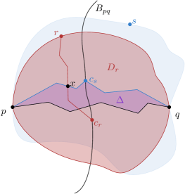
For any site , consider the geodesic disk with , , and on its boundary that has as its centerpoint. At any time there is at most one such a disk [26, 27]. Observe that (if the center point lies inside ) it lies on the bisector , and that the points divide the boundary of into two parts. Let denote the boundary section which is clockwise adjacent to and the part that is counterclockwise adjacent to , see Fig. 20. The site can be on either boundary part. Let be the set of sites , so that is on (it may not be inside for all sites ) and is on . Now observe that any -collapse event at time charged to will have .
Consider two sites , and their centers and . By Lemma 30, point lies below on the bisector if and only if the disk contains .
At a -event charged to , the disks and are both empty of other sites. Hence, it follows that their centers and are the “lowest” centers among all sites in . Our final step is to formally capture this notion of lowest definition of , and argue about its complexity.
Let denote the midpoint of the shortest path between and (and observe that lies on ). Then for a point on the bisector that is above , we define . For a point below , we define . Then for any site not equal to or , we define
For any point , there are time intervals in which the movement of the Voronoi center , and the (lengths of the) shortest paths between the sites , , and defining are described by a constant degree algebraic function (Theorem 15). For each such a time interval can cross and thus enter or leave at most times. Hence, the complexity of is also . Since we are considering sites we are interested in the lower envelope of functions, each consisting of pieces of constant algebraic complexity. Therefore the number of changes in the lower envelope, and thus the number of events charged to is bounded by [31]. This completes the proof. ∎
5.1.6 Vertex Events
Lemma 32.
There may be vertex events.
Proof.
We once more use a similar approach as in Lemma 20. We build the “pit” construction shown in Fig. 13 and we drop the sites in pairs of two, say pairs . The left and right convex chains have complexity and are built such that the endpoint of the bisector of and sweeps the “T-shaped” obstacles every time its geodesic path to or changes. It now follows that the point where the bisector of and hits the bottom of the pit moves across the obstacles in the pit times. Thus the number of vertex events is . ∎
Lemma 33.
The number of vertex events is at most .
Proof.
Directly from Lemma 3, summing over all vertices. ∎
5.2 A KDS for a Voronoi Diagram
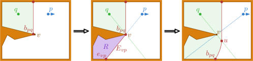
In this section we develop a KDS to maintain the Voronoi diagram of . Our KDS essentially stores for each site the extended shortest path map of its Voronoi cell, and a collection of certificates that together guarantee that the shortest paths from the sites to all Voronoi vertices remain the same (and thus the KDS correctly represents ). The main difficulties that we need to deal with are shown in Fig. 21. Here, becomes the site closest to vertex , and as a result a part of the polygon moves from the Voronoi cell of to the Voronoi cell of . Our KDS should therefore support transplanting this region from the SPM representation of into and vice versa. Moreover, part of the bisector becomes a bisector , which means that any certificates internal to the bisector (such as those needed to detect 2,2-events) change from being dependent on the movement of to being dependent on the movement of . Next, we show how to solve the first problem, transplanting part of the shortest path map. Our KDS for the bisector from Theorem 11 essentially solves the second problem. All that then remains is to describe how to handle each event.
Maintaining Partial Shortest Path Maps
To support transplanting a part of into we extend the data structure of Aronov et al. [6]. Observe that is a tree rooted at , and we transplant only subtrees, rooted at some polygon vertex . Our representation of should support: (i) link operations in which we add the subtree rooted at as a child of , (ii) cut operations in which we cut an edge , (iii) shortest path queries in which we report the length of the shortest path from some vertex to the root , and (iv) principal-child queries in which we report the principal child of some non-root node . The principal child is the child of for which the angle between and , where is the parent of , is minimal. We need this operation to support updating the certificates of 333Since the root is the only node storing a moving point, all certificates involve only nodes from the first three layers of the tree. Hence, it suffices to compute the principal child only for direct children of the root.. To support these operations, we store twice: once in a link-cut tree [32] and once in an Euler tour tree [17]. Both these structures support link and cut operations in time. The link-cut trees support query operations on node-to-root paths, and hence we use them to answer shortest path queries in time (plus time to report the actual path, if desired). The Euler tour trees support query operations on subtrees, and hence we use them to answer principal child queries. In particular, we maintain the children of in cyclic order around , starting with . This way link and cut operations still take time, and the principal child of can be reported in constant time.
The data structure
The full KDS thus consists of an extended shortest path map for every Voronoi cell maintained as described above; and certificates for each degree three vertex, degree one vertex, and each bisector. For every degree three vertex we maintain the cells of , and that contain it and its distance to neighboring vertices. For every degree one vertex , we store the cells of and that contain it, which edge of it is on, and if applicable its separation from neighboring degree one vertices on the same edge. For each bisector, we store the data structure of Theorem 11. Our data structure uses a total of space.
It is not to difficult to see that this certificate structure captures all external events. For collapse and expand events involving degree three vertices we explicitly certify that the distance to its adjacent vertices is non-zero. For events involving degree one vertices we explicitly track which edge contains each such a vertex. This allows us to detect vertex events. Furthermore, we maintain distance of each degree one vertex to other degree one vertices on the same edge. Thus we can detect 1,3-expand events. We also maintain which cells of the the vertex is contained in, which allows us to detect 1,2-expand and -collapse events. What remains are the 2,2-events. These are detected by the data structure of Theorem 11.
Handling events
Handling the events is similar to what we described in Sections 3.2 and 4.2. Hence, we describe only what is new or different here.
At all external-events we have to update the shortest path map representations of the Voronoi cells. In most cases, this involves adding or removing a single vertex to the shortest path map. This can easily be handled using local computations in time. The most expensive operation is computing the location of a new Voronoi vertex, which may take time [25]. In case of vertex events, we may have to move an entire region in to . Since all shortest paths in such a region go via the vertex involved, we can perform these updates in time using the above data structure.
Since there are now sites, we maintain certificates, and thus updating the event queue takes time. Furthermore, we now have multiple degree three vertices, and thus we have to handle -collapse and expand events. These are handled in a similar fashion to the other events; we update the Voronoi regions, and compute new certificates certifying the movement of the vertices involved from scratch. All these updates can be done in time.
At a vertex event where and are equidistant to a vertex , the region that moves from to may now be bounded by a bisector rather than (see Fig. 21). Since, at the time of the event, the relevant parts of and coincide we can obtain the new part of by splitting , and updating the movement of the associated sites. In particular, replacing the function expressing the distance to by the distance from to . Our bisector KDS allows such updates in time (Theorem 11).
Finally, we may have to update the certificates associated with the Voronoi vertices as a result of changes to the individual shortest path maps. For example, when a site can no longer see polygon vertex , this affects all Voronoi certificates of vertices for which the shortest path goes through . While our KDS for the bisector (Theorem 11) can update the affected certificates of such a change efficiently, this unfortunately does not hold for the certificates associated with degree one or degree three vertices. Updating these requires time, where is the number of neighbors of in . It is an interesting open question to try and handle such events implicitly as well. We therefore obtain the following result:
Theorem 34.
Let be a set of sites moving linearly inside a simple polygon with vertices. There is a KDS that maintains the geodesic Voronoi diagram that uses space and processes at most events, each of which can be handled in time, where is the number of neighbors of the affected Voronoi cell.
6 Refining the bounds
For simplicity, the bounds in this paper have been expressed as a function of (the number of sites) and (the number of vertices of ). When dealing with simple polygons, it is common to use an additional parameter: the number of reflex vertices of (denoted by ). Since each reflex vertex is in particular a vertex, we immediately have , but in general the two parameters are asymptotically different.
We believe that most terms that appear in our bounds can be turned into a function of instead. This can be achieved by looking at each of the bounds and carefully analyzing what depends on and what actually depends on . Alternatively, we can use the polygon simplification technique of Aichholzer et al. [3]:
Theorem 35 (Theorem 1 of [3], rephrased).
Given a simple polygon of vertices and reflex vertices, there exists a simple polygon of vertices such that any shortest path in is a shortest path in .
This result is a general tool that can be used to transform many dependencies of into dependencies of . Note that the focus of [3] is algorithmic (i.e., they study at how fast can be computed) whereas our proof is combinatorial. For our purposes, Aichholzer’s result implies that bisectors in must be contained in the bisectors of . Thus, we can track topological changes of bisectors in by focusing on instead (and since has vertices, the bounds on the number of such events would depend on ).
This method can be used for most events but not all of them: for example, vertex events happen when a bisector sweeps through any vertex of (and thus the dependency on cannot be removed). Thus we wonder if there is some technique similar to Aichholzer’s that we could use to refine all of our bounds and that we can obtain the correct dependency in and . We leave this as an interesting open question for future work.
7 Conclusion
We constructed compact, responsive, local, and efficient kinetic data structures for maintaining bisectors and Voronoi centers of a geodesic Voronoi diagram. These data structures use linear space and process a worst-case optimal number of events. The bisector KDS handles each event in time, while the Voronoi center needs time per event. Together, these data structures form a compact KDS for maintaining the full augmented geodesic Voronoi diagram. For each type of event we provide upper bounds of the worst-case number of events (which ranges from cubic to fifth power). These bounds are close to the truth, since for each case we provide an instance whose number of events is tight or almost tight to the corresponding theoretical upper bound.
Obvious follow up questions are: to design a more efficient KDS for this problem, refine the bounds (for example by using the number of reflex vertices of the polygon), or to close the gaps between the worst-case upper and lower bounds. A more interesting variation of the latter problem would be to find more realistic instances; our constructions are rather degenerate in that the polygons contain narrow corridors that all sites pass through at controlled speeds, causing many changes to the diagram. It would be interesting to define a notion of realistic or natural input and study the number of events in such situations. Such realistic input assumptions have proven to be useful in related problems, for example when analyzing the complexity of the area visible to a point on a terrain [11].
There are two other ways in which our research can be extended. First, in the type of movement: in this paper we focused on sites that move linearly, but more general patterns could be considered. For example, can one design a compact, responsive, local, and efficient KDS for more general algebraic motions of bounded degree ? If so, what are the worst-case number of events that could happen (as a function of )?
Another way to extend this would be to consider more general domains. Instead of a simple polygon one could look into polygonal domains (i.e., polygons with holes). Although many results extend to this space, the main difference when holes are added is that we can have paths of different homotopy connecting the same two points. Thus, any KDS that maintains the Voronoi diagram of moving sites must be able to compute which of them is the shortest one and detect when a different one becomes shorter. The result is that the complexity of most algorithms increases significantly and in some cases it is known that running times grow from linear to polynomials of degree larger than 10 [7]. As an intermediate step, one could consider adapting our results to domains with , , or more generally holes.
Acknowledgements
We would like to thank Man-Kwun Chiu and Yago Diez for interesting discussions during the initial stage of this research. We would also like to thank the anonymous reviewers which helped us significantly improve the presentation of this paper and made it more accessible to a wider audience.
References
- [1] Pankaj K. Agarwal, Lars Arge, and Frank Staals. Improved dynamic geodesic nearest neighbor searching in a simple polgyon. In Proc. 34th Annual Symposium on Computational Geometry, volume 99 of Leibniz International Proceedings in Informatics (LIPIcs), pages 4:1–4:14. Schloss Dagstuhl–Leibniz-Zentrum fuer Informatik, 2018.
- [2] Pankaj K. Agarwal, Haim Kaplan, Natan Rubin, and Micha Sharir. Kinetic Voronoi diagrams and Delaunay triangulations under polygonal distance functions. Discrete & Computational Geometry, 54(4):871–904, 2015.
- [3] Oswin Aichholzer, Thomas Hackl, Matias Korman, Alexander Pilz, and Birgit Vogtenhuber. Geodesic-preserving polygon simplification. International Journal of Computational Geometry and Applications, 24(04):307–323, 2014. Special issue of selected papers from the 24th International Symposium on Algorithms and Computation (ISAAC’13).
- [4] Boris Aronov. On the geodesic Voronoi diagram of point sites in a simple polygon. Algorithmica, 4(1):109–140, 1989.
- [5] Boris Aronov, Steven Fortune, and Gordon Wilfong. The furthest-site geodesic Voronoi diagram. Discrete & Computational Geometry, 9(3):217–255, 1993.
- [6] Boris Aronov, Leonidas J. Guibas, Marek Teichmann, and Li Zhang. Visibility queries and maintenance in simple polygons. Discrete & Computational Geometry, 27(4):461–483, 2002.
- [7] Sang Won Bae, Matias Korman, and Yoshio Okamoto. Computing the geodesic centers of a polygonal domain. Computataional Geometry: Theory and Applications, 77:3–9, 2019.
- [8] Julien Basch, Leonidas J. Guibas, and John Hershberger. Data structures for mobile data. Journal of Algorithms, 31(1):1–28, 1999.
- [9] G. S. Brodal and R. Jacob. Dynamic planar convex hull. In Proceedings of the 43rd Annual IEEE Symposium on Foundations of Computer Science, pages 617–626, 2002.
- [10] M. de Berg, O. Cheong, M. van Kreveld, and M. Overmars. Computational Geometry: Algorithms and Applications. Springer, Berlin, 3rd edition, 2008.
- [11] Mark de Berg, A. Frank van der Stappen, Jules Vleugels, and Matthew J. Katz. Realistic input models for geometric algorithms. Algorithmica, 34(1):81–97, 2002.
- [12] Erik D. Demaine, Joseph S. B. Mitchell, and Joseph O’Rourke. The open problems project. http://maven.smith.edu/~orourke/TOPP/.
- [13] Herbert Edelsbrunner and Ernst P. Mücke. Simulation of simplicity: A technique to cope with degenerate cases in geometric algorithms. ACM Transactions on Graphics, 9(1):66–104, 1990.
- [14] J. E. Goodman and J. O’Rourke. Handbook of Discrete and Computational Geometry. CRC Press series on discrete mathematics and its applications. Chapman & Hall/CRC, 2004.
- [15] Leonidas Guibas, John Hershberger, Daniel Leven, Micha Sharir, and Robert E. Tarjan. Linear-time algorithms for visibility and shortest path problems inside triangulated simple polygons. Algorithmica, 2(1):209–233, 1987.
- [16] Leonidas J. Guibas, Joseph S. B. Mitchell, and Thomas Roos. Voronoi diagrams of moving points in the plane. In Graph-Theoretic Concepts in Computer Science, pages 113–125, Berlin, Heidelberg, 1992. Springer.
- [17] Monika R. Henzinger and Valerie King. Randomized fully dynamic graph algorithms with polylogarithmic time per operation. Journal of the ACM, 46(4):502–516, 1999.
- [18] John Hershberger and Subhash Suri. An optimal algorithm for Euclidean shortest paths in the plane. SIAM Journal on Computing, 28(6):2215–2256, 1999.
- [19] Menelaos I. Karavelas and Leonidas J. Guibas. Static and kinetic geometric spanners with applications. In Proceedings of the Twelfth Annual ACM-SIAM Symposium on Discrete Algorithms, SODA ’01, pages 168–176, 2001.
- [20] Chih-Hung Liu. A nearly optimal algorithm for the geodesic Voronoi diagram of points in a simple polygon. In 34th International Symposium on Computational Geometry (SoCG 2018), volume 99 of Leibniz International Proceedings in Informatics (LIPIcs), pages 58:1–58:14, Dagstuhl, Germany, 2018. Schloss Dagstuhl–Leibniz-Zentrum fuer Informatik.
- [21] Anna Lubiw, Jack Snoeyink, and Hamideh Vosoughpour. Visibility graphs, dismantlability, and the cops and robbers game. Computataional Geometry: Theory and Applications, 66:14 – 27, 2017.
- [22] J. S. B. Mitchell. Shortest paths among obstacles in the plane. In Proceedings of the 9th Annual ACM Symposium on Computational Geometry, pages 308–317, 1993.
- [23] Joseph S. B. Mitchell. A new algorithm for shortest paths among obstacles in the plane. Annals of Mathematics and Artificial Intelligence, 3(1):83–105, 1991.
- [24] Eunjin Oh. Optimal algorithm for geodesic nearest-point Voronoi diagrams in simple polygons. In Proceedings of the Thirtieth Annual ACM-SIAM Symposium on Discrete Algorithms, pages 391–409. SIAM, 2019.
- [25] Eunjin Oh and Hee-Kap Ahn. Voronoi diagrams for a moderate-sized point-set in a simple polygon. Discrete & Computational Geometry, 2019.
- [26] Eunjin Oh, Sang Won Bae, and Hee-Kap Ahn. Computing a geodesic two-center of points in a simple polygon. Computataional Geometry: Theory and Applications, 82:45 – 59, 2019.
- [27] Eunjin Oh, Jean-Lou De Carufel, and Hee-Kap Ahn. The geodesic 2-center problem in a simple polygon. Computataional Geometry, 74:21–37, 2018.
- [28] Evanthia Papadopoulou and Der-Tsai Lee. A new approach for the geodesic Voronoi diagram of points in a simple polygon and other restricted polygonal domains. Algorithmica, 20(4):319–352, 1998.
- [29] Richard Pollack, Micha Sharir, and Günter Rote. Computing the geodesic center of a simple polygon. Discrete & Computataional Geometry, 4:611–626, 1989.
- [30] Natan Rubin. On kinetic Delaunay triangulations: A near-quadratic bound for unit speed motions. Journal of the ACM, 62(3):25:1–25:85, 2015.
- [31] Micha Sharir and Pankaj K Agarwal. Davenport-Schinzel sequences and their geometric applications. Cambridge university press, 1995.
- [32] Daniel D. Sleator and Robert Endre Tarjan. A data structure for dynamic trees. Journal of Computer and System Sciences, 26(3):362 – 391, 1983.
- [33] Subhash Suri. A linear time algorithm with minimum link paths inside a simple polygon. Computer Vision, Graphics and Image Processing, 35(1):99–110, 1986.