Single-electron quantum dynamics in high-harmonic generation spectrum from LiH molecule: analysis of potential energy surfaces for electrons constructed from a model of localized Gaussian wave packets with valence-bond spin-coupling

Abstract

High-harmonic generation (HHG) spectrum from a LiH molecule induced by an intense laser pulse is computed and analyzed with potential energy surfaces for electron motion (ePES) constructed from a model of localized electron wave packets (EWP) with valence-bond spin-coupling. The molecule has two valence ePES with binding energies of 0.39 hartree and 1.1 hartree. The HHG spectrum from an electron dynamics on the weaker bound valence ePES, virtually assigned to Li 2s, exhibits a dominant peak at the first harmonic without plateau and cut-off. This compares with the free electron spectrum under oscillating laser field and is comprehensive with the shape and depth of the ePES. The other valence ePES, assingned to H 1s, is deeper bound such that the overall profile of the wave function is well approximated by a Gaussian of the width comparable to the Li-H bond length. However, a small fraction, less than $10^{-3}$, of the probability density amplitude tunnels out from the bound potential with high wave number, and spreads over tens of nm’s with parts recombining to the molecule due to the laser field oscillation. This minor portion of the electronic wave function is the major origin of the HHG extending up to 50 harmonic orders. Nonlinear dynamics within the potential well induced by the laser field oscillation also contributes to the HHG up to 30 harmonic orders.

I Introduction

Study of electron dynamics in materials is an active field of research reinforced by recent advances of attosecond time-resolved laser spectroscopy Bucksbaum (2007); Kling and Vrakking (2008); Krausz and Ivanov (2009); Ramasesha et al. (2016). Electron dynamics induced by intense and short laser pulse generates high harmonics of the input light Krause et al. (1992); Schafer et al. (1993); Corkum (1993); Baggesen and Madsen (2011); Bandrauk et al. (2013); Itatani et al. (2004); Haessler et al. (2011); Salières et al. (2012); Offenbacher et al. (2015); Ghimire et al. (2010); Yoshikawa et al. (2017). Proper analysis of the high-harmonic generation (HHG) spectrum is expected to provide keys to understanding time-dependent behavior of electrons in materials. Current standard picture is the three-step model Corkum (1993) where half-ionized electrons driven by oscillating laser field recombine to the molecule and emit light. This process is expected to self-probe the molecular electronic states via the so-called molecular orbital tomography Itatani et al. (2004); Haessler et al. (2011); Salières et al. (2012); Offenbacher et al. (2015). The three-step model has been generalized to the momentum space for solid states Vampa et al. (2014).

Computational modeling of electron dynamics in atoms and molecules cannot be a trivial extension of conventional molecular orbital or density functional methods. Ordinary atomic orbital basis functions are insufficient to describe spatially large amplitude motion of electrons induced by intense laser fields. Use of plane wave basis functions will require many functions up to high wave numbers to describe both local atomic and non-local ionized states. Treating many electrons will add further complexities where adequacy of the mean-field orbital picture is not obvious. Consequently, computational studies of electron dynamics under strong field on realistic molecular models are rather scarce (although the reference list herein Grossmann (2013); Geppert et al. (2008); Takemoto and Becker (2011); Löstedt et al. (2012); Telnov et al. (2013); Tolstikhin et al. (2013); Li et al. (2016); Sato and Ishikawa (2013, 2015); Remacle et al. (2007); Nest et al. (2008); Remacle and Levine (2011); Nikodem et al. (2017); Balzer et al. (2010); Ulusoy and Nest (2012) is not exhaustive). The size of the molecules that have been treated so far is also limited.

In previous publications Ando (2017, 2018), we demonstrated that a model of floating and breathing localized electron wave packets (EWP) with non-orthogonal valence-bond (VB) spin-coupling Ando (2009, 2012); Hyeon-Deuk and Ando (2014a, b, 2015, 2016); Ando (2016) can be used to construct potential energy surfaces for single electron motion (ePES) as functions of the EWP positions. In Ref. Ando (2018), the method was applied to a LiH molecule under short and intense laser pulse. It was found that a sum of the HHG spectra from single electron dynamics on two valence ePES, that were virtually assigned to Li 2s and H 1s, agree well with that from the time-dependent complete-active-space (TD-CASSCF) calculation Sato and Ishikawa (2013, 2015). In this work, we continue the analysis with further details of the wave functions to clarify the origin and mechanism of the HHG spectrum.

Section II outlines the theory and computation. The analysis of electron wave function dynamics is presented in Sec. III. Section IV concludes.

II Model and Computation

The theory and computation for the ePES with the VB EWP model and for ther HHG spectra induced by an intense laser pulse are mostly identical to those described in our previous publication Ando (2018). We thus outline here the essential part, with further details summarized in Appendix.

In the VB EWP model, the total electronic wave function is represented by a form of an antisymmetrized product of spatial and spin functions. The spatial part is modeled by a product of one-electron functions of a spherical Gaussian form with variable central position $\boldsymbol{q}_{i}$ and width $\rho_{i}$,

$$\phi_{i}(\boldsymbol{r})=(2\pi\rho_{i}^{2})^{-3/4}\exp(-|\boldsymbol{r}-\boldsymbol{q}_{i}|^{2}/4\rho_{i}^{2}).$$ (1)

The spin part is composed of a single configuration of the perfect-pairing form. The electronic energy $E$ is computed as a function of the variables $\{\boldsymbol{q}_{i}\}$ and $\{\rho_{i}\}$ at a given nuclear geometry $\{\boldsymbol{R}_{I}\}$. Their optimal values $\{\boldsymbol{q}_{i}^{(0)}\}$ and $\{\rho_{i}^{(0)}\}$ are determined by minimizing the energy $E$. The ePES for the $j$-th electron ${\cal V}_{j}(\boldsymbol{q})$ is constructed by fixing the variables other than $\boldsymbol{q}_{j}$ as

$${\cal V}_{j}(\boldsymbol{q})=E(\boldsymbol{q}_{1}^{(0)},\cdots,\boldsymbol{q}_{j-1}^{(0)},\boldsymbol{q},\boldsymbol{q}_{j+1}^{(0)},\cdots,\boldsymbol{q}_{N}^{(0)},$$

$$\rho_{1}^{(0)},\cdots,\rho_{N}^{(0)};\{\boldsymbol{R}_{I}\}).$$ (2)

The time-dependent Schrödinger equation for an electron on the ePES ${\cal V}_{j}(\boldsymbol{q})$ was solved numerically. (Note that this is not the evolution of the localized EWP of Eq. (1). The EWP are used only for the construction of ePES.)

The scheme was applied to a LiH molecule under an intense laser pulse. The electron dynamics in LiH has been studied in many previous works Sato and Ishikawa (2013, 2015); Remacle et al. (2007); Nest et al. (2008); Remacle and Levine (2011); Nikodem et al. (2017); Balzer et al. (2010); Ulusoy and Nest (2012) as a prototype of simple heteronuclear molecules with two core and two valence electrons. The accuracy of the VB EWP model for the ground and excited electronic states of LiH has been examined in Ref. Ando (2016). The static electron correlation was well described by the VB model, and the ionic Li⁺H^- character in the ground state was reproduced by the floating and breathing degrees of freedom of the EWP. (See the insets of Figs. 4 and 6.)

To construct the potential curves ${\cal V}_{j}(\boldsymbol{q})$, the EWP centers $\boldsymbol{q}_{j}$ that were assigned to Li 2s and H 1s from their optimal position and width were displaced along the bond direction on the $x$-axis in the laboratory frame. The Li nucleus was at the origin and the H nucleus was at $x=+2.3$ bohr Sato and Ishikawa (2015). For comparison, we carried out calculations of a free electron under the same laser pulse. We also computed WP dynamics with semiclassical approximation, where the WP widths were fixed at the optimal values $\{\rho_{i}^{(0)}\}$ and the classical equations of motion for the WP center $\boldsymbol{q}_{j}$ on ${\cal V}_{j}(\boldsymbol{q})$ were solved.

In what follows, the terms ‘Li 2s electron’ and ‘H 1s electron’ are used for notional convenience, but they differ from the ordinary atomic orbitals clamped at the nuclear centers. Rather, they are evolving on the ePES assigned to Li 2s and H 1s from their initial size and position. (They may be called instead ‘weaker bound’ and ‘stronger bound’ valence electrons.) The initial condition for the electronic wave function at $t=0$ was the form of Eq. (1) with the center $\boldsymbol{q}_{j}^{(0)}$ and width $\rho_{j}^{(0)}$ optimized in the ground state without the external field: $x^{(0)}_{1}=2.11$ bohr and $\rho^{(0)}_{1}=1.75$ bohr for the Li 2s electron and $x^{(0)}_{2}=2.16$ bohr and $\rho^{(0)}_{2}=0.77$ bohr for the H 1s electron. (See the insets of Figs. 4 and 6.)

III Results and Discussion

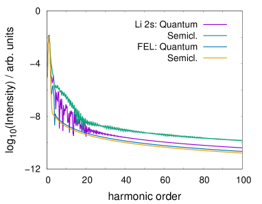
Figure 1: High-harmonic generation spectra from an electron on the valence electronic potential energy curve assigned virtually to Li 2s, computed with full quantum and semiclassical methods, compared with those from a free electron (FEL).

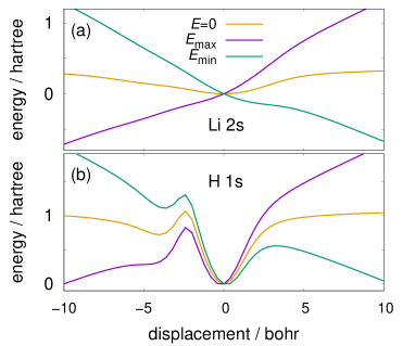
Figure 2: Potential energy curves ${\cal V}_{j}(x-x^{(0)}_{j})$ for the valence electrons virtually assigned to Li 2s and H 1s, at times when the laser field intensity is zero, maximum, and minimum.

We first analyze the dynamics of Li 2s electron. Figure 1 displays the HHG spectrum from the quantum and semiclassical calculations. The spectra from a free electron under the same laser field are also included. All spectra exhibit a dominant peak at the first harmonic. For the free electron, it is a simple consequence of the WP motion that directly follows the laser-field oscillation. Similarly, the dominance of the first harmonic in the Li 2s spectrum is comprehended to come from a free-electron-like motion due to the shallowness of the ePES displayed in Fig. 2(a), with a small binding energy of 0.39 hartree.

Figure 3 displays the trajectories of the position displacement expectation value. Similarity between the Li 2s electron and free electron is seen. The amplitude of motion of the H 1s electron is much smaller, which implies weak correlation between the Li 2s and H 1s electrons. The trajectory of the H 1s electron will be examined later with Figs. 8 and 9.

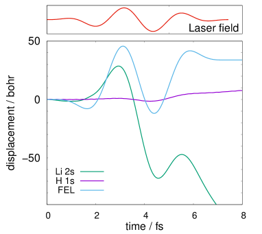
Figure 3: Trajectories of the position displacement expectation value for electrons on the valence electronic potential energy curves assigned virtually to Li 2s and H 1s and for a free electron (FEL). The top panel displays the time profile of the electric field intensity of the laser pulse.

The probability density of the Li 2s wave function is plotted in Fig. 4 at $t=0$ and times when the laser field intensity was the maximum ($t=3.2$ fs), minimum ($t=4.3$ fs), and at the end of laser pulse ($t=7.5$ fs). (The laser pulse shape is shown in Fig. 3.) In a few femtoseconds, the wave function broadens to the width of 100 bohr without developing notorious peak structure. At the end of laser pulse, the wave function acquires a complex structure. This would be the origin of the weak peaks up to $\sim$20 harmonic orders in Fig. 1.

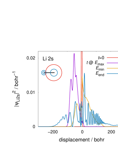
Figure 4: Probability density of an electron on the valence electronic potential energy curve assigned virtually to Li 2s, at times when the laser field intensity is maximum, minimum, and at the end of the laser pulse. The abscissa is the displacement from the EWP center at $t=0$. The inset at the upper-left displays circles of radius $\rho^{(0)}_{i}$, the wave packet widths optimized at zero field, with the electron wave packet assinged to Li 2s in red, and the Li and H nuclei at the left and right ends of the thick black horizontal line.

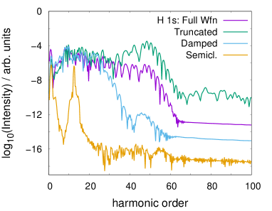
Figure 5: High-harmonic generation spectra from an electron on the valence electronic potential energy curve assigned virtually to H 1s, computed with full quantum, truncated, and damped wave functions and with semiclassical approximation.

Figures 5 and 6 are the corresponding analysis for the H 1s electron. The ePES for H 1s electron displayed in Fig. 2(b), has the binding energy of $\sim$1.1 hartree, which is large enough to keep the binding well structure under the modulation by the laser field. Consequently, as seen in Fig. 6, the wave packet maintains the Gaussian-like shape and width. This seemed to imply that the semiclassical description would be appropriate. However, as seen in Fig. 5, the semiclassical calculation was unable to reproduce the plateau and cut-off of the HHG spectrum.

Figure 6: Probability density of an electron on the valence electronic potential energy curve assigned virtually to H 1s, at times when the laser field intensity is maximum, minimum, and at the end of the laser pulse. The abscissa is the displacement from the EWP center at $t=0$. The inset at the upper-left displays circles of radius $\rho^{(0)}_{i}$, the wave packet widths optimized at zero field, with the electron wave packet assinged to H 1s in red, and the Li and H nuclei at the left and right ends of the thick black horizontal line.

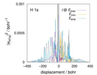
Figure 7: Same as Fig. 6 but in different scales of the axes to see part of the probability densities, about $10^{-3}$ times smaller in amplitude and $10^{2}$ times broader in spatial range.

The puzzle was resolved by looking into fine details of the wave function. Figure 7 displays the same probability densities as those in Fig. 6 but in different scales of the axes, about $10^{-3}$ times smaller amplitude and $10^{2}$ times broader spatial range. These portions of the wave function were created via tunneling through the potential barriers at both sides of the ePES in Fig. 2(b). They appear to carry the high frequency components. This is confirmed by computing the spectra with truncated and damped wave functions. The spectrum with the truncated wave function was computed by limiting the spatial range of integration when computing the dipole moment by

$$\mu(t)=-e\int_{x_{\rm min}}^{x_{\rm max}}x|\psi(x,t)|^{2}dx,$$ (3)

that is, the wave function $\psi$ was computed normally but the dipole moment was computed from the limited part of the wave function near the molecule. We set $x_{\rm min}=-2.4$ bohr and $x_{\rm max}=+3.2$ bohr to include the main part of the WP in Fig. 6. The spectrum with the damped wave function was computed with the absorbing potential Gonzalez-Lezana et al. (2004) placed at $x=\pm 13$ bohr such that once a part of the wave function tunnels out of the potential well, it is damped out. The difference between the truncated and damped calculations is that the tunneled portion may return to the molecular region in the former but not in the latter. As seen in the spectra in Fig. 5, the damped calculation gives the plateau up to $\sim$30 harmonic orders, but the higher region between 30 and 50 harmonic orders is suppressed. For the truncated wave function, the spectrum around 50 harmonic orders is rather enhanced.

The picture offered by this analysis is that the small portion of wave function that leaked out from the molecular binding potential via tunneling carries high frequency components to yield the HHG between 30 and 50 harmonic orders. The HHG up to 30 harmonic orders also come from the nonlinear dynamics within the unharmonic potential modulated by the laser field.

The binding energy of 1.1 hartree for the H 1s electron is consistent with the well-known formula for the cut-off energy of HHG spectra Krause et al. (1992),

$$E_{c}=I_{p}+3.17U_{p}$$ (4)

where $I_{p}$ is the ionization potential and $U_{p}$ is the ponderomotive energy. The present parameters for the laser pulse (see Appendix) gives $U_{p}=0.77$ hartree. With $I_{p}=1.1$ hartree for the H 1s electron (Fig. 2(b)), Eq. (4) gives the cut-off energy of 58 harmonic orders, consistent with the result in Fig. 5. With the binding energy of 0.39 hartree for the Li 2s electron, the same calculation gives 47 harmonic orders, though the plateau and cut-off is not seen in Fig. 1 due to the free-electron-like dynamics as discussed above.

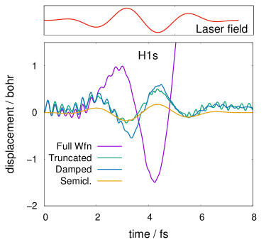
Figure 8: Trajectories of the position displacement expectation value for an electron on the valence electronic potential energy curve assigned virtually to H 1s, computed with full quantum, truncated, and damped wave functions and with semiclassical approximation.

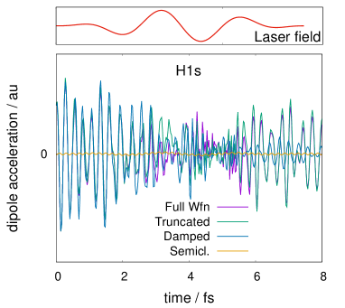
Figure 9: Trajectories of the dipole acceleration for an electron on the valence electronic potential energy curve assigned virtually to H 1s, computed with full quantum, truncated, and damped wave functions and with semiclassical approximation.

Figure 8 displays the trajectory of the position displacement expectation value for the H 1s electron. In $t<2$ fs, the quantum, truncated, and damped calculations agree well. After 2 fs, when the laser field passed the minimum, the latter two start to deviate. The quantum result is reasonable as the electron is accelerated opposite to the field direction. Although the tunneled portion has small amplitude, it contributes to the position expectation with large spatial range. The truncated and damped results are from the remainder of the wave function. The semiclassical trajectory basically follows the laser field but with smaller amplitude. The corresponding trajectories of the dipole acceleration are displayed in Fig. 9, in which the oscillations are seen clearer. The period of the prominently seen oscillation is $\sim$0.3 fs compared to 2.5 fs of the laser light. The difference among the methods is small in the short time, but becomes more apparent in the longer time, particularly for the damped wave function.

IV Concluding Remarks

The origin of the HHG spectrum from a LiH molecule has been analyzed. The electron dynamics on the weaker bound valence ePES is the main origin of the first harmonic but not of the higher harmonics. In view of the spatially large amplitude oscillation of the electron (Fig. 3), the three-step model seemed to apply. However, the analysis indicated that the ePES the electron is shallow such that the electron dynamics is rather similar to that of a free electron under the oscillating laser field. By contrast, the ePES for the other valence electron is deep enough to hold the major part of the wave function such that the oscillation amplitude under the laser field is as small as the molecular size, which implies that the ionization in normal sense does not occur. Rather, small portion of the wave function that leaked out of the potential well via tunneling was the main origin of the HHG up to 50 harmonic orders. Nonlinear dynamics within the potential well induced by the laser field oscillation was another source of HHG up to 30 harmonic orders.

We note that the Li-H bond length of 2.3 bohr is shorter than the experimental value of 3.2 bohr Orth and Stwalley (1979). The former was taken from Ref. Sato and Ishikawa (2015) which employed the soft-Coulomb potential and found the equilibrium bond length at 2.3 bohr. By contrast, our model gives 3.1 bohr Ando (2012). It would be thus intriguing to examine the effect of bond compression and extension with our model. In particular, the small hump of ePES on the negative side of the displacement in Fig. 2 (b) is due to the Li nucleus, so the tunneling through the barrier will be affected by the bond length. Another related issue would be inclusion of nuclear motion. In the present framework, an approximate treatment with nuclear wave packets would be possible Hyeon-Deuk and Ando (2014a, b, 2015, 2016). These are open for future examinations.

Appendix

Here we summarize the details of theory and computation. See Ref.Ando (2018) for additional information.

The electronic wave function has a form of an antisymmetrized product of spatial and spin functions

$$\Psi(1,\cdots,N)={\cal A}[\Phi(\boldsymbol{r}_{1},\cdots,\boldsymbol{r}_{N})\Theta(1,\cdots,N)]$$

with the spatial part modeled by a product of one-electron functions

$$\Phi(\boldsymbol{r}_{1},\cdots,\boldsymbol{r}_{N})=\phi_{1}(\boldsymbol{r}_{1})\cdots\phi_{N}(\boldsymbol{r}_{N}).$$

The form of $\phi_{i}(\boldsymbol{r})$ employed in this work is given in Eq. (1). For the spin part, we employ a single configuration of the perfect-pairing form

$$\Theta=\theta(1,2)\theta(3,4)\cdots\theta(N-1,N)$$

in which $\theta(i,j)=(\alpha(i)\beta(j)-\beta(i)\alpha(j))/\sqrt{2}$.

The time-dependent electric field of the laser pulse has a form

$${\cal E}(t)={\cal E}_{0}\sin(\omega_{0}t)\sin^{2}(\pi t/\tau)\quad(0\leq t\leq\tau)$$

in the direction parallel to the Li-H bond. The frequency $\omega_{0}$ corresponds to the wavelength 750 nm. The duration $\tau$ is for three optical cycles, $\tau=3(2\pi/\omega_{0})\simeq$ 7.51 fs. The field intensity is ${\cal E}_{0}=5.5\times 10^{8}$ V/cm which corresponds to the laser intensity of $4.0\times 10^{14}$ W/cm². These parameter values were taken from Ref. Sato and Ishikawa (2015). The positive value of ${\cal E}$ corresponds to the electric field in the direction from Li to H nuclei.

The length of the simulation box was taken to be 1200 bohr, with the transmission-free absorbing potential Gonzalez-Lezana et al. (2004) of 120 bohr length at both ends. The wave functions were propagated with the Cayley’s hybrid scheme Watanabe and Tsukada (2000) with the spatial grid length of 0.2 bohr and the time-step of 0.01 au ($\sim$0.24 as). The norm of the wave function stayed unity with the deviation less than 10^-7 throughout the simulation. The semiclassical calculation was by the frozen Gaussian method with the fixed width $\rho_{j}^{(0)}$. The derivatives of the potentials ${\cal V}_{j}(\boldsymbol{q})$ were computed by the spline interpolation. The HHG spectra were computed from the Fourier transform of the dipole acceleration dynamics.

References

- Bucksbaum (2007) P. H. Bucksbaum, Science 317, 766 (2007).
- Kling and Vrakking (2008) M. F. Kling and M. J. J. Vrakking, Ann. Rev. Phys. Chem. 59, 463 (2008).
- Krausz and Ivanov (2009) F. Krausz and M. Ivanov, Rev. Mod. Phys. 81, 163 (2009).
- Ramasesha et al. (2016) K. Ramasesha, S. R. Leone, and D. M. Neumark, Ann. Rev. Phys. Chem. 67, 41 (2016).
- Krause et al. (1992) J. L. Krause, K. J. Schafer, and K. C. Kulander, Phys. Rev. Lett. 68, 3535 (1992).
- Schafer et al. (1993) K. J. Schafer, B. Yang, L. F. DiMauro, and K. C. Kulander, Phys. Rev. Lett. 70, 1599 (1993).
- Corkum (1993) P. B. Corkum, Phys. Rev. Lett. 71, 1994 (1993).
- Baggesen and Madsen (2011) J. C. Baggesen and L. B. Madsen, J. Phys. B: At. Mol. Opt. Phys. 44, 115601 (2011).
- Bandrauk et al. (2013) A. D. Bandrauk, F. Fillion-Gourdeau, and E. Lorin, J. Phys. B: At. Mol. Opt. Phys. 46, 153001 (2013).
- Itatani et al. (2004) J. Itatani, J. Levesque, D. Zeldler, H. Niikura, H. Pépin, J. C. Kleffer, P. B. Corkum, and D. M. Villeneuve, Nature 432, 867 (2004).
- Haessler et al. (2011) S. Haessler, J. Caillat, and P. Salières, J. Phys. B: At. Mol. Opt. Phys. 44, 203001 (2011).
- Salières et al. (2012) P. Salières, A. Maquet, S. Haessler, J. Caillat, and R. Taïeb, Rep. Prog. Phys. 75, 062401 (2012).
- Offenbacher et al. (2015) H. Offenbacher, D. Lüftner, T. Ules, E. M. Reinisch, G. Koller, P. Puschnig, and M. G. Ramsey, J. Electron. Spectrosc. Relat. Phenom 204, 92 (2015).
- Ghimire et al. (2010) S. Ghimire, A. D. DiChiara, E. Sistrunk, P. Agostini, L. F. DiMauro, and D. A. Reis, Nat. Phys. 7, 138 (2010).
- Yoshikawa et al. (2017) N. Yoshikawa, T. Tamaya, and K. Tanaka, Science 356, 736 (2017).
- Vampa et al. (2014) G. Vampa, C. R. McDonald, G. Orlando, D. D. Klug, P. B. Corkum, and T. Brabec, Phys. Rev. Lett. 113, 073901 (2014).
- Grossmann (2013) F. Grossmann, Theoretical Femtosecond Physics: Atoms and Molecules in Strong Laser Fields (Springer, Heidelberg, 2013).
- Geppert et al. (2008) D. Geppert, P. von den Hoff, and R. de Vibie-Riedle, J. Phys. B: At. Mol. Opt. Phys. 41, 074006 (2008).
- Takemoto and Becker (2011) N. Takemoto and A. Becker, Phys. Rev. A 84, 023401 (2011).
- Löstedt et al. (2012) E. Löstedt, T. Kato, and K. Yamanouchi, Phys. Rev. A 85, 053410 (2012).
- Telnov et al. (2013) D. A. Telnov, K. E. Sosnova, E. Rozenbaum, and S. I. Chu, Phys. Rev. A 87, 053406 (2013).
- Tolstikhin et al. (2013) O. I. Tolstikhin, H. J. Wörner, and T. Morishita, Phys. Rev. A 87, 041401(R) (2013).
- Li et al. (2016) P. C. Li, Y. L. Sheu, H. Z. Jooya, X. X. Zhou, and S. I. Chu, Sci. Rep. 6, 32763 (2016).
- Sato and Ishikawa (2013) T. Sato and K. L. Ishikawa, Phys. Rev. A 88, 023402 (2013).
- Sato and Ishikawa (2015) T. Sato and K. L. Ishikawa, Phys. Rev. A 91, 023417 (2015).
- Remacle et al. (2007) F. Remacle, M. Nest, and R. D. Levine, Phys. Rev. Lett. 99, 183902 (2007).
- Nest et al. (2008) M. Nest, F. Remacle, and R. D. Levine, New. J. Phys. 10, 025109 (2008).
- Remacle and Levine (2011) F. Remacle and R. D. Levine, Phys. Rev. A 83, 013411 (2011).
- Nikodem et al. (2017) A. Nikodem, R. D. Levine, and F. Remacle, Phys. Rev. A 95, 053404 (2017).
- Balzer et al. (2010) K. Balzer, S. Bauch, and M. Bonitz, Phys. Rev. A 82, 033427 (2010).
- Ulusoy and Nest (2012) I. S. Ulusoy and M. Nest, J. Phys. Chem. A 116, 11107 (2012).
- Ando (2017) K. Ando, Comp. Theor. Chem. 1116, 159 (2017).
- Ando (2018) K. Ando, J. Chem. Phys. 148, 094305 (2018).
- Ando (2009) K. Ando, Bull. Chem. Soc. Jpn. 82, 975 (2009).
- Ando (2012) K. Ando, Chem. Phys. Lett. 523, 134 (2012).
- Hyeon-Deuk and Ando (2014a) K. Hyeon-Deuk and K. Ando, J. Chem. Phys. 140, 171101 (2014a).
- Hyeon-Deuk and Ando (2014b) K. Hyeon-Deuk and K. Ando, Phys. Rev. B 90, 165132 (2014b).
- Hyeon-Deuk and Ando (2015) K. Hyeon-Deuk and K. Ando, J. Chem. Phys. 144, 171102 (2015).
- Hyeon-Deuk and Ando (2016) K. Hyeon-Deuk and K. Ando, Phys. Chem. Chem. Phys. 18, 2314 (2016).
- Ando (2016) K. Ando, J. Chem. Phys. 144, 124109 (2016).
- Gonzalez-Lezana et al. (2004) T. Gonzalez-Lezana, E. J. Rackham, and D. E. Manolopoulos, J. Chem. Phys. 120, 2247 (2004).
- Orth and Stwalley (1979) F. B. Orth and W. C. Stwalley, J. Mol. Spectrosc. 76, 17 (1979).
- Watanabe and Tsukada (2000) N. Watanabe and M. Tsukada, Phys. Rev. E 62, 2914 (2000).