Momentum-resolved analysis of condensate dynamic and Higgs oscillations
in quenched superconductors with tr-ARPES

Abstract

Higgs oscillations in nonequilibrium superconductors provide an unique tool to obtain information about the underlying order parameter. Several properties like the absolute value, existence of multiple gaps and the symmetry of the order parameter can be encoded in the Higgs oscillation spectrum. Studying Higgs oscillations with time-resolved angle-resolved photoemission spectroscopy (ARPES) has the advantage over optical measurements that a momentum-resolved analysis of the condensate dynamic is possible. In this paper, we investigate the time-resolved spectral function measured in ARPES for different quench protocols. We find that analyzing amplitude oscillations of the ARPES intensity in the whole Brillouin zone allows to understand how the condensate dynamic contributes to the emerging of collective Higgs oscillations. Furthermore, by evaluating the phase of these oscillations the symmetry deformation dynamic of the condensate can be revealed, which gives insight about the ground state symmetry of the system. With such an analysis, time-resolved ARPES experiments might be used in future as a powerful tool in the field of Higgs spectroscopy.

I Introduction

Angle-resolved photoemission spectroscopy (ARPES) is a powerful method as it allows to measure the electronic structure of materials directly [1]. Combined with additional time resolution (tr-ARPES), dynamic processes of systems out of equilibrium can be studied in great detail [2]. Hereby, a pump pulse excites the system in a nonequilibrium state prior to the photoemission probe pulse, which is applied after a variable time delay to scan the dynamic of the system.

In recent years, there was an evolving interest in studying collective excitations of materials in nonequilibrium as these can provide fundamental insights into the internal symmetries and properties of a system. This has been demonstrated on charge-density wave systems [3, 4, 5] and high-temperature cuprate superconductors [6, 7, 8]. In superconductors, an intrinsic collective amplitude (Higgs) mode of the order parameter exists due to spontaneous $U(1)$ symmetry breaking at the transition to the superconducting state [9, 10]. Exciting the Higgs mode is challenging and only in the last years an exploration of this area has started. This progress was heavily supported by the upcoming of new technologies like ultrafast THz spectroscopy [11], which possess the required excitation energy to not fully deplete the superconducting condensate in the pump process.

The main reason for the difficulties to excite the Higgs mode is due to the fact that the Higgs mode is a scalar mode with neither net charge nor electric dipole, which requires to go beyond the linear excitation regime. While the first predictions of the Higgs mode in superconductors are relatively old [12, 13], only indirect measurements in systems with competing charge-density wave orders could be realized in the beginning [14]. The first direct observation was performed in a THz pump-probe experiment on the $s$-wave superconductor Nb_1-xTi_xN [15], where Higgs oscillations of the order parameter, reflected in oscillations of the electromagnetic response, could be observed. Since then, only a few more experiments were reported [16, 17, 18, 19, 20], but theoretical works on the subject became more popular as it became clear that Higgs oscillations in nonequilibrium systems provide rich information about the superconducting ground state.

It was found that much information about the ground state order parameter is encoded in the Higgs oscillation frequency. First of all, the main Higgs oscillation frequency corresponds to the maximum of the absolute value of the order parameter itself [21, 22, 23, 24, 25]. In addition, multiband systems show frequencies for each band and also for the frequency of the relative phase mode (Leggett mode) [26, 27]. Excited in an asymmetric way, nontrivial gap symmetries can show additional oscillation frequencies as a result of an oscillation of the condensate in a different symmetry channel [28]. Finally, composite order parameters [29], excitations of subleading pairing channels [30] as well as coupling to other coexisting modes [20] might show up as additional frequencies.

As of now, two main approaches to study Higgs oscillations exist, namely measurements of the optical conductivity in pump-probe experiments [31, 32, 33] and resonances in third-harmonic generation in periodically driven systems [34, 35], where both methods allow to deduce the intrinsic Higgs modes. The only different approach, also in a pump-probe setup, was the prediction of Higgs oscillations in tr-ARPES [36, 37, 38], where the position of the maximum of the energy distribution curve shows oscillations with the same frequency as the Higgs mode.

In this article, we study the spectral function measured in tr-ARPES in a more general approach. While previous papers concentrated on the oscillation of spectral weight in energy, we also evaluate the amplitude oscillation, which contains more information about the condensate dynamic. We allow arbitrary gap symmetry and study the effect of quenches in symmetry channels different from the ground state. The idea behind such quenches is to model the net effect of pump pulses in a controlled way, which act on the condensate momentum-dependently. These might be realized experimentally by tuning polarization and pulse direction [28] or could be implemented in more complex approaches like transient grating [39, 40] or four-wave mixing [41] setups.

Quenching superconductors with such an approach, where the symmetry of the condensate is altered with respect to the ground state, can result in dynamically created additional Higgs modes [28]. It is important to note that we ensure that the order parameter always keeps its ground state symmetry and only the underlying condensate is modified. This is plausible as a modification of the gap symmetry and thus, the pairing interaction itself, in a conventional pump-probe experiment is unlikely. However, a modification of the condensate, i.e. the Cooper pair or quasiparticle distribution might be controllable with light excitation. In our analysis, we neglect subleading pairing channels, which may be present in some materials. A symmetry-breaking quench would activate these channels, such that Bardasis-Schrieffer modes can occur [30]. However, in many materials only a single pairing channel is dominant, such that these effects can be neglected. As we show in this work, additional Higgs mode can still occur assuming only a single pairing channel.

By evaluating the induced oscillation of the ARPES intensity, both in amplitude and weight shift in energy, we explore the creation process of these additional Higgs modes, i.e. we can understand how the dynamic of the condensate at different momenta contributes to the collective Higgs oscillation. Moreover, we compare superconductors with the same nodal gap structure but different signs, like $d$-wave and nodal $s$-wave, quenched in the same symmetry channel. A calculation of the oscillation phase in different lobes shows opposite phase oscillations, reflecting the differently induced symmetry deformations of the condensate in momentum space.

II Model and methods

II.1 Hamiltonian

We consider the mean-field BCS Hamiltonian

$$H =\sum_{{\bm{k}}\sigma}\epsilon_{{\bm{k}}}c_{{\bm{k}}\sigma}^{\dagger}c_{{\bm{k}}\sigma}-\sum_{{\bm{k}}}\left(\Delta_{{\bm{k}}}c_{{\bm{k}}\uparrow}^{\dagger}c_{-{\bm{k}}\downarrow}^{\dagger}+\mathrm{c.c.}\right)\,,$$ (1)

where $\epsilon_{\bm{k}}$ is the electron dispersion relative to the Fermi level and $c^{\dagger}_{{\bm{k}}\sigma}$, $c_{{\bm{k}}\sigma}$ the creation and annihilation operators for electrons with momentum ${\bm{k}}$ and spin $\sigma$. The momentum-dependent energy gap $\Delta_{\bm{k}}$ is defined by

$$\Delta_{{\bm{k}}} =\sum_{{\bm{k}}^{\prime}}V_{{\bm{k}}{\bm{k}}^{\prime}}\braket{c_{-{\bm{k}}^{\prime}\downarrow}c_{{\bm{k}}^{\prime}\uparrow}}\,,$$ (2)

where the pairing interaction $V_{{\bm{k}}{\bm{k}}^{\prime}}=Vf_{\bm{k}}f_{{\bm{k}}^{\prime}}$ is assumed to be separable such that we can write $\Delta_{{\bm{k}}}=\Delta f_{\bm{k}}$ with

$$\Delta=V\sum_{{\bm{k}}}f_{\bm{k}}\braket{c_{-{\bm{k}}\downarrow}c_{{\bm{k}}\uparrow}}\,.$$ (3)

Hereby, $V$ is the pairing strength and $f_{\bm{k}}$ the gap symmetry function, which can be chosen according to the symmetry groups of the underlying lattice. As we will see, tr-ARPES allows to measure the dynamic of the condensate $\braket{c_{-{\bm{k}}\downarrow}c_{{\bm{k}}\uparrow}}(t)$ by measuring the spectral function, such that we can understand how oscillations of $\braket{c_{-{\bm{k}}\downarrow}c_{{\bm{k}}\uparrow}}(t)$ at different momenta contribute to collective Higgs oscillation $\Delta(t)$.

Our results are rather independent of material parameters (see appendix E), thus, we use a quadratic dispersion $\epsilon_{\bm{k}}=tk^{2}-\epsilon_{\mathrm{F}}$ for convenience. The used numerical values of the parameters can be found in the appendix in Tab. 1. Furthermore, we restrict our calculation to two dimensions to reduce the computational costs and to correspond also to quasi-2d materials as the layered cuprates.

To calculate the induced time evolution after a quench, it is advantageous to perform a Bogoliubov transformation

$$\begin{pmatrix}\alpha_{{\bm{k}}}\\ \beta^{\dagger}_{{\bm{k}}}\end{pmatrix} =\begin{pmatrix}u_{{\bm{k}}}&-v_{{\bm{k}}}\\ v_{{\bm{k}}}&u_{{\bm{k}}}\end{pmatrix}\begin{pmatrix}c_{{\bm{k}}\uparrow}\\ c_{-{\bm{k}}\downarrow}^{\dagger}\end{pmatrix}$$ (4)

to new quasiparticle operators $\alpha_{\bm{k}}$ and $\beta_{\bm{k}}$ with

$$u_{{\bm{k}}} =\sqrt{\frac{1}{2}\left(1+\frac{\epsilon_{{\bm{k}}}}{E_{{\bm{k}}}}\right)}\,, v_{{\bm{k}}} =\sqrt{\frac{1}{2}\left(1-\frac{\epsilon_{{\bm{k}}}}{E_{{\bm{k}}}}\right)}\,.$$ (5)

In the expression above, $E_{\bm{k}}=\sqrt{\epsilon_{\bm{k}}^{2}+(\Delta f_{\bm{k}})^{2}}$ is the quasiparticle energy and we choose the phase of the equilibrium order parameter $\Delta$ to be zero. The Bogoliubov transformation is performed for this fixed value of the gap. The BCS Hamiltonian at arbitrary times for time-dependent values of the order parameter $\Delta(t)$ in Eq. (1) then reads

$$H(t) =\sum_{{\bm{k}}}R_{{\bm{k}}}(t)(\alpha_{{\bm{k}}}^{\dagger}\alpha_{{\bm{k}}}+\beta_{{\bm{k}}}^{\dagger}\beta_{{\bm{k}}})$$

$$\quad+\sum_{{\bm{k}}}C_{{\bm{k}}}(t)\alpha_{{\bm{k}}}^{\dagger}\beta_{{\bm{k}}}^{\dagger}-C_{{\bm{k}}}^{*}(t)\alpha_{{\bm{k}}}\beta_{{\bm{k}}}\,,$$ (6)

where we neglect constant terms and define

$$R_{{\bm{k}}}(t) =\frac{1}{2E_{{\bm{k}}}}\left(2\epsilon_{{\bm{k}}}^{2}+\Delta_{{\bm{k}}}(t)\Delta_{\bm{k}}^{*}+\Delta_{{\bm{k}}}^{*}(t)\Delta_{\bm{k}}\right)\,,$$ (7a)

$$C_{{\bm{k}}}(t) =\frac{1}{2E_{{\bm{k}}}}\big{(}2\epsilon_{{\bm{k}}}\Delta_{\bm{k}}-\Delta_{{\bm{k}}}(t)(E_{{\bm{k}}}+\epsilon_{{\bm{k}}})$$

$$\qquad+\Delta_{{\bm{k}}}^{*}(t)(E_{{\bm{k}}}-\epsilon_{{\bm{k}}})\big{)}\,.$$ (7b)

In equilibrium, $\Delta_{{\bm{k}}}(t)=\Delta_{\bm{k}}$ and the Hamiltonian becomes diagonal with $R_{\bm{k}}=E_{\bm{k}}$ and $C_{\bm{k}}=0$. We can express the anomalous expectation value $\braket{c_{-{\bm{k}}\downarrow}c_{{\bm{k}}\uparrow}}$ in the gap equation (3) with the new Bogoliubov quasiparticle operators and find

$$\Delta(t) =V\sum_{{\bm{k}}}f_{\bm{k}}\Big{[}u_{{\bm{k}}}v_{{\bm{k}}}\left(1-\braket{\alpha_{{\bm{k}}}^{\dagger}\alpha_{{\bm{k}}}}(t)-\braket{\beta_{{\bm{k}}}^{\dagger}\beta_{{\bm{k}}}}(t)\right)$$

$$\qquad-u_{{\bm{k}}}^{2}\braket{\alpha_{{\bm{k}}}\beta_{{\bm{k}}}}(t)-v_{{\bm{k}}}^{2}\braket{\alpha_{{\bm{k}}}^{\dagger}\beta_{{\bm{k}}}^{\dagger}}(t)\Big{]}\,.$$ (8)

II.2 Iterated equation of motion method

We calculate the time evolution of the Bogoliubov operators with the help of Heisenberg’s equation of motion

$$\partial_{t}\alpha_{{\bm{k}}}^{\dagger}(t) =\frac{\mathrm{i}}{\hbar}[\tilde{H}(t),\alpha_{{\bm{k}}}^{\dagger}(t)]\,,$$ (9a)

$$\partial_{t}\beta_{{\bm{k}}}^{\dagger}(t) =\frac{\mathrm{i}}{\hbar}[\tilde{H}(t),\beta_{{\bm{k}}}^{\dagger}(t)]\,,$$ (9b)

where the Hamiltonian $\tilde{H}(t)$, $\alpha_{{\bm{k}}}^{\dagger}(t)$ and $\beta_{{\bm{k}}}^{\dagger}(t)$ are the operators in the Heisenberg picture. To evaluate these equations, we make use of the iterated equation of motion approach [42] to write the Bogoliubov operators in the Heisenberg picture as a time-dependent superposition of the equilibrium operators

$$\alpha_{\bm{k}}^{\dagger}(t) =a_{0{\bm{k}}}(t)\alpha_{\bm{k}}^{\dagger}+a_{1{\bm{k}}}(t)\beta_{\bm{k}}\,,$$ (10a)

$$\beta_{\bm{k}}^{\dagger}(t) =b_{0{\bm{k}}}(t)\beta_{\bm{k}}^{\dagger}+b_{1{\bm{k}}}(t)\alpha_{\bm{k}}\,.$$ (10b)

Inserted into Heisenberg’s equation of motion, such an ansatz leads in general to an infinite hierarchy of equations for the prefactors $a_{i{\bm{k}}}(t)$ and $b_{i{\bm{k}}}(t)$, which have to be truncated at a certain order. However, for a bilinear Hamiltonian like the BCS Hamiltonian, the approach in Eq. (10) using only a second order ansatz for each operator is exact. This allows to derive a closed set of differential equations for the time-dependent prefactors. The derived equations are given in appendix A.

The coupled differential equations (22) are solved numerically in a self-consistent manner by evaluating the time-dependent gap equation in each time step. The initial values of the prefactors $a_{i{\bm{k}}}(0)$ and $b_{i{\bm{k}}}(0)$ are given by the initial values of the Bogoliubov quasiparticles expectation values $\braket{\alpha_{\bm{k}}^{\dagger}\alpha_{\bm{k}}}(0)$, $\braket{\beta_{\bm{k}}^{\dagger}\beta_{\bm{k}}}(0)$, $\braket{\alpha_{\bm{k}}^{\dagger}\beta_{\bm{k}}^{\dagger}}(0)$ and $\braket{\alpha_{\bm{k}}\beta_{\bm{k}}}(0)$, which themselves are determined by the electron expectation values $\braket{c_{-{\bm{k}}\downarrow}c_{{\bm{k}}\uparrow}}(0)$, $\braket{c_{{\bm{k}}\uparrow}^{\dagger}c_{-{\bm{k}}\downarrow}^{\dagger}}(0)$, $\braket{c_{{\bm{k}}\uparrow}^{\dagger}c_{{\bm{k}}\uparrow}}(0)$ and $\braket{c_{-{\bm{k}}\downarrow}c_{-{\bm{k}}\downarrow}^{\dagger}}(0)$. Depending on the type of quench, the initial values are either the equilibrium expectation values or quenched expectation values. This is described in the next section and the respective expectation values are listed in appendix A.

In order to increase the precision while keeping the numerical effort in a reasonable order, the 2d momentum space is discretized only in a small region around the Fermi level given by an energy cutoff $\epsilon_{\mathrm{c}}$. This is justified by the fact that superconductivity only occurs near the Fermi momentum $k_{\mathrm{F}}$, while contributions far away are negligible. The momentum grid was chosen in polar coordinates, with $N_{k}$ points in radial and $N_{\varphi}$ points in azimuthal direction. All the numerical values are listed in the appendix in Tab. 1.

II.3 Excitation with quantum quenches

We want to study the system in an out of equilibrium state excited by a laser pulse in an experiment. As the net effect of an ultrashort THz pump pulse is that it changes the system abruptly, we model this effect in a general manner by considering an effective quantum quench, i.e. the pump pulse acts like a quench pulse. In literature [23], the usual way to go is an interaction quench, i.e. changing the interaction strength abruptly at $t=0$ from its equilibrium value $V$ to a new value $V^{\prime}=gV$, where $g<1$, which reduces the gap $\Delta$ to a new value $\Delta(0)=g\Delta$. Then, the time evolution can be calculated starting from the equilibrium state of the old system given in Eq. (24) using the quenched gap equation with the modified pairing interaction $V^{\prime}$. The disadvantage of this method is that an interaction quench cannot easily be realized experimentally in condensed matter. Only in cold atom systems, where the interaction strength can be tuned with Feshbach resonances [43], an implementation is feasible. Besides that, an interaction quench is not directly equivalent to the effect of a quench pulse and in addition, it always acts on the whole system isotropically, whereas a momentum-dependent excitation is more interesting to study, especially for unconventional superconductors with nontrivial pairing symmetry.

Considering all of this, we implement a momentum-dependent state quench. Namely, the effect of a quench pulse is to deplete a small portion of the condensate and create a nonequilibrium quasiparticle distribution. What is happening in particular, is that the equilibrium distribution of the quasiparticles at $T=0$, e.g. the anomalous expectation value

$$\braket{c_{-{\bm{k}}\downarrow}c_{{\bm{k}}\uparrow}} =\frac{\Delta_{\bm{k}}}{2E_{\bm{k}}}\,,$$ (11)

is modified as a result of the quench pulse, where the symmetry of the quenched state $\braket{c_{-{\bm{k}}\downarrow}c_{{\bm{k}}\uparrow}}^{\prime}$ does not necessarily have to be the same as in equilibrium. To implement such a quench in a controlled way, we introduce the quenched distribution

$$\braket{c_{-{\bm{k}}\downarrow}c_{{\bm{k}}\uparrow}}^{\prime} =\frac{\Delta_{\bm{k}}^{\prime}}{2E_{\bm{k}}^{\prime}}\,,$$ (12)

which is an equilibrium distribution for a different symmetry $f_{\bm{k}}^{\prime}$ with $\Delta_{\bm{k}}^{\prime}=\Delta f_{\bm{k}}^{\prime}$ and $E_{\bm{k}}^{\prime}=\sqrt{\epsilon_{\bm{k}}^{2}+(\Delta f_{\bm{k}}^{\prime})^{2}}$. This distribution is of course no longer the equilibrium distribution for the original system and the deviation can be controlled by the modified symmetry function

$$f_{\bm{k}}^{\prime}=f_{\bm{k}}+gf_{\bm{k}}^{\mathrm{q}},$$ (13)

which is a small deviation of strength $g$ from the original symmetry $f_{\bm{k}}$ with the quench symmetry $f_{\bm{k}}^{\mathrm{q}}$. In addition to the exemplary shown anomalous expectation value, all other expectation values are modified with the same $f_{\bm{k}}^{\prime}$ as well. This is shown in appendix A. Using the quenched expectation values of the quasiparticles, the quenched prefactors $a_{i{\bm{k}}}(0)$ and $b_{i{\bm{k}}}(0)$ can be calculated according to Eq. (27). With these initial values, Heisenberg’s equation of motion can be integrated.

II.4 ARPES

The time-dependent ARPES intensity $A({\bm{k}},\omega,t)$ can be calculated with the help of the lesser Green’s function $G^{<}({\bm{k}},\omega,t)$ [2, 36, 38]

$$A({\bm{k}},\omega,t) =\operatorname{\mathsf{Im}}\int\,\mathrm{d}t_{2}\,\int\mathrm{d}t_{1}\,\Big{(}G^{<}({\bm{k}},t_{1},t_{2})$$

$$\qquad\times p(t_{1}-t)p(t_{2}-t)\mathrm{e}^{\mathrm{i}\omega(t_{1}-t_{2})}\Big{)}\,.$$ (14)

Hereby, we neglect any matrix element effects. The lesser Green’s function in the time-domain, is defined as

$$G^{<}({\bm{k}},t_{1},t_{2}) =\mathrm{i}\braket{c_{{\bm{k}}\uparrow}^{\dagger}(t_{2})c_{{\bm{k}}\uparrow}(t_{1})}\,.$$ (15)

The required electron expectation value at different times can be computed from the time evolution of the Bogoliubov quasiparticle operators

$$\braket{c_{{\bm{k}}\uparrow}^{\dagger}(t_{2})c_{{\bm{k}}\uparrow}(t_{1})}=u_{\bm{k}}^{2}\braket{\alpha_{\bm{k}}^{\dagger}(t_{2})\alpha_{\bm{k}}(t_{1})}$$

$$\quad+v_{\bm{k}}^{2}\Big{(}b_{0{\bm{k}}}^{*}(t_{2})b_{0{\bm{k}}}(t_{1})+b_{1{\bm{k}}}^{*}(t_{2})b_{1{\bm{k}}}(t_{1})-\braket{\beta_{\bm{k}}^{\dagger}(t_{1})\beta_{\bm{k}}(t_{2})}\Big{)}$$

$$\quad+u_{{\bm{k}}}v_{\bm{k}}\Big{(}a_{0{\bm{k}}}^{*}(t_{1})b_{1{\bm{k}}}^{*}(t_{2})+a_{1{\bm{k}}}^{*}(t_{1})b_{0{\bm{k}}}^{*}(t_{2})$$

$$\qquad-\braket{\alpha_{\bm{k}}(t_{1})\beta_{\bm{k}}(t_{2})}\Big{)}+u_{\bm{k}}v_{{\bm{k}}}\braket{\alpha_{\bm{k}}^{\dagger}(t_{2})\beta_{\bm{k}}^{\dagger}(t_{1})}\,.$$ (16)

The finite width of the probe pulse broadens the spectral function. Thus, in the expression for the ARPES intensity Eq. (14), the probe pulse envelope is incorporated by a Gaussian function

$$p(t)=\sqrt{\frac{4\log 2}{\pi\tau_{p}^{2}}}\exp\left(-4\log 2\left(\frac{t}{\tau_{p}}\right)^{2}\right)$$ (17)

with full width at half maximum $\tau_{p}$.

III Results

In the following, we will investigate the dynamics of two quantities. On the one hand, we will consider the position of the maximum of the energy distribution curve (EDC) at $k=k_{\mathrm{F}}$, i.e.

$$\mathcal{E}(t,\varphi) =\operatorname{argmax}_{\omega}A(k=k_{\mathrm{F}},\varphi,\omega,t)\,.$$ (18)

This quantity, i.e. the position of the maximum with respect to the Fermi level reflects the energy gap and thus, directly reveals any collective excitation of the order parameter. On the other hand, we will follow the dynamic of the amplitude of the ARPES intensity at $\omega=-\Delta_{\infty}$, where the strongest dynamic can be expected, i.e.

$$\mathcal{A}(t,k,\varphi) =A(k,\varphi,\omega=-\Delta_{\infty},t)\,.$$ (19)

In these expressions, the momentum is expressed in polar coordinates with absolute value $k$ and polar angle $\varphi$ and $\Delta_{\infty}$ is the value of the gap after a long time. While the first quantity is typically used to trace the time evolution of the system [36, 37], it will appear that an investigation of the second quantity yields even more information. In contrast to the first quantity, it does not reveal directly the collective modes of the system but the dynamic of the underlying condensate and allows to understand how it contributes and creates the collective excitation of the order parameter.

III.1 Interaction quench for $s$-wave superconductor

Before studying superconductors with nontrivial gap symmetry, we first consider the $s$-wave case with $f_{\bm{k}}=1$, where we perform a simple interaction quench to trigger the time dynamic. In Fig. 1, the time evolution of the ARPES intensity can be found. One observes that after the quench (Fig. 1(b)), spectral weight is shifted towards and above the Fermi level compared to the equilibrium case (Fig. 1(a)). This can especially be seen by determining $\mathcal{E}$ as defined in Eq. (18). This position of the maximum, indicated by a circle in Fig. 1(a) and Fig. 1(b) is shifted from its initial value $|\mathcal{E}(t=-\infty)|=\Delta$ to a smaller value $|\mathcal{E}(t=0)|<\Delta$, which indicates a suppression of the energy gap after the quench. To trace the induced dynamic, we look at the time evolution of the EDC at $k=k_{\mathrm{F}}$ shown in Fig. 1(c) and Fig. 2, where we extract the two quantities $\mathcal{E}(t)$ and $\mathcal{A}(t,k=k_{\mathrm{F}})$.

For a sufficiently short probe pulse, i.e. $\tau_{p}$ is small compared to the timescale given by $\hbar/(2\Delta_{\infty})$, the time-resolution is high enough to directly observe the induced Higgs oscillations of the order parameter as oscillations of $\mathcal{E}(t)$, i.e. an oscillation of the weight of the ARPES intensity in energy. The extracted curve $\mathcal{E}(t)$ is shown in Fig. 1(d) in comparison to the calculated dynamic of the order parameter $\Delta(t)$, where a close accordance can be observed. The oscillation starts at the quenched value $\Delta(0)<\Delta$ and oscillates around $\Delta_{\infty}<\Delta(0)$ in the long-time limit.

In addition to the oscillation of $\mathcal{E}(t)$, we also look at the dynamic of the amplitude of the ARPES intensity $\mathcal{A}(t,k=k_{\mathrm{F}})$ as defined in Eq. (19), shown as well in Fig. 1(d) for comparison. We find oscillations with the same frequency as the order parameter. This is confirmed in Fig. 1(e), where the Fourier transform of the order parameter $\Delta(t)$, the maximum of the EDC $\mathcal{E}(t)$ and the ARPES intensity $\mathcal{A}(t,k=k_{\mathrm{F}})$ are compared. All three quantities show the same oscillation with a frequency of $\omega=2\Delta_{\infty}$, the energy of the Higgs mode.

The pulse width plays a crucial role for the resolution of the gap dynamic in $\mathcal{E}$ and $\mathcal{A}$. If the probe pulse is too wide, i.e. $\tau_{p}\gg\hbar/(2\Delta_{\infty})$, it cannot resolve the oscillations of the system and $\mathcal{E}$ and $\mathcal{A}$ will be constant in time at their mean value, which is $\Delta_{\infty}$ in the case of $\mathcal{E}$, i.e. the value of the order parameter after a long time. The influence of the probe pulse width is discussed in more detail in appendix B.

Thus, the ARPES intensity provides a direct measure of Higgs oscillations for superconductors in nonequilibrium, both in energy and amplitude.

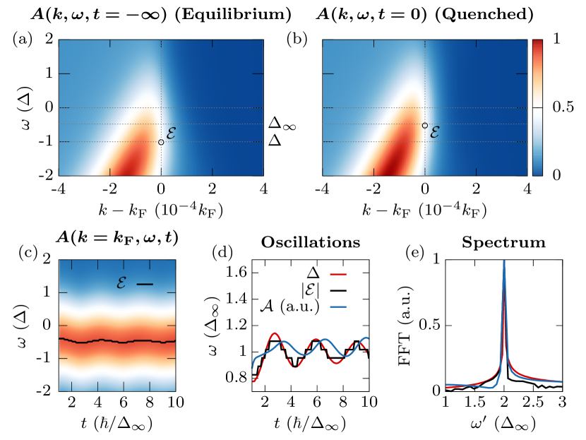
Figure 1: ARPES intensity of an $s$-wave superconductor after performing an interaction quench. (a) Equilibrium ARPES intensity $A(k,w,t=-\infty)$, the maximum of the energy distribution curve (EDC) at $k=k_{\mathrm{F}}$ is marked by a circle and labeled $\mathcal{E}$. The maximum is at $|\mathcal{E}|=\Delta$. (b) ARPES intensity $A(k,w,t=0)$ after the interaction quench, spectral weight is shifted towards the Fermi level. The maximum is at the reduced value $\Delta_{\infty}<|\mathcal{E}|<\Delta$. (c) Time evolution of the EDC at $k=k_{\mathrm{F}}$. See also Fig. 2. (d) Gap oscillations $\Delta(t)$, oscillations of the EDC maximum $|\mathcal{E}(t)|$ and amplitude oscillation $\mathcal{A}(t,k=k_{\mathrm{F}})$ of the ARPES intensity. The edges in $\mathcal{E}(t)$ are an artifact due to the finite frequency resolution. (e) Fourier transform of oscillations, all quantities oscillate with the Higgs frequency $\omega=2\Delta_{\infty}$. The probe pulse width is $\tau_{p}=1$ $\hbar/\Delta_{\infty}$.

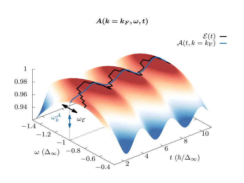
Figure 2: Time evolution of the EDC at $k=k_{\mathrm{F}}$. It corresponds to Fig. 1(c) plotted as a 3d plot for better visualization. There are two different kinds of dynamics: Oscillations in energy of the maximum of the EDC curve (black line) as defined in Eq. (18) with the momentum-independent frequency $\omega_{\mathcal{E}}=2\Delta_{\infty}$ and oscillations in the amplitude of the ARPES intensity (blue line) as defined in Eq. (19) with the momentum-dependent frequency $\omega_{\bm{k}}^{\mathcal{A}}=2\sqrt{\epsilon_{\bm{k}}^{2}+(\Delta_{\infty}f_{\bm{k}})^{2}}$. At $k=k_{\mathrm{F}}$ and $f_{\bm{k}}=1$, $\omega_{\bm{k}}^{\mathcal{A}}=\omega_{\mathcal{E}}=2\Delta_{\infty}$.

III.2 State quench for $d$-wave superconductor

After having considered the $s$-wave case with an isotropic interaction quench, we will proceed to a $d$-wave superconductor, which we will quench in different symmetry channels with the help of a state quench as defined in Sec. II.3. The symmetry function of a $d$-wave superconductor close to the Fermi level can be written as $f_{\bm{k}}=\cos(2\varphi)$, where $\varphi$ is the polar angle. In order to excite the system in a systematic way, we choose quench symmetries which are fundamental with respect to the lattice point group. To this end, the superconductor is quenched in all different symmetry channels for the $D_{4h}$ point group, which is the underlying lattice point group for the important $d$-wave example of cuprate superconductors. We define the following four quenches:

$$A_{1g}: \quad f_{\bm{k}}^{\mathrm{q}}=1\,,$$ (20a)

$$A_{2g}: \quad f_{\bm{k}}^{\mathrm{q}}=\sin(4\varphi)\,,$$ (20b)

$$B_{1g}: \quad f_{\bm{k}}^{\mathrm{q}}=\cos(2\varphi)\,,$$ (20c)

$$B_{2g}: \quad f_{\bm{k}}^{\mathrm{q}}=\sin(2\varphi)\,.$$ (20d)

The symmetry function and the quenched symmetry function, as well as the ARPES intensity after the quench, can be found in Fig. 3. First of all, in the equilibrium case, the ARPES intensity closely resembles the absolute value of the symmetry function. In the antinodal directions at $\varphi=[0,\pi/2,\pi,3\pi/2]$, a full open gap can be observed with $|\mathcal{E}|=\Delta$. Moving $\varphi$ towards the nodal directions $\varphi=[\pi/4,3\pi/4,5\pi/4,7\pi/4]$, the maximum $\mathcal{E}$ approaches zero.

The influence of the different quenches is also reflected in the change in the ARPES intensity. The $A_{1g}$- and $B_{2g}$-quenches shift the position of the nodes. In the case of the $A_{1g}$-quench, the shift is in opposite directions relative to the lobe maxima, which creates lobes with different sizes. The $B_{2g}$-quench shifts all nodes in the same direction, which results in a rotation of all lobes. This can be seen by a transfer of spectral weight above the Fermi level at exactly these points in the ARPES intensity. The $B_{1g}$-quench does not change the symmetry at all and the $A_{2g}$-quench only shifts weight inside the lobes, such that for these two quenches, no obvious change in the symmetry of the ARPES intensity is observable.

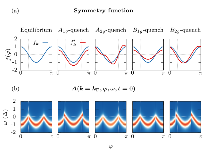
Figure 3: ARPES intensity of a $d$-wave superconductor after a state quench. (a) Symmetry function $f_{\bm{k}}$ (blue) and quenched symmetry function $f_{\bm{k}}^{\prime}$ (red) for different channels. (b) Corresponding ARPES intensity. A shift of nodal lines is reflected by a shift of spectral weight in the nodal region. The probe pulse width is $\tau_{p}=10$ $\hbar/\Delta_{\infty}$.

This fact is crucial for the induced Higgs oscillations of the gap, as for the $A_{1g}$- and $B_{2g}$-quenches, the shift of the nodal lines creates a second low-lying Higgs mode dynamically, whereas for the other two quenches, it will not. This can be seen in Fig. 4(a) and (c), where the oscillations of the order parameter and their Fourier transform is shown for the different quench symmetries. While the $B_{1g}$- and $A_{2g}$-quenches only show a single broad peak around $\omega=2\Delta_{\infty}$, the $A_{1g}$- and $B_{2g}$-quenches show a two peak or kink structure in the spectrum with one peak around $\omega=2\Delta_{\infty}$ and a second peak at lower frequencies. The same behavior is visible for nodal $s$-wave, which is discussed in appendix C and shown in Fig. 4(b) and (d). The usual $2\Delta$ Higgs mode corresponds to an oscillation in the ground state symmetry channel, whereas the low-lying Higgs mode corresponds to an oscillation in another symmetry channel [28]. The energies of these two modes are controlled by different quantities. While the energy of the $2\Delta$ Higgs mode is given by the value of the gap, i.e. $\Delta_{\infty}$ after the quench, the energy of the other mode is controlled by the strength of deviation from the ground state symmetry. Thus, for increasing quench strength, the energy of the $2\Delta$ Higgs mode decreases, while the energy of the low-lying Higgs mode increases. This is discussed in appendix D in more detail.

Now, we will analyze the amplitude oscillations of the ARPES intensity $\mathcal{A}(t)$ in more detail to gain a deeper understanding of the dynamic creation of the low-lying Higgs mode. According to the gap equation (3), the value of $\Delta(t)$ is obtained by a summation over the condensate $\braket{c_{-{\bm{k}}\downarrow}c_{{\bm{k}}\uparrow}}$(t). Both, the anomalous Green’s function $\braket{c_{-{\bm{k}}\downarrow}c_{{\bm{k}}\uparrow}}$(t) and the normal Green’s function $\braket{c_{{\bm{k}}\uparrow}^{\dagger}c_{{\bm{k}}\uparrow}}$(t) share a similar dynamic as their equations of motion are coupled. This can be seen in Eq. (35) in appendix D. Therefore, a momentum-resolved analysis of the ARPES intensity, i.e. $\mathcal{A}(t,k,\varphi)$, which is proportional to the normal Green’s function, can reveal important information about the dynamic processes. In comparison, an angle-resolved evaluation of the maximum of the EDC curve, i.e. $\mathcal{E}(t,\varphi)$, as considered in [37], does not give further insight as it traces only the momentum-averaged quantity $\Delta(t)$.

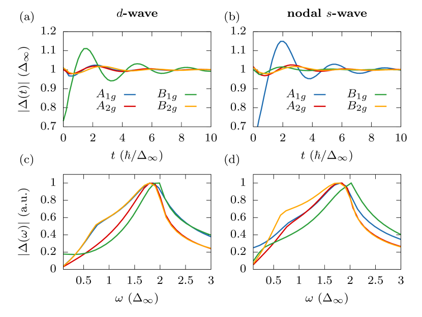
Figure 4: Gap dynamic of $d$-wave (left) and nodal $s$-wave (right). Top: Oscillations after quenching in the four fundamental symmetries defined in Eq. (20). The $B_{1g}$-quench for $d$-wave and the $A_{1g}$-quench for nodal $s$-wave induce stronger oscillations as these quenches are within the same symmetry channel as the gap symmetry. Bottom: Fourier transform of the gap oscillations. All energies are normalized to their individual $\Delta_{\infty}$.

To this end, we extract $\mathcal{A}(t,k,\varphi)$ and its frequency $\omega_{{\bm{k}}}^{\mathcal{A}}$ not only at $k=k_{\mathrm{F}}$ but for all points in momentum space and plot its distribution in Fig. 5(a) for a $d$-wave superconductor quenched in the $A_{1g}$- and $B_{1g}$-channels. The resulting frequencies are momentum-dependent yet do not depend on the quench. Namely, the frequency at each momentum point ${\bm{k}}$ is given by two times the quasiparticle energy

$$\omega_{{\bm{k}}}^{\mathcal{A}}=2\sqrt{\epsilon_{\bm{k}}^{2}+(\Delta_{\infty}f_{\bm{k}})^{2}}\,.$$ (21)

This result is derived in appendix D. The same result for $s$-wave symmetry and an interaction quench was also found in [23]. A comparison of the extracted frequencies and the analytic formula shows perfect agreement.

In the summation process of the gap equation, the frequency with the largest weight will dominate the oscillations. In the case of $s$-wave with $f_{\bm{k}}=1$, this turns out to be at $k=k_{F}$, where $\epsilon_{\bm{k}}=0$, which results in a single main frequency $\omega=2\Delta_{\infty}$. However, as the other frequencies still contribute, the superposition of all different frequencies drives the oscillations out of phase in the long-time limit, which results in the well-known $1/\sqrt{t}$ decay [21]. In the case of $d$-wave, there is a much larger variety of frequencies due to the angular dependence of the gap $\Delta_{\bm{k}}$. Therefore, the summation process creates a much stronger decay [24]. As the oscillations in $\mathcal{E}(t)$ correspond directly to the gap oscillations $\Delta(t)$, the damping due to the dephasing is also visible in this quantity. In contrast, the oscillations visible in $\mathcal{A}(t,k,\varphi)$ are undamped as they correspond to oscillations of the quasiparticles, which can be understood as a precession of pseudospins as shown in appendix D. In the gap equation, it is exactly this undamped oscillation of different momentum-dependent frequencies which is summed up leading to the dephasing effect and the damping of the collective Higgs oscillations. The analytic expression for the pseudospin precession derived in Eq. (36) in the appendix shows this undamped oscillation.

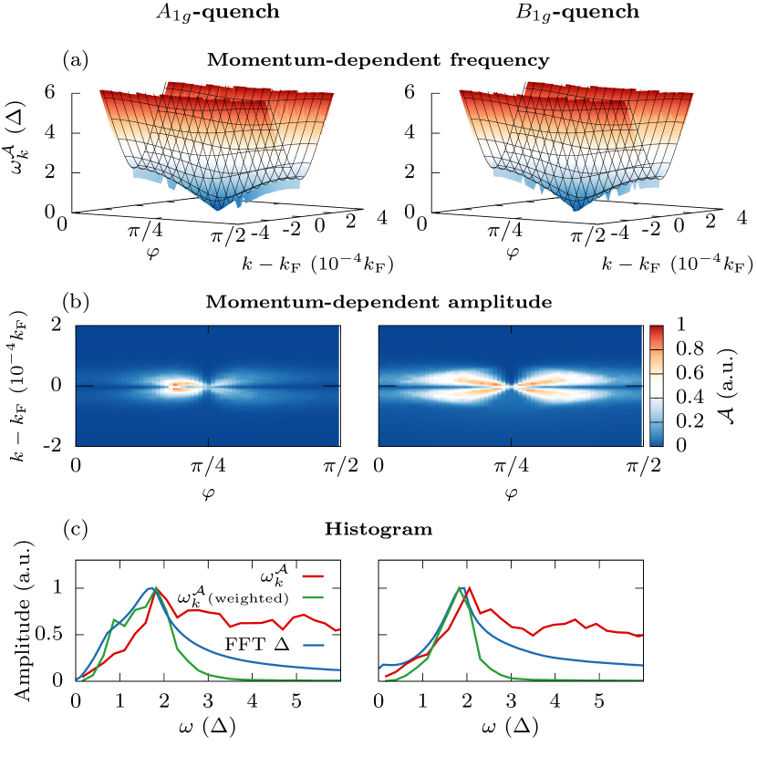
Figure 5: Frequency distribution of ARPES intensity oscillation for $A_{1g}$-quench (left) and $B_{1g}$-quench (right). (a) Momentum-dependent frequency $\omega_{\bm{k}}^{\mathcal{A}}$ of $\mathcal{A}(t,k,\varphi)$ (colored) compared with the theoretical formula from Eq. (21) (lines). (b) Momentum-dependent amplitudes of the oscillations. (c) Histogram of occurring frequencies compared with Fourier transform of gap oscillations. The probe pulse width is $\tau_{p}=1$ $\hbar/\Delta_{\infty}$.

The second low-lying frequency for certain quenches can be explained in the same picture. In Fig. 5(b), we show the extracted amplitudes for $\omega_{{\bm{k}}}^{\mathcal{A}}$ at each momentum point, which correspond to the actual weight for each frequency. While there is no difference in the frequency distribution between different quenches in Fig. 5(a), we can clearly see a difference in the amplitudes between the $A_{1g}$-quench, which shows a second peak in the Higgs oscillations, and the $B_{1g}$-quench, which shows no second peak. The change in symmetry due to the quench creates a strong asymmetry in the weights regarding the positive and negative lobe direction in the case of the $A_{1g}$-quench, while the amplitudes for the $B_{1g}$-quench are symmetric. This can result in the summation process in an additional enhancement of frequencies other than $\omega=2\Delta_{\infty}$. In Fig. 5(c), we show the histogram of the frequencies from all momentum points. The raw histogram (red curve) looks exactly the same for both quenches, with a peak at $\omega=2\Delta_{\infty}$ already without additional weighting. Now, if we weight the histogram with the amplitude of the oscillation, the picture changes (green curve). In the case of the $A_{1g}$-quench, a two peak or two kink structure becomes visible, very similar to the Fourier transform of the gap oscillation (blue curve), whereas the symmetric weighting in the case of the $B_{1g}$-quench only shows a one peak structure. Hence, a careful analysis of the momentum-resolved frequencies in the ARPES spectrum reveals the dynamic of the condensate and explains the underlying processes leading to the collective Higgs oscillations.

III.3 Analysis of oscillation phase

In the previous section we have seen how the oscillation of the ARPES intensity can provide a deep insight into the creation process of the collective Higgs oscillation of the order parameter. Now, we will analyze the phase of these oscillations at different points in momentum space to resolve the deformation dynamic of the condensate symmetry. We have seen that an $A_{1g}$-quench for $d$-wave changes the sizes of the positive and negative lobes, i.e. the lobes of one sign increase in size while the other decrease. The resulting deformation of the condensate symmetry will therefore be an oscillation, where the smaller lobe increases while the larger lobe decreases. Thus, the movement of the lobes is out of phase (see Fig. 6(a)).

The same quench applied to a nodal $s$-wave superconductor with $f_{\bm{k}}=\cos^{2}(2\varphi)$, which has the same nodal structure, will change its lobes all equally due to the same sign of the gap. The resulting oscillations are therefore in phase (see Fig. 6(b)). For comparison, the quenched symmetry function and the resulting ARPES intensities analogous to the $d$-wave case in Fig. 3 can be found in the appendix in Fig. 8. Even though the oscillation of the lobes is in phase for this quench, the gap oscillation shows a two peak structure (Fig. 4(d)) due to a shift of nodal lines. Thus, a comparison of the Higgs oscillation spectrum does not allow to distinguish between $d$-wave and nodal $s$-wave in this case.

To see whether we can observe the different condensate symmetry deformation for these two gap symmetries in the ARPES intensity, we extract the amplitude oscillations $\mathcal{A}(t,k=k_{\mathrm{F}},\varphi)$ at $\varphi=0$ and $\varphi=\pi/2$, i.e. at points in momentum space rotated by $\varphi=\pi/2$, which should oscillate with opposite phase in the case of $d$-wave and with the same phase for the nodal $s$-wave. The result can be found in Fig. 6(c) and (d) and confirms the expected oscillatory behavior. Oscillations of the amplitude provide therefore not only information about the amplitude of the gap but relative phase information from different points in momentum space can be extracted as well. This shows that the information obtainable from the time-dependent amplitude of the ARPES intensity allows to clearly trace the induced symmetry deformation and dynamic of the condensate in momentum space, e.g. to determine the movement of the $d$-wave or nodal $s$-wave lobes.

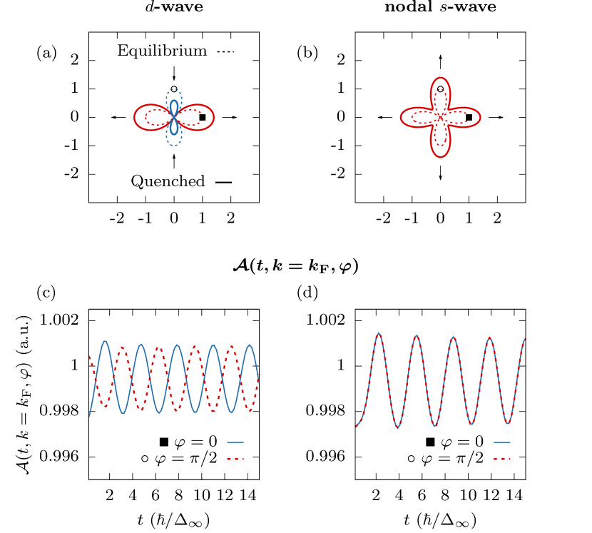
Figure 6: Oscillation of ARPES intensity after $A_{1g}$-quench for $d$-wave (left) and nodal $s$-wave (right) superconductor. (a),(b) Schematic picture of condensate symmetry in equilibrium (dotted) and quenched (solid lines). The arrows indicate the movement of the lobes. Points in momentum space rotated by $\pi/2$ oscillate with opposite phase in the case of $d$-wave and in phase in the case of nodal $s$-wave. For a $B_{1g}$-quench, the situation would be reversed. (c),(d) Time-dependent ARPES intensity. The oscillation of the ARPES intensity follows the oscillation of the lobes. The out of phase oscillation of $d$-wave lobes is clearly visible, in comparison to the in phase oscillations of the nodal $s$-wave. The probe pulse width is $\tau_{p}=0.2$ $\hbar/\Delta_{\infty}$.

IV Summary and Discussion

In this article we demonstrate how the collective Higgs oscillations of the superconducting order parameter can be traced back and be observed as oscillations of the ARPES intensity measured in THz tr-ARPES experiments. There are two kinds of dynamics, namely momentum-independent oscillations of the EDC maximum $\mathcal{E}(t)$, which directly correspond to oscillations of the energy gap $\Delta(t)$, and momentum-dependent oscillations of the amplitude of the ARPES intensity $\mathcal{A}(t,k,\varphi)$. While the EDC dynamic only reveals information about the momentum-averaged quantity $\Delta(t)$, the amplitude oscillation of the ARPES intensity allows to perform a momentum-resolved analysis of the condensate dynamic. Experimental conditions might dictate which quantity can be observed more easily. For this, further studies are required including realistic matrix element effects for the ARPES intensity as well as additional scattering channels influencing the amplitudes of the oscillations. What can be stated is that both quantities require short enough probe pulses to resolve the Higgs oscillations. The EDC maximum oscillations are restricted in their amplitude by the oscillation amplitude of the gap, which can be in the sub-percentage range depending on quench strength and gap symmetry. Increasing the quench strength also increases the amplitude oscillations up to a certain point beyond which the gap is quenched into a gapless regime. Additional heating effects, which are not considered here, restrict the maximum fluence of a quench pulse further, such that only small quenches can be implemented experimentally. In contrast, our calculation shows that the amplitude oscillations of the ARPES intensity can be up to several percentages in size also for small quench strength and thus, be much larger for certain conditions. However, they might be more difficult to resolve in general as oscillations in energy. Another difference can be found in the intrinsic damping. While the oscillations in $\mathcal{E}(t)$ are intrinsically damped due to dephasing, the oscillations in $\mathcal{A}(t,k,\varphi)$ are undamped. Yet, as the intrinsic damping follows only a power law, additional exponential damping will diminish this advantage when further scattering effects occur in an experiment.

A tracking of the amplitude oscillation frequencies $\omega_{\bm{k}}^{\mathcal{A}}$ of the ARPES intensity $\mathcal{A}(t,k,\varphi)$ at different momenta leads to a deeper understanding of the microscopic creation process of collective Higgs oscillations $\Delta(t)$. While the frequencies can be described with a single formula independent of gap- and quench symmetry, the relative weight of each frequency contributing in the collective amplitude oscillation of the order parameter is determined by the gap- and quench-symmetry in a nontrivial way. If there are asymmetries in the weights, additional Higgs modes can appear, which are dynamically created due to quenching the condensate in a symmetry channel different from its equilibrium value.

Furthermore, quenching the condensate in defined symmetry channels and observing the oscillation phase of the ARPES intensity allows to resolve the symmetry deformation and dynamic of the condensate. This condensate dynamic depends on the gap and quench symmetry. In this paper, the quench symmetry for a certain gap was given such that the resulting symmetry deformation dynamic of the condensate, like an in-phase or out-of-phase oscillation of lobes of a $d$-wave or nodal $s$-wave superconductor are clearly defined. Importantly, this explicit construction of a quench symmetry allows to distinguish between the two different gaps with same nodal structure but different phase.

Whether and how all considered quenches can be realized experimentally is an open question and beyond the scope of this paper; however, there are several promising possibilities. In-plane excitations can lead to symmetry breaking due to the small but non-vanishing photon momentum [28], which allows to quench the system asymmetrically with respect to its ground state symmetry. Such momentum transfer can be enhanced and controlled in more detail in transient grating setups [39, 40] or four-wave mixing experiments [41]. Once tailored quenches are realized experimentally, a new spectroscopic tool will be available to gain phase-sensitive information about the gap symmetry of unconventional superconductors.

Appendix A Equations of motion

Heisenberg’s equation of motion Eq. (9) for the time-dependent quasiparticle operators $\alpha_{\bm{k}}^{\dagger}(t)$ and $\beta_{\bm{k}}^{\dagger}(t)$ can be evaluated by using the ansatz in Eq. (10). From the resulting equations, a comparison of coefficients leads to a set of coupled finite hierarchy differential equations for the prefactors

$$\partial_{t}a_{0{\bm{k}}}(t)=\frac{\mathrm{i}}{\hbar}\Bigg{[}R_{\bm{k}}(t)\Big{[}a_{0{\bm{k}}}(t)\Big{(}|a_{0{\bm{k}}}(t)|^{2}+|a_{1{\bm{k}}}(t)|^{2}-|b_{1{\bm{k}}}(t)|^{2}\Big{)}-a_{1{\bm{k}}}(t)b_{0{\bm{k}}}(t)b_{1{\bm{k}}}^{*}(t)\Big{]}$$

$$\qquad\qquad\qquad+C_{\bm{k}}(t)\Big{[}a_{0{\bm{k}}}(t)\Big{(}a_{0{\bm{k}}}(t)b_{1{\bm{k}}}(t)+a_{1{\bm{k}}}(t)b_{0{\bm{k}}}(t)\Big{)}\Big{]}+C_{\bm{k}}^{*}(t)\Big{[}b_{1{\bm{k}}}^{*}(t)\Big{(}|a_{0{\bm{k}}}(t)|^{2}+|a_{1{\bm{k}}}(t)|^{2}\Big{)}\Big{]}\Bigg{]}\,,$$ (22a)

$$\partial_{t}a_{1{\bm{k}}}(t)=\frac{\mathrm{i}}{\hbar}\Bigg{[}-R_{\bm{k}}\Big{[}a_{1{\bm{k}}}(t)\Big{(}|b_{0{\bm{k}}}(t)|^{2}-|a_{1{\bm{k}}}(t)|^{2}-|a_{0{\bm{k}}}(t)|^{2}\Big{)}+a_{0{\bm{k}}}(t)b_{0{\bm{k}}}^{*}(t)b_{1{\bm{k}}}(t)\Big{]}$$

$$\qquad\qquad\qquad+C_{\bm{k}}(t)\Big{[}a_{0{\bm{k}}}(t)a_{1{\bm{k}}}(t)b_{1{\bm{k}}}(t)+a_{1{\bm{k}}}(t)^{2}b_{0{\bm{k}}}(t)\Big{]}+C_{\bm{k}}^{*}(t)\Big{[}b_{0{\bm{k}}}^{*}(t)\Big{(}|a_{0{\bm{k}}}(t)|^{2}+|a_{1{\bm{k}}}(t)|^{2}\Big{)}\Big{]}\Bigg{]}\,,$$ (22b)

$$\partial_{t}b_{0{\bm{k}}}(t)=\frac{\mathrm{i}}{\hbar}\bigg{[}R_{\bm{k}}(t)\Big{[}b_{0{\bm{k}}}(t)\Big{(}|b_{0{\bm{k}}}(t)|^{2}+|b_{1{\bm{k}}}(t)|^{2}-|a_{1{\bm{k}}}(t)|^{2}\Big{)}-a_{0{\bm{k}}}(t)a_{1{\bm{k}}}^{*}(t)b_{1{\bm{k}}}(t)\Big{]}$$

$$\qquad\qquad\qquad-C_{\bm{k}}\Big{[}a_{1{\bm{k}}}(t)b_{0{\bm{k}}}(t)^{2}+a_{0{\bm{k}}}(t)b_{0{\bm{k}}}(t)b_{1{\bm{k}}}(t)\Big{]}-C_{\bm{k}}^{*}\Big{[}a_{1{\bm{k}}}^{*}(t)\Big{(}|b_{0{\bm{k}}}(t)|^{2}+|b_{1{\bm{k}}}(t)|^{2}\Big{)}\Big{]}\bigg{]}\,,$$ (22c)

$$\partial_{t}b_{1{\bm{k}}}(t)=\frac{\mathrm{i}}{\hbar}\bigg{[}-R_{\bm{k}}(t)\Big{[}b_{1{\bm{k}}}(t)\Big{(}|a_{0{\bm{k}}}(t)|^{2}-|b_{0{\bm{k}}}(t)|^{2}-|b_{1{\bm{k}}}(t)|^{2}\Big{)}+a_{0{\bm{k}}}^{*}(t)a_{1{\bm{k}}}(t)b_{0{\bm{k}}}(t)\Big{]}$$

$$\qquad\qquad\qquad-C_{\bm{k}}\Big{[}a_{1{\bm{k}}}(t)b_{0{\bm{k}}}(t)b_{1{\bm{k}}}(t)+a_{0{\bm{k}}}(t)b_{1{\bm{k}}}(t)^{2}\Big{]}-C_{\bm{k}}^{*}(t)\Big{[}a_{0{\bm{k}}}^{*}(t)\Big{(}|b_{0{\bm{k}}}(t)|^{2}+|b_{1{\bm{k}}}(t)|^{2}\Big{)}\Big{]}\bigg{]}\,.$$ (22d)

The initial values for the prefactors can be derived from the initial values of the quasiparticle expectation values. The time-dependent quasiparticle expectation values expressed within the iterated equation of motion ansatz assuming that the system is in equilibrium for $T=0$ read

$$\braket{\alpha_{\bm{k}}^{\dagger}(t)\alpha_{{\bm{k}}}(t^{\prime})} =a_{1{\bm{k}}}(t)a_{1{\bm{k}}}^{*}(t^{\prime})\,,$$ (23a)

$$\braket{\beta_{\bm{k}}^{\dagger}(t)\beta_{{\bm{k}}}(t^{\prime})} =b_{1{\bm{k}}}(t)b_{1{\bm{k}}}^{*}(t^{\prime})\,,$$ (23b)

$$\braket{\alpha_{\bm{k}}(t)\beta_{{\bm{k}}}(t^{\prime})} =a_{0{\bm{k}}}^{*}(t)b_{1{\bm{k}}}^{*}(t^{\prime})\,,$$ (23c)

$$\braket{\alpha_{\bm{k}}^{\dagger}(t)\beta_{{\bm{k}}}^{\dagger}(t^{\prime})} =a_{1{\bm{k}}}(t)b_{0{\bm{k}}}(t^{\prime})\,.$$ (23d)

Parameter	Value
Dispersion $\epsilon_{\bm{k}}$	$t{\bm{k}}^{2}-\epsilon_{\mathrm{F}}$
Dispersion parameter $t$	$2005.25\,\mathrm{meV}$
Fermi energy $\epsilon_{\mathrm{F}}$	$9470\,\mathrm{meV}$
Gap value $\Delta$	$1.35\,\mathrm{meV}$
Energy cutoff $\epsilon_{\mathrm{c}}$	$8.3\,\mathrm{meV}$
Interaction quench strength $g_{\mathrm{i}}$	$0.8$
State quench strength $g_{\mathrm{s}}$	$0.4$
Temperature $T$	$0\,\mathrm{K}$
Radial discretization points $N_{k}$	$1000$
Azimuthal discretization points $N_{\varphi}$	$1000$

Table 1: Parameters used in the numerical calculation. The values correspond to material parameters of lead, following [31]. All results depend only quantitatively on the parameters and can be rescaled to any other material values.

To derive this result, we used the fact that for $T=0$, all equilibrium quasiparticle expectation values, i.e. $\braket{\alpha_{\bm{k}}^{\dagger}\alpha_{{\bm{k}}}}=0$ etc. are zero. For $t=t^{\prime}=0$, we easily find

$$a_{0{\bm{k}}}(0) =b_{0{\bm{k}}}(0)=1\,,$$ (24a)

$$a_{1{\bm{k}}}(0) =b_{1{\bm{k}}}(0)=0\,,$$ (24b)

i.e. $\alpha_{{\bm{k}}}^{\dagger}(0)=\alpha_{\bm{k}}^{\dagger}$ and $\beta_{{\bm{k}}}^{\dagger}(0)=\beta_{\bm{k}}^{\dagger}$. The solution for a nonequilibrium distribution is straight forward as well, by using the respective initial values for quasiparticle expectation values. However, we found it advantageous for more numerical stability to first use the relation

$$|a_{0{\bm{k}}}(t)|^{2}+|a_{1{\bm{k}}}(t)|^{2} =1\,,$$ (25a)

$$|b_{0{\bm{k}}}(t)|^{2}+|b_{1{\bm{k}}}(t)|^{2} =1\,,$$ (25b)

following from the anticommutation rules for the time-dependent Heisenberg operators, to rewrite Eq. (23) as

$$\braket{\alpha_{\bm{k}}^{\dagger}\alpha_{{\bm{k}}}}(0) =1-|a_{0{\bm{k}}}(0)|^{2}\,,$$ (26a)

$$\braket{\beta_{\bm{k}}^{\dagger}\beta_{{\bm{k}}}}(0) =1-|b_{0{\bm{k}}}(0)|^{2}\,,$$ (26b)

$$\braket{\alpha_{\bm{k}}\beta_{{\bm{k}}}}(0) =a_{0{\bm{k}}}^{*}(0)b_{1{\bm{k}}}^{*}(0)\,,$$ (26c)

$$\braket{\alpha_{\bm{k}}^{\dagger}\beta_{{\bm{k}}}^{\dagger}}(0) =a_{1{\bm{k}}}(0)b_{0{\bm{k}}}(0)\,,$$ (26d)

such that the solution reads

$$a_{0{\bm{k}}}(0) =\sqrt{1-\braket{\alpha_{{\bm{k}}}^{\dagger}\alpha_{{\bm{k}}}}(0)}\,,$$ (27a)

$$b_{0{\bm{k}}}(0) =\sqrt{1-\braket{\beta_{{\bm{k}}}^{\dagger}\beta_{{\bm{k}}}}(0)}\,,$$ (27b)

$$a_{1{\bm{k}}}(0) =\frac{\braket{\alpha_{{\bm{k}}}^{\dagger}\beta_{{\bm{k}}}^{\dagger}}(0)}{\sqrt{1-\braket{\beta_{{\bm{k}}}^{\dagger}\beta_{{\bm{k}}}}(0)}}\,,$$ (27c)

$$b_{1{\bm{k}}}(0) =\frac{\braket{\alpha_{{\bm{k}}}\beta_{{\bm{k}}}}^{*}(0)}{\sqrt{1-\braket{\alpha_{{\bm{k}}}^{\dagger}\alpha_{{\bm{k}}}}(0)}}\,.$$ (27d)

This prevents dividing by zero in the calculation of $a_{1{\bm{k}}}(0)$ and $b_{1{\bm{k}}}(0)$.

The initial values $\braket{\alpha_{{\bm{k}}}^{\dagger}\alpha_{{\bm{k}}}}(0)$ etc. in the state quenched case are derived as follow. For $T=0$, the equilibrium electron expectation values read

$$\braket{c_{-{\bm{k}}\downarrow}c_{{\bm{k}}\uparrow}} =\frac{\Delta_{\bm{k}}}{2E_{\bm{k}}}\,,$$ (28a)

$$\braket{c_{{\bm{k}}\uparrow}^{\dagger}c_{-{\bm{k}}\downarrow}^{\dagger}} =\frac{\Delta_{\bm{k}}^{*}}{2E_{\bm{k}}}\,,$$ (28b)

$$\braket{c_{{\bm{k}}\uparrow}^{\dagger}c_{{\bm{k}}\uparrow}} =\frac{1}{2}-\frac{\epsilon_{\bm{k}}}{2E_{\bm{k}}}\,,$$ (28c)

$$\braket{c_{-{\bm{k}}\downarrow}c_{-{\bm{k}}\downarrow}^{\dagger}} =\frac{1}{2}+\frac{\epsilon_{\bm{k}}}{2E_{\bm{k}}}\,.$$ (28d)

Using the definition of the Bogoliubov transformation in Eq. (4) one can derive the corresponding expressions for the quasiparticle expectation values. In the state quench, all occurring symmetry functions $f_{\bm{k}}$ are replaced by the modified symmetry function $f_{\bm{k}}^{\prime}$. These expectation values are then used as initial values for the calculation.

Appendix B Influence of probe pulse width

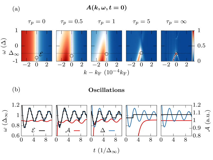
Figure 7: Influence of probe pulse width on ARPES spectrum and its time evolution for an s-wave superconductor after an interaction quench. For decreasing probe pulse width (right to left), the energy resolution decreases while the time-resolution increases. The edges in $\mathcal{E}$ are an artifact due to the finite frequency resolution. The decreased amplitude of the ARPES intensity in the beginning for larger pulse widths $\tau_{\mathrm{p}}$ results from decreased weight due to the cutoff of the probe pulse envelope at $t=0$.

The probe pulse width determines both the energy resolution in the spectrum and the time resolution in the dynamic [44]. If the probe pulse is very long compared to the intrinsic oscillations of the system, i.e. $\tau_{p}\gg\hbar/(2\Delta_{\infty})$, it can only detect the average value of the oscillations, which results in constant quantities $\mathcal{E}$ and $\mathcal{A}$. However, if the probe pulse is short in time, i.e. shorter than the intrinsic oscillation period of the system, it can scan the oscillations which leads to oscillations in the ARPES intensity in energy and amplitude.

In Fig. 7, the ARPES intensity of an $s$-wave superconductor after an interaction quench is shown for different probe pulse widths. An infinite long probe pulse with $\tau_{p}=\infty$ leads to a very sharp ARPES intensity in energy. However, no oscillations in the ARPES intensity can be observed in this case (black and red curve), despite the oscillations in the gap (blue curve). For decreasing probe pulse width, the energy resolution of the ARPES intensity decreases and the ARPES intensity peak becomes broader. Simultaneously, the time-resolution increases and oscillations of the EDC maximum $\mathcal{E}(t)$ and the ARPES intensity amplitude $\mathcal{A}(t)$ can be observed.

Appendix C State quench for nodal $s$-wave superconductor

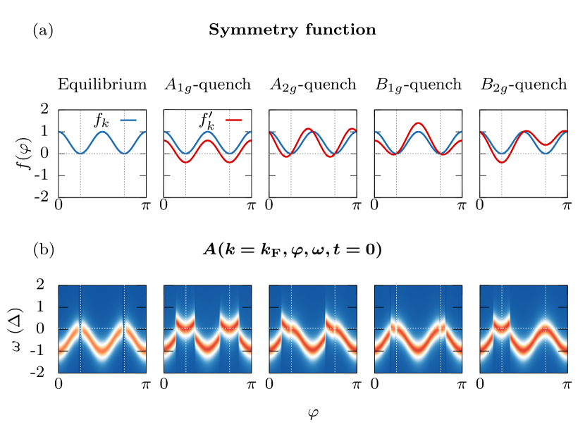
Figure 8: ARPES intensity of a nodal $s$-wave superconductor after a state quench. Top: Symmetry function $f_{\bm{k}}$ (blue) and quenched symmetry function $f_{\bm{k}}^{\prime}$(red) for different channels. Bottom: Corresponding ARPES intensity, shift of nodal lines is reflected by a shift of spectral weight in the nodal region. The probe pulse width is $\tau_{p}=10$ $\hbar/\Delta_{\infty}$.

In analogy to Sec. III.2 and Fig. 3, we quench a nodal $s$-wave superconductor in all symmetry channels of the $D_{4h}$ lattice point group. The result can be found in Fig. 8. In the areas, where the quench shifts nodal lines, we can observe a corresponding shift in spectral weight. If one calculates the resulting gap oscillations shown in Fig. 4, one can observe a two peak or kink structure for all quenches. We can understand this by the fact that all quenches shift the nodal lines such that there is an asymmetry in the weights of the $k$-dependent frequencies. In the case of the $B_{1g}$-quench, this shift is smaller compared to the other quenches, which results in a lower frequency of the second Higgs mode. In general, the energy of the dynamically created Higgs mode depends on the quench strength, i.e. the deviation from the equilibrium state.

Appendix D Momentum-dependent frequency

If we are only interested in the dynamic of the gap and expectation values at equal times, we can formulate the BCS Hamiltonian in Anderson’s pseudopin representation [45] and solve the resulting Bloch equations similar to [28]. The pseudospin is defined as

$$\bm{\sigma}_{\bm{k}} =\frac{1}{2}\Psi_{\bm{k}}^{\dagger}\bm{\tau}\Psi_{\bm{k}}$$ (29)

with the Nambu-Gorkov spinor $\Psi_{\bm{k}}^{\dagger}=\begin{pmatrix}c_{{\bm{k}}\uparrow}&c^{\dagger}_{-{\bm{k}}\downarrow}\end{pmatrix}$ and the Pauli matrices $\tau^{i}$. The $x$-component corresponds to the real part of the anomalous Green’s function $\braket{c_{-{\bm{k}}\downarrow}c_{{\bm{k}}\uparrow}}+\braket{c_{{\bm{k}}\uparrow}^{\dagger}c_{-{\bm{k}}\downarrow}^{\dagger}}$, while the $z$-component corresponds to the normal Green’s function $\braket{c_{{\bm{k}}\uparrow}^{\dagger}c_{{\bm{k}}\uparrow}}-\braket{c_{-{\bm{k}}\downarrow}c_{-{\bm{k}}\downarrow}^{\dagger}}$. The BCS Hamiltonian can be written as

$$H(t) =\sum_{\bm{k}}\bm{b}_{\bm{k}}(t)\bm{\sigma}_{\bm{k}}$$ (30)

with the pseudomagnetic field $\bm{b}_{\bm{k}}(t)=\left(-2\Delta(t)f_{\bm{k}},0,2\epsilon_{\bm{k}}\right)$ and the gap equation reads

$$\Delta(t) =V\sum_{\bm{k}}f_{\bm{k}}\braket{\sigma_{\bm{k}}^{x}}(t)\,.$$ (31)

Hereby, we assume a real gap, such that the $y$-component, which corresponds to the imaginary part of the gap, is zero. Heisenberg’s equations of motion for the pseudospin take the form of Bloch equations

$$\partial_{t}\braket{\bm{\sigma}_{\bm{k}}}(t) =\bm{b}_{\bm{k}}(t)\times\braket{\bm{\sigma}_{\bm{k}}}(t)\,.$$ (32)

We can linearize these equations for small deviations from the initial values

$$\braket{\bm{\sigma}_{\bm{k}}}(t) =\braket{\bm{\sigma}_{\bm{k}}}(0)+\braket{\delta\bm{\sigma}_{\bm{k}}}(t)\,,$$ (33a)

$$\Delta(t) =\Delta(0)+\delta\Delta(t)\,,$$ (33b)

where $\braket{\bm{\sigma}_{\bm{k}}}(0)$ is the quenched pseudospin expectation value at $t=0$ with

$$\braket{\sigma_{\bm{k}}^{x}}(0) =\braket{\sigma_{\bm{k}}^{x}}^{\prime}=\frac{\Delta_{\bm{k}}^{\prime}}{2E_{\bm{k}}^{\prime}}\,,$$ (34a)

$$\braket{\sigma_{\bm{k}}^{z}}(0) =\braket{\sigma_{\bm{k}}^{z}}^{\prime}=-\frac{\epsilon_{\bm{k}}}{2E_{\bm{k}}^{\prime}}$$ (34b)

according to Sec. II.3 in the main text. Using this ansatz while neglecting all products in higher order of the deviations, we can write the Bloch equations in Laplace space for complex frequency $s$ as

$$s\braket{\delta\sigma_{\bm{k}}^{x}}(s) =-2\epsilon_{\bm{k}}\braket{\delta\sigma_{\bm{k}}^{y}}(s)\,,$$ (35a)

$$s\braket{\delta\sigma_{\bm{k}}^{y}}(s) =\frac{2\epsilon_{\bm{k}}}{s}\frac{\Delta f^{\prime}_{\bm{k}}-\Delta(0)f_{\bm{k}}}{2E^{\prime}_{\bm{k}}}$$

$$\quad+2\epsilon_{\bm{k}}\braket{\delta\sigma_{\bm{k}}^{x}}(s)$$

$$\quad+2\Delta(0)f_{\bm{k}}\braket{\delta\sigma_{\bm{k}}^{z}}(s)$$

$$\quad-2\epsilon_{\bm{k}}\frac{f_{\bm{k}}}{2E^{\prime}_{\bm{k}}}\delta\Delta(s)\,,$$ (35b)

$$s\braket{\delta\sigma_{\bm{k}}^{z}}(s) =-2f_{\bm{k}}\Delta(0)\braket{\delta\sigma_{\bm{k}}^{y}}(s)\,.$$ (35c)

Solving for the $x$- and $z$-component, it follows

$$\braket{\delta\sigma_{\bm{k}}^{x}}(s) =\frac{2\epsilon^{2}E_{\bm{k}}^{\prime}(\frac{\Delta(0)f_{\bm{k}}-\Delta f_{\bm{k}}^{\prime}}{s}+f_{\bm{k}}\delta\Delta(s))}{4\epsilon^{2}+4\Delta(0)^{2}f_{\bm{k}}^{2}+s^{2}}\,,$$ (36a)

$$\braket{\delta\sigma_{\bm{k}}^{z}}(s) =\frac{2\epsilon\Delta(0)f_{\bm{k}}E_{\bm{k}}^{\prime}(\frac{\Delta(0)f_{\bm{k}}-\Delta f_{\bm{k}}^{\prime}}{s}+f_{\bm{k}}\delta\Delta(s))}{4\epsilon^{2}+4\Delta(0)^{2}f_{\bm{k}}^{2}+s^{2}}$$ (36b)

and the solution for the gap reads

$$\delta\Delta(s) =\frac{F_{2}(s)}{1-F_{1}(s)}$$ (37)

with

$$F_{1}(s) =C-V\sum_{\bm{k}}f_{\bm{k}}^{2}\frac{s^{2}+4\Delta(0)^{2}f_{\bm{k}}^{2}}{2E^{\prime}_{\bm{k}}\left(s^{2}+4\epsilon_{\bm{k}}^{2}+4\Delta(0)^{2}f_{\bm{k}}^{2}\right)}\,,$$ (38a)

$$F_{2}(s) =\frac{\Delta(0)}{s}\left(C-1\right)+\frac{1}{s}V\sum_{\bm{k}}f_{\bm{k}}(\Delta f^{\prime}_{\bm{k}}-\Delta(0)f_{\bm{k}})\frac{s^{2}+4\Delta(0)^{2}f_{\bm{k}}^{2}}{2E^{\prime}_{\bm{k}}(s^{2}+4\epsilon_{\bm{k}}^{2}+4\Delta(0)^{2}f_{\bm{k}}^{2})}\,.$$ (38b)

with $C=V\sum_{\bm{k}}\frac{f_{\bm{k}}^{2}}{2E^{\prime}_{\bm{k}}}$. An inverse Laplace transform yields

$$F_{1}(t) =C-V\sum_{\bm{k}}f_{\bm{k}}^{2}\Big{(}\frac{\delta(t)}{2E_{\bm{k}}^{\prime}}-\frac{2\epsilon_{\bm{k}}^{2}}{E_{\bm{k}}^{\prime}\omega_{\bm{k}}}\sin(\omega_{\bm{k}}t)\Big{)}\,,$$ (39a)

$$F_{2}(t) =\Delta(0)\left(C-1\right)+V\sum_{\bm{k}}f_{\bm{k}}(\Delta f^{\prime}_{\bm{k}}-\Delta(0)f_{\bm{k}})\Big{(}\frac{2\Delta(0)^{2}f_{\bm{k}}^{2}+\epsilon_{\bm{k}}^{2}\cos(\omega_{\bm{k}}t)}{E_{\bm{k}}^{\prime}\omega_{\bm{k}}^{2}}\Big{)}\,,$$ (39b)

where $\omega_{\bm{k}}=2\sqrt{\epsilon_{\bm{k}}^{2}+\Delta(0)^{2}f_{\bm{k}}^{2}}$. In the linear regime, we can approximate $\Delta(0)\approx\Delta_{\infty}$, such that we arrive at the formula Eq. (21) from the main text. We can see that the main oscillation frequency of the summand in the gap equation and both the anomalous and normal Green’s function, i.e. the $x$- and $z$-component of the pseudospin in Eq. (36) is given by $\omega_{\bm{k}}^{\mathcal{A}}$. The frequency is independent of the quench, however the individual weighting in momentum space, i.e. the amplitudes of each frequencies depend heavily on the quench. Namely, the prefactors, controlled by the gap symmetry $f_{\bm{k}}$ and quenched symmetry $f_{\bm{k}}^{\prime}$, determine the dominating frequency in the summation process in a nontrivial way.

We can see the energy scales of the collective Higgs modes in more detail, by evaluating the $k$-sum in $F_{1}(s)$ or $F_{2}(s)$. For this, the sum is replaced by an integral using polar coordinates, i.e. $V\sum_{\bm{k}}\rightarrow\lambda\int_{-\infty}^{\infty}\,\mathrm{d}\epsilon\,\int_{0}^{2\pi}\,\mathrm{d}\varphi$, where $\lambda=VD(\epsilon_{\mathrm{F}})$ with $D(\epsilon_{\mathrm{F}})$ the density of states at the Fermi level. Following [28], one finds

$$F_{1}(s)\propto\int_{0}^{2\pi}\frac{\sqrt{s^{2}+4\Delta(0)^{2}f(\varphi)^{2}}}{\sqrt{s^{2}+4(\Delta(0)^{2}f(\varphi)^{2}-\Delta^{2}f^{\prime}(\varphi)^{2})}}$$ (40)

and a similar expression for $F_{2}(s)$. Here, two energy scales appear. The term $\sqrt{s^{2}+4\Delta(0)^{2}f(\varphi)^{2}}$ determines the usual $2\Delta$ Higgs mode, whereas the term $\sqrt{s^{2}+4(\Delta(0)^{2}f(\varphi)^{2}-\Delta^{2}f^{\prime}(\varphi)^{2})}$ determines the energy of the second low-lying Higgs mode. For small quenches $g\approx 0$, the quenched symmetry function is $f^{\prime}(\varphi)\approx f(\varphi)$ and the second Higgs mode softens. For increasing quench strength, the difference $\Delta(0)^{2}f(\varphi)^{2}-\Delta^{2}f^{\prime}(\varphi)^{2}$ increases, resulting in an increase of the energy. In contrast, the $2\Delta$ Higgs mode decreases as the gap is reduced more. Yet, to obtain the exact energies, the integral has to be evaluated numerically as the whole expression is nontrivial.

The gap oscillations are damped with $1/t^{n}$, where $n=1/2$ for $s$-wave and $n>1/2$ for $d$-wave. This is a dephasing effect as oscillations of slightly different frequency are summed up in the gap equation. In contrast, the oscillations of the quasiparticles or pseudospins, which are the quantities which are summed up in the gap equation, are undamped. This can be seen in the expression for the pseudospins in Eq. (36). As an example the expression for the $z$-component reads

$$\braket{\sigma_{\bm{k}}^{z}}(s) =\frac{a}{s(b^{2}+s^{2})}+\frac{c}{b^{2}+s^{2}}\delta\Delta(s)\,,$$ (41)

where $a$, $b$, $c$ are $s$-independent constants. The inverse Laplace transform of the first term yields $a/b^{2}-a\cos(bt)/b^{2}$, which contains an undamped oscillatory part. As a result, the considered amplitude oscillations $\mathcal{A}(t,k,\varphi)$ in this work are undamped as well.

Appendix E Influence of system parameters

Higgs oscillations are a collective oscillation of the order parameter. Thus, a variation of system parameters only quantitatively changes the oscillations but do not affect the overall collective excitation. To demonstrate that the induced Higgs oscillation do not depend on system parameters, we show results for a single-band tight-binding dispersion on a square lattice, where we vary the filling and quench strength. The dispersion reads

$$\epsilon_{\bm{k}} =-2t(\cos k_{x}+\cos k_{y})-\epsilon_{\mathrm{F}}$$ (42)

where we chose $t=200$ meV, $\Delta=30$ meV, $\epsilon_{\mathrm{c}}=60$ meV, $N_{k}=2000$ and $N_{\varphi}=1000$, which is in the order of numerical values found e.g. in cuprates.

In Fig. 9(a) and (b), we show the results for a $d$-wave order parameter which we quench in the $A_{1g}$ channel with a fixed strength of $g=0.4$. We vary the filling by varying the Fermi energy from $\epsilon_{\mathrm{F}}=-100$ meV to $\epsilon_{\mathrm{F}}=100$ meV. This changes the Fermi surface from nearly circular to discontiguous Fermi pockets at the diagonals. First of all, independent of the parameters, Higgs oscillations are always excited as shown in Fig. 9(a) and in all cases, two Higgs modes are visible as it can be seen in Fig. 9(b). As the Fermi surface changes for different fillings, the same quench strength $g$ has a different strong quench effect on the system, yet, the result is qualitatively the same. As we have shown in this paper the ARPES intensity directly reflects the collective gap oscillations and the oscillations of the underlying condensate. Thus, the qualitative invariance of the gap oscillations under variation of system parameters is also found in the oscillations of the ARPES intensity.

Quantitatively, the following differences are visible. In the half-filling case $\epsilon_{\mathrm{F}}=0$, where the Fermi surface has the shape of a square with the corners in the antinodal direction, the $2\Delta_{\infty}$ peak is sharper compared to the other cases. This is perfectly understandable with our analysis of the main text regarding the emerging of the Higgs modes. Due to the position of the corners in the antinodal direction, there is more weight in this region and the corresponding frequencies contribute more. As the frequency in the antinodal direction at the Fermi level is given by the full open gap $2\Delta_{\infty}$, this frequency dominates the resulting spectrum.

Another difference is visible for discontiguous Fermi surfaces with $\epsilon_{\mathrm{F}}>0$. Here, there is no Fermi surface in the antinodal direction and thus, less weight for the $2\Delta_{\infty}$ oscillation. As a consequence, the main peak is slightly shifted to lower frequencies.

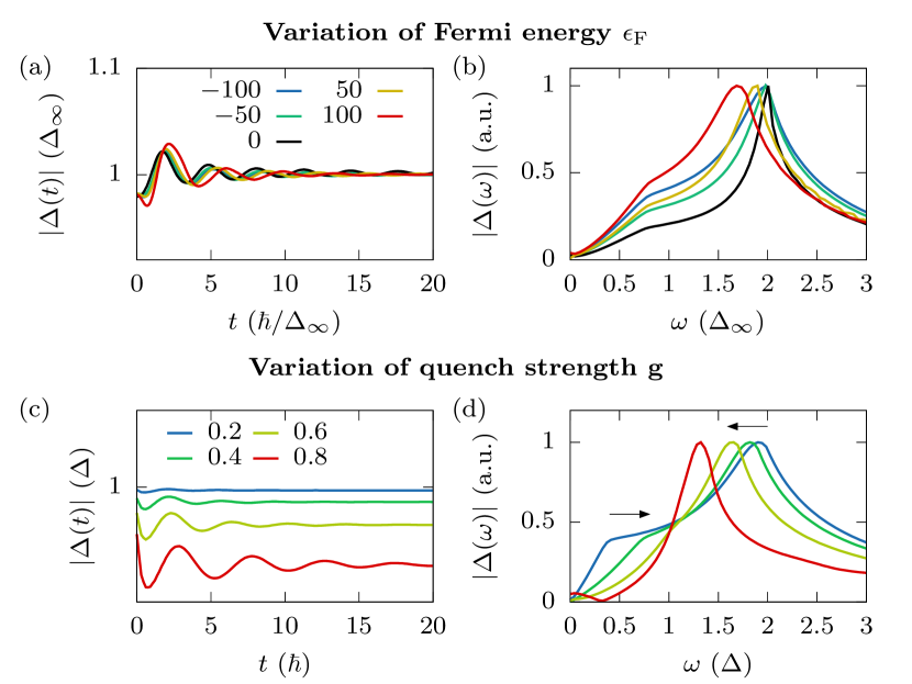
Figure 9: Higgs oscillations and spectrum for a $d$-wave order parameter quenched in the $A_{1g}$ channel for varying parameters using the tight-binding dispersion Eq. (42). (a) and (b) The Fermi energy $\epsilon_{\mathrm{F}}$ is varied from negative to positive values, which results in a change in the Fermi surface form nearly circular to discontiguous Fermi pockets. In all cases, 2 Higgs modes occur, yet, the relative weight of the occurring frequencies depends on the Fermi surface. (c) and (d) The quench strength $g$ is varied. For increasing quench strength, the $2\Delta_{\infty}$ Higgs mode is shifted to lower energies, while the low-lying Higgs mode is shifted to higher energies.

In Fig. 9(c) and (d), we fix the filling at $\epsilon_{\mathrm{F}}=-100$ meV and vary the quench strength using $g=[0.2,0.4,0.6,0.8]$. We observe that the gap is reduced more for stronger quenches, i.e. $\Delta_{\infty}$ decreases. As a consequence, the main oscillation frequency of the $2\Delta_{\infty}$ Higgs mode decreases as well, which can already be seen in the oscillations in Fig. 9(c) but more clearly in Fig. 9(d) by a shift of the main peak to lower frequencies. In contrast, as also discussed in appendix D, the energy of the low-lying Higgs mode increases.

References

- Damascelli et al. [2003] A. Damascelli, Z. Hussain, and Z.-X. Shen, Angle-resolved photoemission studies of the cuprate superconductors, Rev. Mod. Phys. 75, 473 (2003).
- Freericks et al. [2009] J. K. Freericks, H. R. Krishnamurthy, and T. Pruschke, Theoretical Description of Time-Resolved Photoemission Spectroscopy: Application to Pump-Probe Experiments, Phys. Rev. Lett. 102, 136401 (2009).
- Perfetti et al. [2006] L. Perfetti, P. A. Loukakos, M. Lisowski, U. Bovensiepen, H. Berger, S. Biermann, P. S. Cornaglia, A. Georges, and M. Wolf, Time Evolution of the Electronic Structure of through the Insulator-Metal Transition, Phys. Rev. Lett. 97, 067402 (2006).
- Petersen et al. [2011] J. C. Petersen, S. Kaiser, N. Dean, A. Simoncig, H. Y. Liu, A. L. Cavalieri, C. Cacho, I. C. E. Turcu, E. Springate, F. Frassetto, L. Poletto, S. S. Dhesi, H. Berger, and A. Cavalleri, Clocking the Melting Transition of Charge and Lattice Order in with Ultrafast Extreme-Ultraviolet Angle-Resolved Photoemission Spectroscopy, Phys. Rev. Lett. 107, 177402 (2011).
- Rohwer et al. [2011] T. Rohwer, S. Hellmann, M. Wiesenmayer, C. Sohrt, A. Stange, B. Slomski, A. Carr, Y. Liu, L. M. Avila, M. Kalläne, S. Mathias, L. Kipp, K. Rossnagel, and M. Bauer, Collapse of long-range charge order tracked by time-resolved photoemission at high momenta, Nature 471, 490–493 (2011).
- Perfetti et al. [2007] L. Perfetti, P. A. Loukakos, M. Lisowski, U. Bovensiepen, H. Eisaki, and M. Wolf, Ultrafast Electron Relaxation in Superconducting by Time-Resolved Photoelectron Spectroscopy, Phys. Rev. Lett. 99, 197001 (2007).
- Graf et al. [2011] J. Graf, C. Jozwiak, C. L. Smallwood, H. Eisaki, R. A. Kaindl, D.-H. Lee, and A. Lanzara, Nodal quasiparticle meltdown in ultrahigh-resolution pump–probe angle-resolved photoemission, Nature Physics 7, 805–809 (2011).
- Boschini et al. [2018] F. Boschini, E. H. da Silva Neto, E. Razzoli, M. Zonno, S. Peli, R. P. Day, M. Michiardi, M. Schneider, B. Zwartsenberg, P. Nigge, R. D. Zhong, J. Schneeloch, G. D. Gu, S. Zhdanovich, A. K. Mills, G. Levy, D. J. Jones, C. Giannetti, and A. Damascelli, Collapse of superconductivity in cuprates via ultrafast quenching of phase coherence, Nature Materials 17, 416–420 (2018).
- Varma [2002] C. Varma, Higgs Boson in Superconductors, J. Low. Temp. Phys. 126, 901 (2002).
- Pekker and Varma [2015] D. Pekker and C. Varma, Amplitude/Higgs Modes in Condensed Matter Physics, Annu. Rev. Condens. Matter Phys 6, 269 (2015).
- Orenstein [2012] J. Orenstein, Ultrafast spectroscopy of quantum materials, Physics Today 65, 44 (2012).
- Littlewood and Varma [1981] P. B. Littlewood and C. M. Varma, Gauge-Invariant Theory of the Dynamical Interaction of Charge Density Waves and Superconductivity, Phys. Rev. Lett. 47, 811 (1981).
- Littlewood and Varma [1982] P. B. Littlewood and C. M. Varma, Amplitude collective modes in superconductors and their coupling to charge-density waves, Phys. Rev. B 26, 4883 (1982).
- Sooryakumar and Klein [1980] R. Sooryakumar and M. V. Klein, Raman Scattering by Superconducting-Gap Excitations and Their Coupling to Charge-Density Waves, Phys. Rev. Lett. 45, 660 (1980).
- Matsunaga et al. [2013] R. Matsunaga, Y. I. Hamada, K. Makise, Y. Uzawa, H. Terai, Z. Wang, and R. Shimano, Higgs Amplitude Mode in the BCS Superconductors Induced by Terahertz Pulse Excitation, Phys. Rev. Lett. 111, 057002 (2013).
- Mansart et al. [2013] B. Mansart, J. Lorenzana, A. Mann, A. Odeh, M. Scarongella, M. Chergui, and F. Carbone, Coupling of a high-energy excitation to superconducting quasiparticles in a cuprate from coherent charge fluctuation spectroscopy, Proceedings of the National Academy of Sciences 110, 4539 (2013).
- Matsunaga et al. [2014] R. Matsunaga, N. Tsuji, H. Fujita, A. Sugioka, K. Makise, Y. Uzawa, H. Terai, Z. Wang, H. Aoki, and R. Shimano, Light-induced collective pseudospin precession resonating with Higgs mode in a superconductor, Science 345, 1145 (2014).
- Matsunaga et al. [2017] R. Matsunaga, N. Tsuji, K. Makise, H. Terai, H. Aoki, and R. Shimano, Polarization-resolved terahertz third-harmonic generation in a single-crystal superconductor NbN: Dominance of the Higgs mode beyond the BCS approximation, Phys. Rev. B 96, 020505 (2017).
- Katsumi et al. [2018] K. Katsumi, N. Tsuji, Y. I. Hamada, R. Matsunaga, J. Schneeloch, R. D. Zhong, G. D. Gu, H. Aoki, Y. Gallais, and R. Shimano, Higgs Mode in the -Wave Superconductor Driven by an Intense Terahertz Pulse, Phys. Rev. Lett. 120, 117001 (2018).
- Chu et al. [2020] H. Chu, M.-J. Kim, K. Katsumi, S. Kovalev, R. D. Dawson, L. Schwarz, N. Yoshikawa, G. Kim, D. Putzky, Z. Z. Li, H. Raffy, S. Germanskiy, J.-C. Deinert, N. Awari, I. Ilyakov, B. Green, M. Chen, M. Bawatna, G. Cristiani, G. Logvenov, Y. Gallais, A. V. Boris, B. Keimer, A. P. Schnyder, D. Manske, M. Gensch, Z. Wang, R. Shimano, and S. Kaiser, Phase-resolved higgs response in superconducting cuprates, Nat. Commun. 11, 1793 (2020).
- Volkov and Kogan [1974] A. F. Volkov and S. M. Kogan, Collisionless relaxation of the energy gap in superconductors, Sov. Phys. JETP 38, 1018 (1974).
- Yuzbashyan et al. [2006] E. A. Yuzbashyan, O. Tsyplyatyev, and B. L. Altshuler, Relaxation and Persistent Oscillations of the Order Parameter in Fermionic Condensates, Phys. Rev. Lett. 96, 097005 (2006).
- Yuzbashyan and Dzero [2006] E. A. Yuzbashyan and M. Dzero, Dynamical Vanishing of the Order Parameter in a Fermionic Condensate, Phys. Rev. Lett. 96, 230404 (2006).
- Peronaci et al. [2015] F. Peronaci, M. Schiró, and M. Capone, Transient Dynamics of -Wave Superconductors after a Sudden Excitation, Phys. Rev. Lett. 115, 257001 (2015).
- Chou et al. [2017] Y.-Z. Chou, Y. Liao, and M. S. Foster, Twisting Anderson pseudospins with light: Quench dynamics in terahertz-pumped BCS superconductors, Phys. Rev. B 95, 104507 (2017).
- Krull et al. [2016] H. Krull, N. Bittner, G. S. Uhrig, D. Manske, and A. P. Schnyder, Coupling of Higgs and Leggett modes in non-equilibrium superconductors, Nat. Commun. 7, 11921 (2016).
- Murotani et al. [2017] Y. Murotani, N. Tsuji, and H. Aoki, Theory of light-induced resonances with collective Higgs and Leggett modes in multiband superconductors, Phys. Rev. B 95, 104503 (2017).
- Schwarz et al. [2020] L. Schwarz, B. Fauseweh, N. Tsuji, N. Cheng, N. Bittner, H. Krull, M. Berciu, G. S. Uhrig, A. P. Schnyder, S. Kaiser, and D. Manske, Classification and characterization of nonequilibrium Higgs modes in unconventional superconductors, Nat. Commun. 11, 287 (2020).
- Barlas and Varma [2013] Y. Barlas and C. M. Varma, Amplitude or Higgs modes in -wave superconductors, Phys. Rev. B 87, 054503 (2013).
- Müller et al. [2019] M. A. Müller, P. A. Volkov, I. Paul, and I. M. Eremin, Collective modes in pumped unconventional superconductors with competing ground states, Phys. Rev. B 100, 140501 (2019).
- Papenkort et al. [2007] T. Papenkort, V. M. Axt, and T. Kuhn, Coherent dynamics and pump-probe spectra of BCS superconductors, Phys. Rev. B 76, 224522 (2007).
- Unterhinninghofen et al. [2008] J. Unterhinninghofen, D. Manske, and A. Knorr, Theory of ultrafast nonequilibrium dynamics in -wave superconductors, Phys. Rev. B 77, 180509 (2008).
- Krull et al. [2014] H. Krull, D. Manske, G. S. Uhrig, and A. P. Schnyder, Signatures of nonadiabatic BCS state dynamics in pump-probe conductivity, Phys. Rev. B 90, 014515 (2014).
- Tsuji and Aoki [2015] N. Tsuji and H. Aoki, Theory of Anderson pseudospin resonance with Higgs mode in superconductors, Phys. Rev. B 92, 064508 (2015).
- Cea et al. [2016] T. Cea, C. Castellani, and L. Benfatto, Nonlinear optical effects and third-harmonic generation in superconductors: Cooper pairs versus Higgs mode contribution, Phys. Rev. B 93, 180507 (2016).
- Kemper et al. [2015] A. F. Kemper, M. A. Sentef, B. Moritz, J. K. Freericks, and T. P. Devereaux, Direct observation of Higgs mode oscillations in the pump-probe photoemission spectra of electron-phonon mediated superconductors, Phys. Rev. B 92, 224517 (2015).
- Nosarzewski et al. [2017] B. Nosarzewski, B. Moritz, J. K. Freericks, A. F. Kemper, and T. P. Devereaux, Amplitude mode oscillations in pump-probe photoemission spectra from a -wave superconductor, Phys. Rev. B 96, 184518 (2017).
- Xu et al. [2019] T. Xu, T. Morimoto, A. Lanzara, and J. E. Moore, Efficient prediction of time- and angle-resolved photoemission spectroscopy measurements on a nonequilibrium BCS superconductor, Phys. Rev. B 99, 035117 (2019).
- Gedik et al. [2003] N. Gedik, J. Orenstein, R. Liang, D. A. Bonn, and W. N. Hardy, Diffusion of Nonequilibrium Quasi-Particles in a Cuprate Superconductor, Science 300, 1410 (2003).
- Ren et al. [2004] Y. Ren, Z. Xu, and G. Lüpke, Ultrafast collective dynamics in the charge-density-wave conductor K0.3MoO3, J. Chem. Phys. 120, 4755 (2004).
- Junginger et al. [2012] F. Junginger, B. Mayer, C. Schmidt, O. Schubert, S. Mährlein, A. Leitenstorfer, R. Huber, and A. Pashkin, Nonperturbative Interband Response of a Bulk InSb Semiconductor Driven Off Resonantly by Terahertz Electromagnetic Few-Cycle Pulses, Phys. Rev. Lett. 109, 147403 (2012).
- Kalthoff et al. [2017] M. Kalthoff, F. Keim, H. Krull, and G. S. Uhrig, Comparison of the iterated equation of motion approach and the density matrix formalism for the quantum Rabi model, Eur. Phys. J. B 90, 97 (2017).
- Chin et al. [2010] C. Chin, R. Grimm, P. Julienne, and E. Tiesinga, Feshbach resonances in ultracold gases, Rev. Mod. Phys. 82, 1225 (2010).
- Sentef et al. [2013] M. Sentef, A. F. Kemper, B. Moritz, J. K. Freericks, Z.-X. Shen, and T. P. Devereaux, Examining Electron-Boson Coupling Using Time-Resolved Spectroscopy, Phys. Rev. X 3, 041033 (2013).
- Anderson [1958] P. W. Anderson, Random-Phase Approximation in the Theory of Superconductivity, Phys. Rev. 112, 1900 (1958).