A probabilistic framework for cosmological inference of peculiar velocities

Abstract

We present a Bayesian hierarchical framework for a principled data analysis pipeline of peculiar velocity surveys, which makes explicit the inference problem of constraining cosmological parameters from redshift-independent distance indicators. We demonstrate our method for a Fundamental Plane-based survey. The essence of our approach is to work closely with observables (e.g. angular size, surface brightness, redshift, etc), through which we bypass the use of summary statistics by working with the probability distributions. The hierarchical approach improves upon the usual analysis in several ways. In particular, it allows a consistent analysis without having to make prior assumptions about cosmology during the calibration phase. Moreover, calibration uncertainties are correctly accounted for in parameter estimation. Results are presented for a new, fully analytic posterior marginalised over all latent variables, which we expect to allow for more principled analyses in upcoming surveys. A maximum a posteriori estimator is also given for peculiar velocities derived from Fundamental Plane data.

1 Introduction

The gravitational pull of large-scale structure perturbs the motion of galaxies away from the Hubble flow giving rise to so-called peculiar velocities. The presence of peculiar velocities complicates the recovery of distances to galaxies, type Ia supernovae and other objects, but in themselves can be exploited as unbiased cosmological probes of the underlying total matter density field. Some of the ways peculiar velocities have been used include: measuring the growth rate of structure from the velocity power spectrum (Koda et al., 2014; Johnson et al., 2014; Howlett et al., 2017) and the density-weighted velocity power spectrum (Qin, Howlett & Staveley-Smith, 2019); comparisons between predictions from the density field and observed velocity field (Willick et al. (1997); Willick & Strauss (1998); see also the review by Strauss & Willick (1995), and references therein); cosmological constraints from observed versus predicted velocity comparisons (Carrick et al., 2015) and velocity-density cross-correlations (Nusser, 2017; Adams & Blake, 2017); reconstruction of the local velocity field (Fisher et al., 1995; Zaroubi, Hoffman & Dekel, 1999; Dekel et al., 1999; Courtois et al., 2013; Hoffman et al., 2017); testing statistical isotropy (Schwarz & Weinhorst, 2007; Appleby, Shafieloo & Johnson, 2015; Soltis et al., 2019); testing modified gravity (Hellwing et al., 2014; Johnson et al., 2016); consistency tests of $\Lambda$CDM (Nusser & Davis, 2011; Huterer et al., 2017).

Peculiar velocities simultaneously affect both observed redshift and the inferred distance through the Doppler effect and relativistic beaming effect. (There is also a relativistic aberration effect caused by the observer’s own peculiar motion, which induces a lensing-like deflection; this is straightforward to account for but will be unimportant in this paper so will be ignored.) The problem is to separate out the contribution from the peculiar velocity $v$ from the unobserved cosmological, background contribution, in the presence of measurement uncertainties and systematics. The observed redshift is given by $1+z\simeq(1+\bar{z})(1+v/c)$, where $\bar{z}$ is the cosmological redshift, and for typical objects $v/c\sim 10^{-3}$. Together with independent knowledge of the distance, which fixes the distance-redshift relation, we can invert to obtain $v$.

Departures away from homogeneity in the Universe source fluctuations in the distance to galaxies. Besides peculiar velocities there are also contributions from gravitational lensing, gravitational redshift, the Sachs-Wolfe effect and an integrated Sachs-Wolfe-like effect (Sasaki, 1987; Sugiura, Sugiyama & Sasaki, 1999; Hui & Greene, 2006). At low redshifts ($z\lesssim 0.1$) the dominant contribution is from peculiar velocity, while at high redshifts ($z\gtrsim 1$) it is from gravitational lensing (Bolejko et al., 2013). While the change to the observed redshift is small ($\sim 10^{-3}$), the change to distance is typically a few percent and, for a $\Lambda$CDM cosmology, can be up to $10\%$. However, it is at these low-redshifts that peculiar velocities as cosmological probes are perfectly suited because: (i) velocities are sourced directly from the total matter fluctuations so are expected to be unbiased tracers of the mass distribution (Peebles, 1993); (ii) distance fluctuations due to peculiar motion are dominant at low redshifts (Bacon et al., 2014); (iii) distance measurement uncertainties grow with redshift (Scrimgeour et al., 2016); and (iv) the velocity correlation function is more sensitive to large scales than its density counterpart since in Fourier space $v\sim\delta/k$. These factors mean that the signal-to-noise ratio – with signal being the fluctuations to distance caused by peculiar velocities – tends to increase with decreasing redshift as $\sim 1/z$. As such, peculiar velocity catalogues do not necessarily benefit from a larger survey depth but, nevertheless, are excellent probes of cosmology based on observations of the low redshift Universe.

Conventionally, peculiar velocities have been estimated as the residual motion of Hubble’s law,

$$v\simeq cz-{H_{0}}d.$$ (1)

The appearance of Hubble’s constant $H_{0}$ besides the distance $d$ means that peculiar velocities are independent of the absolute calibration of distances. Moreover this relation contains several approximations, as pointed out by Davis & Scrimgeour (2014) and elsewhere, and is of limited accuracy for precision cosmology with current and future surveys. However, here it serves to illustrate that typically peculiar velocities are estimated roughly as some difference between the total (observed) and the cosmological background (not observed). These velocities are not random but are coherently sourced from the underlying matter density field meaning that nearby objects will have correlated $v$. As we show, this is one idea that can be exploited when jointly estimating the velocities $v_{1},v_{2},\ldots,v_{N}$ from a sample of $N$ objects.

1.1 Motivation

A recent trend in cosmology is towards performing principled Bayesian inference. Some recent examples include cosmological analysis of type Ia supernovae (Mandel et al., 2009; March et al., 2011; Sharif et al., 2016; Hinton et al., 2019), cosmic shear (Schneider et al., 2015; Alsing et al., 2016), large-scale structure (Jasche et al., 2010; Jasche & Wandelt, 2013); estimating $H_{0}$ from the cosmic distance ladder (Feeney, Mortlock & Dalmasso, 2017); estimating photometric redshifts and redshift distribution (Leistedt, Mortlock & Peiris, 2016; Sánchez & Bernstein, 2019). Such approaches will be important for maximising the scientific return of upcoming surveys and ensuring that conclusions are robust, particularly for blinded analyses and tests of the $\Lambda$CDM model. It is also important that the calibration, validation, and ultimately the production of catalogues makes a minimal amount of model-dependent assumptions and that uncertanties related to this phase are correctly propagated. Model comparison and parameter estimation are two different tasks and it is desirable when testing between competing models that the data does not contain implicit assumptions that could bias inference.

The method we describe here is developed for cosmological analysis based on peculiar velocities with the foregoing concerns in mind. To build a catalogue of peculiar velocities requires a measure of the distance to the source, and this can be obtained from type Ia supernovae or redshift-independent distance indicators, which relate the luminosity (as in the case of the Tully-Fisher relation) or the size (as in the case of the Fundamental Plane relation), to other intrinsic, physical properties of galaxies. A probabilistic framework for the Tully-Fisher relation has been developed in the past (Willick, 1994), and clarifies the problem of calibrating the relation and then using it to estimate distances. Aspects of this important early approach are similar to Bayesian hierarchical models, which have steadily gained in prominence in cosmology in recent years (see, e.g. Loredo (2012) and references therein).

In this work we focus on the Fundamental Plane relation. While it is common to refer to this relation as a distance indicator it is more accurately termed a size indicator (Loredo & Hendry, 2010). The size is a physical characteristic of the source object and in itself does not depend on redshift. To fit the relation, however, does require redshift and a model prior to convert to distances; multiplying the distance by the observed angular size then gives the physical size.

While the dependence of distance on cosmology is generally weak at the redshifts concerned, in seeking a more principled approach it is clearly more desirable to allow the data to determine the best cosmological model in the first place. Because there are various scientific goals besides cosmology, here we will demonstrate one method for how to directly use the Fundamental Plane data to perform inference in a way that allows a joint fit to the Fundamental plane and the cosmological model, which would otherwise be assumed during calibration phase. In principle, if the aim is to study the properties of galaxies, in which case the peculiar velocities are a nuisance, then one simply marginalises over the cosmological parameters, whereas if the aim is to use peculiar velocities as a probe then one marginalises over the Fundamental Plane parameters. This idea of jointly calibrating and fitting the cosmological model is not new. For example, the recovery of the CMB power spectrum requires nuisance parameters modelling calibration, beam uncertainties, foreground power spectrum templates, and these are optimised at the same time as the cosmological parameters (Planck Collaboration et al., 2015); a more recent example is the estimation of $H_{0}$ from a global fit of the cosmic distance ladder, which involves calibrating the Cepheid Leavitt law and the type Ia supernovae Tripp relation (Zhang et al., 2017; Feeney, Mortlock & Dalmasso, 2017).

The advantage of this approach is that, because the calibration is not absolute, uncertainties in the Fundamental Plane data can be carried downstream, allowing us, at least in principle, to build a probabilistic catalogue of the peculiar velocities (Brewer, Foreman-Mackey & Hogg, 2013; Portillo et al., 2017). Although a peculiar velocity catalogue delivers posterior information (i.e. contains a model prior), in our approach model assumptions are made transparent, allowing different cosmological models to be more robustly tested.

Although our approach is presented in the case of the Fundamental Plane relation, we expect that methods described here can be applied without significant modifications to the Tully-Fisher relation, as well. In both cases, calibration of each relation amounts to fitting a linear relation, but the difference for the Tully-Fisher relation is that the data is univariate and the fit is to a line rather than a plane.

The rest of this paper is organized as follows. In Section 2 we give a brief review of the Fundamental Plane relation and its calibration using the maximum likelihood method. In Section 3 we develop a framework for constraining cosmology from the Fundamental Plane. For the reader not interested in details of the calculation, the main result (44) in this section is a new posterior for performing joint fits. (Note in this section we assume the model is a $\Lambda$CDM cosmology, but we emphasize that because the conditional data does not have model assumptions built in, any non-$\Lambda$CDM model can also be used in this framework, by modifying to the appropriate distance-redshift relation and prior for peculiar velocity statistics.) In Section 4 we present some numerical results for a mock analysis. In Section 5 we discuss how the framework can be generalised to include selection effects that Fundamental Plane data are affected by. In Section 6 we conclude and summarise our main results.

Throughout this paper we work with a spatially flat $\Lambda$CDM cosmology ($\Omega_{k}=0$) for simplicity and take the observer’s peculiar velocity $\bm{v}_{O}$ to be zero so that quantities are as measured in the idealised cosmic rest frame (‘CMB frame’).

Notation. A source observed in the direction $\hat{\bm{n}}$ has a line-of-sight peculiar velocity denoted $v=\bm{v}\cdot\hat{\bm{n}}$. Sources (e.g. galaxies) are labelled by subscript $m,n,\ldots$, while $i,j,\ldots$ are reserved for the components of spatial vectors; e.g. $v^{i}_{m}$ denotes the $i^{\mathrm{th}}$ component of the $m^{\mathrm{th}}$ source’s velocity $\bm{v}_{m}$. Unless otherwise specified $r$ denotes the logarithm of the effective radius of galaxies, and we use $c$ for both the zero-point of the Fundamental Plane relation and the speed of light, although it will be clear from the context which is being used. Vectors are typeset using boldface, while matrices are typeset ${\mathbf{A}},\mathbf{\Sigma},{\mathbf{C}},\ldots$, and are always denoted by uppercase symbols. For convenience, in Table 1 we provide a summary of notation used in this work.

2 The Fundamental Plane

The Fundamental Plane (FP) relation is an observed correlation of elliptical galaxies between its effective size $R_{e}$ defined such that it contains half of the total galaxy luminosity (‘half-light’), the central velocity dispersion $\sigma_{0}$, and the mean surface brightness $\langle I_{e}\rangle$ enclosed within the effective radius. That such an empirical correlation exists might be expected from the virial theorem,

$$\sigma^{2}_{\mathrm{vir}}\propto\frac{GM}{2R}\propto R\left(\frac{M}{L}\right)\left(\frac{L}{R^{2}}\right),$$ (2)

provided that the mass-to-light ratio $M/L$ is constant, and that both the virial size $R$ and velocity dispersion $\sigma_{\mathrm{vir}}$ are proportional to $R_{e}$ and $\sigma_{0}$, respectively. In terms of logarithmic quantities, the FP relation is (Dressler et al., 1987; Djorgovski & Davis, 1987)

$$r=as+bi+c,$$ (3)

where $r\equiv\log R_{e}$, $s\equiv\log\sigma_{0}$, and $i\equiv\log\langle I_{e}\rangle$. The coefficients $a$ and $b$ define the orientation of the plane in $(r,s,i)$-space, and $c$ determines the height (the so-called zero-point). The distance-independent observables are $s$ and $i$ and can be directly measured; the logarithmic physical size $r$ of the galaxy, however, is to be inferred from (3) once it has been calibrated. What is actually observable is the angular size $\theta$ of the galaxy, and this is related to $r$ through the angular diameter distance:

$$r=\log\theta+\log d_{A}.$$ (4)

Thus the FP relation can be used as a distance indicator. On top of the intrinsic scatter already present, peculiar velocities induce an additional source of scatter to the FP, which can be used to infer the peculiar velocity.

The problem of deriving peculiar velocities from FP data is that (3) is a size indicator, and the conversion to distance cannot be done without first assuming a cosmological model. As a model prior is already built into the calibration the nominal catalogue data might be thought to deliver posterior information, rather than likelihood information. The calibration of the FP relation (3) typically makes an assumption about cosmological model in order to convert observed angular size to physical size $r$ (Magoulas et al., 2012; Springob et al., 2014). While the cosmological dependence of distance at low redshifts may be weak, this ignores the statistical fluctuations of the peculiar velocities, which is sensitive to cosmology through the power spectrum, i.e. velocities are not randomly sourced. Our method, which we present in Section 3, improves upon the standard approach by making no assumption about cosmological model during this conversion step through making use of data further upstream, namely, the velocity dispersion, surface brightness, angular size, and angular coordinates. As our approach takes as basic input observables directly related to the FP relation, we will first review how the FP is typically used to estimate peculiar velocities.

2.1 Fundamental Plane maximum likelihood method

The calibration of the FP will be based on a well-tested maximum likelihood (ML) method that was developed in Saglia et al. (2001) and used by Colless et al. (2001), and more recently by the 6-degree Field Galaxy Survey (6dFGS) (Springob et al., 2014). The likelihood of obtaining the data $(\hat{r}_{m},\hat{s}_{m},\hat{\imath}_{m})$ for the $m^{\mathrm{th}}$ object is given by a truncated trivariate Gaussian

$$p(\hat{\mathbf{x}}_{m})=\frac{1}{(2\pi)^{N/2}\det(\mathbf{C}^{\mathrm{FP}}+\mathbf{E}^{\mathrm{FP}}_{m})^{1/2}}\exp\left[-\frac{1}{2}(\hat{\mathbf{x}}_{m}-\mathbf{\bar{x}})^{\mathsf{T}}(\mathbf{C}^{\mathrm{FP}}+\mathbf{E}^{\mathrm{FP}}_{m})^{-1}(\hat{\mathbf{x}}_{m}-\mathbf{\bar{x}})\right]\,f_{m}^{-1}\prod_{j=1}^{M}\Theta(\mathbf{u}_{j}^{\mathsf{T}}\hat{\mathbf{x}}_{m}-w_{j}),$$ (5)

where $\hat{\mathbf{x}}_{m}=(\hat{r}_{m},\hat{s}_{m},\hat{\imath}_{m})^{\mathsf{T}}$, $\mathbf{\bar{x}}=(\bar{r},\bar{s},\bar{\imath})^{\mathsf{T}}$, $\mathbf{C}^{\mathrm{FP}}$ describes the FP and its intrinsic scatter, and $\mathbf{E}^{\mathrm{FP}}_{m}$ gives the measurement errors; the presence of the Heaviside step function $\Theta(\cdots)$ is to enforce the selection criteria, because of which $f_{m}$ is needed to ensure that $\int p(\hat{\mathbf{x}}_{m})\,\mathrm{d}^{3}\,\hat{\mathbf{x}}_{m}=1$. There are two (linear) constraints on the observable part of the FP that are usually considered; they are due to a cutoff in the measurable velocity dispersion and magnitude. Other selection criteria may also be included depending on the instrumental setup. Here the vector $\mathbf{u}_{j}$ depends on the FP parameters. The likelihood (5) can be understood as the convolution between the Gaussian error distribution and the Gaussian population distribution, with centroid $(\bar{r},\bar{s},\bar{\imath})$ and covariance of $\mathbf{C}^{\mathrm{FP}}$. In the language of hierarchical modeling (Loredo, 2004; Hogg, Myers & Bovy, 2010) this is the probability of obtaining the data after marginalising over the true variables, with the parameters $\bar{r},\bar{s},\bar{\imath},\sigma_{1},\sigma_{2}$, and $\sigma_{3}$ considered hyperparameters. The use of (5) is motivated by the fact that the data $\{r,s,i\}$ appears to be Gaussian distributed to a good approximation (Colless et al., 2001). The ML method essentially fits a 3-dimensional ellipsoid to the data, with the centroid corresponding to the mean of the Gaussian and the principal axes aligned with the eigenvectors of the covariance matrix.

In general, because the FP is tilted with respect to the FP-space axes defined by $r$, $s$ and $i$, the covariance matrix will contain off-diagonal entries that are functions of the orientation parameters $a$ and $b$. The intrinsic scatter is relative to the two axes spanning the plane and the axis normal to the plane. The trivariate Gaussian may be diagonalised by a rotation of the data ${\hat{\mathbf{x}}_{m}\to\hat{\mathbf{x}}^{\prime}_{m}={\mathbf{O}}^{\mathsf{T}}\hat{\mathbf{x}}_{m}}$, such that in these new coordinates the covariance is diagonalised $\mathbf{C}^{\mathrm{FP}}\to{\mathbf{D}}={\mathbf{O}}^{\mathsf{T}}\mathbf{C}^{\mathrm{FP}}{\mathbf{O}}=\mathrm{diag}(\sigma_{1}^{2},\sigma_{2}^{2},\sigma_{3}^{2})$, with $a$ and $b$ partially describing the rotation matrix ${\mathbf{O}}$; more details can be found in Appendix A. In this approach it can be seen that $a$ and $b$ are related to the correlation coefficients, and that constraining the population distribution simultaneously fits the FP as a by-product. (Note that if $a=0$, $b=0$ then $\mathbf{C}^{\mathrm{FP}}$ is diagonal and there exists no statistical relation between $r,s,i$.) Thus there are eight parameters to be determined: $(\bar{r},\bar{s},\bar{\imath})$ specifies the centroid, and $(\sigma_{1},\sigma_{2},\sigma_{3},a,b)$ determines the intrinsic scatter and orientation of the FP. Since the FP relation provides the constraint $\bar{r}=a\bar{s}+b\bar{\imath}+c$, the zero-point $c$ is a derived parameter, i.e. we can either parametrize using $\bar{r}$ or $c$, though the covariance of $c$ with $a$ is strong and will be less well behaved in sampling space. (Below we will use $\bar{r}$, but if instead we use $c$ then $\bar{r}$ should be replaced by $a\bar{s}+b\bar{\imath}+c$.) Note that since $\mathbf{C}^{\mathrm{FP}}$ is a $3\times 3$ symmetric matrix it is specified by six parameters but here we have only five parameters; the additional parameter is due to the rotational degree of freedom allowing rotations of the (infinite) plane on to itself.

These parameters are obtained by maximising the (logarithm of the) joint likelihood of all $N$ objects in the sample:

$$\ln\mathcal{L}=\sum_{m=1}^{N}\ln p(\hat{\mathbf{x}}_{m}).$$ (6)

This calibration step is performed in the process of building the catalogue, and assumes some fiducial cosmological model. Since the goal is to estimate cosmological parameters, a principled approach is to thus jointly calibrate the FP relation and perform the analysis simultaneously – similar to how the zero-point of standard candles (absolute magnitude) are constrained along with cosmological parameters. This idea of a global fit (i.e. not separating calibration from parameter estimation) is therefore not new, but has yet to be applied to peculiar velocity cosmology to our knowledge. It is the goal of this work to address this problem.

Already the likelihood (5) suggests the use of a hierarchical approach: the FP parameters $a$ and $b$ are to be estimated along with population hyperparameters. As we mentioned above, the likelihood in (6) can be viewed as the marginalisation over latent variables:

$$\mathcal{L}=\prod_{m=1}^{N}\int\mathrm{d}^{3}\mathbf{x}_{m}\>f(\mathbf{x}_{m}\mid a,b,\bar{r},\bar{s},\bar{\imath},\sigma_{1},\sigma_{2},\sigma_{3})\,\ell(\hat{\mathbf{x}}_{m}\mid\mathbf{x}_{m}),$$ (7)

where $f$ is the population-level distribution and the individual likelihoods $\ell(\hat{\mathbf{x}}_{m}\mid\mathbf{x}_{m})$ gives the error distribution.

The 6dFGS and upcoming Taipan survey (da Cunha et al., 2017) will derive peculiar velocity estimates from the FP relation. The observables are the PDF of the ratio of the observed effective radius $R$ to the inferred physical radius $\bar{R}$. It is shown that the logarithmic ratio $\log(R/\bar{R})$ is Gaussian distributed and not of $R/\bar{R}$. This is then related to the PDF of the cosmological distance ratio

$$\hat{\eta}\equiv\log D(\hat{z})/D(\bar{z}),$$ (8)

where $D$ is the comoving distance. The probabilistic outputs of the 6dFGS catalogue are not of the peculiar velocities (which are significantly skewed) but of $\hat{\eta}$ (well-described by a Gaussian). Nevertheless, there is a slight skew but small enough that modelling the PDF as a Gaussian should be adequate (Springob et al., 2014). For each source the PDF is summarised by the mean and standard deviation of a Gaussian, and also higher-order moment given by the skew parameter $\alpha$ of the Gram-Charlier series.Summary statistics used in catalogues are valid provided the underlying PDF has (approximately) Gaussian uncertainties; if this is not the case then one may still be able to find a transformation of the data so that it is.

Since the effective size $R_{e}$ is physical the effect of an object’s peculiar velocity is to modify its angular size $\theta$ and inferred distance $d_{A}$: there is no change in $r$. Since the fractional changes are of equal size but opposite sign they cancel to first-order so that $r$ is constant. For an enlightening discussion we refer the reader to Kaiser & Hudson (2015).

Table 1: A summary of commonly used mathematical symbols. In the third column we give the equation in which the symbol is first used or otherwise defined nearby.

$a$, $b$, $c$	Coefficients of the FP relation	(3)
$\sigma_{1}$, $\sigma_{2}$, $\sigma_{3}$	Intrinsic standard deviations of the trivariate Gaussian	(5)
$\mathbf{\bar{x}}=(\bar{r},\bar{s},\bar{\imath})^{\mathsf{T}}$	Centroid of FP population distribution	(5)
$\mathcal{C}$	Set of cosmological parameters	(11)
$\mathcal{F}$	Set of parameters related to the FP	(11)
$\vartheta$	Set of FP-related parameters and cosmological parameters	(11)
$z$ ($\hat{z}$)	Latent (observed) total redshift
$\bar{z}$	Background (i.e. cosmological) redshift
$\theta$ ($\hat{\theta}$)	Latent (observed) angular size	(4)
$r$ ($\bm{\hat{}}{r}$)	Latent (observed) logarithm of the effective (half-light) radius	(3)
$s$ ($\hat{s}$)	Latent (observed) logarithm of the velocity dispersion $\sigma_{0}$	(3)
$i$ ($\hat{\imath}$)	Latent (observed) mean surface brightness	(3)
$\alpha$ ($\hat{\alpha}$)	Latent (observed) right ascension
$\delta$ ($\hat{\delta}$)	Latent (observed) declination
$\mathbf{C}^{\mathrm{FP}}$	The $3\times 3$ covariance matrix of $r$, $s$ and $i$	(5)
$\mathbf{E}^{\mathrm{FP}}_{m}$	The $3\times 3$ covariance matrix of experimental errors of $\bm{\hat{}}{r}$, $\hat{s}$ and $\hat{\imath}$ of the $m^{\mathrm{th}}$ galaxy	(44)
$\mathbf{C}$	The $2\times 2$ covariance matrix of $s$ and $i$; submatrix of $\mathbf{C}^{\mathrm{FP}}$	(44)
$\mathbf{E}_{m}$	The $2\times 2$ covariance matrix of experimental errors of $\hat{s}$ and $\hat{\imath}$ of the $m^{\mathrm{th}}$ galaxy; submatrix of $\mathbf{E}^{\mathrm{FP}}_{m}$	(44)
$\mathscr{D}$	Observed data
$\bm{s}$	The $N$-dimensional column vector $(s_{1},s_{2},\ldots,s_{N})^{\mathsf{T}}$	(10)
$\bm{i}$	The $N$-dimensional column vector $(i_{1},i_{2},\ldots,i_{N})^{\mathsf{T}}$	(10)
$\bm{\bar{r}}$	The $N$-dimensional column vector $(\bar{r},\bar{r},\ldots,\bar{r})^{\mathsf{T}}$
$\bm{\bar{s}}$	The $N$-dimensional column vector $(\bar{s},\bar{s},\ldots,\bar{s})^{\mathsf{T}}$
$\bm{\bar{\imath}}$	The $N$-dimensional column vector $(\bar{\imath},\bar{\imath},\ldots,\bar{\imath})^{\mathsf{T}}$
$\mathbf{y}$	The $2N$-dimensional column vector $(\bm{s},\bm{i})^{\mathsf{T}}$	(28)
$\mathbf{\bar{y}}$	The $2N$-dimensional column vector $(\bm{\bar{s}},\bm{\bar{\imath}})^{\mathsf{T}}$	(28)
$\mathbf{C_{rr}}$	The $N\times N$ covariance matrix of $\bm{r}$	(25)
$\mathbf{C_{yy}}$	The $2N\times 2N$ covariance matrix of $\bm{s}$ and $\bm{i}$	(25)
$\mathbf{M}$	The $2N\times N$ matrix of covariances of $\bm{r}$ and $(\bm{s},\bm{i})$	(25)
$\mathbf{E_{yy}}$	The $2N\times 2N$ covariance matrix of experimental errors of $\bm{\hat{s}}$ and $\bm{\hat{\imath}}$	(31)
$\mathbf{R}$	The $N\times N$ covariance matrix of peculiar velocities $\bm{V}$	(36)
$\bm{L_{\theta}}$	The $N$-dimensional vector $\big{(}\log\hat{\theta}_{1},\log\hat{\theta}_{2},\ldots,\log\hat{\theta}_{N}\big{)}^{\mathsf{T}}$	(22a)
$\bm{L_{d}}$	The $N$-dimensional vector $\big{(}\log{d}_{A}(\hat{z}_{1}),\log{d}_{A}(\hat{z}_{2}),\ldots,\log{d}_{A}(\hat{z}_{N})\big{)}^{\mathsf{T}}$	(22b)
$\bm{L_{\bar{d}}}$	The $N$-dimensional vector $\big{(}\log\bar{d}_{A}(\hat{z}_{1}),\log\bar{d}_{A}(\hat{z}_{2}),\ldots,\log\bar{d}_{A}(\hat{z}_{N})\big{)}^{\mathsf{T}}$	(34)
$D(z)$	Comoving distance to redshift $z$	(8)
$d_{A}$	Total angular diameter distance
$\bar{d}_{A}$	Background (i.e. unperturbed) angular diameter distance
$\hat{\bm{n}}$	Unit direction vector in $\mathbb{R}^{3}$
$\bm{x}$	Comoving position vector
$\bm{v}$	Peculiar velocity vector
$v=\hat{\bm{n}}\cdot\bm{v}$	Line-of-sight peculiar velocity
$\bm{V}$	The $N$-dimensional column vector $(v_{1},v_{2},\ldots,v_{N})^{\mathsf{T}}$	(10)
$\mathbf{x}=(r,s,i)^{\mathsf{T}}$	Vector of latent FP observables	(7)
$\hat{\mathbf{x}}=(\bm{\hat{}}{r},\hat{s},\hat{\imath})^{\mathsf{T}}$	Vector of observed FP observables	(5)
$\mathcal{N}(\mathbf{x}\,;\,\bm{\mu},\mathbf{\Sigma})$	Multivariate Gaussian probability density function with mean $\bm{\mu}$ and covariance $\mathbf{\Sigma}$
$\Theta(\cdot)$	The Heaviside step function	(5)
$\delta_{D}(\mathbf{x})$	The $N$-dimensional Dirac delta function with $\mathbf{x}$ an $N$-dimensional vector

3 Cosmological inference directly from the Fundamental Plane

To infer cosmological parameters from the FP typically requires a catalogue of peculiar velocities. When the goal is to constrain the cosmological model peculiar velocities are summary statistics derived from the FP. In this section we derive a joint posterior distribution for the parameters $\vartheta$ (both cosmological and FP) that bypasses the need for a catalogue. The main result is (44). Here each source object has a peculiar velocity that is treated as an unknown parameter, which can be marginalised over in the final inference, as we will show. These can, however, be left explicit at the cost of dealing with a high-dimensional parameter space.

Suppose we have a sample of $N$ objects with the following data:

1. the measured redshifts $\bm{\bm{\hat{z}}}=(\hat{z}_{1},\hat{z}_{2},\ldots,\hat{z}_{N})^{\mathsf{T}}$;

2. the observed angular sizes $\bm{\hat{\theta}}=(\hat{\theta}_{1},\hat{\theta}_{2},\ldots,\hat{\theta}_{N})^{\mathsf{T}}$;

3. the (logarithm of the) velocity dispersions $\bm{\hat{s}}=(\hat{s}_{1},\hat{s}_{2},\ldots,\hat{s}_{N})^{\mathsf{T}}$;

4. the (logarithm of the) surface brightnesses $\bm{\hat{\imath}}=(\hat{\imath}_{1},\hat{\imath}_{2},\ldots,\hat{\imath}_{N})^{\mathsf{T}}$;

5. the angular positions $(\alpha_{m},\delta_{m})$ for each galaxy $m$.

We assume the angular positions $\{\alpha_{m},\delta_{m}\}$ of the objects are precisely known, treating it as prior information. Thus we seek an expression for the posterior probability of parameters given the data:

$$p(\vartheta\mid\bm{\bm{\hat{z}}},\bm{\hat{\theta}},\bm{\hat{s}},\bm{\hat{\imath}}).$$ (9)

The most straightforward way to derive an expression for (9) is to begin with the unmarginalised joint posterior

$$p(\vartheta,\bm{V},\bm{r},\bm{s},\bm{i},\bm{\theta},{\bm{d}}_{A},\bm{z}\mid\bm{\hat{z}},\bm{\hat{\theta}},\bm{\hat{s}},\bm{\hat{\imath}})$$ (10)

and use the chain rule to decompose into simpler terms. All unobserved variables, including the set of line-of-sight velocities $\bm{V}=(v_{1},v_{2},\ldots,v_{N})^{\mathsf{T}}$ will be marginalised over. The dependencies between variables are shown in Fig. 1. For brevity $\vartheta$ collects all parameters, including the cosmological parameters $\mathcal{C}=\{\Omega_{m},n_{s},\sigma_{8},\ldots\}$, the FP relation parameters $\mathcal{F}$, which consist of $a,b$ and the hyperparameters of the intrinsic population distribution $\bar{r},\bar{s},\bar{\imath},\sigma_{1},\sigma_{2},\sigma_{3}$:

$$\vartheta=\{\Omega_{m},n_{s},\sigma_{8},\ldots,a,b,\bar{r},\bar{s},\bar{\imath},\sigma_{1},\sigma_{2},\sigma_{3}\}.$$ (11)

In this work we will be interested in the cosmological parameters but the calibration parameters are treated on an equal footing and we do not marginalise over them.

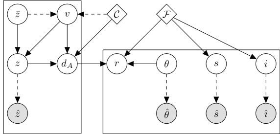
Figure 1: Graphical network showing the structure of the statistical model. Dashed lines show probabilistic relations, while solid lines show deterministic relations, between observed variables (shaded nodes) and latent variables (unshaded nodes). To illustrate the parameter dependence we have distinguished between cosmological parameters $\mathcal{C}$ and parameters related to the FP, $\mathcal{F}=\{a,b,\bar{r},\bar{s},\bar{\imath},\sigma_{1},\sigma_{2},\sigma_{3}\}$. Note that because we are working to first-order precision we can bypass the background redshift $\bar{z}$ altogether by evaluating $v$ at the total redshift $z$.

In the following we derive an analytic expression for the joint posterior for parameters, ignoring for now selection effects; the inclusion of selection effects is discussed in Section 5. We begin by applying Bayes’ theorem to (10):

$$p(\vartheta,\bm{V},\bm{r},\bm{s},\bm{i},\bm{\theta},{\bm{d}}_{A},\bm{z}\mid{\bm{\bm{\hat{z}}}},\bm{\hat{\theta}},\bm{\hat{s}},\bm{\hat{\imath}})\propto p(\hat{\bm{z}},\bm{\hat{\theta}},\bm{\hat{s}},\bm{\hat{\imath}}\mid\vartheta,\bm{V},\bm{r},\bm{s},\bm{i},\bm{\theta},{\bm{d}}_{A},\bm{z})\,p(\vartheta,\bm{V},\bm{r},\bm{s},\bm{i},\bm{\theta},{\bm{d}}_{A},\bm{z}).$$ (12)

The first term on the RHS of (12) is related to the observed data and its experimental errors. Since redshift and angular size measurements are separable from the other observables we can write

$$p(\hat{\bm{z}},\bm{\hat{\theta}},\bm{\hat{s}},\bm{\hat{\imath}}\mid\vartheta,\bm{V},\bm{r},\bm{s},\bm{i},\bm{\theta},{\bm{d}}_{A},\bm{z})=p(\bm{\hat{z}}\mid\bm{z})\,p(\bm{\hat{\theta}}\mid\bm{\theta})\,p(\bm{\hat{s}},\bm{\hat{\imath}}\mid\bm{s},\bm{i}).$$ (13)

For a single object, marginalising over latent variables $z$, $\theta$, $s$, and $i$ in the hierarchical approach is equivalent to convolution of the error distribution with the model (an example of this is (7), which yields (5)). As we show below the marginalisation over $\bm{V}$, $\bm{s}$ and $\bm{i}$ can be performed analytically, while marginalisation over ${\bm{d}}_{A}$ and $\bm{z}$ is straightforward.

The second term on the RHS of (12) is the prior through which the cosmological model enters. This will be the main focus below. We will return to the first term in the end to convolve with the error distribution when we marginalise over $\bm{s}$ and $\bm{i}$.

Now by repeatedly using the chain rule we have

$$p(\vartheta,\bm{V},\bm{r},\bm{s},\bm{i},\bm{\theta},{\bm{d}}_{A},\bm{z}) =p(\bm{r},\bm{s},\bm{i}\mid\vartheta,\bm{V},\bm{\theta},{\bm{d}}_{A},\bm{z})\,p({\bm{d}}_{A}\mid\vartheta,\bm{V},\bm{\theta},\bm{z})\,p(\vartheta,\bm{V},\bm{\theta},\bm{z})$$

$$=p(\bm{r},\bm{s},\bm{i}\mid\vartheta,\bm{\theta},{\bm{d}}_{A})\,p({\bm{d}}_{A}\mid\vartheta,\bm{V},\bm{z})\,p(\bm{V}\mid\bm{z},\vartheta)\,p(\bm{z})\,p(\bm{\theta})\,p(\vartheta),$$ (14)

where in the second line we conditioned only on directly related variables (see Fig. 1).

The fully marginalised posterior to be evaluated is

$$\begin{split}p(\vartheta\mid\bm{\bm{\hat{z}}},\bm{\hat{\theta}},\bm{\hat{s}},\bm{\hat{\imath}})&\propto p(\vartheta)\int\mathrm{d}\bm{V}\,\mathrm{d}\bm{r}\,\mathrm{d}\bm{s}\,\mathrm{d}\bm{i}\,\mathrm{d}{\bm{d}}_{A}\,\mathrm{d}\bm{z}\,\mathrm{d}\bm{\theta}\>\>p(\bm{\hat{z}}\mid\bm{z})\,p(\bm{\hat{\theta}}\mid\bm{\theta})\,p(\bm{\hat{s}},\bm{\hat{\imath}}\mid\bm{s},\bm{i})\\[4.0pt] &\qquad\qquad\times p(\bm{r},\bm{s},\bm{i}\mid\vartheta,\bm{\theta},{\bm{d}}_{A})\,p({\bm{d}}_{A}\mid\vartheta,\bm{V},\bm{z})\,p(\bm{V}\mid\bm{z},\vartheta)\,p(\bm{z})\,p(\bm{\theta}).\end{split}$$ (15)

This integral can be simplified if we note that

$$p({\bm{d}}_{A}\mid\vartheta,\bm{V},\bm{z})=\delta_{D}\big{(}{\bm{d}}_{A}-{\bm{d}}_{A}(\bm{z},\bm{V},\vartheta)\big{)}$$ (16)

and adopt uniform priors $p(\bm{z})=\mathrm{const}$ and $p(\bm{\theta})=\mathrm{const}$. Furthermore, we assume for spectroscopic redshift $\hat{z}$ and angular size $\hat{\theta}$ that errors are negligible (especially compared with the $\sim 20\%$ distance errors), so that we can make the following assignments:

$$p(\bm{\hat{z}}\mid\bm{z}) =\delta_{D}(\bm{\hat{z}}-\bm{z}),$$ (18)

$$p(\bm{\hat{\theta}}\mid\bm{\theta}) =\delta_{D}(\bm{\hat{\theta}}-\bm{\theta}).$$ (19)

However, Gaussian errors on $\hat{z}$ may also be accommodated within this framework with small modification. In this case to perform the marginalisation over $\bm{z}$ analytically we use that the redshift errors are small and linearise the angular diameter distance about $z=\hat{z}$; this was done in the hierarchical model of March et al. (2011), finding that neglecting redshift errors do not have a significant impact on inference.

Absorbing the uniform priors into the proportionality constant and performing three trivial integrations, we are left with the more manageable integral

$$p(\vartheta\mid\bm{\bm{\hat{z}}},\bm{\hat{\theta}},\bm{\hat{s}},\bm{\hat{\imath}})\propto p(\vartheta)\int\mathrm{d}\bm{V}\,\mathrm{d}\bm{r}\,\mathrm{d}\bm{s}\,\mathrm{d}\bm{i}\>\,p\big{(}\bm{r},\bm{s},\bm{i}\mid\vartheta,\bm{\hat{\theta}},{\bm{d}}_{A}(\bm{\hat{z}},\bm{V},\vartheta)\big{)}\,p\big{(}\bm{V}\mid\bm{\hat{z}},\vartheta\big{)}\,p(\bm{\hat{s}},\bm{\hat{\imath}}\mid\bm{s},\bm{i}).$$ (20)

Here we have the integral over the product of three terms. The third term of the integral is the Gaussian error distribution. The other two terms we will manipulate into forms that are readily integrated. In the following sections we show how to analytically perform the rest of the marginalisations over $\bm{V}$, $\bm{r}$, $\bm{s}$, and $\bm{i}$. The basic strategy is to separate out $\bm{r}$ from the joint likelihood using the chain rule. This results in the product of two terms: an $N$-dimensional Gaussian that depends on $\bm{V}$ and a $2N$-dimensional Gaussian that does not. After marginalising over $\bm{V}$ and $\bm{r}$ we rearrange the remaining quadratic forms into a single quadratic form that can be integrated analytically.

3.1 Developing the terms

3.1.1 Fundamental Plane

First we note the probability of obtaining $r$ given $\theta$ and $d_{A}$ is non-zero only when $r=\log\theta+\log d_{A}$; i.e.

$$p(\bm{r},\bm{s},\bm{i}\mid\vartheta,\bm{\hat{\theta}},{\bm{d}}_{A})=p(\bm{r},\bm{s},\bm{i}\mid\vartheta,\bm{\hat{\theta}},{\bm{d}}_{A})\,\delta_{D}\big{(}\bm{r}-\bm{L_{\theta}}-\bm{L_{d}}\big{)},$$ (21)

where we defined

$$\bm{L_{\theta}}\equiv\big{(}\log\hat{\theta}_{1},\log\hat{\theta}_{2},\ldots,\log\hat{\theta}_{N}\big{)}^{\mathsf{T}},$$ (22a)

$$\bm{L_{d}}\equiv\big{(}\log d_{A}(\hat{z}_{1}),\log d_{A}(\hat{z}_{2}),\ldots,\log d_{A}(\hat{z}_{N})\big{)}^{\mathsf{T}}.$$ (22b)

Marginalisation over $\bm{r}$ results in the replacement of $\bm{r}$ with $\bm{L_{\theta}}+\bm{L_{d}}$.

Now, recall that for a single object the FP properties $r,s,i$ are independently and identically drawn from same underlying population model (5):

$$r,s,i\sim\mathcal{N}\big{(}(\bar{r},\bar{s},\bar{\imath}),\mathbf{C}^{\mathrm{FP}}\big{)}.$$ (23)

The individual likelihood $p(r,s,i\mid\vartheta,\theta,d_{A})$ is therefore a trivariate Gaussian with mean $(\bar{r},\bar{s},\bar{\imath})^{\mathsf{T}}$ and covariance $\mathbf{C}^{\mathrm{FP}}={\mathbf{O}}{\mathbf{D}}{\mathbf{O}}^{\mathsf{T}}$. While the joint likelihood (6) can be written as the product of $N$ trivariate Gaussians, to facilitate integration we will instead form a $3N$-dimensional multivariate Gaussian for which the first $N$ rows and columns correspond to $\bm{r}$, the next $N$ correspond to $\bm{s}$, and the last $N$ correspond to $\bm{i}$. In particular

$$\bm{r},\bm{s},\bm{i}\sim\mathcal{N}\big{(}(\bm{\bar{r}},\bm{\bar{s}},\bm{\bar{\imath}}),\mathring{\mathbf{C}}\big{)},$$ (24)

where the joint covariance is partitioned in block form as

$$\mathring{\mathbf{C}}\equiv\begin{pmatrix}\mathbf{C_{rr}}&\mathbf{M}^{\mathsf{T}}\\ \mathbf{M}&\mathbf{C_{yy}}\end{pmatrix}.$$ (25)

Here $\mathbf{C_{rr}}$ is a $N\times N$ matrix, $\mathbf{M}$ is a $2N\times N$ matrix, and $\mathbf{C_{yy}}$ is a $2N\times 2N$ matrix. In this way, when conditioning on $\bm{s}$ and $\bm{i}$, we may use the formulae of Appendix B.1. Since we will be marginalising over $\bm{V}$ we require the conditional form

$$p(\bm{r},\bm{s},\bm{i}\mid\vartheta,\bm{\theta},{\bm{d}}_{A})=p(\bm{r}\mid\bm{s},\bm{i},\vartheta,\bm{\theta},{\bm{d}}_{A})\,p(\bm{s},\bm{i}\mid\vartheta),$$ (26)

where we have dropped the conditioning on $\bm{\theta}$ and ${\bm{d}}_{A}$ in the second term. The first term is

$$p(\bm{r}\mid\bm{s},\bm{i},\vartheta,\bm{\theta},{\bm{d}}_{A})=\mathcal{N}(\bm{r}\,;\,\bm{\bar{r}}^{\prime},\mathbf{C_{rr}}^{\prime})$$ (27)

with (see Appendix B.1)

$$\bm{\bar{r}}^{\prime}=\bm{\bar{r}}-\mathbf{M}^{\mathsf{T}}\,\mathbf{C}_{\mathbf{yy}}^{-1}\,(\mathbf{\bar{y}}-\mathbf{y}),$$ (28a)

$$\mathbf{C_{rr}}^{\prime}=\mathbf{C_{rr}}-\mathbf{M}^{\mathsf{T}}\,\mathbf{C}_{\mathbf{yy}}^{-1}\,\mathbf{M},$$ (28b)

where $\mathbf{y}\equiv(\bm{s},\bm{i})^{\mathsf{T}}$ and $\mathbf{\bar{y}}\equiv(\bm{\bar{s}},\bm{\bar{\imath}})^{\mathsf{T}}$ are $2N$-dimensional vectors. The second term of (26) is given by a higher-dimensional analog of (5), marginalised over $\bm{r}$ (i.e. striking out the first $N$ rows and columns):

$$p(\bm{s},\bm{i}\mid\vartheta)=\mathcal{N}(\mathbf{y}\,;\,\mathbf{\bar{y}},\mathbf{C_{yy}}).$$ (29)

Altogether we have

$$p(\bm{r},\bm{s},\bm{i}\mid\vartheta,\bm{\hat{\theta}},{\bm{d}}_{A})=\mathcal{N}(\bm{r}\,;\,\bm{\bar{r}}^{\prime},\mathbf{C_{rr}}^{\prime})\,\mathcal{N}(\mathbf{y}\,;\,\mathbf{\bar{y}},\mathbf{C_{yy}})\,\delta_{D}\big{(}\bm{r}-\bm{L_{\theta}}-\bm{L_{d}}\big{)}.$$ (30)

Finally we have for the error distribution

$$p(\bm{\hat{s}},\bm{\hat{\imath}}\mid\bm{s},\bm{i})=\mathcal{N}(\mathbf{\hat{y}}\,;\,\mathbf{y},\mathbf{E_{yy}}),$$ (31)

where $\mathbf{E_{yy}}$ is constructed in a similar way to $\mathbf{C_{yy}}$ of (25).

3.1.2 Distance-redshift relation

At the low redshifts typical of a peculiar velocity catalogue the angular diameter distance is given by (see Hui & Greene (2006); for a direct calculation see Kaiser & Hudson (2015))

$$d_{A}(z)=\bar{d}_{A}(z)(1-\kappa),\qquad\kappa(z)=\left[1-\frac{d_{H}(z)}{\bar{d}_{A}(z)}\right]\frac{v}{c},$$ (32)

where $d_{H}(z)=c/H(z)$ and all terms are evaluated at the total redshift $z=\hat{z}$. It is in this regime that the dominant contribution to the convergence $\kappa$ is from peculiar velocity. Since $v/c\sim 10^{-3}$ we have $\kappa\lesssim 0.1$ for $z\gtrsim 0.01$, and we therefore approximate $\ln(1-x)\simeq-x$, as in Adams & Blake (2017), and write

$$\log d_{A}(z)\simeq\log\bar{d}_{A}(z)-\frac{\kappa(z)}{\ln 10},$$ (33)

or in vector form

$$\bm{L_{d}}=\bm{L_{\bar{d}}}+\mathbf{A}\bm{V},$$ (34)

where we defined $\bm{L_{\bar{d}}}=\big{(}\log\bar{d}_{A}(\hat{z}_{1}),\log\bar{d}_{A}(\hat{z}_{2}),\ldots,\log\bar{d}_{A}(\hat{z}_{N})\big{)}^{\mathsf{T}}$ and the $N\times N$ symmetric matrix

$$\mathbf{A}=\mathrm{diag}(A_{1},A_{2},\ldots,A_{N}),\qquad A_{m}=\frac{1}{c\ln 10}\left[\frac{d_{H}(\hat{z}_{m})}{\bar{d}_{A}(\hat{z}_{m})}-1\right],$$ (35)

and we note that $A_{m}\sim 1/z_{m}$ at low redshifts, and is why the fluctuations to the distance can be large.

3.1.3 Large-scale structure

As well as the usual distance-redshift relation, cosmology also enters through correlations in the source velocities. Because neighbouring sources will move with similar velocity, we expect correlations between source pairs meaning the PDF of $\bm{V}$ will not be separable. In linear theory, the joint peculiar velocity distribution is described by a multivariate Gaussian

$$p(\bm{V}\mid\bm{z},\vartheta)=\mathcal{N}(\bm{V}\,;\,\bm{0},\mathbf{R})=\frac{1}{\det(2\pi\mathbf{R})^{1/2}}\exp\left(-\frac{1}{2}\bm{V}^{\mathsf{T}}\mathbf{R}^{-1}\bm{V}\right).$$ (36)

Here the prior of $\bm{V}$ is taken to be the likelihood in the standard analysis taken over the catalogue data (e.g. Jaffe & Kaiser (1995); Ma, Gordon & Feldman (2011); Macauley et al. (2012); Johnson et al. (2014)). Depending on the model under consideration other choices of prior are possible. However, for the current discussion we will focus on a spatially flat $\Lambda$CDM cosmology. The covariance between the $m^{\mathrm{th}}$ and $n^{\mathrm{th}}$ source is given by

$$R_{mn}=\big{\langle}v(\bm{x}_{m})\,v(\bm{x}_{n})\big{\rangle}=\xi_{v}(\bm{x}_{m},\bm{x}_{n}),$$ (37)

where $\xi_{v}$ is the two-point correlation function of the LOS velocities. The $m^{\mathrm{th}}$ source has a redshift-space position of $(z_{m},\alpha_{m},\delta_{m})$, or in real-space $\bm{x}_{m}=D_{m}\,\hat{\bm{n}}_{m}$, with $D_{m}\equiv D(z_{m})$ the comoving distance and $\hat{\bm{n}}_{m}=\hat{\bm{n}}(\alpha_{m},\delta_{m})$ the direction of observation. Notice that we set the galaxy distance at their observed redshift $z$, and not the background redshift $\bar{z}$, corresponding to the real-space position. Just like redshift-space density fluctuations, peculiar velocities are also affected by redshift-space distortions; however, in linear theory the real-space and redshift-space velocity correlation functions are equivalent (Koda et al., 2014; Okumura et al., 2014). We reiterate that in this work we only demonstrate a template analysis from which we can develop more sophisticated models.

On subhorizon scales, typical of peculiar velocity surveys, we can use the linearised continuity equation ${\delta^{\prime}+\nabla\cdot\bm{v}=0}$ so that the correlation function can be expressed in terms of the matter power spectrum. For production work, the correlation function is better formulated in terms of the velocity divergence $\nabla\cdot\bm{v}$ because it does not manifestly depend on the linearised continuity equation and require a galaxy bias model; non-linear corrections are also more easily implemented (Johnson et al., 2014). The correlation function reads

$$\xi_{v}(\bm{x}_{m},\bm{x}_{n})=\frac{1}{2\pi^{2}}\,f^{2}_{0}\,H_{0}^{2}\int{\mathrm{d}k}\,W_{mn}(k)P(k),$$ (38)

where, at the low redshifts typical of peculiar velocity surveys, we have made the usual assumption about equal-time correlations; $f_{0}\equiv f(a_{0})$ is the present-day growth rate, with $f_{0}\approx\Omega_{m}^{\gamma}$, and $\gamma\approx 0.55$ for $\Lambda$CDM. We have also the matter power spectrum $P(k)$, and the window function

$$W_{mn}(k) \equiv\int\frac{\mathrm{d}^{2}{\hat{\bm{k}}}}{4\pi}\,e^{-ik\hat{\bm{k}}\cdot(\bm{x}_{m}-\bm{x}_{n})}(\hat{\bm{k}}\cdot\hat{\bm{n}}_{m})(\hat{\bm{k}}\cdot\hat{\bm{n}}_{n})$$

$$=\frac{1}{3}\big{[}j_{0}(kr_{mn})-2j_{2}(kr_{mn})\big{]}\cos\Upsilon_{mn}+\frac{D_{m}D_{n}}{r_{mn}^{2}}j_{2}(kr_{mn})\sin^{2}\Upsilon_{mn}.$$ (39)

Here $r^{2}_{mn}=|\bm{x}_{m}-\bm{x}_{n}|^{2}=D^{2}_{m}+D^{2}_{n}-2D_{m}D_{n}\cos\Upsilon_{mn}$ by the cosine rule, and $\Upsilon_{mn}=\arccos(\hat{\bm{n}}_{m}\cdot\hat{\bm{n}}_{n})$ is the angular separation between the $m^{\mathrm{th}}$ and $n^{\mathrm{th}}$ object; $j_{0}$ and $j_{2}$ are the zeroth and second order spherical Bessel functions, respectively. The second line is expressed in terms of observer-centric quantities [see Ma, Gordon & Feldman (2011) for a derivation]; it is equivalent to the more common decomposition in terms of parallel and perpendicular kernels (see, e.g. Peebles (1993)).

It is also necessary to include in $\mathbf{R}$ a velocity dispersion $\sigma^{2}_{*}$ so that $R_{mn}\to R_{mn}+\sigma^{2}_{*}\,\delta_{mn}$ in which $\sigma_{*}$ is treated as a free parameter included in $\vartheta$. This parameter captures the one-dimensional incoherent Gaussian random motion of galaxies on non-linear scales. We remark that there is a slight difference with the usual approach, which is that here $v_{m}$ are the latent radial velocities so have no catalogue error.

3.2 Marginalisation

After inserting (30), (34), and (36) into (20) and rearranging slightly, the posterior reads

$$\begin{split}p(\vartheta\mid\bm{\bm{\hat{z}}},\bm{\hat{\theta}},\bm{\hat{s}},\bm{\hat{\imath}})\propto p(\vartheta)&\int\mathrm{d}\mathbf{y}\>\mathcal{N}(\mathbf{\hat{y}}\,;\,\mathbf{y},\mathbf{E_{yy}})\,\mathcal{N}(\mathbf{y}\,;\,\mathbf{\bar{y}},\mathbf{C_{yy}})\\ &\times\int\mathrm{d}\bm{V}\int\mathrm{d}\bm{r}\>\mathcal{N}(\bm{r}\,;\,\bm{\bar{r}}^{\prime},\mathbf{C_{rr}}^{\prime})\,\delta_{D}\big{(}\bm{r}-\bm{L_{\theta}}-\bm{L_{\bar{d}}}-\mathbf{A}\bm{V}\big{)}\,\mathcal{N}(\bm{V}\,;\,\bm{0},\mathbf{R}).\end{split}$$ (40)

Integrating out $\bm{r}$ is trivial because of the delta function, and gives

$$\begin{split}p(\vartheta\mid\bm{\bm{\hat{z}}},\bm{\hat{\theta}},\bm{\hat{s}},\bm{\hat{\imath}})\propto p(\vartheta)&\int\mathrm{d}\mathbf{y}\>\mathcal{N}(\mathbf{\hat{y}}\,;\,\mathbf{y},\mathbf{E_{yy}})\,\mathcal{N}(\mathbf{y}\,;\,\mathbf{\bar{y}},\mathbf{C_{yy}})\\ &\times\int\mathrm{d}\bm{V}\>\mathcal{N}\big{(}\bm{\bar{r}}^{\prime}\,;\,\bm{r}(\bm{L_{\theta}},\bm{L_{\bar{d}}},\mathbf{A}\bm{V},\vartheta),\mathbf{C_{rr}}^{\prime}\big{)}\,\mathcal{N}(\bm{V}\,;\,\bm{0},\mathbf{R}),\end{split}$$ (41)

where $\bm{r}(\bm{L_{\theta}},\bm{L_{\bar{d}}},\mathbf{A}\bm{V},\vartheta)=\bm{L_{\theta}}+\bm{L_{\bar{d}}}+\mathbf{A}\bm{V}$. The above expression can be thought of as a double convolution: the first convolves the distance-dependent part of the FP (for a given distance-redshift relation) with the peculiar velocity distribution due to correlations from large-scale structure and cosmic variance; the second convolution is with the distance-independent part of the FP. Note that the two integrals cannot be separated because $\bm{\bar{r}}^{\prime}$ depends on $\mathbf{y}$ by (28a).

With a change of variables $\bm{V}\to\bm{U}=\mathbf{A}\bm{V}$ the inner $\bm{V}$ integral of (41) is readily performed using (67) to give

$$p(\vartheta\mid\bm{\bm{\hat{z}}},\bm{\hat{\theta}},\bm{\hat{s}},\bm{\hat{\imath}})\propto p(\vartheta) \int\mathrm{d}\mathbf{y}\>\mathcal{N}(\mathbf{\hat{y}}\,;\,\mathbf{y},\mathbf{E_{yy}})\,\mathcal{N}(\mathbf{y}\,;\,\mathbf{\bar{y}},\mathbf{C_{yy}})\,\mathcal{N}(\bm{\Delta}_{r}\,;\,\bm{0},\mathbf{\Sigma_{rr}}),$$ (42)

where we defined

$$\bm{\Delta}_{r}\equiv\bm{\bar{r}}^{\prime}-\bm{L_{\theta}}-\bm{L_{\bar{d}}}=\big{[}\bm{\bar{r}}-\mathbf{M}^{\mathsf{T}}\,\mathbf{C}_{\mathbf{yy}}^{-1}\,(\mathbf{\bar{y}}-\mathbf{y})\big{]}-\big{(}\bm{L_{\theta}}+\bm{L_{\bar{d}}}\big{)},$$ (43a)

$$\mathbf{\Sigma_{rr}}\equiv\mathbf{A}\mathbf{R}\mathbf{A}+\mathbf{C_{rr}}^{\prime}=\mathbf{A}\mathbf{R}\mathbf{A}+\mathbf{C_{rr}}-\mathbf{M}^{\mathsf{T}}\,\mathbf{C}_{\mathbf{yy}}^{-1}\,\mathbf{M}\,.$$ (43b)

This leaves us with one final integral, which can be done by bringing the integrand into Gaussian canonical form then using (70). The details of this calculation are given in Appendix C; here we state only the final result:

$$p(\vartheta\mid\bm{\hat{z}},\bm{\hat{\theta}},\bm{\hat{s}},\bm{\hat{\imath}})\propto\frac{1}{\det\mathbf{\Sigma}^{1/2}}\bigg{[}\prod_{m=1}^{N}\frac{1}{\det(\mathbf{C}+\mathbf{E}_{m})^{1/2}}\bigg{]}\exp\bigg{[}-\frac{1}{2}\bm{\Delta}^{\mathsf{T}}\,\mathbf{\Sigma}^{-1}\,\bm{\Delta}-\frac{1}{2}\sum_{m=1}^{N}\Delta\mathbf{y}_{m}^{\mathsf{T}}\,(\mathbf{C}+\mathbf{E}_{m})^{-1}\,\Delta\mathbf{y}_{m}\bigg{]}\,p(\vartheta),$$ (44)

where

$$\bm{\Delta} =\big{[}\bm{\bar{r}}-\mathbf{M}^{\mathsf{T}}\,(\mathbf{C_{yy}}+\mathbf{E_{yy}})^{-1}\,(\mathbf{\bar{y}}-\mathbf{\hat{y}})\big{]}-(\bm{L_{\theta}}+\bm{L_{\bar{d}}}),$$ (45a)

$$\mathbf{\Sigma} =\mathbf{A}\mathbf{R}\mathbf{A}+\mathbf{C_{rr}}-\mathbf{M}^{\mathsf{T}}\,(\mathbf{C_{yy}}+\mathbf{E_{yy}})^{-1}\,\mathbf{M}.$$ (45b)

and $\Delta\mathbf{y}_{m}=(\hat{s}_{m}-\bar{s},\hat{\imath}_{m}-\bar{\imath})^{\mathsf{T}}$, with $\mathbf{C}$ and $\mathbf{E}_{m}$ being the corresponding $2\times 2$ submatrices of $\mathbf{C}^{\mathrm{FP}}$ and $\mathbf{E}^{\mathrm{FP}}_{m}$, respectively. It can be seen that the joint posterior density is composed of two Gaussian densities (that we have written into a single exponential): The first is cosmological in nature, accounting for the distance-redshift relation and cosmic variance; the second is purely related to the physical characteristics of galaxies. Notice that the presence of $\mathbf{R}$ correlates all galaxies; this is in contrast to the conventional analysis, which considers only correlations from the FP. Here $\mathbf{\Sigma}$ is a dense matrix because of the presence of $\mathbf{A}\mathbf{R}\mathbf{A}$; the first quadratic form in the exponential of (44) cannot be reduced down to the product of smaller terms. By comparison the physical properties of each galaxy (velocity dispersion and surface brightness) being independent of one another allows us to write the $2N\times 2N$ quadratic form of $\mathbf{\hat{y}}$ as the sum of $N$ $2\times 2$ quadratic forms, c.f. (7).

Except for $\mathbf{E_{yy}}$, note that all matrices depend on parameters so that the determinants must be included in any parameter scans. We further emphasize $\bm{L_{\bar{d}}}$ also depends on parameters through the angular diameter distance.

Aside from the factors of $2\pi$ we have omitted, the proportionality also accounts for prior on $\bm{\bar{z}}$, which is unimportant for parameter estimation when the uncertainties are assumed to be negligible.

3.3 Recovering the Fundamental Plane likelihood

As a consistency check, we verify that the standard FP likelihood (5) can be recovered if we fix the cosmological parameters and take $\mathbf{R}\to 0$ (no correlations from large-scale structure). Now, as the mapping from distance to physical size is fully determined by the (known) cosmological parameters, we can swap the observables $\bm{L_{\theta}}$ and $\bm{L_{\bar{d}}}$ with the conventional size observable defined as $\bm{\bm{\hat{}}{r}}\equiv\bm{L_{\theta}}+\bm{L_{\bar{d}}}$. We thus have $\bm{\Delta}=\bm{\bar{r}}^{\prime}-\bm{\bm{\hat{}}{r}}$, with $\bm{\bar{r}}^{\prime}\equiv\bm{\bar{r}}-\mathbf{M}^{\mathsf{T}}(\mathbf{C_{yy}}+\mathbf{E_{yy}})^{-1}(\mathbf{\bar{y}}-\mathbf{\hat{y}})$ the shifted mean. This recovers (5) in conditional form

$$p(\vartheta\mid\bm{\bm{\hat{}}{r}},\bm{\hat{s}},\bm{\hat{\imath}}) \propto\frac{1}{\det\mathbf{\Sigma}^{1/2}}\exp\left[-\frac{1}{2}(\bm{\bar{r}}^{\prime}-\bm{\bm{\hat{}}{r}})^{\mathsf{T}}\,\mathbf{\Sigma}^{-1}\,(\bm{\bar{r}}^{\prime}-\bm{\bm{\hat{}}{r}})\right]\prod_{m=1}^{N}\frac{1}{\det(\mathbf{C}+\mathbf{E}_{m})^{1/2}}\exp\left[-\frac{1}{2}\Delta\mathbf{y}_{m}^{\mathsf{T}}\,(\mathbf{C}+\mathbf{E}_{m})^{-1}\,\Delta\mathbf{y}_{m}\right].$$ (47)

Without correlations induced by $\mathbf{R}$ we have that $\mathbf{\Sigma}=\mathbf{C_{rr}}-\mathbf{M}^{\mathsf{T}}\,(\mathbf{C_{yy}}+\mathbf{E_{yy}})^{-1}\,\mathbf{M}$ is a diagonal matrix, allowing the first two terms to be factorised into a product of $N$ univariate Gaussians. The resulting expression can thus be manipulated into the form of the product of $N$ trivariate Gaussians.

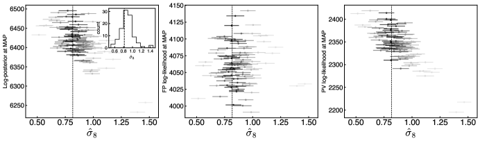
Figure 2: Maximum a posterior estimates of $\sigma_{8}$ from 100 FP mock data realisations of $N=1000$ galaxies and plotted against the value of the logarithm of the likelihood or posterior. As a crude estimate of the uncertainty we also show the associated Hessian errors of $\sigma_{8}$. The gray-scale indicates the RMS difference from the true value $\sigma_{8}=0.817$ (dashed line), with the darkest having the smallest RMS and lightest the largest. Note the difference between the sum of the FP and peculiar velocity log-likelihoods and the log-posterior is because of the log-uniform priors we assign to the scale parameters $\sigma_{1}$, $\sigma_{2}$, $\sigma_{3}$, and $\sigma_{8}$; all other parameters are assigned uniform priors.

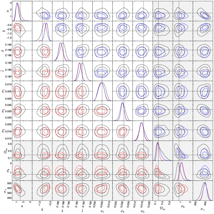
Figure 3: The marginalised posteriors when (i) $\bar{r}$ is free to vary (black curves), (ii) the calibration is fixed to a value $10\%$ lower than the true value $\bar{r}=0.191$ (blue curves), and (iii) the calibration is fixed to a value $10\%$ higher than the true value (red curves). Note in each case all other calibration parameters are fitted for. The true values are indicated by dashed black lines. Particular attention should be paid to joint contours between cosmological and FP parameters (highlighted in grey), where calibration parameters fixed to wrong values can potentially lead to systematic shifts in the parameters of interest. These constraints should not be viewed as indicative of the performance on realistic data sets as here we fit to a small sample of galaxies ($N=1000$) and assume $1\%$ statistical errors on $\hat{s}$ and $\hat{\imath}$. Here $\sigma_{*}$ is in units $\mathrm{km/s}$ and is not known a priori.

3.4 Fundamental Plane calibration uncertainty

Another advantage of our unified treatment is that the uncertainty in FP calibration parameters can be straightforwardly propagated downstream to the cosmological parameters. Although we have left the nuisance parameters (i.e. FP parameters) unmarginalised, the centroid parameters $\bar{r}$, $\bar{s}$, and $\bar{\imath}$ can in fact be analytically marginalised over if we assume Gaussian priors. For example, carrying out the marginalisation assuming a Gaussian prior on $\bar{r}$ with mean $\mu_{\bar{r}}$ and variance $\sigma^{2}_{\bar{r}}$, the final result is a modified form of (44) with $\bm{\bm{\bar{r}}}=\bar{r}{\mathbf{1}}\to\mu_{\bar{r}}{\mathbf{1}}$, and a monopole contribution to the covariance, $\mathbf{\Sigma_{rr}}\to\mathbf{\Sigma_{rr}}+\sigma_{\bar{r}}^{2}\,{\mathbf{J}}_{N}$, where ${\mathbf{J}}_{N}$ is the $N\times N$ matrix of ones (Bridle et al., 2002). This shows that uncertainty in global parameters like $\bar{r}$ induces an ambient error and covariance for all objects.

We note that we can also analytically marginalise over $\bar{s}$ and $\bar{\imath}$ in a similar way, but that the parameters $a$ and $b$ enter into the covariance matrices so will have to be marginalised over by other means.

3.5 Maximum a posteriori estimator for peculiar velocities

The posterior (44) derived is marginalised over all peculiar velocities. However, if we leave $\bm{V}$ unmarginalised then we would have an expression for $p(\vartheta,\bm{V}\mid\mathscr{D})$, with $\mathscr{D}=\{\bm{\hat{z}},\bm{\hat{\theta}},\bm{\hat{s}},\bm{\hat{\imath}}\}$, and the posterior for $\bm{V}$ is

$$p(\bm{V}\mid\mathscr{D})=\int\mathrm{d}\vartheta\,p(\vartheta,\bm{V}\mid\mathscr{D}).$$ (48)

Building probabilistic peculiar velocity catalogues from (48) would be desirable from a Bayesian perspective as any uncertainty in the calibration and cosmology is accounted for (Brewer, Foreman-Mackey & Hogg, 2013; Portillo et al., 2017). The problem, however, is that (48) is a high-dimensional posterior and standard MCMC methods are unfeasible for realistic data sets containing $N\gtrsim 10^{4}$ galaxies and clusters, though Gibbs sampling can be effective provided the conditional distributions of the target posterior have a simple form. An alternative is to construct point estimators for $\bm{V}$. Since the prior on $\bm{V}$ is a multivariate Gaussian the joint posterior containing $\bm{V}$ is the product of two Gaussians. It is straightforward to solve ${\partial p(\vartheta,\bm{V}\mid\mathscr{D})/\partial\bm{V}=0}$ for $\bm{V}$ to obtain the maximum a posteriori (MAP) estimate

$$\widehat{\bm{V}}_{\mathrm{MAP}}=\mathbf{R}\mathbf{A}\mathbf{\Sigma}^{-1}\bm{\Delta}.$$ (49)

Manipulating this slightly, the estimator can be seen to be equivalent to the Wiener filtering of the residuals $\mathbf{A}^{-1}\bm{\Delta}$:

$$\widehat{\bm{V}}_{\mathrm{MAP}}=\big{[}\mathbf{R}(\mathbf{R}+\mathbf{A}^{-1}\mathbf{\Sigma}_{0}\mathbf{A}^{-1})^{-1}\big{]}\mathbf{A}^{-1}\bm{\Delta}.$$ (50)

where $\mathbf{\Sigma}_{0}\equiv\mathbf{C_{rr}}-\mathbf{M}^{\mathsf{T}}\,(\mathbf{C_{yy}}+\mathbf{E_{yy}})^{-1}\,\mathbf{M}$, which differs from $\mathbf{\Sigma}$ by $\mathbf{A}\mathbf{R}\mathbf{A}$, and the term in square brackets is the linear optimal filter with signal $\mathbf{R}$ and noise $\mathbf{A}^{-1}\mathbf{\Sigma}_{0}\mathbf{A}^{-1}$. The associated covariance of the MAP estimate is given by the inverse of the Hessian of the log-posterior:

$$\widehat{\mathbf{C}}_{\mathrm{MAP}}=(\mathbf{R}^{-1}+\mathbf{A}\mathbf{\Sigma}_{0}^{-1}\mathbf{A})^{-1}.$$ (51)

As discussed in Section 3.4, uncertainty in the calibration parameters can be built into the estimate. If we are uncertain about the zero-point (i.e. $\bar{r}$) by $\sigma_{\mathrm{ZP}}$, then we have the slight modification

$$\widehat{\mathbf{C}}_{\mathrm{MAP}}=\big{[}\mathbf{R}^{-1}+\mathbf{A}(\sigma^{2}_{\mathrm{ZP}}\,{\mathbf{J}}_{N}+\mathbf{\Sigma}_{0})^{-1}\mathbf{A}\big{]}^{-1},$$ (52)

where ${\mathbf{J}}_{N}$ is the $N\times N$ matrix of ones.

4 Numerical experiments

As a proof of concept, we analyse mock data with the aim of recovering the true parameters given some measurement error. Recall we require the following data:

$$\mathscr{D}=\Big{\{}\big{(}\hat{z}_{m},\,\hat{\theta}_{m},\,\hat{s}_{m},\,\hat{\imath}_{m},\,\hat{\alpha}_{m},\,\hat{\delta}_{m}\big{)}\Big{\}}_{m=1}^{N}.$$ (53)

The positions and peculiar velocities of the galaxies are fixed according to a halo catalogue we obtain from the Big MultiDark Planck $N$-body simulation (BigMDPL) (Klypin et al., 2016). BigMDPL is a dark matter only simulation performed using the l-gadget-2 code (Springel, 2005). The simulation box has a side length of $2.5h^{-1}\,\mathrm{Gpc}$, a mass resolution of $2.4\times 10^{10}h^{-1}\,M_{\odot}$, and consists of $3840^{3}$ particles, which are evolved forward from an initial redshift of $z=100$. The simulation assumes a spatially flat $\Lambda$CDM cosmology with $h=0.678$, $\Omega_{m}=0.307$, $\Omega_{\Lambda}=0.693$, $\Omega_{b}=0.048$, $n_{s}=0.96$, and $\sigma_{8}=0.829$. We use the halo catalogue derived from the $z=0$ snapshot, which was constructed using the rockstar halo finder (Behroozi, Wechsler & Wu, 2013). Halos are selected in the mass range of ${10^{11.5}-10^{12}}h^{-1}\,M_{\odot}$. Simulation data is obtained from the CosmoSim online database.

The FP data are generated using $a=1.502$, $b=-0.877$, $\bar{r}=0.191$, $\bar{s}=2.188$, $\bar{\imath}=3.184$, $\sigma_{1}=0.0052$, $\sigma_{2}=0.0315$, and $\sigma_{3}=0.0169$. In addition we also include the free parameter $\sigma_{*}$ to capture the small scale random motions not described by linear theory. In all fits we fix $n_{s}$, $h$, and $\Omega_{b}$ to their true values.

We draw $N=1000$ triples $(r_{m},s_{m},i_{m})$ from the intrinsic population given by the trivariate Gaussian with mean $\mathbf{\bar{x}}$ and covariance $\mathbf{C}$, i.e. $\mathbf{x}_{m}\sim\mathcal{N}(\mathbf{\bar{x}},\mathbf{C})$. The selection criteria of our halo catalogue is chosen so that it follows a 6dFGS-like distribution of galaxies (Campbell et al., 2014). Thus sky positions will be located in one hemisphere relative to an observer placed in the centre of the simulation box. The redshift distribution is chosen such that number density is approximately constant, so the differential number density is $(\mathrm{d}n/\mathrm{d}z)\,\mathrm{d}z\propto z^{2}\,\mathrm{d}z$ in the range $z$ to $z+\mathrm{d}z$, and bounded by $z_{\mathrm{min}}=0.006$ and $z_{\mathrm{max}}=0.05$. The observed redshift $z_{m}$ is computed from $z_{m}=(1+\bar{z}_{m})(1+v_{m}/c)-1$, with $\bar{z}_{m}$ obtained from the comoving position and $v_{m}$ taken directly from the halo catalogue. The perturbed angular diameter distance $d_{A}$ as a function of the observed redshift $z_{m}$ and peculiar velocity $v_{m}$ is computed using (32), giving an angular size of $\theta_{m}=10^{r_{m}}/d_{A}(z_{m})$.

Our choice of analysing a relatively small number of galaxies is made for reasons of speed. Realistic FP samples have $N\gtrsim 10^{4}$, requiring the inversion of matrices of size $N\times N$, which is a significant computational cost. For analyses of real data, a practical solution is to use a gridding method (Abate et al., 2008; Johnson et al., 2014) as a form of dimensional reduction; here, as a concession to the small sample size, we will take slightly more optimistic measurement errors instead. The errors $\epsilon_{s,m}$ and $\epsilon_{i,m}$ will thus be drawn from a Gaussian with a standard deviation equal to $1\%$ of the values of $s_{m}$ and $i_{m}$ so that we take as observed quantities $\hat{s}_{m}=s_{m}+\epsilon_{s,m}$ and $\hat{\imath}_{m}=i_{m}+\epsilon_{i,m}$. (For comparison, 6dF galaxy survey errors on $\hat{\imath}$ in $J$ band and $\hat{s}$ are around the $2-3\%$ level.)

Since $a$, $b$, and $c$ have non-trivial correlations, we performed the sampling in the space of FP centroids $\mathbf{\bar{x}}=(\bar{r},\bar{s},\bar{\imath})^{\mathsf{T}}$ and $3\times 3$ covariance matrices $\mathbf{C}^{\mathrm{FP}}$ parametrized by $\sigma_{r}$, $\sigma_{s}$, $\sigma_{i}$, and the correlation coefficients $\rho_{rs}$, $\rho_{ri}$, $\rho_{si}$. These parameters are generally less correlated and better sampling behaviour. Note there is one additional free parameter than in the standard FP fit and this corresponds to the freedom to rotate the FP on to itself, without changing $a$ and $b$. While this does not change the FP relation, allowing for this rotation does change the quality of fit; here we do not fix this degree of freedom. The FP orientation parameters $a$ and $b$ are derived from the MCMC chains as a post-processing step. These are obtained by computing the eigenvector $\bm{e}_{1}=(A,B,C)^{\mathsf{T}}$ of $\mathbf{C}^{\mathrm{FP}}$ with the lowest eigenvalue. This corresponds to the direction with lowest variances and defines the FP; FP relation parameters are then given by $a=-B/A$ and $b=-C/A$ (see Appendix A). Moreover, the parameters $\sigma_{1}$, $\sigma_{2}$, and $\sigma_{3}$ can be computed by taking the square root of the eigenvalues of $\mathbf{C}^{\mathrm{FP}}$.

We assign uninformative priors that are flat in $\ln\sigma_{1}$, $\ln\sigma_{2}$, $\ln\sigma_{3}$, $\rho_{rs}$, $\rho_{ri}$, $\rho_{si}$, $\bar{r}$, $\bar{s}$, $\bar{\imath}$, $\Omega_{m}$, $\ln\sigma_{8}$, and $\ln\sigma_{*}$; the correlation coefficients are bounded by $-1$ and $1$, while $\Omega_{m}$ is bounded by 0 and 1. The posterior distribution is sampled using an affine-invariant ensemble MCMC scheme (Foreman-Mackey et al., 2013).

In Fig. 2 we show the robustness of $\hat{\sigma}_{8}$ for 100 different data realisations. Note that peculiar velocities are generated independent of the FP (latent) data $\bm{r},\bm{s},\bm{i}$. The fact that the recovered $\hat{\sigma}_{8}$ departs from the true value is not because of the FP data but the particular peculiar velocity sample drawn; for a highly dispersive sample $\hat{\sigma}_{8}$ is larger than the true value (lower values of the peculiar velocity likelihood), while it is smaller for a sample drawn near the centroid (higher values of the peculiar velocity likelihood.

In Fig. 3 we show the estimated parameters from one realisation of the ersatz data set with $N=1000$ galaxies and $1\%$ errors on the measured $\hat{s}$ and $\hat{\imath}$. Though these errors are optimistic – realistically we can expect $\gtrsim 2\%$ from current catalogues – we are analysing a much smaller data set. Also shown is the impact when the zero-point, $\bar{r}$, or equivalently $c$, is fixed. Note in the joint fit ($\bar{r}$ free) we find $0.194^{+0.006}_{-0.010}$ ($68\%$ C.L), very much consistent with the true value. As expected, the overconfidence can be seen to produce tighter constraints, but can also cause a systematic shift in other parameters when $\bar{r}$ is fixed away from the mode (i.e. $\bar{r}$ is biased). This is most apparent for $\sigma_{8}$ when $\bar{r}$ is biased $\pm 10\%$ from the true value. In the case when $\bar{r}$ is a free parameter the constraint on $\Omega_{m}$ is considerably degraded; furthermore, the constraint on $\Omega_{m}$ when $\bar{r}$ is biased high is noticeably stronger than when it is biased low. To some extent the zero-point marginalisation procedure of Johnson et al. (2014) performed post-calibration offsets some of this bias, but assumes the marginal posterior of $\bar{r}$ is exactly Gaussian. The above asymmetric constraints and biases suggests this can only be a first approximation. The difference with our consistent marginalisation will be further investigated in future work.

5 Selection effects

The likelihood (44) derived above applies in an idealised analysis in which all objects along the LOS may be observed. In practice, survey instruments have limited sensitivity and only the brightest objects are seen. These selection effects must be accounted to ensure unbiased inference. In this section we make some brief remarks about how these can be included, deferring a more detailed study to future work.

Let the data be denoted $\mathscr{D}=\{\bm{\hat{z}},\bm{\hat{\theta}},\bm{\hat{s}},\bm{\hat{\imath}}\}$ (and possibly the experimental covariance matrix), and $\mathcal{S}$ be the proposition that we have observed some data thus passing the selection criteria. The probability that a given data set is observed depends on the selection criteria. The likelihood of observing $\mathscr{D}$ given $\vartheta$ and that we have observed some data is (Loredo, 2004; Mandel, Farr & Gair, 2019)

$$p(\mathscr{D}\mid\mathcal{S},\vartheta)=\frac{p(\mathcal{S}\mid\mathscr{D},\vartheta)\,p(\mathscr{D}\mid\vartheta)}{p(\mathcal{S}\mid\vartheta)}=\frac{p(\mathcal{S}\mid\mathscr{D},\vartheta)\,p(\vartheta\mid\mathscr{D})}{\int\mathrm{d}\mathscr{D}^{\prime}\,p(\mathcal{S}\mid\mathscr{D}^{\prime},\vartheta)\,p(\vartheta\mid\mathscr{D}^{\prime})},$$ (54)

where $p(\mathcal{S}|\mathscr{D},\vartheta)$ is the selection function, and we used Bayes’ theorem in the second equality so $p(\vartheta|\mathscr{D})\propto p(\mathscr{D}|\vartheta)p(\vartheta)$. If we assume that all objects that exceed some threshold are successfully observed then $p(\mathcal{S}|\mathscr{D},\vartheta)=1$. In the ideal scenario of no selection effects (see Section 3) clearly all possible data sets are observable. In the case of a cutoff, equivalent to replacing with a truncated distribution, as in (5), we have $p(\mathcal{S}|\mathscr{D},\vartheta)=1$ if it exceeds some threshold, and $p(\mathcal{S}|\mathscr{D},\vartheta)=0$ otherwise. Thus $p(\mathcal{S}|\vartheta)$ is the fraction of all possible data sets that are observable given parameters $\vartheta$. From (54) we can see that the form of the posterior distribution subject to selection effects, $p(\vartheta|\mathscr{D},\mathcal{S})$, is simply that of $p(\vartheta|\mathscr{D})$ given by (44) but with a different normalisation.

As regards the FP there are two selection criteria to consider: (i) The spectrograph is only able to resolve velocity dispersions above some limit, and (ii) only objects brighter than some magnitude are observed. The selection function may then be expressed as

$$p(\mathcal{S}\mid\mathscr{D},\vartheta)\equiv W(\hat{\mathbf{x}},\vartheta,\varphi)=\Theta(\hat{s}-s_{\mathrm{cut}})\,\Theta(m_{\mathrm{cut}}-\hat{m}),$$ (55)

where $\hat{m}$ is the observed magnitude and $\varphi$ represents selection parameters (that may be fixed according to the instrument specifications). This selection function $W$ is simply the statement that all objects with $s<s_{\mathrm{cut}}$ or $m>m_{\mathrm{cut}}$ are not expressed in the data.

Suppose we have observed for the $n^{\mathrm{th}}$ object the triple $\hat{\mathbf{x}}_{n}=(\hat{r}_{n},\hat{s}_{n},\hat{\imath}_{n})$, with $\hat{r}_{n}=\log\hat{\theta}_{n}+\log d_{A}(\hat{z}_{n})$, where we recall $d_{A}(\hat{z}_{n})$ depends on the peculiar velocity $v_{n}$. Returning to (5) we have

$$f_{n}=\int\mathrm{d}^{3}\hat{\mathbf{x}}_{n}\;\mathcal{N}(\hat{\mathbf{x}}_{n}\,;\,\bar{\mathbf{x}},\mathbf{C}^{\mathrm{FP}}+\mathbf{E}_{n}^{\mathrm{FP}})\,W(\hat{\mathbf{x}}_{n},\vartheta,\varphi).$$ (56)

Clearly $f_{n}=1$ in the absence of selection effects. The difficulty is that $f_{n}$ cannot be expressed in closed form, and the triple integral is over an infinite domain making brute force numerical evaluation impractical. In the past $f_{n}$ was estimated using expensive Monte carlo simulations (Springob et al., 2014). Here we show $f_{n}$ can be reduced to a two-dimensional integral, then recast as a bivariate Gaussian probability over a rectangular domain; this form is readily evaluated (at machine precision) using a fast algorithm (Genz, 2004). To do this we rewrite the FP in terms of the magnitude $m$. We have that $m$ is related to $r=\log R_{e}$ and $i=\log\langle I_{e}\rangle$ through the average surface brightness $\langle I_{e}\rangle=L/(\pi R_{e}^{2})$, where $L$ is the luminosity. Since the absolute magnitude is $M\equiv-2.5\log L+M_{0}$, we have

$$\hat{m}=-2.5(\hat{\imath}+2\bm{\hat{}}{r})+\mu+M_{0},$$ (57)

where $\mu=\hat{m}-M=5\log(d_{L}/\mathrm{10\,pc})$ is the distance modulus, and $d_{L}(\hat{z})$ is the luminosity distance. This shows that the magnitude limit defines a diagonal cut in the space of coordinates $(\bm{\hat{}}{r},\hat{s},\hat{\imath})$. If we make a change of variables to $\hat{u}\equiv\hat{\imath}+2\bm{\hat{}}{r}$ so $\hat{\mathbf{x}}=(\bm{\hat{}}{r},\hat{s},\hat{\imath})\to\hat{\mathbf{w}}=(\hat{u},\hat{s},\hat{\imath})$ we can transform this into two orthogonal cuts in the space of coordinates $(\hat{u},\hat{s},\hat{\imath})$. The integral (56) now reads

$$f_{n}=\int^{\infty}_{u_{\mathrm{cut},n}}\mathrm{d}\hat{u}_{n}\int^{\infty}_{s_{\mathrm{cut}}}\mathrm{d}\hat{s}_{n}\int^{\infty}_{-\infty}\mathrm{d}\hat{\imath}_{n}\;\mathcal{N}(\hat{\mathbf{w}}_{n}\,;\,{\mathbf{J}}\bar{\mathbf{x}},{\mathbf{J}}(\mathbf{C}^{\mathrm{FP}}+\mathbf{E}_{n}^{\mathrm{FP}}){\mathbf{J}}^{\mathsf{T}}),$$ (58)

where the cutoff $u_{\mathrm{cut},n}=-(m_{\mathrm{cut}}-\mu_{n}+M_{0})/2.5$ varies for each galaxy due to the distance modulus; here $M_{0}$ is a constant reference magnitude, ${\mathbf{J}}$ is the Jacobian and $|\det{\mathbf{J}}|=2$. Marginalisation is now trivial for $\hat{\imath}_{n}$ and is achieved by striking out the corresponding rows and columns, whereupon we are left with a bivariate Gaussian. The mean of this distribution is $(\bar{\imath}+2\bar{r},\bar{s})$ and the covariance between $\hat{w}^{a}$ and $\hat{w}^{b}$ is

$$\big{[}{\mathbf{J}}(\mathbf{C}^{\mathrm{FP}}+\mathbf{E}_{n}^{\mathrm{FP}}){\mathbf{J}}^{\mathsf{T}}\big{]}_{ab}=\sum_{i,j,A=1}^{3}\frac{\partial\hat{w}^{a}}{\partial\hat{x}^{i}}\,\frac{\partial\hat{w}^{b}}{\partial\hat{x}^{j}}\,\sigma^{2}_{A}\,\hat{v}^{i}_{A}\,\hat{v}^{j}_{A},$$ (59)

for $a,b=1,2$. Here $\hat{v}^{i}_{A}$ is the principal axis associated with the variance $\sigma_{A}^{2}$ of the FP (see Appendix A). The remaining double integral over $\hat{u}$ and $\hat{s}$ is a (shifted) orthant probability that is readily evaluated numerically.

One can now repeat the derivation of Section 3 with selection. Since $f_{n}$ also depends on the peculiar velocity $v_{n}$ (among other parameters) it cannot simply be carried through as a multiplicative constant, though the derivation is largely the same; the only difference is that marginalisation over $\bm{V}$ can no longer be performed analytically. This issue will be explored further in future work, though we note here that provided $f_{n}$ is not overly sensitive to $v_{n}$ around the MAP estimate, then one possible work-around is to fix the peculiar velocity dependence at $\bm{V}=\hat{\bm{V}}_{\mathrm{MAP}}$. In that case the overall effect under selection is to reweight the joint posterior, i.e. we multiply the posterior (44) by $[\prod_{n}f_{n}]^{-1}|_{\bm{V}=\hat{\bm{V}}_{\mathrm{MAP}}}$.

6 Conclusions

We have presented a probabilistic framework for cosmological inference directly from the Fundamental Plane. The main advantage of our approach is that we are able to bypass the need for a peculiar velocity catalogue by taking as the primary data the surface brightness, velocity dispersion, redshift, angular size, and the angular coordinates of each source. Because of this cosmological inference is expected to more closely reflect the inherent uncertainties in observed data. We emphasize that no independent distance estimate is required: the mapping between the angular size and physical size is optimised when performing a joint fit of the FP and the cosmological model. Our approach thus improves upon the standard one by eliminating the need to assume a fiducial cosmological model when converting between angular and physical sizes during calibration. Although it might be argued that the dependence of distance on cosmology is weak at the low redshifts typical of peculiar velocity surveys, it should also be noted that the peculiar velocities are not generated at random but have a certain statistical pattern that depends very much on cosmology. These peculiar velocities cause fluctuations in the distance and it is therefore important to model any cosmological dependence accordingly, whether statistical or deterministic.

We have presented a simplified cosmological analysis as a demonstration of our method, but we emphasize that our method can be adapted to more sophisticated analyses that have been carried out in the past, such as the survey analyses of Johnson et al. (2014) and Howlett et al. (2017). From a practical standpoint, our method is not different from the maximum likelihood approach in how it can be used to constrain cosmology; it can be usefully thought of as a generalisation that extends the starting point of the analysis back to more basic inputs from which peculiar velocities are usually estimated. No catalogue of peculiar velocities is therefore required.

Our method treats the peculiar velocities as free parameters. For realistic data sets this will mean tens of thousands of additional parameters, leading to an inference problem that quickly becomes intractable. However, here peculiar velocities are only interesting in so far as what they tell us about the underlying cosmological model. Thus in deriving the joint posterior (44) we have marginalised over them. To do this we exploit the correlations from large-scale structure, which we note also has the effect of regularising the inference problem. In the linear regime that we are concerned, peculiar velocities obey Gaussian statistics so we have used the informative prior (36). The final constraints on parameters thus takes into account the considerable uncertainties in peculiar velocities in a fully consistent way. However, as we have shown this step can easily be omitted if one is interested in using peculiar velocities for other purposes, and to this end we have constructed a new MAP estimator (50).

The zero-point parameter $c$ (or the degenerate parameter $\bar{r}$) is an important parameter, as without it only relative velocities can be determined. In the past the zero-point was calibrated by making the assumption that the mean peculiar velocity over all galaxies is zero (Magoulas et al., 2012; Springob et al., 2014). It can be seen from (3), (4), and (32) why such an assumption is necessary and cannot be determined by the data: a uniform shift $v\to v+\mathrm{const}$ for all galaxies can be absorbed by the zero-point, in exactly the same way that the degeneracy between $H_{0}$ and the absolute magnitude $M$ of type Ia supernovae as distance indicators requires one to be fixed by fiat. In our framework, however, this assumption is redundant because the standard prior on peculiar velocities (36) restricts the physically reasonable range of values of $v$, i.e. arbitrarily large velocities are highly unlikely in the $\Lambda$CDM model.

That we are able to obtain an analytic joint posterior (44) is because: (i) peculiar velocities enter as a linear, non-integrated fluctuation to the distance; (ii) fitting the FP is fitting to a linear relation; and (iii) the underlying source population data is well-described by a Gaussian distribution. It is interesting to ask whether we might obtain similar analytic results when applied to the Tully-Fisher relation since (i) and (ii) are satisfied as well. While we expect the methods described in this work (e.g. exploiting correlations from large-scale structure to derive peculiar velocities) can be applied to a Tully-Fisher-based survey, a compact Gaussian expression for the joint posterior would seem to depend on there being some Gaussian description of the data at hand.

In this work we have also demonstrated in Section 4 that the primary data is sufficient to recover cosmological parameters by generating ersatz data sets. In future work this will be applied to more realistic data from, e.g. $N$-body simulations. This will, however, require an implementation of the selection effects described in Section 5 that restricts the observationally accessible region of the FP. As we saw, selection effects can be accommodated in our framework in a similar way to how it is already dealt with using the FP maximum likelihood (5). The posterior (44) is, in effect, truncated; the normalisation is thus modified, requiring the evaluation of a high-dimensional integral.

There are a number of other research directions we have not pursued in this work. For example, using our joint posterior systematic biases in recovered parameters could be investigated. These biases occur when parameters are fixed to non-optimal values and have non-negligible correlations with other parameters.

In future work we will present a more detailed numerical study of the framework presented here, the performance of parameter recovery in this approach compared with conventional analyses, a more in depth investigation of systematic biases and its effect on building peculiar velocity catalogues, and the application of the methods described here to real data, such as from the upcoming Taipan survey (da Cunha et al., 2017).

Data Availability

The mock catalogues analysed in this work were based in part on data provided by the CosmoSim database, a service by the Leibniz-Institute for Astrophysics Potsdam (AIP). The MultiDark database was developed in cooperation with the Spanish MultiDark Consolider Project CSD2009-00064. We gratefully acknowledge the Gauss Centre for Supercomputing e.V. and the Partnership for Advanced Supercomputing in Europe for funding the MultiDark simulation project by providing computing time on the GCS Supercomputer SuperMUC at Leibniz Supercomputing Centre.

The code used to obtain the numerical results is available at https://github.com/lhd23/BayesPV.

Appendix A Geometry of the Fundamental Plane

The trivariate Gaussian in the space $(r,s,i)$ can be thought of as a 3-dimensional ellipsoid, with principal axes given by

$$\hat{\mathbf{v}}_{1} =1/\sqrt{1+a^{2}+b^{2}}\,(1,-a,-b)^{\mathsf{T}},$$ (60a)

$$\hat{\mathbf{v}}_{2} =1/\sqrt{1+b^{2}}\,(b,0,1)^{\mathsf{T}},$$ (60b)

$$\hat{\mathbf{v}}_{3} =1/\sqrt{(1+b^{2})(1+a^{2}+b^{2})}\,(-a,-1-b^{2},ab)^{\mathsf{T}}.$$ (60c)

Here $\hat{\mathbf{v}}_{1}$ is normal to the FP, and $\hat{\mathbf{v}}_{2}$ and $\hat{\mathbf{v}}_{3}$ span it. Note $\{\hat{\mathbf{v}}_{1},\hat{\mathbf{v}}_{2},\hat{\mathbf{v}}_{3}\}$ form an orthonormal basis. From (3) $\hat{\mathbf{v}}_{1}$ is given (up to an overall sign change) but only determines $\hat{\mathbf{v}}_{2}$ and $\hat{\mathbf{v}}_{3}$ up to a rotation about $\hat{\mathbf{v}}_{1}$. Following Magoulas et al. (2012) we have chosen $\hat{\mathbf{v}}_{2}$ so that it has vanishing $s$ component. Note we do not make any assumptions about $\hat{\mathbf{v}}_{2}$ or $\hat{\mathbf{v}}_{3}$ when we fit the FP; there are then nine free parameters, three for the mean, and six for the covariances. All 3D vectors are specified in the order $(r,s,i)\in\mathbb{R}^{3}$.

Define $\mathbf{x}=(r,s,i)^{\mathsf{T}}$ and $\mathbf{u}={\mathbf{O}}^{\mathsf{T}}\mathbf{x}$ where

$${\mathbf{O}}=(\hat{\mathbf{v}}_{1},\hat{\mathbf{v}}_{2},\hat{\mathbf{v}}_{3})=\begin{pmatrix}v_{1,1}&v_{2,1}&v_{3,1}\\ v_{1,2}&v_{2,2}&v_{3,2}\\ v_{1,3}&v_{2,3}&v_{3,3}\end{pmatrix}$$ (61)

is an orthogonal matrix (${\mathbf{O}}{\mathbf{O}}^{\mathsf{T}}={\mathbf{O}}^{\mathsf{T}}{\mathbf{O}}={\mathbf{I}}$). The covariance matrix of $\mathbf{x}$ is

$$\mathbf{C} =\big{\langle}(\mathbf{x}-\mathbf{\bar{x}})(\mathbf{x}-\mathbf{\bar{x}})^{\mathsf{T}}\big{\rangle}$$

$$={\mathbf{O}}\big{\langle}(\mathbf{u}-\bar{\mathbf{u}})(\mathbf{u}-\bar{\mathbf{u}})^{\mathsf{T}}\big{\rangle}{\mathbf{O}}^{\mathsf{T}}\equiv{\mathbf{O}}{\mathbf{D}}{\mathbf{O}}^{\mathsf{T}},$$ (62)

where ${\mathbf{D}}=\mathrm{diag}(\sigma_{1}^{2},\sigma_{2}^{2},\sigma_{3}^{2})$. The components relative to the principal axes can be computed by projection:

$$\mathbf{u} ={\mathbf{O}}^{\mathsf{T}}\mathbf{x}=(\hat{\mathbf{v}}_{1}\cdot\mathbf{x},\,\hat{\mathbf{v}}_{2}\cdot\mathbf{x},\,\hat{\mathbf{v}}_{3}\cdot\mathbf{x})^{\mathsf{T}},$$ (63a)

$$\bar{\mathbf{u}} ={\mathbf{O}}^{\mathsf{T}}\mathbf{\bar{x}}=(\hat{\mathbf{v}}_{1}\cdot\mathbf{\bar{x}},\,\hat{\mathbf{v}}_{2}\cdot\mathbf{\bar{x}},\,\hat{\mathbf{v}}_{3}\cdot\mathbf{\bar{x}})^{\mathsf{T}}.$$ (63b)

Appendix B Review of some properties of Gaussians

Here we list some useful formulae involving Gaussians relevant to our calculations. These standard results can be found in, e.g. Petersen & Pedersen (2006).

Let $\mathbf{x}$ be an $N$-dimensional random vector. An $N$-dimensional multivariate Gaussian density with mean $\bm{\mu}$ and covariance $\mathbf{\Sigma}$ shall be denoted

$$\mathcal{N}(\mathbf{x}\,;\,\bm{\mu},\mathbf{\Sigma})\equiv(2\pi)^{-N/2}\det\mathbf{\Sigma}^{-1/2}\exp\left[-\frac{1}{2}(\mathbf{x}-\bm{\mu})^{\mathsf{T}}\mathbf{\Sigma}^{-1}(\mathbf{x}-\bm{\mu})\right].$$ (64)

The product of two multivariate Gaussians gives a scaled Gaussian

$$\mathcal{N}(\mathbf{x}\,;\,\bm{\mu}_{1},\mathbf{\Sigma}_{1})\,\mathcal{N}(\mathbf{x}\,;\,\bm{\mu}_{2},\mathbf{\Sigma}_{2})=Z\,\mathcal{N}(\mathbf{x}\,;\,\bm{\mu}_{3},\mathbf{\Sigma}_{3}),$$ (65)

where

$$\mathbf{\Sigma}_{3}^{-1}=\mathbf{\Sigma}_{1}^{-1}+\mathbf{\Sigma}_{2}^{-1},$$

$$\bm{\mu}_{3}=\mathbf{\Sigma}_{3}\,(\mathbf{\Sigma}_{1}^{-1}\bm{\mu}_{1}+\mathbf{\Sigma}_{2}^{-1}\bm{\mu}_{2}),$$

and

$$Z=(2\pi)^{-N/2}\det(\mathbf{\Sigma}_{1}+\mathbf{\Sigma}_{2})^{-1/2}\exp\left[-\frac{1}{2}(\bm{\mu}_{1}-\bm{\mu}_{2})^{\mathsf{T}}(\mathbf{\Sigma}_{1}+\mathbf{\Sigma}_{2})^{-1}(\bm{\mu}_{1}-\bm{\mu}_{2})\right].$$ (66)

Observe that $\mathbf{\Sigma}_{3}$ is given by the harmonic sum of $\mathbf{\Sigma}_{1}$ and $\mathbf{\Sigma}_{2}$, and that $\bm{\mu}_{3}$ is given by a weighted average of $\bm{\mu}_{1}$ and $\bm{\mu}_{2}$. The integral over $\mathbf{x}$ follows immediately from (65):

$$\int\mathrm{d}\mathbf{x}\>\mathcal{N}(\mathbf{x}\,;\,\bm{\mu}_{1},\mathbf{\Sigma}_{1})\,\mathcal{N}(\mathbf{x}\,;\,\bm{\mu}_{2},\mathbf{\Sigma}_{2}) =Z\,\int\mathrm{d}\mathbf{x}\>\mathcal{N}(\mathbf{x}\,;\,\bm{\mu}_{3},\mathbf{\Sigma}_{3})$$

$$=\mathcal{N}(\bm{\mu}_{1}\,;\,\bm{\mu}_{2},\,\mathbf{\Sigma}_{1}+\mathbf{\Sigma}_{2})=\mathcal{N}(\bm{\mu}_{2}\,;\,\bm{\mu}_{1},\,\mathbf{\Sigma}_{1}+\mathbf{\Sigma}_{2})$$ (67)

i.e. a constant of Gaussian form. As we will frequently encounter integrals of this form we have written the constant $Z$ using notation for a Gaussian distribution; it should not, however, be understood as a probability density function of $\bm{\mu}_{1}$ nor $\bm{\mu}_{2}$.

The normalisation of the Gaussian,

$$\int\mathrm{d}\mathbf{x}\,(2\pi)^{-N/2}\det\mathbf{\Sigma}^{-1/2}\,\exp\left[-\frac{1}{2}(\mathbf{x}-\bm{\mu})^{\mathsf{T}}\,\mathbf{\Sigma}^{-1}\,(\mathbf{x}-\bm{\mu})\right]=1,$$ (68)

implies two other useful integrals

$$\int\mathrm{d}\mathbf{x}\,\exp\left(-\frac{1}{2}\mathbf{x}^{\mathsf{T}}\,\mathbf{\Sigma}^{-1}\,\mathbf{x}+\bm{\mu}^{\mathsf{T}}\,\mathbf{\Sigma}^{-1}\,\mathbf{x}\right)=(2\pi)^{N/2}\det\mathbf{\Sigma}^{1/2}\exp\left(\frac{1}{2}\bm{\mu}^{\mathsf{T}}\,\mathbf{\Sigma}^{-1}\,\bm{\mu}\right),$$ (69)

$$\int\mathrm{d}\mathbf{x}\,\exp\left(-\frac{1}{2}\mathbf{x}^{\mathsf{T}}\,\mathbf{A}\,\mathbf{x}+\mathbf{b}^{\mathsf{T}}\,\mathbf{x}\right)=(2\pi)^{N/2}\det(\mathbf{A}^{-1})^{1/2}\exp\left(\frac{1}{2}\mathbf{b}^{\mathsf{T}}\,\mathbf{A}^{-1}\,\mathbf{b}\right).$$ (70)

The following identities related to matrix inverses are useful in simplifying expressions. If $\mathbf{A}$ and ${\mathbf{B}}$ are nonsingular

$$(\mathbf{A}+{\mathbf{U}}{\mathbf{B}}{\mathbf{V}})^{-1}=\mathbf{A}^{-1}-\mathbf{A}^{-1}{\mathbf{U}}({\mathbf{B}}^{-1}+{\mathbf{V}}\mathbf{A}^{-1}{\mathbf{U}})^{-1}{\mathbf{V}}\mathbf{A}^{-1}.$$ (71)

This is the Woodbury identity. Another useful identity is a variant of this: If $\mathbf{A}+{\mathbf{B}}$ is nonsingular then

$$\mathbf{A}-\mathbf{A}(\mathbf{A}+{\mathbf{B}})^{-1}\mathbf{A}={\mathbf{B}}-{\mathbf{B}}(\mathbf{A}+{\mathbf{B}})^{-1}{\mathbf{B}}.$$ (72)

We will also make use of

$$(\mathbf{A}+{\mathbf{B}})^{-1}=\mathbf{A}^{-1}(\mathbf{A}^{-1}+{\mathbf{B}}^{-1})^{-1}{\mathbf{B}}^{-1}={\mathbf{B}}^{-1}(\mathbf{A}^{-1}+{\mathbf{B}}^{-1})^{-1}\mathbf{A}^{-1}.$$ (73)

B.1 Conditional Gaussians

Let $\bm{w}$ be a random vector partitioned as

$$\bm{w}=\begin{pmatrix}\bm{w}_{1}\\ \bm{w}_{2}\end{pmatrix}$$ (74)

and

$$\bm{\mu}_{1}=\langle\bm{w}_{1}\rangle=0,\qquad\bm{\mu}_{2}=\langle\bm{w}_{2}\rangle=0,\qquad\bm{\mu}=\langle\bm{w}\rangle=\begin{pmatrix}\bm{\mu}_{1}\\ \bm{\mu}_{2}\end{pmatrix},$$ (75)

be the mean vectors. The covariance is given by

$$\mathbf{\Sigma}\equiv\langle(\bm{w}-\langle\bm{w}\rangle)(\bm{w}-\langle\bm{w}\rangle)^{\mathsf{T}}\rangle=\langle\bm{w}\bm{w}^{\mathsf{T}}\rangle=\begin{pmatrix}\mathbf{\Sigma}_{11}&\mathbf{\Sigma}_{12}\\ \mathbf{\Sigma}_{21}&\mathbf{\Sigma}_{22}\end{pmatrix},$$ (76)

where $\mathbf{\Sigma}_{11}=\langle\bm{w}_{1}\bm{w}_{1}^{\mathsf{T}}\rangle$, $\mathbf{\Sigma}_{12}=\langle\bm{w}_{1}\bm{w}_{2}^{\mathsf{T}}\rangle$, and $\mathbf{\Sigma}_{12}^{\mathsf{T}}=\mathbf{\Sigma}_{21}$.

A standard result of the statistics of multivariate Gaussians is that the probability of $\bm{w}_{1}$ conditioned on $\bm{w}_{2}$ is given by a Gaussian with mean

$$\bm{\mu}_{1|2}=\bm{\mu}_{1}-\mathbf{\Sigma}_{12}\mathbf{\Sigma}_{22}^{-1}(\bm{\mu}_{2}-\bm{w}_{2})$$ (77)

and covariance

$$\mathbf{\Sigma}_{11|2}=\mathbf{\Sigma}_{11}-\mathbf{\Sigma}_{12}\mathbf{\Sigma}_{22}^{-1}\mathbf{\Sigma}_{21}.$$ (78)

Appendix C Direct calculation of the joint posterior

In this section we present details on obtaining (44). This comes down to performing the integral

$$p(\vartheta\mid\bm{\hat{z}},\bm{\hat{\theta}},\bm{\hat{s}},\bm{\hat{\imath}})\propto p(\vartheta)\int\mathrm{d}\mathbf{y}\>\mathcal{N}\big{(}\mathbf{y}\mid\mathbf{\bar{y}},\mathbf{C_{yy}}\big{)}\cdot\mathcal{N}\big{(}\mathbf{y}\mid\mathbf{\hat{y}},\mathbf{E_{yy}}\big{)}\cdot\mathcal{N}\big{(}\bm{\Delta}_{r}\mid\bm{0},\mathbf{\Sigma_{rr}}\big{)},$$ (79)

where we recall that $\bm{\Delta}_{r}$ is given by (43a) and depends on $\mathbf{y}$, and $\mathbf{\Sigma_{rr}}$ is the shifted theoretical covariance from both LSS and the FP relation, given by (43b). Here the integrand is given by the product of two $2N$-dimensional Gaussians and one $N$-dimensional Gaussian; except for $p(\vartheta)$, all terms depend on $\mathbf{y}$. The integration is perhaps most easily performed if we rewrite the integrand in canonical form so that

$$p(\vartheta\mid\bm{\hat{z}},\bm{\hat{\theta}},\bm{\hat{s}},\bm{\hat{\imath}})\propto\,p(\vartheta)\,\det\mathbf{\Sigma}_{\mathbf{rr}}^{-1/2}\,\det\mathbf{C}_{\mathbf{yy}}^{-1/2}\,\det\mathbf{E}_{\mathbf{yy}}^{-1/2}\int\mathrm{d}\mathbf{y}\,\left[K\exp\left(\bm{\eta}^{\mathsf{T}}\,\mathbf{y}-\frac{1}{2}\mathbf{y}^{\mathsf{T}}\,\bm{\Lambda}\,\mathbf{y}\right)\right],$$ (80)

where

$$K\exp\left(\bm{\eta}^{\mathsf{T}}\,\mathbf{y}-\frac{1}{2}\mathbf{y}^{\mathsf{T}}\,\bm{\Lambda}\,\mathbf{y}\right)\equiv\exp\left[-\frac{1}{2}(\mathbf{y}-\mathbf{\bar{y}})^{\mathsf{T}}\,\mathbf{C}_{\mathbf{yy}}^{-1}\,(\mathbf{y}-\mathbf{\bar{y}})-\frac{1}{2}(\mathbf{y}-\mathbf{\hat{y}})^{\mathsf{T}}\,\mathbf{E}_{\mathbf{yy}}^{-1}\,(\mathbf{y}-\mathbf{\hat{y}})-\frac{1}{2}\bm{\Delta}_{r}^{\mathsf{T}}\,\mathbf{\Sigma}_{\mathbf{rr}}^{-1}\,\bm{\Delta}_{r}\right]$$

Expanding all forms on the right hand side then rearranging, we can make the identifications

$$\bm{\Lambda} \equiv\mathbf{C}_{\mathbf{yy}}^{-1}+\mathbf{E}_{\mathbf{yy}}^{-1}+\mathbf{C}_{\mathbf{yy}}^{-1}\,\mathbf{M}\,\mathbf{\Sigma}_{\mathbf{rr}}^{-1}\,\mathbf{M}^{\mathsf{T}}\,\mathbf{C}_{\mathbf{yy}}^{-1},$$ (81a)

$$\bm{\eta} \equiv\mathbf{C}_{\mathbf{yy}}^{-1}\,\mathbf{\bar{y}}+\mathbf{E}_{\mathbf{yy}}^{-1}\,\mathbf{\hat{y}}+\mathbf{C}_{\mathbf{yy}}^{-1}\,\mathbf{M}\,\mathbf{\Sigma}_{\mathbf{rr}}^{-1}\,(\bm{\bar{w}}-\bm{\Delta_{0}}),$$ (81b)

$$K \equiv\exp\left[-\frac{1}{2}\mathbf{\bar{y}}^{\mathsf{T}}\,\mathbf{C}_{\mathbf{yy}}^{-1}\,\mathbf{\bar{y}}-\frac{1}{2}\mathbf{\hat{y}}^{\mathsf{T}}\,\mathbf{E}_{\mathbf{yy}}^{-1}\,\mathbf{\hat{y}}-\frac{1}{2}(\bm{\bar{w}}-\bm{\Delta_{0}})^{\mathsf{T}}\,\mathbf{\Sigma}_{\mathbf{rr}}^{-1}\,(\bm{\bar{w}}-\bm{\Delta_{0}})\right],$$ (81c)

where we have introduced the shorthands

$$\bm{\Delta_{0}} \equiv\bm{\bar{r}}-\big{(}\bm{L_{\theta}}+\bm{L_{\bar{d}}}\big{)},$$ (82a)

$$\bm{\bar{w}} \equiv\mathbf{M}^{\mathsf{T}}\,\mathbf{C}_{\mathbf{yy}}^{-1}\,\mathbf{\bar{y}},$$ (82b)

so that $\bm{\Delta}_{r}=\mathbf{M}^{\mathsf{T}}\mathbf{C}_{\mathbf{yy}}^{-1}\mathbf{y}-(\bm{\bar{w}}-\bm{\Delta_{0}})$. The integral is now in a standard form that is readily evaluated using (70):

$$\int\mathrm{d}\mathbf{y}\,\exp\left(\bm{\eta}^{\mathsf{T}}\,\mathbf{y}-\frac{1}{2}\mathbf{y}^{\mathsf{T}}\,\bm{\Lambda}\,\mathbf{y}\right)=(2\pi)^{N}\det\bm{\Lambda}^{1/2}\exp\left(\frac{1}{2}\bm{\eta}^{\mathsf{T}}\,\bm{\Lambda}^{-1}\,\bm{\eta}\right).$$ (83)

In what follows it will be convenient to introduce the shorthands

$$\mathbf{W}\equiv\mathbf{C}_{\mathbf{yy}}^{-1}\,\mathbf{M}\,\mathbf{\Sigma}_{\mathbf{rr}}^{-1}\,\mathbf{M}^{\mathsf{T}}\,\mathbf{C}_{\mathbf{yy}}^{-1},$$ (84a)

$$\mathbf{\Sigma_{yy}}\equiv(\mathbf{C}_{\mathbf{yy}}^{-1}+\mathbf{E}_{\mathbf{yy}}^{-1})^{-1},$$ (84b)

$$\bm{\mu}\equiv\mathbf{\Sigma_{yy}}\,(\mathbf{C}_{\mathbf{yy}}^{-1}\,\mathbf{\bar{y}}+\mathbf{E}_{\mathbf{yy}}^{-1}\,\mathbf{\hat{y}}),$$ (84c)

$$\bm{\tilde{\mu}}\equiv\mathbf{M}^{\mathsf{T}}\mathbf{C}_{\mathbf{yy}}^{-1}\bm{\mu},$$ (84d)

$$\mathbf{\Sigma}\equiv\mathbf{\Sigma_{rr}}+\mathbf{M}^{\mathsf{T}}\mathbf{C}_{\mathbf{yy}}^{-1}\mathbf{\Sigma_{yy}}\mathbf{C}_{\mathbf{yy}}^{-1}\mathbf{M}.$$ (84e)

We can then write

$$\bm{\Lambda} =\mathbf{\Sigma}_{\mathbf{yy}}^{-1}+\mathbf{W},$$ (85a)

$$\bm{\eta} =\mathbf{\Sigma}_{\mathbf{yy}}^{-1}\bm{\mu}+\mathbf{C}_{\mathbf{yy}}^{-1}\mathbf{M}\mathbf{\Sigma}_{\mathbf{rr}}^{-1}(\bm{\bar{w}}-\bm{\Delta_{0}}).$$ (85b)

Using (73) it can be shown that

$$\frac{1}{2}\mathbf{\bar{y}}^{\mathsf{T}}\,\mathbf{C}_{\mathbf{yy}}^{-1}\,\mathbf{\bar{y}}+\frac{1}{2}\mathbf{\hat{y}}^{\mathsf{T}}\,\mathbf{E}_{\mathbf{yy}}^{-1}\,\mathbf{\hat{y}}=\frac{1}{2}\bm{\mu}^{\mathsf{T}}\,\mathbf{\Sigma}_{\mathbf{yy}}^{-1}\,\bm{\mu}+\frac{1}{2}(\mathbf{\hat{y}}-\mathbf{\bar{y}})^{\mathsf{T}}\,(\mathbf{C_{yy}}+\mathbf{E_{yy}})^{-1}\,(\mathbf{\hat{y}}-\mathbf{\bar{y}})$$ (86)

so

$$K=\exp\left[-\frac{1}{2}\bm{\mu}^{\mathsf{T}}\,\mathbf{\Sigma}_{\mathbf{yy}}^{-1}\,\bm{\mu}-\frac{1}{2}(\bm{\bar{w}}-\bm{\Delta_{0}})^{\mathsf{T}}\,\mathbf{\Sigma}_{\mathbf{rr}}^{-1}\,(\bm{\bar{w}}-\bm{\Delta_{0}})\right]\exp\left[-\frac{1}{2}(\mathbf{\hat{y}}-\mathbf{\bar{y}})^{\mathsf{T}}\,(\mathbf{C_{yy}}+\mathbf{E_{yy}})^{-1}\,(\mathbf{\hat{y}}-\mathbf{\bar{y}})\right].$$ (87)

Observe the second term of $K$ is the Gaussian (29) convolved with the error distribution.

The joint posterior now reads

$$p(\vartheta\mid\bm{\hat{z}},\bm{\hat{\theta}},\bm{\hat{s}},\bm{\hat{\imath}}) \propto p(\vartheta)\,\det(\mathbf{C_{yy}}+\mathbf{E_{yy}})^{-1/2}\exp\left[-\frac{1}{2}(\mathbf{\hat{y}}-\mathbf{\bar{y}})^{\mathsf{T}}\,(\mathbf{C_{yy}}+\mathbf{E_{yy}})^{-1}\,(\mathbf{\hat{y}}-\mathbf{\bar{y}})\right]$$

$$\times\big{(}\det\mathbf{\Sigma_{yy}}\,\det\mathbf{\Sigma_{rr}}\,\det\bm{\Lambda}\big{)}^{-1/2}\exp\left[-\frac{1}{2}\bm{\mu}^{\mathsf{T}}\,\mathbf{\Sigma}_{\mathbf{yy}}^{-1}\,\bm{\mu}-\frac{1}{2}(\bm{\Delta_{0}}-\bm{\bar{w}})^{\mathsf{T}}\,\mathbf{\Sigma}_{\mathbf{rr}}^{-1}\,(\bm{\Delta_{0}}-\bm{\bar{w}})+\frac{1}{2}\bm{\eta}^{\mathsf{T}}\,\bm{\Lambda}^{-1}\,\bm{\eta}\right]$$ (88)

Using the matrix determinant lemma it can be shown that $\det\mathbf{\Sigma_{yy}}\,\det\mathbf{\Sigma_{rr}}\,\det\bm{\Lambda}=\det\mathbf{\Sigma}$. With the Woodbury identity (71) the inverse of $\bm{\Lambda}$ can be written as

$$\bm{\Lambda}^{-1}=\mathbf{\Sigma_{yy}}-\mathbf{\Sigma_{yy}}\,\mathbf{C}_{\mathbf{yy}}^{-1}\,\mathbf{M}\,\mathbf{\Sigma}^{-1}\,\mathbf{M}^{\mathsf{T}}\,\mathbf{C}_{\mathbf{yy}}^{-1}\,\mathbf{\Sigma_{yy}}$$ (89)

and the inverse of $\mathbf{\Sigma}$ as

$$\mathbf{\Sigma}^{-1}=\mathbf{\Sigma}_{\mathbf{rr}}^{-1}-\mathbf{\Sigma}_{\mathbf{rr}}^{-1}\,\mathbf{M}^{\mathsf{T}}\,\mathbf{C}_{\mathbf{yy}}^{-1}\,\bm{\Lambda}^{-1}\,\mathbf{C}_{\mathbf{yy}}^{-1}\,\mathbf{M}\,\mathbf{\Sigma}_{\mathbf{rr}}^{-1}.$$ (90)

Using (72) the last expression can be rearranged to give the useful identity

$$\mathbf{\Sigma}_{\mathbf{yy}}^{-1}-\mathbf{\Sigma}_{\mathbf{yy}}^{-1}\,\bm{\Lambda}^{-1}\,\mathbf{\Sigma}_{\mathbf{yy}}^{-1}=\mathbf{W}-\mathbf{W}\,\bm{\Lambda}^{-1}\,\mathbf{W}=\mathbf{C}_{\mathbf{yy}}^{-1}\,\mathbf{M}\,\mathbf{\Sigma}^{-1}\,\mathbf{M}^{\mathsf{T}}\,\mathbf{C}_{\mathbf{yy}}^{-1}.$$ (91)

After a lengthy, but straightforward, calculation using the equations above we find that (88) simplifies to

$$p(\vartheta\mid\bm{\hat{z}},\bm{\hat{\theta}},\bm{\hat{s}},\bm{\hat{\imath}})\propto\det\mathbf{\Sigma}^{-1/2}\,\det(\mathbf{C_{yy}}+\mathbf{E_{yy}})^{-1/2}\,\exp\left[-\frac{1}{2}\bm{\Delta}^{\mathsf{T}}\,\mathbf{\Sigma}^{-1}\,\bm{\Delta}-\frac{1}{2}(\mathbf{\hat{y}}-\mathbf{\bar{y}})^{\mathsf{T}}\,(\mathbf{C_{yy}}+\mathbf{E_{yy}})^{-1}\,(\mathbf{\hat{y}}-\mathbf{\bar{y}})\right]\,p(\vartheta).$$ (92)

Because the $2N\times 2N$ matrix $\mathbf{C_{yy}}+\mathbf{E_{yy}}$ has the structure that, when partitioned into four $N\times N$ blocks, each block is a diagonal matrix, we can rearrange the rows and columns of the second quadratic form to obtain the final form (44).

References

- Abate et al. (2008) Abate A., et al., 2008, MNRAS, 389, 1739
- Adams & Blake (2017) Adams C., Blake C., 2017, MNRAS, 471, 839
- Alsing et al. (2016) Alsing J., et al., 2016, MNRAS, 455, 4452
- Appleby, Shafieloo & Johnson (2015) Appleby S., Shafieloo A., Johnson A., 2015, ApJ, 801, 76
- Bacon et al. (2014) Bacon D. J., et al., 2014, MNRAS, 443, 1900
- Behroozi, Wechsler & Wu (2013) Behroozi P. S., Wechsler R. H., Wu H.-Y., 2013, ApJ, 762, 109
- Bolejko et al. (2013) Bolejko K., et al., 2013, Phys. Rev. Lett., 110, 021302
- Brewer, Foreman-Mackey & Hogg (2013) Brewer B. J., Foreman-Mackey D., Hogg D. W., 2013, AJ, 146, 7
- Bridle et al. (2002) Bridle S. L., et al., 2002, MNRAS, 335, 1193
- Campbell et al. (2014) Campbell L. A., et al., 2014, MNRAS, 443, 1231
- Carrick et al. (2015) Carrick J., et al., 2015, MNRAS, 450, 317
- Colless et al. (2001) Colless M., et al., 2001, MNRAS, 321, 277
- Courtois et al. (2013) Courtois H. M., et al., 2013, AJ, 146, 69
- da Cunha et al. (2017) da Cunha E., et al., 2017, Publ. Astron. Soc. Australia, 34, 47
- Davis & Scrimgeour (2014) Davis T. M., Scrimgeour M. I., 2014, MNRAS, 442, 1117
- Dekel et al. (1999) Dekel A., et al., 1999, ApJ, 522, 1
- Djorgovski & Davis (1987) Djorgovski S., Davis M., 1987, ApJ, 313, 59
- Dressler et al. (1987) Dressler A., et al., 1987, ApJ, 313, 42
- Feeney, Mortlock & Dalmasso (2017) Feeney S. M., Mortlock D. J., Dalmasso N., 2018, MNRAS, 476, 3861
- Fisher et al. (1995) Fisher K. B., et al., 1995, MNRAS, 272, 885
- Foreman-Mackey et al. (2013) Foreman-Mackey D., et al., 2013, PASP, 125, 306
- Genz (2004) Genz A., 2004, Statist. and Comput., 14, 251
- Hellwing et al. (2014) Hellwing W. A., et al., 2014, Phys. Rev. Lett., 112, 221102
- Hinton et al. (2019) Hinton S., et al., 2019, ApJ, 876, 15
- Hoffman et al. (2017) Hoffman Y., et al., 2017, Nature Astronomy, 1, 0036
- Hogg, Myers & Bovy (2010) Hogg D. W., Myers A. D., Bovy J., 2010, ApJ, 725, 2166
- Howlett et al. (2017) Howlett C., et al., 2017, MNRAS, 471, 3135
- Hui & Greene (2006) Hui L., Greene P. B., 2006, Phys. Rev. D, 73, 123526
- Huterer et al. (2017) Huterer D., et al., 2017, J. Cosmology Astropart. Phys., 05, 015
- Jasche et al. (2010) Jasche J., et al., 2010, MNRAS, 406, 60
- Jasche & Wandelt (2013) Jasche J., Wandelt B. D., 2013, ApJ, 779, 15
- Jaffe & Kaiser (1995) Jaffe A. H., Kaiser N., 1995, ApJ, 455, 26
- Johnson et al. (2014) Johnson A., et al., 2014, MNRAS, 444, 3926
- Johnson et al. (2016) Johnson A., et al., 2016, MNRAS, 458, 2725
- Kaiser & Hudson (2015) Kaiser N., Hudson M. J., 2015, MNRAS, 450, 883
- Klypin et al. (2016) Klypin A., et al., 2016, MNRAS, 457, 4340
- Koda et al. (2014) Koda J., et al., 2014, MNRAS, 445, 4267
- Leistedt, Mortlock & Peiris (2016) Leistedt B., Mortlock D. J., Peiris H. V., 2016, MNRAS, 460, 4258
- Lewis (2019) Lewis A., 2019, preprint (arXiv:1910.13970)
- Loredo (2004) Loredo T. J., 2004, AIPC, 735, 195
- Loredo & Hendry (2010) Loredo T. J., Hendry M. A., 2010, in Hobson M. P. et al., eds., Bayesian Methods in Cosmology, Cambridge University Press, Cambridge, p. 245
- Loredo (2012) Loredo T. J., 2012, in Hilbe J. M., ed., Astrostatistical Challenges for the New Astronomy, Springer, New York
- Ma, Gordon & Feldman (2011) Ma Y. Z., Gordon C., Feldman H. A., 2011, Phys. Rev. D, 83, 103002
- Macauley et al. (2012) Macaulay E., et al., 2012, MNRAS, 425, 1709
- Mandel et al. (2009) Mandel K. S., et al., 2009, ApJ, 704, 629
- March et al. (2011) March M. C.et al., 2011, MNRAS, 418, 230
- Magoulas et al. (2012) Magoulas C., et al., 2012, MNRAS, 427, 245
- Mandel, Farr & Gair (2019) Mandel I., Farr W. M., Gair J. R., 2019, MNRAS, 486, 1086
- Nusser & Davis (2011) Nusser A., Davis M., 2011, ApJ, 736, 93
- Nusser (2017) Nusser A., 2017, MNRAS, 470, 445
- Okumura et al. (2014) Okumura T., et al., 2014, J. Cosmology Astropart. Phys. 2014, 003
- Peebles (1993) Peebles P. J. E., 1993, Principles of Physical Cosmology, Princeton Univ. Press, Princeton, NJ
- Petersen & Pedersen (2006) Petersen K. B., Pedersen M. S., 2006, The matrix cookbook
- Planck Collaboration et al. (2015) Planck Collaboration, et al., 2016, A&A, 594, A11
- Portillo et al. (2017) Portillo S. K. N., Lee B. C. G., Daylan T., Finkbeiner D. P., 2017, AJ, 154, 132
- Qin, Howlett & Staveley-Smith (2019) Qin F., Howlett C., Staveley-Smith L., 2019, MNRAS, 487, 5235
- Saglia et al. (2001) Saglia R. P., et al., 2001, MNRAS, 324, 389
- Sánchez & Bernstein (2019) Sánchez C., Bernstein G. M., 2019, MNRAS, 483, 2801
- Sasaki (1987) Sasaki M., 1987, MNRAS, 228, 653
- Schwarz & Weinhorst (2007) Schwarz D. J., Weinhorst B., 2007, A&A, 474, 717
- Schneider et al. (2015) Schneider M. D., et al., 2015, ApJ, 807, 87
- Scrimgeour et al. (2016) Scrimgeour M. I., et al., 2016, MNRAS, 455, 386
- Sharif et al. (2016) Sharif H., et al., 2016, ApJ, 827, 1
- Soltis et al. (2019) Soltis J., et al., 2019, Phys. Rev. Lett., 122, 091303
- Springel (2005) Springel V., 2005, MNRAS, 364, 1105
- Springob et al. (2014) Springob C. M., et al., 2014, MNRAS, 445, 2677
- Strauss & Willick (1995) Strauss M. A, Willick J. A., 1995, Phys. Rep., 261, 271
- Sugiura, Sugiyama & Sasaki (1999) Sugiura N., Sugiyama N., Sasaki M., 1999, Progress Theor. Phys., 101, 903
- Tully, Courtois & Sorce (2016) Tully R. B., Courtois H. M., Sorce J. G., 2016, AJ, 152, 50
- Willick (1994) Willick J. A., 1994, ApJS, 92, 1
- Willick et al. (1997) Willick J. A., et al., 1997, ApJ, 486, 629
- Willick & Strauss (1998) Willick J. A., Strauss M. A., 1998, ApJ, 507, 64
- Zaroubi, Hoffman & Dekel (1999) Zaroubi S., Hoffman Y., Dekel A., 1999, ApJ, 520, 413
- Zhang et al. (2017) Zhang B. R., et al., 2017, MNRAS, 471, 2254