Chaotic Motion around a Black Hole under Minimal Length Effects

Abstract

We use the Melnikov method to identify chaotic behavior in geodesic motion perturbed by the minimal length effects around a Schwarzschild black hole. Unlike the integrable unperturbed geodesic motion, our results show that the perturbed homoclinic orbit, which is a geodesic joining the unstable circular orbit to itself, becomes chaotic in the sense that Smale horseshoes chaotic structure is present in phase space.

I Introduction

Chaos is now one of the most important ideas to understand various nonlinear phenomena in general relativity. Chaos in geodesic motion can lead to astrophysical applications and provide some important insight into AdS/CFT correspondence. However, the geodesic motion of a point particle in the generic Kerr-Newman black hole spacetime is well known to be integrable IN-Carter:1968rr , which leads to the absence of chaos. So complicated geometries of spacetime or extra forces imposed upon the particle are introduced to study the chaotic geodesic motion of a test particle. Examples of chaotic behavior of geodesic motion of particles in various backgrounds were considered in IN-Sota:1995ms ; IN-Hanan:2006uf ; IN-Gair:2007kr ; IN-Witzany:2015yqa ; IN-Wang:2016wcj ; IN-Chen:2016tmr ; IN-Liu:2018bmn . On the other hand, the geodesic motion of a ring string instead of a point particle has been shown to exhibit chaotic behavior in a Schwarzschild black hole IN-Frolov:1999pj . Later, the chaotic dynamics of ring strings was studied in other black hole backgrounds IN-Zayas:2010fs ; IN-Ma:2014aha ; IN-Ma:2019ewq .

Among the various indicators for detecting chaos, the Melnikov method is an analytical approach applicable to near integrable perturbed systems and has as its main advantages the fact that knowledge of the unperturbed integrable dynamics is only required IN-Mel . The Melnikov method has been used to discuss the chaotic behavior of geodesic motion in black holes perturbed by gravitational waves IN-Bombelli:1991eg ; IN-Letelier:1996he , electromagnetic fields IN-Santoprete:2001wz and a thin disc IN-Polcar:2019kwu . Recently, chaos due to temporal and spatially periodic perturbations in charged AdS black holes has also been investigated via the Melnikov method IN-Chabab:2018lzf ; IN-Mahish:2019tgv ; IN-Chen:2019bwt ; IN-Dai:2020wny .

The existence of a minimal measurable length has been observed in various quantum theories of gravity such as string theory IN-Veneziano:1986zf ; IN-Gross:1987ar ; IN-Amati:1988tn ; IN-Garay:1994en . The generalized uncertainty principle (GUP) was proposed to incorporate the minimal length into quantum mechanics IN-Maggiore:1993kv ; IN-Kempf:1994su . The GUP can lead to the minimal length deformed fundamental commutation relation. For a $1$D quantum system, the deformed commutator between position and momentum can take the following form

$$[X,P]=i\hbar(1+\beta P^{2}),$$ (1)

where $\beta$ is some deformation parameter, and the minimal length is $\Delta X_{\min}=\hbar\sqrt{\beta}$. In the context of the minimal length deformed quantum mechanics, various quantum systems have been investigated intensively, e.g. the harmonic oscillator IN-Chang:2001kn , Coulomb potential IN-Akhoury:2003kc ; IN-Brau:1999uv , gravitational well IN-Brau:2006ca ; IN-Pedram:2011xj , quantum optics IN-Pikovski:2011zk ; IN-Bosso:2018ckz and compact stars IN-Wang:2010ct ; IN-Ong:2018zqn . In the classical limit $\hbar\rightarrow 0$, the effects of the minimal length can be studied in the classical context. For example, the minimal length effects have been analyzed for the observational tests of general relativity IN-Benczik:2002tt ; IN-Ahmadi:2014cga ; IN-Silagadze:2009vu ; IN-Scardigli:2014qka ; IN-Ali:2015zua ; IN-Guo:2015ldd ; IN-Khodadi:2017eim ; IN-Scardigli:2018qce , classical harmonic oscillator IN-Tao:2012fp ; IN-Quintela:2015bua , equivalence principle IN-Tkachuk:2013qa , Newtonian potential IN-Scardigli:2016pjs , the Schroinger-Newton equation IN-Zhao:2017xjj , the weak cosmic censorship conjecture IN-Mu:2019bim and motion of particles near a black hole horizon IN-Lu:2018mpr ; IN-Hassanabadi:2019iff . Moreover, the minimal length corrections to the Hawking temperature were also obtained using the Hamilton-Jacobi method in IN-Chen:2013tha ; IN-Chen:2013ssa ; IN-Chen:2014xgj ; IN-Maghsoodi:2019fca .

In IN-Lu:2018mpr , we considered the minimal length effects on motion of a massive particle near the black hole horizon under some external potential, which was introduced to put the particle at the unstable equilibrium outside the horizon. It was found that the minimal length effects could make the classical trajectory in black holes more chaotic, which motivates us to study the minimal length effects on geodesic motion in black holes. In this paper, we use the Melnikov method to investigate the homoclinic orbit perturbed by the minimal length effects in a Schwarzschild black hole and find that the perturbed homoclinic orbit breaks up into a chaotic layer. For simplicity, we set $\hbar=c=G=1$ in this paper.

II Melnikov Method

The Melnikov method provides a tool to determine the existence of chaos in some dynamical system under nonautonomous periodic perturbations. The existence of simple zeros of the Melnikov function leads to the Smale horseshoes structure in phase space, which implies that the dynamical system is chaotic. In this section, we briefly review the classical Melnikov method and the generalization of the Melnikov method in a system with two coordinate variables, one of which is periodic. Note that IN-Bombelli:1991eg provides a concise introduction to the Melnikov method.

The classical Melnikov method is applied to a dynamical system with one degree of freedom, whose Hamiltonian is given by

$$\mathcal{H}\left(p,q,t\right)=\mathcal{H}_{0}\left(p,q\right)+\epsilon\mathcal{H}_{1}\left(p,q,t\right).$$ (2)

Here $\mathcal{H}_{0}\left(p,q\right)$ describes an unperturbed integrable system, $\mathcal{H}_{1}\left(p,q,t\right)$ is a nonautonomous periodic perturbation of $t$ with some period $T$, and the small parameter $\epsilon$ controls the perturbation. Moreover, we assume $\mathcal{H}_{0}\left(p,q\right)$ contains a hyperbolic fixed point $\left(q_{0},p_{0}\right)$ and a homoclinic orbit $\left(q_{0}\left(t\right),p_{0}\left(t\right)\right)$ corresponding to this fixed point. The homoclinic orbit $\left(q_{0}\left(t\right),p_{0}\left(t\right)\right)$ joins $\left(q_{0},p_{0}\right)$ to itself:

$$\left(q_{0}\left(t\right),p_{0}\left(t\right)\right)\rightarrow\left(q_{0},p_{0}\right)\text{ as }t\rightarrow\pm\infty\text{.}$$ (3)

Roughly speaking, the stable/unstable manifold of a fixed point consists of points that approach the fixed point in the limit of $t\rightarrow+\infty/t\rightarrow-\infty$. In the unperturbed system, the stable manifold of $\left(q_{0},p_{0}\right)$ coincides with the unstable manifold along the homoclinic orbit $\left(q_{0}\left(t\right),p_{0}\left(t\right)\right)$. When the perturbation is switched on, the fixed point $\left(q_{0},p_{0}\right)$ becomes a single periodic orbit $\left(q^{\epsilon}\left(t\right),p^{\epsilon}\left(t\right)\right)$ with period $T$ around $\left(q_{0},p_{0}\right)$. Choosing an arbitrary initial time $t_{0}$, we can define the Poincare map $\phi_{t_{0}}$, which maps a point in the phase space to its image after $T$ along the flow of the perturbed Hamiltonian. Under the Poincare map $\phi_{t_{0}}$, $\left(q^{\epsilon}\left(t_{0}\right),p^{\epsilon}\left(t_{0}\right)\right)$ is a fixed point, and the stable and unstable manifolds of this fixed point usually do not coincide. The distance between these manifolds measured along a direction that is perpendicular to the unperturbed homoclinic orbit $\left(q_{0}\left(t\right),p_{0}\left(t\right)\right)$ is proportional to the Melnikov function MM-Wiggins ,

$$\mathcal{M}\left(t_{0}\right)=\int_{-\infty}^{+\infty}\left\{\mathcal{H}_{0},\mathcal{H}_{1}\right\}\left(q_{0}\left(t\right),p_{0}\left(t\right),t_{0}+t\right)dt,$$ (4)

where $\left\{\mathcal{\ },\mathcal{\ }\right\}$ is the Poisson bracket. It has been shown MM-Wiggins that when $\mathcal{M}\left(t_{0}\right)$ has a simple zero, i.e., $\mathcal{M}\left(t_{0}\right)=0$ and $d\mathcal{M}\left(t_{0}\right)/dt_{0}\neq 0$, the stable and unstable manifolds intersect transversally, which leads to a homoclinic tangle and consequently Smale horseshoes. The presence of Smale horseshoes means the orbit turns into a chaotic layer.

In IN-Polcar:2019kwu , the Melnikov method was extended to a two-degrees-of-freedom system with the Hamiltonian

$$\mathcal{H}\left(p,q,\psi,J\right)=\mathcal{H}_{0}\left(p,q,J\right)+\epsilon\mathcal{H}_{1}\left(p,q,\psi,J\right),$$ (5)

where the coordinate $\psi$ is periodic, and $J$ is its conjugate momentum. The Hamiltonian of the system does not depend explicitly on time, and $\psi$ can play the role of time. For the unperturbed system, using the equation of motion $\dot{\psi}=\partial\mathcal{H}_{0}\left(p,q,J\right)/\partial J$, we can express the homoclinic orbit in terms of $\psi$, i.e., $\left(q_{0}\left(\psi\right),p_{0}\left(\psi\right)\right)$. Here, the dot denotes derivative with respect to $t$. Holmes & Marsden showed MM-HM that the Melnikov function in this two-degrees-of-freedom system is given by

$$\mathcal{M}\left(\psi_{0}\right)=\int_{-\infty}^{\infty}\frac{1}{\dot{\psi}\left(q_{0}\left(\psi\right),p_{0}\left(\psi\right),J\right)}\left\{\mathcal{H}_{0},\frac{\mathcal{H}_{1}}{\dot{\psi}}\right\}\left(q_{0}\left(\psi\right),p_{0}\left(\psi\right),\psi_{0}+\psi,J\right)d\psi,$$ (6)

where the Poisson bracket is only computed in terms of $q$ and $p$. The Melnikov function $\mathcal{M}\left(\psi_{0}\right)$ is periodic and has the same period as $\psi$. When $\mathcal{M}\left(\psi_{0}\right)$ has a simple zero, the perturbation $\mathcal{H}_{1}$ makes the system chaotic.

III Chaos Under Minimal Length Effects

In this section, we use the Melnikov method to investigate the chaotic dynamics of particles around a Schwarzschild black hole under the minimal length effects. The Schwarzschild metric is

$$ds^{2}=g_{\mu\nu}dx^{\mu}dx^{\nu}=-f\left(r\right)dt^{2}+\frac{dr^{2}}{f\left(r\right)}+r^{2}\left(d\theta^{2}+\sin^{2}\theta d\phi^{2}\right),$$ (7)

where $f\left(r\right)=1-2M/r$, and $M$ is the black hole mass. There are various ways to study the geodesic motion of a particle around a black hole. Specifically, the geodesics can be obtained using the Hamilton-Jacobi method. In IN-Guo:2015ldd ; CUMLE-Mu:2015qta , the minimal length deformed Hamilton-Jacobi equation in a spherically symmetric black hole background was derived by taking the WKB limit of the deformed Klein-Gordon, Dirac and Maxwell’s equations. For the deformed fundamental commutation relation $\left(\ref{eq:1dGUP}\right)$, the deformed Hamilton-Jacobi equation for a massive relativistic point particle is

$$E_{\mathcal{S}}^{\left(0\right)}+2\beta E_{\mathcal{S}}^{\left(1\right)}=0,$$ (8)

where

$$E_{\mathcal{S}}^{\left(0\right)} \equiv-\frac{\left(\partial_{t}S\right)^{2}}{f\left(r\right)}+f\left(r\right)\left(\partial_{r}S\right)^{2}+\frac{\left(\partial_{\theta}S\right)^{2}}{r^{2}}+\frac{\left(\partial_{\phi}S\right)^{2}}{r^{2}\sin^{2}\theta}+m^{2},$$

$$E_{\mathcal{S}}^{\left(1\right)} \equiv-\frac{\left(\partial_{t}S\right)^{4}}{f^{2}\left(r\right)}+f^{2}\left(r\right)\left(\partial_{r}S\right)^{4}+\frac{\left(\partial_{\theta}S\right)^{4}}{r^{4}}+\frac{\left(\partial_{\phi}S\right)^{4}}{r^{4}\sin^{4}\theta},$$ (9)

and $S$ is the classical action. There are no explicit $t$- and $\phi$-dependence in the Hamilton-Jacobi equation, so $S$ is separable,

$$S=S_{r}\left(r\right)+S_{\theta}\left(\theta\right)-mEt+mL_{\phi}\phi,$$ (10)

where $E$ and $L_{\phi}$ have the meaning of the energy per unit mass and $z$-component of the orbital angular momentum per unit mass, respectively. Since $p_{\mu}=\partial_{\mu}S$, we can rewrite $E_{\mathcal{S}}^{\left(0\right)}$ and $E_{\mathcal{S}}^{\left(1\right)}$ as

$$E_{\mathcal{S}}^{\left(0\right)}\left(r,p_{r},\theta,p_{\theta}\right) \equiv-\frac{m^{2}E^{2}}{f\left(r\right)}+f\left(r\right)p_{r}^{2}+\frac{p_{\theta}^{2}}{r^{2}}+\frac{m^{2}L_{\phi}^{2}}{r^{2}\sin^{2}\theta}+m^{2},$$

$$E_{\mathcal{S}}^{\left(1\right)}\left(r,p_{r},\theta,p_{\theta}\right) \equiv-\frac{m^{4}E^{4}}{f^{2}\left(r\right)}+f^{2}\left(r\right)p_{r}^{4}+\frac{p_{\theta}^{4}}{r^{4}}+\frac{m^{4}L_{\phi}^{4}}{r^{4}\sin^{4}\theta},$$ (11)

where $p_{\mu}$ are the conjugate momentums.

The unperturbed Hamilton-Jacobi equation $E_{\mathcal{S}}^{\left(0\right)}=0$ describes the geodesic motion of a particle around a Schwarzschild black hole in the usual case without the minimal length effects. To find the unperturbed Hamiltonian, we start with the Lagrangian for a massive relativistic point particle

$$\mathcal{L=}\frac{g_{\mu\nu}}{2e}\frac{dx^{\mu}}{d\tau}\frac{dx^{\mu}}{d\tau}-\frac{em^{2}}{2},$$ (12)

where $\tau$ is the world-line parameter, and $e$ is an einbein field. The corresponding Hamiltonian is

$$\mathcal{H}_{0}=\frac{dx^{\mu}}{d\tau}\frac{\partial\mathcal{L}}{\partial\left(dx^{\mu}/d\tau\right)}-\mathcal{L=}\frac{e}{2}\left(g^{\mu\nu}p_{\mu}p_{\nu}+m^{2}\right),$$ (13)

which is just $E_{\mathcal{S}}^{\left(0\right)}$ if we choose $e=2$. Using the equations of motion, one can obtain the Hamiltonian constraint $\mathcal{H}_{0}=0$, which is a consequence of the gauge symmetry associated with the reparameterization symmetry of $\tau$. It is worth noting that the Hamiltonian constraint $\mathcal{H}_{0}=0$ is precisely the Hamilton-Jacobi equation $E_{\mathcal{S}}^{\left(0\right)}=0$.

The unperturbed Hamilton-Jacobi equation $E_{\mathcal{S}}^{\left(0\right)}=0$ further leads to

$$\frac{p_{\theta}}{m} =\sqrt{L^{2}-\frac{L_{\phi}^{2}}{\sin^{2}\theta}},$$

$$\frac{\left(p^{r}\right)^{2}}{m^{2}} =\left(\frac{dr}{d\tau}\right)^{2}=E^{2}-V_{\text{eff}}\left(u\right),$$ (14)

where $L$ is the angular momentum per unit mass, $V_{\text{eff}}\left(u\right)\equiv\left(1-2u\right)\left(1+u^{2}L^{2}/M^{2}\right)$ is the effective potential, and $u\equiv M/r$. The radius $u_{f}$ and the energy $E_{f}$ of the unstable circular orbit are determined by $dV_{\text{eff}}/du=0$ and $d^{2}V_{\text{eff}}/du^{2}<0$, which gives

$$u_{f}=\frac{1+\sqrt{1-12M^{2}/L^{2}}}{6}\text{ and }E_{f}=\sqrt{\left(1-2Mu_{f}\right)\left(1+L^{2}u_{f}^{2}\right)}.$$ (15)

The hyperbolic fixed point of $\mathcal{H}_{0}$ in the $u$-$p_{r}$ phase space is $\left(u_{f},0\right)$. Since $p_{\theta}$ is not an integral of motion for $\mathcal{H}_{0}$, a new pair of action-angle like variables $J$ and $\psi$ were introduced to make the Melnikov method applicable IN-Polcar:2019kwu . In fact, $J$ and $\psi$ are given by

$$J \equiv\frac{1}{\pi}\int_{\arcsin(L_{\phi}/L)}^{\pi-\arcsin(L_{\phi}/L)}p_{\theta}d\theta=m\left(L-L_{\phi}\right),$$

$$\psi =\frac{\partial S_{\theta}}{\partial J}=\frac{1}{m}\int\frac{\partial p_{\theta}}{\partial L}d\theta=-\arctan\left(\frac{\cos\theta}{\sqrt{\sin^{2}\theta-L_{\phi}^{2}/L^{2}}}\right),$$ (16)

which shows that $\psi$ is periodic, and the period is $\pi$.

The homoclinic orbit $u_{0}\left(\psi\right)$ connecting $u_{f}$ to itself has the same energy $E_{f}$ as the unstable circular orbit and is determined by

$$\frac{du_{0}\left(\psi\right)}{d\psi}=\frac{M\sqrt{E_{f}^{2}-V_{\text{eff}}\left(u\right)}}{L},$$ (17)

where we use $dr/d\tau=-Ldu/\left(Md\psi\right)$ and eqn. $\left(\ref{eq:pthetapr}\right)$. Integrating the above equation, one has

$$u_{0}\left(\psi\right)=u_{m}+\left(u_{f}-u_{m}\right)\tanh^{2}\left(\sqrt{\frac{u_{f}-u_{m}}{2}}\psi\right),$$ (18)

where $u_{m}=1/2-2u_{f}$ and $u_{0}\left(\psi\rightarrow\pm\infty\right)=u_{f}$. Note that the existence of the homoclinic orbit $u_{0}\left(\psi\right)$ requires that $u_{f}>u_{m}>0$, which gives $2\sqrt{3}M<L<4M$.

In the unperturbed case, we show that the Hamilton-Jacobi equation can be interpreted as the Hamiltonian constraint, which means $\mathcal{H}_{0}=E_{\mathcal{S}}^{\left(0\right)}$. Similarly, in the perturbed case, we can also treat the Hamilton-Jacobi equation $E_{\mathcal{S}}^{\left(0\right)}+2\beta E_{\mathcal{S}}^{\left(1\right)}=0$ as the Hamiltonian constraint, which leads to the perturbed Hamiltonian $\mathcal{H}$,

$$\mathcal{H}=E_{\mathcal{S}}^{\left(0\right)}+2\beta E_{\mathcal{S}}^{\left(1\right)}\text{.}$$ (19)

Taking $\epsilon=2\beta$, the perturbation $\mathcal{H}_{1}$ is then given by

$$\mathcal{H}_{1}=E_{\mathcal{S}}^{\left(1\right)}.$$ (20)

Using eqn. $\left(\ref{eq:Jandphi}\right)$, we can express $\mathcal{H}_{0}$ and $\mathcal{H}_{1}$ as functions of $r$, $p_{r}$, $\psi$ and $J$,

$$\mathcal{H}_{0}\left(r,p_{r},J\right) =-\frac{m^{2}E^{2}}{f\left(r\right)}+f\left(r\right)p_{r}^{2}+\frac{m^{2}L^{2}}{r^{2}}+m^{2},$$

$$\mathcal{H}_{1}\left(r,p_{r},\psi,J\right) =-\frac{m^{4}E^{4}}{f^{2}\left(r\right)}+f^{2}\left(r\right)p_{r}^{4}+\frac{m^{4}}{r^{4}}\left(L^{2}-\frac{L_{\phi}^{2}}{A\left(\psi\right)}\right)^{2}+\frac{m^{4}L_{\phi}^{4}}{r^{4}A^{2}\left(\psi\right)},$$ (21)

where $A\left(\psi\right)\equiv 1+\left(L_{\phi}^{2}/L^{2}-1\right)\sin^{2}\psi$ and $L=J/m+L_{\phi}$.

Substituting into eqn. $\left(\ref{eq:Mfunction}\right)$ the homoclinic orbit $\left(\ref{eq:homorbit}\right)$ and the corresponding conjugate momentum as

$$r_{0}\left(\psi\right)=\frac{M}{u_{0}\left(\psi\right)}\text{ and }p_{0}^{r}\left(\psi\right)=-\frac{mL}{M}\frac{du_{0}\left(\psi\right)}{d\psi},$$ (22)

the Melnikov function becomes

$$\mathcal{M}\left(\psi_{0}\right)=\int_{-\infty}^{\infty}\frac{M^{2}}{2\left(J/m+L_{\phi}\right)u_{0}^{2}\left(\psi\right)}\left\{\mathcal{H}_{0},\frac{\mathcal{H}_{1}}{\dot{\psi}}\right\}\left(\frac{M}{u_{0}\left(\psi\right)},-\frac{mL}{M}\frac{du_{0}\left(\psi\right)}{d\psi},\psi_{0}+\psi,J\right)d\psi,$$ (23)

where we use

$$\dot{\psi}=\frac{\partial\mathcal{H}_{0}}{\partial J}=\frac{2\left(J/m+L_{\phi}\right)u_{0}^{2}\left(\psi\right)}{M^{2}}.$$ (24)

We find that $\mathcal{M}\left(\psi_{0}\right)$ can be rewritten as

$$\mathcal{M}\left(\psi_{0}\right)=\beta m^{5}Mh\left(\psi_{0},\frac{L}{M},\frac{L_{\phi}}{M}\right),$$ (25)

where $h$ is some function of the dimensionless variables $\psi_{0},L/M$ and $L_{\phi}/M$.

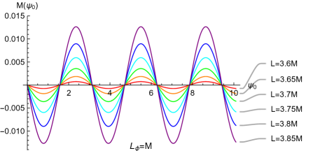
Figure 1: Dependence of the Melnikov function $\mathcal{M}\left(\psi_{0}\right)$ on the angular momentum $L$. We take $m=1$ and $L_{\phi}=M$. Left Panel: $\mathcal{M}\left(\psi_{0}\right)$ as a function of $\psi_{0}$ for various values of $L$. It shows that $\mathcal{M}\left(\psi_{0}\right)$ is a periodic function with the period of $\pi$, and $\mathcal{M}\left(\psi_{0}\right)$ has simple zeros at the points $\psi_{0}=n\pi/2$ with $n\in Z$. Right Panel: $\mathcal{M}\left(\psi_{0}=5\pi/4\right)$ as a function of $L/M$ on the interval of $2\sqrt{3}<L/M<4$. The amplitude of $\mathcal{M}\left(\psi_{0}\right)$ increases with increasing $L$.

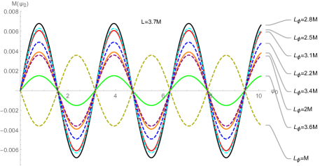
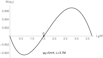
Figure 2: Dependence of the Melnikov function $\mathcal{M}\left(\psi_{0}\right)$ on the $z$-component of the angular momentum $L_{\phi}$. We take $m=1$ and $L=3.7M$. Left Panel: $\mathcal{M}\left(\psi_{0}\right)$ as a function of $\psi_{0}$ for various values of $L_{\phi}$. $\mathcal{M}\left(\psi_{0}\right)$ has simple zeros at the points $\psi_{0}=n\pi/2$ with $n\in Z$. Right Panel: $\mathcal{M}\left(\psi_{0}=5\pi/4\right)$ as a function of $L_{\phi}/M$ on the interval of $0\leq L_{\phi}\leq L$. $\mathcal{M}\left(\psi_{0}\right)=0$ when $L_{\phi}=0$, $L_{\phi}=L$ and at the point $C$, where $L_{\phi}/M\simeq 1.53$. The amplitude of $\mathcal{M}\left(\psi_{0}\right)$ has two local maximum values at $L_{\phi}/M\simeq 0.63$ and $2.80$, respectively.

The Melnikov function $\mathcal{M}\left(\psi_{0}\right)$ is quite complex and cannot be expressed in closed form. Nevertheless, $\mathcal{M}\left(\psi_{0}\right)$ can be computed numerically, and simple zeros of $\mathcal{M}\left(\psi_{0}\right)$ can be observed in its plot. Eqn. $\left(\ref{eq:M}\right)$ shows that, except the prefactor $\beta m^{5}M$, the behavior of $\mathcal{M}\left(\psi_{0}\right)$ only depends on two dimensionless parameters $L/M$ and $L_{\phi}/M$. So we depict how $\mathcal{M}\left(\psi_{0}\right)$ depends on $L/M$ and $L_{\phi}/M$ in FIGs. 1 and 2, respectively. The Melnikov function $\mathcal{M}\left(\psi_{0}\right)$ is plotted for various values of $L/M$ with fixed value of $L_{\phi}/M$ (i.e., $L_{\phi}/M=1$) in the left panel of FIG. 1, where we take $m=1$ without loss of generality. As expected, the periodic function $\mathcal{M}\left(\psi_{0}\right)$ has same period $\pi$ as the periodic coordinate $\psi$. More interestingly, $\mathcal{M}\left(\psi_{0}\right)$ is shown to have simple zeros at the points $\psi_{0}=n\pi/2$ with $n\in Z$, which means that the system exhibits chaotic feature. The panel also shows that the amplitude of $\mathcal{M}\left(\psi_{0}\right)$ monotonically grows as the value of $L/M$ increases. This behavior is also displayed in the right panel, in which the value of $\mathcal{M}\left(\psi_{0}\right)$ at $\psi_{0}=5\pi/4$ is plotted against $L/M$. In the left panel of FIG. 2, $\mathcal{M}\left(\psi_{0}\right)$ is plotted for various values of $L_{\phi}/M$ with fixed value of $L/M$ (i.e., $L/M=3.7$). It also shows that $\mathcal{M}\left(\psi_{0}\right)$ oscillates around zero with $\mathcal{M}\left(\psi_{0}\right)=0$ at $\psi_{0}=n\pi/2$ with $n\in Z$. The Melnikov function $\mathcal{M}\left(\psi_{0}\right)$ is shown to have the maximum amplitude at $L_{\phi}/M\simeq 2.8$. To better illustrate the dependence of the amplitude of $\mathcal{M}\left(\psi_{0}\right)$ on $L_{\phi}/M$, we plot $\mathcal{M}\left(\psi_{0}=5\pi/4\right)$ as a function of $L_{\phi}/M$ in the right panel of FIG. 2, in which two local maxima of the amplitude of $\mathcal{M}\left(\psi_{0}\right)$ at $L_{\phi}/M\simeq 0.63$ and $2.80$ can be seen. The amplitude of $\mathcal{M}\left(\psi_{0}\right)$ is zero for $L_{\phi}=0$ and $L_{\phi}=L$, which is expected since the integrand in eqn. $\left(\ref{eq:M0}\right)$ is periodic and independent of $\psi_{0}$ when $L_{\phi}=0$ and $L_{\phi}=L$ (can be seen from eqn. $\left(\ref{eq:H0H1}\right)$). Moreover, it displays that the amplitude of $\mathcal{M}\left(\psi_{0}\right)$ is also zero for $L_{\phi}/M\simeq 1.53$. So $\mathcal{M}\left(\psi_{0}\right)=0$ for $L_{\phi}=0$, $L_{\phi}/M=L/M=3.7$ and $L_{\phi}/M\simeq 1.53$, which means that the homoclinic orbit is preserved, and hence there is no occurrence of Smale horseshoes chaotic motion in these cases.

IV Conclusion

In this paper, we used the Melnikov method to investigate the chaotic behavior in geodesic motion on a Schwarzschild metric perturbed by the minimal length effects. The unperturbed system is well known to be integrable. For the near integrable perturbed system, the Melnikov method is very powerful to detect the presence of chaotic structure by tracing simple zeros of the Melnikov function $\mathcal{M}\left(\psi_{0}\right)$. After the perturbed Hamiltonian for a massive particle of angular momentum per unit mass $L$ and $z$-component of the orbital angular momentum per unit mass $L_{\phi}$ was obtained, the Melnikov function $\mathcal{M}\left(\psi_{0}\right)$ was numerically evaluated by using the higher-dimensional generalization of the Melnikov method. We make three observations regarding $\mathcal{M}\left(\psi_{0}\right)$:

• When $L_{\phi}=0$, $L$ and $L_{C}$ with $0<L_{C}<L$, $\mathcal{M}\left(\psi_{0}\right)=0$, which implies that no Smale horseshoes chaotic motion is present in the perturbed system.

• When the amplitude of $\mathcal{M}\left(\psi_{0}\right)$ is not zero, $\mathcal{M}\left(\psi_{0}\right)$ is a periodic function with the period of $\pi$, and has simple zeros at $\psi_{0}=n\pi/2$ with $n\in Z$, which signals the appearance of Smale horseshoes chaotic structure in the perturbed system.

• The amplitude of $\mathcal{M}\left(\psi_{0}\right)$ increases as $L$ increases with fixed $L_{\phi}$. When $L$ is fixed, the amplitude of $\mathcal{M}\left(\psi_{0}\right)$ as a function of $L_{\phi}$ has two local maxima.

The Melnikov’s method provides necessary but not sufficient condition for chaos and serves as an independent check on numerical tests for chaos. So it would be interesting to use other chaos indicators, e.g., the Poincare surfaces of section, the Lyapunov characteristic exponents and the method of fractal basin boundaries, to detect chaotic behavior in systems perturbed by the minimal length effects. In IN-Lu:2018mpr , we calculated the minimal length effects on the Lyapunov exponent of a massive particle perturbed away from an unstable equilibrium near the black hole horizon and found that the classical trajectory in black holes becomes more chaotic, which is consistent with the chaotic behavior found in this paper. Finally, the minimal length effects on the dual conformal field theory was analyzed in CON-Faizal:2017dlb . It is tempting to understand the holographic aspects of these chaotic behavior.

- (1) B. Carter, “Global structure of the Kerr family of gravitational fields,” Phys. Rev. 174, 1559 (1968). doi:10.1103/PhysRev.174.1559
- (2) Y. Sota, S. Suzuki and K. i. Maeda, “Chaos in static axisymmetric space-times. 1: Vacuum case,” Class. Quant. Grav. 13, 1241 (1996) doi:10.1088/0264-9381/13/5/034 [gr-qc/9505036].
- (3) W. Hanan and E. Radu, “Chaotic motion in multi-black hole spacetimes and holographic screens,” Mod. Phys. Lett. A 22, 399 (2007) doi:10.1142/S0217732307022815 [gr-qc/0610119].
- (4) J. R. Gair, C. Li and I. Mandel, “Observable Properties of Orbits in Exact Bumpy Spacetimes,” Phys. Rev. D 77, 024035 (2008) doi:10.1103/PhysRevD.77.024035 [arXiv:0708.0628 [gr-qc]].
- (5) V. Witzany, O. Semerák and P. Suková, “Free motion around black holes with discs or rings: between integrability and chaos – IV,” Mon. Not. Roy. Astron. Soc. 451, no. 2, 1770 (2015) doi:10.1093/mnras/stv1148 [arXiv:1503.09077 [astro-ph.HE]].
- (6) M. Wang, S. Chen and J. Jing, “Chaos in the motion of a test scalar particle coupling to the Einstein tensor in Schwarzschild–Melvin black hole spacetime,” Eur. Phys. J. C 77, no. 4, 208 (2017) doi:10.1140/epjc/s10052-017-4792-y [arXiv:1605.09506 [gr-qc]].
- (7) S. Chen, M. Wang and J. Jing, “Chaotic motion of particles in the accelerating and rotating black holes spacetime,” JHEP 1609, 082 (2016) doi:10.1007/JHEP09(2016)082 [arXiv:1604.02785 [gr-qc]].
- (8) C. Y. Liu, “Chaotic Motion of Charged Particles around a Weakly Magnetized Kerr-Newman Black Hole,” arXiv:1806.09993 [gr-qc].
- (9) A. V. Frolov and A. L. Larsen, “Chaotic scattering and capture of strings by black hole,” Class. Quant. Grav. 16, 3717 (1999) doi:10.1088/0264-9381/16/11/316 [gr-qc/9908039].
- (10) L. A. Pando Zayas and C. A. Terrero-Escalante, “Chaos in the Gauge / Gravity Correspondence,” JHEP 1009, 094 (2010) doi:10.1007/JHEP09(2010)094 [arXiv:1007.0277 [hep-th]].
- (11) D. Z. Ma, J. P. Wu and J. Zhang, “Chaos from the ring string in a Gauss-Bonnet black hole in AdS5 space,” Phys. Rev. D 89, no. 8, 086011 (2014) doi:10.1103/PhysRevD.89.086011 [arXiv:1405.3563 [hep-th]].
- (12) D. Z. Ma, D. Zhang, G. Fu and J. P. Wu, “Chaotic dynamics of string around charged black brane with hyperscaling violation,” JHEP 2001, 103 (2020) doi:10.1007/JHEP01(2020)103 [arXiv:1911.09913 [hep-th]].
- (13) V. K. Mel’nikov, “On the stability of a center for time-periodic perturbations”, Tr. Mosk. Mat. Obs., 12, 1963, 3–52
- (14) L. Bombelli and E. Calzetta, “Chaos around a black hole,” Class. Quant. Grav. 9, 2573 (1992). doi:10.1088/0264-9381/9/12/004
- (15) P. S. Letelier and W. M. Vieira, “Chaos in black holes surrounded by gravitational waves,” Class. Quant. Grav. 14, 1249 (1997) doi:10.1088/0264-9381/14/5/026 [gr-qc/9706025].
- (16) M. Santoprete and G. Cicogna, “Chaos in black holes surrounded by electromagnetic fields,” Gen. Rel. Grav. 34, 1107 (2002) doi:10.1023/A:1016570106387 [nlin/0110046 [nlin-cd]].
- (17) L. Polcar and O. Semerák, “Free motion around black holes with discs or rings: Between integrability and chaos. VI. The Melnikov method,” Phys. Rev. D 100, no. 10, 103013 (2019) doi:10.1103/PhysRevD.100.103013 [arXiv:1911.09790 [gr-qc]].
- (18) M. Chabab, H. El Moumni, S. Iraoui, K. Masmar and S. Zhizeh, “Chaos in charged AdS black hole extended phase space,” Phys. Lett. B 781, 316 (2018) doi:10.1016/j.physletb.2018.04.014 [arXiv:1804.03960 [hep-th]].
- (19) S. Mahish and B. Chandrasekhar, “Chaos in Charged Gauss-Bonnet AdS Black Holes in Extended Phase Space,” Phys. Rev. D 99, no. 10, 106012 (2019) doi:10.1103/PhysRevD.99.106012 [arXiv:1902.08932 [hep-th]].
- (20) Y. Chen, H. Li and S. J. Zhang, “Chaos in Born–Infeld–AdS black hole within extended phase space,” Gen. Rel. Grav. 51, no. 10, 134 (2019) doi:10.1007/s10714-019-2612-4 [arXiv:1907.08734 [hep-th]].
- (21) C. Dai, S. Chen and J. Jing, “Thermal chaos of a charged dilaton-AdS black hole in the extended phase space,” arXiv:2002.01641 [gr-qc].
- (22) G. Veneziano, “A Stringy Nature Needs Just Two Constants,” Europhys. Lett. 2, 199 (1986). doi:10.1209/0295-5075/2/3/006
- (23) D. J. Gross and P. F. Mende, “String Theory Beyond the Planck Scale,” Nucl. Phys. B 303, 407 (1988). doi:10.1016/0550-3213(88)90390-2
- (24) D. Amati, M. Ciafaloni and G. Veneziano, “Can Space-Time Be Probed Below the String Size?,” Phys. Lett. B 216, 41 (1989). doi:10.1016/0370-2693(89)91366-X
- (25) L. J. Garay, “Quantum gravity and minimum length,” Int. J. Mod. Phys. A 10, 145 (1995) doi:10.1142/S0217751X95000085 [gr-qc/9403008].
- (26) M. Maggiore, “The Algebraic structure of the generalized uncertainty principle,” Phys. Lett. B 319, 83 (1993) doi:10.1016/0370-2693(93)90785-G [hep-th/9309034].
- (27) A. Kempf, G. Mangano and R. B. Mann, “Hilbert space representation of the minimal length uncertainty relation,” Phys. Rev. D 52, 1108 (1995) doi:10.1103/PhysRevD.52.1108 [hep-th/9412167].
- (28) L. N. Chang, D. Minic, N. Okamura and T. Takeuchi, “Exact solution of the harmonic oscillator in arbitrary dimensions with minimal length uncertainty relations,” Phys. Rev. D 65, 125027 (2002) doi:10.1103/PhysRevD.65.125027 [hep-th/0111181].
- (29) R. Akhoury and Y. P. Yao, “Minimal length uncertainty relation and the hydrogen spectrum,” Phys. Lett. B 572, 37 (2003) doi:10.1016/j.physletb.2003.07.084 [hep-ph/0302108].
- (30) F. Brau, “Minimal length uncertainty relation and hydrogen atom,” J. Phys. A 32, 7691 (1999) doi10.1088/0305-4470/32/44/308 [quant-ph/9905033].
- (31) F. Brau and F. Buisseret, “Minimal Length Uncertainty Relation and gravitational quantum well,” Phys. Rev. D 74, 036002 (2006) doi:10.1103/PhysRevD.74.036002 [hep-th/0605183].
- (32) P. Pedram, K. Nozari and S. H. Taheri, “The effects of minimal length and maximal momentum on the transition rate of ultra cold neutrons in gravitational field,” JHEP 1103, 093 (2011) doi:10.1007/JHEP03(2011)093 [arXiv:1103.1015 [hep-th]].
- (33) I. Pikovski, M. R. Vanner, M. Aspelmeyer, M. S. Kim and C. Brukner, “Probing Planck-scale physics with quantum optics,” Nature Phys. 8, 393 (2012) doi:10.1038/nphys2262 [arXiv:1111.1979 [quant-ph]].
- (34) P. Bosso, S. Das and R. B. Mann, “Potential tests of the Generalized Uncertainty Principle in the advanced LIGO experiment,” Phys. Lett. B 785, 498 (2018) doi:10.1016/j.physletb.2018.08.061 [arXiv:1804.03620 [gr-qc]].
- (35) P. Wang, H. Yang and X. Zhang, “Quantum gravity effects on statistics and compact star configurations,” JHEP 1008, 043 (2010) doi:10.1007/JHEP08(2010)043 [arXiv:1006.5362 [hep-th]].
- (36) Y. C. Ong, “Generalized Uncertainty Principle, Black Holes, and White Dwarfs: A Tale of Two Infinities,” JCAP 1809, no. 09, 015 (2018) doi:10.1088/1475-7516/2018/09/015 [arXiv:1804.05176 [gr-qc]].
- (37) S. Benczik, L. N. Chang, D. Minic, N. Okamura, S. Rayyan and T. Takeuchi, “Short distance versus long distance physicsThe Classical limit of the minimal length uncertainty relation,” Phys. Rev. D 66, 026003 (2002) doi10.1103/PhysRevD.66.026003 [hep-th/0204049].
- (38) Z. K. Silagadze, “Quantum gravity, minimum length and Keplerian orbits,” Phys. Lett. A 373, 2643 (2009) doi:10.1016/j.physleta.2009.05.053 [arXiv:0901.1258 [gr-qc]].
- (39) F. Ahmadi and J. Khodagholizadeh, “Effect of GUP on the Kepler problem and a variable minimal length,” Can. J. Phys. 92, 484 (2014) doi:10.1139/cjp-2013-0354 [arXiv:1411.0241 [hep-th]].
- (40) F. Scardigli and R. Casadio, “Gravitational tests of the Generalized Uncertainty Principle,” Eur. Phys. J. C 75, no. 9, 425 (2015) doi:10.1140/epjc/s10052-015-3635-y [arXiv:1407.0113 [hep-th]].
- (41) A. Farag Ali, M. M. Khalil and E. C. Vagenas, “Minimal Length in quantum gravity and gravitational measurements,” Europhys. Lett. 112, no. 2, 20005 (2015) doi:10.1209/0295-5075/112/20005 [arXiv:1510.06365 [gr-qc]].
- (42) X. Guo, P. Wang and H. Yang, “The classical limit of minimal length uncertainty relation: revisit with the Hamilton-Jacobi method,” JCAP 1605, no. 05, 062 (2016) doi:10.1088/1475-7516/2016/05/062 [arXiv:1512.03560 [gr-qc]].
- (43) M. Khodadi, K. Nozari and A. Hajizadeh, “Some Astrophysical Aspects of a Schwarzschild Geometry Equipped with a Minimal Measurable Length,” Phys. Lett. B 770, 556 (2017) doi:10.1016/j.physletb.2017.05.016 [arXiv:1702.06357 [gr-qc]].
- (44) F. Scardigli and R. Casadio, “Perihelion Precession and Generalized Uncertainty Principle,” Springer Proc. Phys. 208, 149 (2018).
- (45) J. Tao, P. Wang and H. Yang, “Homogeneous Field and WKB Approximation In Deformed Quantum Mechanics with Minimal Length,” Adv. High Energy Phys. 2015, 718359 (2015) doi:10.1155/2015/718359 [arXiv:1211.5650 [hep-th]].
- (46) T. S. Quintela, Jr., J. C. Fabris and J. A. Nogueira, “The Harmonic Oscillator in the Classical Limit of a Minimal-Length Scenario,” Braz. J. Phys. 46, no. 6, 777 (2016) doi:10.1007/s13538-016-0457-9 [arXiv:1510.08129 [hep-th]].
- (47) V. M. Tkachuk, “Deformed Heisenberg algebra with minimal length and equivalence principle,” Phys. Rev. A 86, 062112 (2012) doi:10.1103/PhysRevA.86.062112 [arXiv:1301.1891 [gr-qc]].
- (48) F. Scardigli, G. Lambiase and E. Vagenas, “GUP parameter from quantum corrections to the Newtonian potential,” Phys. Lett. B 767, 242 (2017) doi:10.1016/j.physletb.2017.01.054 [arXiv:1611.01469 [hep-th]].
- (49) Q. Zhao, M. Faizal and Z. Zaz, “Short distance modification of the quantum virial theorem,” Phys. Lett. B 770, 564 (2017) doi:10.1016/j.physletb.2017.01.029 [arXiv:1707.00636 [hep-th]].
- (50) B. Mu and J. Tao, “Minimal Length Effect on Thermodynamics and Weak Cosmic Censorship Conjecture in anti-de Sitter Black Holes via Charged Particle Absorption,” arXiv:1906.10544 [gr-qc].
- (51) F. Lu, J. Tao and P. Wang, “Minimal Length Effects on Chaotic Motion of Particles around Black Hole Horizon,” JCAP 1812, 036 (2018) doi:10.1088/1475-7516/2018/12/036 [arXiv:1811.02140 [gr-qc]].
- (52) H. Hassanabadi, E. Maghsoodi and W. Sang Chung, “Analysis of motion of particles near black hole horizon under generalized uncertainty principle,” EPL 127, no. 4, 40002 (2019). doi:10.1209/0295-5075/127/40002
- (53) D. Chen, H. Wu and H. Yang, “Observing remnants by fermions’ tunneling,” JCAP 1403, 036 (2014) doi:10.1088/1475-7516/2014/03/036 [arXiv:1307.0172 [gr-qc]].
- (54) D. Y. Chen, Q. Q. Jiang, P. Wang and H. Yang, “Remnants, fermions‘ tunnelling and effects of quantum gravity,” JHEP 1311, 176 (2013) doi:10.1007/JHEP11(2013)176 [arXiv:1312.3781 [hep-th]].
- (55) D. Chen, H. Wu, H. Yang and S. Yang, “Effects of quantum gravity on black holes,” Int. J. Mod. Phys. A 29, no. 26, 1430054 (2014) doi:10.1142/S0217751X14300543 [arXiv:1410.5071 [gr-qc]].
- (56) E. Maghsoodi, H. Hassanabadi and W. Sang Chung, “Black hole thermodynamics under the generalized uncertainty principle and doubly special relativity,” PTEP 2019, no. 8, 083E03 (2019) doi:10.1093/ptep/ptz085 [arXiv:1901.10305 [physics.gen-ph]].
- (57) S. Wiggins, “Introduction to Applied Nonlinear Dynamical Systems and Chaos (Second Ed.),” Springer-Verlag, New York and Bristol, 2003.
- (58) P. J. Holmes and J. E. Marsden, “Horseshoes and Arnold diffusion for Hamiltonian Systems on Lie groups,” Indiana Univ. Math. J. 32, 273 (1983).
- (59) B. Mu, P. Wang and H. Yang, “Minimal Length Effects on Tunnelling from Spherically Symmetric Black Holes,” Adv. High Energy Phys. 2015, 898916 (2015) doi:10.1155/2015/898916 [arXiv:1501.06025 [gr-qc]].
- (60) M. Faizal, A. F. Ali and A. Nassar, “Generalized uncertainty principle as a consequence of the effective field theory,” Phys. Lett. B 765, 238 (2017) doi:10.1016/j.physletb.2016.11.054 [arXiv:1701.00341 [hep-th]].