Evidence for Spin-orbit Alignment in the TRAPPIST-1 System

Abstract

In an effort to measure the Rossiter-McLaughlin effect for the TRAPPIST-1 system, we performed high-resolution spectroscopy during transits of planets e, f, and b. The spectra were obtained with the InfraRed Doppler spectrograph on the Subaru 8.2-m telescope, and were supplemented with simultaneous photometry obtained with a 1-m telescope of the Las Cumbres Observatory Global Telescope. By analyzing the anomalous radial velocities, we found the projected stellar obliquity to be $\lambda=1\pm 28$ degrees under the assumption that the three planets have coplanar orbits, although we caution that the radial-velocity data show correlated noise of unknown origin. We also sought evidence for the expected deformations of the stellar absorption lines, and thereby detected the “Doppler shadow” of planet b with a false alarm probability of $1.7\,\%$. The joint analysis of the observed residual cross-correlation map including the three transits gave $\lambda=19_{-15}^{+13}$ degrees. These results indicate that the the TRAPPIST-1 star is not strongly misaligned with the common orbital plane of the planets, although further observations are encouraged to verify this conclusion.

1 Introduction

Measuring the stellar obliquity (the angle between a star’s spin axis and the orbital axis of a planet) is an important method to probe the dynamical history of exoplanets. Unlike the Solar System, in which the planets’ orbital planes are aligned with the solar equator to within about $6^{\circ}$, measurements of the Rossiter-McLaughlin (RM) effect (Rossiter, 1924; McLaughlin, 1924) have revealed that stars with short-period giant planets have a broad range of obliquities (Triaud et al., 2010; Albrecht et al., 2012). This finding has led to many proposals for mechanisms that could have tilted the orbital or the spin axes (see, e.g., Fabrycky & Tremaine, 2007; Nagasawa et al., 2008; Bate et al., 2010; Rogers et al., 2012; Batygin & Adams, 2013).

The obliquities of stars with multiple transiting planets in coplanar orbits — particularly those lacking massive companions on wide orbits — are interesting and relatively unexplored. Such systems may provide the opportunity to probe the “primordial” obliquities of planet-hosting stars. The orbital coplanarity suggests that these systems have not experienced major dynamical rearrangements due to planet-planet scattering (Fang & Margot, 2012), and the lack of a massive companion on a wide orbit removes the possibility that the planetary orbital plane has been tilted by secular gravitational perturbations. The stellar obliquity has only been measured for a small number of multiple-planet systems. In most cases, the obliquity is small (e.g., Sanchis-Ojeda et al., 2012; Hirano et al., 2012; Albrecht et al., 2013), although there are at least two systems with large misalignments (Huber et al., 2013; Dalal et al., 2019).

TRAPPIST-1 is a cool M dwarf ($T_{\rm eff}\approx 2{,}550$ K) known to host seven transiting planets (Gillon et al., 2016, 2017). The system has attracted particular attention because the third, fourth, and fifth planets (e, f, and g) reside inside or near the “habitable zone” of the host star. The orbital periods of the planets are also close to mean-motion resonances, leading to detectable transit-timing variations (TTVs) that have been used to constrain the masses of all seven planets. The latest such analysis found that the planets have a mainly rocky composition (Grimm et al., 2018). The existence of resonances and the coplanarity of the orbits both suggest that the planets were drawn together by convergent migration within the protoplanetary disk (i.e., type I migration; Lubow & Ida, 2010). Moreover, no stellar companion has been detected which could have disturbed the initial alignment between the stellar equator and the protoplanetary disk (Howell et al., 2016).

During a 6-hour interval on the night of UT 2018 August 31, three of the planets in the TRAPPIST-1 system (planets e, f, and b) sequentially transited the star. We took advantage of this opportunity to try and measure the stellar obliquity, by performing high-resolution infrared spectroscopy with the InfraRed Doppler (IRD) instrument mounted on the Subaru 8.2-m telescope on Maunakea (Kotani et al., 2018). This new instrument has a resolution of approximately 70,000 and a spectral range of 0.95 to 1.75 $\mu$m; TRAPPIST-1 is extremely faint in the visible, and these kinds of characterizations are only feasible in the near infrared.

2 Observations

2.1 High Dispersion Spectroscopy with Subaru/IRD

We observed TRAPPIST-1 with the IRD spectrograph for 7 hours spanning almost all of the transit of planet e, followed by the complete transits of planets f and b. The exposure time was 300 seconds. Beforehand, we observed a rapidly rotating A0 star (HD 195689; Cannon & Pickering, 1993) to help with telluric corrections. For simultaneous wavelength calibration, the light from a laser-frequency comb (LFC) was injected into the spectrograph using a second fiber. To support our analysis, we also used a few IRD spectra of TRAPPIST-1 that were obtained when no planets were transiting, in 2018 December, 2019 January, and 2019 July. These spectra were used to construct a telluric-free stellar template for the RV analysis, exploiting the variation in the stellar RV due to Earth’s orbital motion.

We reduced the raw IRD data with the echelle package of IRAF, for the most part. We extracted wavelength-calibrated one-dimensional (1-d) spectra for each stellar spectrum and the accompanying LFC spectrum. On the transit night, the signal-to-noise ratio (S/N) of the 1-d stellar spectrum varied within the range of 15 to 25 per pixel at $1\,\mu$m, and 45 to 50 per pixel at $1.6\,\mu$m.

2.2 Simultaneous Photometry

We also performed time-series photometry of TRAPPIST-1 on the transit night, using one of the McDonald 1-m telescopes of the Las Cumbres Observatory Global Telescope (LCOGT) network. The main purpose was to provide stronger constraints on the mid-transit times. We observed with the SINISTRO CCD camera and a Cousins $I$-band filter for 4.8 hours spanning the transits of planets e and f. Given the apparent magnitude of TRAPPIST-1 ($m_{I}=14$) we used 60-second exposures.

The images were reduced by the BANZAI pipeline (McCully et al., 2018), and aperture photometry was performed with a custom code (Fukui et al., 2011). Photometry was also performed on five nearby and isolated stars, to allow for correction of the effects due to differential extinction by the Earth’s atmosphere. The comparison stars were brighter than TRAPPIST-1 in the $I$-band by 1.1 to 1.5 magnitudes. After trying various sizes for the photometric aperture, we settled on a radius of 8 pixels, which was found to minimize the scatter in the differential light curve. The bottom panel of Figure 1 shows the light curve.

3 Data Analysis

3.1 Radial Velocities

We extracted RVs from the IRD spectra using the following procedure. The total spectral range was divided into $\approx 1200$ spectral segments, each spanning a wavelength range of $\Delta\lambda=0.7-1.0$ nm. The LFC spectra were used to model the instantaneous instrumental profile (IP) of each spectral segment. Using this IP model, we extracted a template spectrum by deconvolving each TRAPPIST-1 spectrum and removing telluric absorption features. The telluric lines are identified and removed using normalized spectra of the rapidly-rotating A0 star for most cases, but we also removed those lines by fitting a theoretical transmittance (Clough et al., 2005) in case that no telluric standard star is observed immediately before or after our observation of TRAPPIST-1 (UT 2018 August 7 and December 25). We shifted the resulting spectra with wavelength into a common frame of reference by cross-correlating telluric-free spectral segments against a theoretical model spectrum for TRAPPIST-1 (Allard et al., 2013). Then, we median-combined the spectra to obtain a deconvolved and telluric-corrected template spectrum, representing our best estimate of the intrinsic spectrum of TRAPPIST-1.

Using this template spectrum $S(\lambda)$, we modeled each IRD spectral segment $f_{\mathrm{obs}}(\lambda)$ as

$$f_{\mathrm{obs}}(\lambda)=k(\lambda)\times\left[S\left(\lambda\sqrt{\frac{1+v/c}{1-v/c}}\right)\times T(\lambda)\right]\otimes\mathrm{IP},$$ (1)

where $v$ is the RV, $\otimes$ is the convolution operator, $k(\lambda)$ is a quadratic function of vacuum wavelength $\lambda$ that was included to account for the overall continuum variation, $T(\lambda)$ is a model of telluric transmittance (Clough et al., 2005), and IP is the estimated instrumental profile. After optimizing the model by Markov Chain Monte Carlo (MCMC) samplings using our customized code for each segment, we determined the RV value and its uncertainty based on the weighted mean of $v$ across all the spectral segments that did not show especially strong telluric absorption features. The RVs on the transit night are shown by the blue points in the top panel of Figure 1.

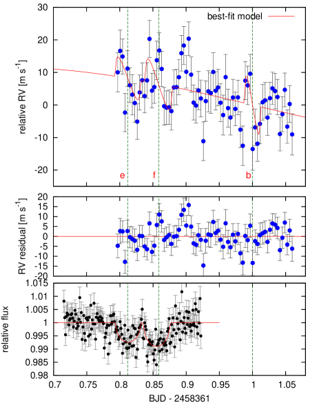
Figure 1: Top: Relative RVs measured with Subaru/IRD (blue points) and the best-fitting model (red line). Note that the RV value at $T_{c}$ of planet b is set to zero (the systemic velocity of TRAPPIST-1 ($\approx-52.5$ km s^-1) was subtracted). Middle: Residuals. Bottom: Simultaneous photometry from LCOGT/SINISTRO (black points) and the best-fitting model (red line). The vertical dashed lines are the best estimates of the transit midpoints.

3.2 Refining Transit Ephemerides

To pin down the mid-transit times, we jointly analyzed the LCOGT data and the available Kepler data. The Kepler telescope observed TRAPPIST-1 in short-cadence mode (one-minute integrations) during Campaign 19 of the K2 mission. We downloaded the pixel-level data from the Mikulski Archive for Space Telescopes (MAST). The data from the first 8.5 days of the campaign were unusable because of an error in spacecraft pointing. The K2 data span ten transits of planet b, and three transits each of planets e and f. We performed aperture photometry and reduced the systematic effects from the telescope’s rolling motion following a standard procedure described by Dai et al. (2017). We found that a circular aperture with a radius of 2.5 pixels minimized the out-of-transit scatter in the light curve.

Table 1: Transit Ephemerides. These results were used to set Gaussian priors for $T_{c}$ in the RM analyses.

Planet	$P$ (days)	$T_{c}$ ($\mathrm{BJD}_{\mathrm{TDB}}$)
b	$1.51087_{-0.00017}^{+0.00022}$	$2458362.0021_{-0.0022}^{+0.0016}$
e	$6.09705_{-0.00093}^{+0.00096}$	$2458361.8113_{-0.0025}^{+0.0028}$
f	$9.2129\pm 0.0010$	$2458361.8545\pm 0.0018$

Although the TRAPPIST-1 planets are known to experience TTVs (Gillon et al., 2016), we assumed the periods to be constant while fitting the LCOGT and K2 data. This is because the LCOGT and K2 observations were only separated by about seven days, and the TTVs on such short timescales are negligible (Grimm et al., 2018). We performed the transit modeling with the Batman package (Kreidberg, 2015), adopting a quadratic limb-darkening law with freely adjustable coefficients for each of the two bandpasses. The other transit parameters (radius ratio $R_{p}/R_{s}$, impact parameter $b$, period $P$, and reference mid-transit time $T_{c}$) were assumed to be the same across both data sets. We assumed the orbits to be circular, and imposed a Gaussian prior on the mean stellar density of $50.7^{+1.2}_{-2.2}\,\rho_{\odot}$ (Gillon et al., 2016), which acts effectively as a constraint on the scaled semi-major axis $a/R_{s}$. We performed an MCMC analysis with the emcee package (Foreman-Mackey et al., 2013). Table 1 gives the results for the orbital periods and transit midpoints.

3.3 Modeling of the RM Effect

The RVs on the transit night (Figure 1) show some of the patterns that are expected from the RM effect, along with some other variations that are not associated with the transits. Because of the low S/N ratio and lack of RV points before the transits of planet e and f, we decided to assume that the projected obliquity $\lambda$ is the same for all three planets, instead of trying to determine the projected obliquity relative to each of the planetary orbits. To model the anomalous RV due to the RM effect, we used the formulas presented by Hirano et al. (2011). The free parameters were $\lambda$, the projected rotation velocity $v\sin i_{s}$, and the slope and intercept of a linear function of time. The intercept represents the arbitrary RV offset $\gamma$, and the slope represents the apparent acceleration of star throughout the transit night. This is partly from the gravitational acceleration from the combined pull of all the planets, but may also include systematic effects from stellar activity, telluric effects, or instrumental variations. To avoid having to mitigate the effects of long-term stellar activity and account for the orbital motion of all seven planets, we only fitted the data from the transit night. The transit midpoints were allowed to vary subject to Gaussian priors based on the values in Table 1. The transit impact parameter $b$ is known to correlate with $v\sin i_{s}$ and $\lambda$, especially when $b$ is close to zero (e.g., Albrecht et al., 2011), and hence we also let $b$ float with Gaussian priors based on the literature values (Gillon et al., 2017). The other transit parameters were held fixed at the values reported in the literature (Gillon et al., 2017).

We performed an MCMC analysis using the code described by Hirano et al. (2016). The best-fitting model has $\chi^{2}=81.4$ with 68 degrees of freedom. Table 2 gives the results for the parameters, which are based on the 16%, 50%, and 84% levels of the marginalized cumulative posterior distributions. The red curve in the top panel of Figure 1 shows the best-fitting model, and the middle panel shows the residuals when the model RVs are subtracted from the observed RVs.

Table 2: Estimated RM Parameters and Their Priors. The symbol $\mathcal{U}$ represents a uniform prior.

Planet	b	e	f	Imposed Prior
Effective RV analysis
$v\sin i_{s}$ (km s-1) (three transits combined)		$1.50\pm 0.37$		$\mathcal{U}\,[-\infty,+\infty]$
$\lambda$ (deg.) (three transits combined)		$1\pm 28$		$\mathcal{U}\,[-180,+180]$
Doppler shadow
$v\sin i_{s}$ (km s-1)	$2.16_{-0.55}^{+0.17}$	$1.74_{-0.75}^{+0.43}$	$1.85_{-0.73}^{+0.20}$	$\mathcal{U}\,[0.6,2.4]$
$\lambda$ (deg.)	$15_{-30}^{+26}$	$9_{-51}^{+45}$	$21\pm 32$	$\mathcal{U}\,[-180,+180]$
$v\sin i_{s}$ (km s-1) (three transits combined)		$2.04_{-0.16}^{+0.18}$		$\mathcal{U}\,[0.6,2.4]$
$\lambda$ (deg.) (three transits combined)		$19_{-15}^{+13}$		$\mathcal{U}\,[-180,+180]$

The result for the projected obliquity is $\lambda=1\pm 28$ degrees, consistent with spin-orbit alignment of the TRAPPIST-1 system. The result for the projected rotation velocity is $v\sin i_{s}=1.49_{-0.37}^{+0.36}$ km s^-1. As a consistency check, it is useful to compare this result for $v\sin i_{s}$ with the value of the rotation velocity, $v=2\pi R_{s}/P_{\rm rot}$, based on the stellar radius $R_{s}$ and rotation period $P$. To estimate $P_{\rm rot}$, we inspected the K2 light curve for signs of periodic photometric variability. The Lomb-Scargle periodogram (Lomb, 1976; Scargle, 1982) shows a peak at 3.28 days, and the auto-correlation function leads to a period of 3.25 days. Both of these estimates are in agreement with the period reported by Luger et al. (2017). In combination with $R_{s}=0.117\,R_{\odot}$ (Gillon et al., 2016), the calculated rotation velocity is 1.8 km s^-1. This is consistent with our result for $v\sin i_{s}$, and therefore consistent with a low stellar obliquity. We note, though, that our result for $v\sin i_{s}$ is lower than the value of $6\pm 2$ km s^-1 reported by Reiners & Basri (2010), which we believe was mistaken. In fact, the high value of $v\sin i_{s}$ reported earlier made the prospect of RM observations appear easier than it was in reality; for instance, Cloutier & Triaud (2016) predicted an RM amplitude of $40-50$ m s^-1 based on this larger $v\sin i_{s}$. To make sure that our measurement of $\lambda$ is not vulnerable to $v\sin i_{s}$, we fitted the RV data with $v\sin i_{s}$ being fixed at $1.8$ km s^-1. The result for $\lambda$ was unchanged, as expected ($\lambda=4_{-32}^{+30}$ degrees).

The residuals exhibit correlated patterns, particularly between $0.85$ and $0.90$ on the time axis of Figure 1. We do not know the origin of those features, and can only speculate that they are from stellar activity, flares, or instrumental effects. In order to quantify the impact of this correlated noise on $\lambda$, we performed a numerical experiment using the “prayer bead” method (e.g., Désert et al., 2009) as follows; Assuming that the residual data between the observed RVs and the best-fit model (middle panel of Figure 1) reflect the magnitude and timescale for the correlated noise, we created a series of mock RV data sets by adding cyclically permuted residual RVs (time stamps shifted one by one) to the best-fit model in Figure 1, thus generating $72$ sets of mock RV data. We then fitted each mock data set using the same code as above. As a result of this numerical experiment, we found that the scatter in the best-fit $v\sin i_{s}$ and $\lambda$ were $0.51$ km s^-1 and $31$ degrees, respectively. These estimates of systematic errors are comparable to the statistical errors reported in Table 2.

4 The Doppler shadow

Given the large statistical and systematic uncertainties in $v\sin i_{s}$ and $\lambda$, it is reasonable to question the result for our fit to IRD RV data. We were thereby motivated to perform a second analysis of the RM effect, based on modeling the distortions in the line profiles rather than extracting an effective RV (see, e.g., Albrecht et al., 2007; Hirano et al., 2010; Collier Cameron et al., 2010). This technique is often called “Doppler tomography,” although we prefer to refer to the “Doppler transit” or “Doppler shadow” of the planet, because there is not much resemblance to the standard meaning of tomography.

In previous analyses of Doppler transits, the spectral line profiles have been modeled with least-squares deconvolution (LSD; Donati et al., 1997). In this case, though, most of the spectral information is from complex and blended molecular absorption lines, making it almost impossible to define the spectral continuum or analyze individual lines. Instead, we used the classical cross-correlation function (CCF) technique to extract the mean line profile. To generate a cross-correlation template, we deconvolved the individual IRD spectra using the instantaneous IP and a theoretical rotation/macroturbulence broadening kernel (Gray, 2005). We employed the iterative/recursive deconvolution technique described by Coggins et al. (1994) to extract the mean deconvolved spectrum of TRAPPIST-1, using a large number of out-of-transit spectra taken on multiple nights. For the deconvolution, we assumed $v\sin i_{s}=1.8$ km s^-1 based on the rotation period measurements described in Section 3.3, and the macroturbulent velocity of $\zeta=1$ km s^-1, following Valenti et al. (1998) and Bean et al. (2006). The resulting deconvolved, normalized spectrum, denoted by $S_{\mathrm{intrinsic}}$, represents our best estimate of TRAPPIST-1’s spectrum in the absence of rotation. This is needed to represent the emergent spectrum from the portion of the star that is blocked by a transiting planet.

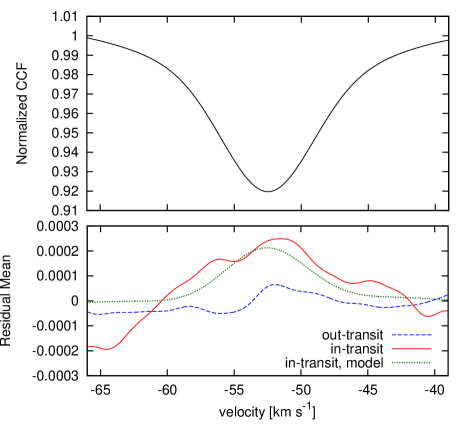
Figure 2: Top: Barycentric velocity (RV) vs. mean out-of-transit CCF between observed TRAPPIST-1’s spectra and its flipped template (i.e., $1-S_{\mathrm{intrinsic}}$). Note that the CCF has a minimum because the features being correlated are absorption lines. Bottom: Mean residual CCF during the transit of TRAPPIST-1b, stacked at the instantaneous planet shadow position in the profile (red solid line). Mean out-of-transit residual CCF, covering the same time interval, is shown by the blue dashed line. The green dotted line plots the theoretical mean in-transit residual CCF model. See Section 5 for more details.

For the CCF analysis, we divided the individual IRD spectra by the normalized A0 star spectrum to remove the telluric lines, taking into account the differences in airmass between the observation of the standard star and those of TRAPPIST-1 with a plane parallel atmosphere (e.g., Kawauchi et al., 2018). Then, we cross-correlated each processed IRD spectrum with $1-S_{\mathrm{intrinsic}}$, and normalized the resulting CCF. Finally, we corrected for the barycentric motion of the Earth for each CCF and translated the CCFs to a common velocity scale. The top panel of Figure 2 shows the mean CCF when no transits were occurring.

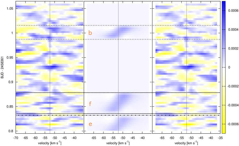
Figure 3: Left: Observed residual CCF map (velocity-time space) based on the IRD spectra for TRAPPIST-1. Middle: Best-fit theoretical model for the residual CCF map after the MCMC analysis. The observed CCF map exhibits some instantaneous variations on a timescale of 10–20 minutes. The impact of the correlated noise in discussed in Section 5. Right: Observed residual CCF map after subtracting the best-fit model.

To visualize the mean line-profile variations, we subtracted the mean out-of-transit CCF from each individual CCF, and examined the resulting residuals as a function of time. The raw residual CCF map exhibited an overall low-frequency modulation which is most likely due to a combination of detector persistence, variations in the signal-to-noise ratio, and the imperfect removal of telluric lines. To account for this slow modulation, we fitted a fourth-order polynomial function of time to the residual CCF and subtracted the polynomial from each velocity column. Since the timescale of CCF variations due to a transit (30–60 minutes) is much smaller than the observing span (7 hours) on that night, this step would not significantly diminish the planetary signal. The left panel of Figure 3 shows the resulting time series of residual CCFs, which were searched for the Doppler shadow of each planet.

The transit ingress and egress times are indicated by pairs of horizontal lines (for planet e, f, and b, from bottom to top). Given the star’s rotation velocity of about 2 km s^-1, any features on the photosphere should be shifted by no more than $2$ km s^-1 from the barycentric RV of $-52.5$ km s^-1. If the stellar obliquity is small, the planetary shadow appears as a loss of light that moves from the blue (left) side to the red (right) side of the line profile. In the figure, this would correspond to a blue bump that progresses from the lower left to the upper right of the rectangle spanned by the transit. Such a traveling bump does appear to be barely discernible for TRAPPIST-1b, but is not evident for the other planets.

For quantitative analysis, we created about 2,000 mock spectra mimicking the IRD data during a transit of each planet, following Hirano et al. (2011). To create each mock spectrum, we began with $S_{\mathrm{intrinsic}}$, and applied the same blaze function, IP, etc., as the real data. This was done for a range of possible values of $v\sin i_{s}$ from 0.6 to 2.4 km s^-1, and for the full range of positions of the planet on the stellar disk. We subjected the mock transit spectra to the same CCF analysis as the real data. The grid of values was fine enough to allow the residual CCF to be computed reliably for any values of $v\sin i_{s}$ and planet position, using linear interpolation.

This provided all the necessary ingredients for a model of the residual CCFs. We fitted the model to the real data for each of the three transits (i.e., for each planet). We performed an MCMC analysis to determine the parameters. We adopted uniform priors on $v\sin i_{s}$ and $\lambda$ and imposed the same Gaussian priors on the midtransit times and impact parameters $b$ that were described earlier. The only freely adjustable parameters were $v\sin i_{s}$ and $\lambda$ for each transit; the other transit parameters were held fixed at the values reported by Gillon et al. (2017). Table 2 gives the results. The best-fit obliquity $\lambda$ has large uncertainties for individual transits, but all the fitting results prefer a low obliquity (prograde orbit). Motivated by this fact, we performed a joint analysis assuming the same values of $v\sin i_{s}$ and $\lambda$ for all the three transits, and fitted the whole residual CCF data on the night. The projected obliquity was found to be $\lambda=19_{-15}^{+13}$ degrees, consistent with the result for the RV fit. The best-fit model of the residual CCF time series and the observed CCF map with the best-fit model subtracted are depicted in the middle and right panels of Figure 3, respectively.

5 Discussion and Summary

Besides $\lambda$, another parameter that deserves discussion is the overall slope of the RV time series on the transit night. If this apparent acceleration were entirely due the gravitational forces from the planets, the dominant effect would be from planet b. Under this interpretation, the best-fitting slope corresponds to an RV semi-amplitude for planet b of $K=11.6_{-2.4}^{+2.5}$ m s^-1. Alternatively, we could fit the RV data with the $\dot{\gamma}$ parameter, which was found to be $-36.9\pm 9.5$ m s^-1 day^-1. This is how the result is reported in Table 2. The value of $K$ is significantly larger than the expected value of $\approx\,3$ m s^-1 based on the TTV-derived planet mass (Grimm et al., 2018). Although it is possible that the planet mass was underestimated, or that there is another massive planet lurking undetected in the system, it seems more likely that the observed RV slope is produced mainly by systematic effects due to stellar activity, imperfect removal of telluric lines, or instrumental effects. Instrumental systematics can result from the persistence of a strong signal in the detector. Immediately before observing TRAPPIST-1, we observed a very bright rapid rotator as a telluric standard; it is possible that the signal from this star persisted during some of the early TRAPPIST-1 spectra during the transits of planets e and f. Furthermore, our RV pipeline cannot identify and model telluric lines perfectly, leading to systematic errors in the stellar template. Such errors have been shown capable of producing a spurious drift in the apparent RVs, similar to the one seen here (Hirano et al., in preparation).

To check the impact of this type of systematic RV on the inferred value of $\lambda$, we reanalyzed the RV data with a model consisting of circular orbits for all seven planets. We adopted the expected values for the RV amplitudes from (Grimm et al., 2018). The amplitudes of all the planetary signals were held fixed at their expected values, except for planet b, for which we imposed a Gaussian prior. (The other planets lead to only a small variation in the calculated RV, on the order of 1 m s^-1.) The fit was not as good, and the resulting RM parameters were $v\sin i_{s}=1.88_{-0.43}^{+0.42}$ km s^-1 and $\lambda=-39_{-15}^{+20}$ degrees. These results are still consistent with spin-orbit alignment within $2\,\sigma$, but in this case we cannot rule out a moderate spin-orbit misalignment. Further observations of the system are needed to understand the reason for the aberrant RV slope.

One might also wonder about the statistical significance of the detection of the Doppler shadow in the residual CCFs. To investigate this issue, we stacked the residual CCFs obtained during the transit of planet b, after Doppler-shifting (aligning) each residual CCF so that the theoretical position of the shadow is always at the same velocity ($\approx\,-52.5$ km s^-1). The red curve in the bottom panel of Figure 2 shows the resulting stacked in-transit residual CCF. The green curve in the same panel shows the in-transit residual CCF calculated using the parameters of the best-fitting model. The blue curve is a stacked out-of-transit residual CCF based on approximately the same amount of data as the in-transit version. The Doppler shadow is detected to the extent that the peak in the red curve exceeds the level of the blue curve.

We used Monte Carlo simulations to estimate the false alarm probability (FAP) that the feature in the stacked in-transit residual CCF was produced by chance. First, we split the observed out-of-transit residual CCFs into 17 segments, each having a few frames (so that the data kept correlated noise of this timescale). We then resampled the segments to create a mock time series of residual CCFs in a random order. No planetary signal was injected. We then fitted the mock data with the same code that was used on the real data, assuming that there is a planet signal. In this way, we produced a mock version of the mean in-transit residual CCF. We repeated the mock-data analysis for 1,000 trials, recording the peak value of the mean in-transit residual CCF. We found that the peak value in the fake data exceeds the peak value in the real data in 1.7% of the trials, suggesting that it is unlikely that the observed CCF bump was produced by chance.

Based on all these tests, we have a reasonable level of confidence that the Doppler shadow of planet b was detected and is consistent with a low stellar obliquity. It is also reassuring that the analysis of the pattern of anomalous RVs led to the same conclusion. On the other hand, similar mock-data analyses for TRAPPIST-1e and f resulted in FAPs of 36% and 22%, respectively, implying that we cannot have any confidence in the detection of the Doppler shadows of those planets.

Our result supports the idea that the known planets in the TRAPPIST-1 system achieved their compact configuration through convergent migration, and did not experience any substantial misaligning torques from processes such as planet-planet scatterings or long-term gravitational perturbations from a massive outer companion on an inclined orbit. It is unlikely that any primordial obliquity has been erased by tidal realignment between the star and these low-mass planets. An order-of-magnitude estimate for the tidal realignment timescale for planet b, calculated as in Bolmont et al. (2011) using the dissipation of Hansen (2010), ranges from $\sim 10^{11}$ years (assuming $R_{\star}\approx 0.5\,R_{\odot}$ in the past) to $\sim 10^{17}$ years (adopting the current stellar radius).

Our analysis was conducted mostly under the assumption that the orbits of the TRAPPIST-1 planets are coplanar. We were unable to test this assumption by measuring the mutual inclinations between the planets. The mutual inclinations might be measurable in the future using repeated observations of Doppler transits to give a higher signal-to-noise ratio. The mutual inclination between two planetary orbits might also be measured by observing the photometric effect of a planet-planet eclipse during a double transit event (Hirano et al., 2012). This would be another important clue to understand the architecture and dynamical history of the TRAPPIST-1 system.

Despite the limitations of the data, our observation of the Doppler transits in the TRAPPIST-1 system are the first such observations, to our knowledge, for such a low-mass star. No other results have been reported for stars cooler than 3500 K. By performing additional observations with the IRD and other new high-resolution infrared spectrographs, a new window will be opened into the orbital architectures of planetary systems around low-mass stars.

References

- Albrecht et al. (2007) Albrecht, S., Reffert, S., Snellen, I., Quirrenbach, A., & Mitchell, D. S. 2007, A&A, 474, 565
- Albrecht et al. (2013) Albrecht, S., Winn, J. N., Marcy, G. W., et al. 2013, ApJ, 771, 11
- Albrecht et al. (2011) Albrecht, S., Winn, J. N., Johnson, J. A., et al. 2011, ApJ, 738, 50
- Albrecht et al. (2012) —. 2012, ApJ, 757, 18
- Allard et al. (2013) Allard, F., Homeier, D., Freytag, B., et al. 2013, Memorie della Societa Astronomica Italiana Supplementi, 24, 128
- Bate et al. (2010) Bate, M. R., Lodato, G., & Pringle, J. E. 2010, MNRAS, 401, 1505
- Batygin & Adams (2013) Batygin, K., & Adams, F. C. 2013, ApJ, 778, 169
- Bean et al. (2006) Bean, J. L., Sneden, C., Hauschildt, P. H., Johns-Krull, C. M., & Benedict, G. F. 2006, ApJ, 652, 1604
- Bolmont et al. (2011) Bolmont, E., Raymond, S. N., & Leconte, J. 2011, A&A, 535, A94
- Cannon & Pickering (1993) Cannon, A. J., & Pickering, E. C. 1993, VizieR Online Data Catalog, III/135A
- Clough et al. (2005) Clough, S. A., Shephard, M. W., Mlawer, E. J., et al. 2005, J. Quant. Spec. Radiat. Transf., 91, 233
- Cloutier & Triaud (2016) Cloutier, R., & Triaud, A. H. M. J. 2016, MNRAS, 462, 4018
- Coggins et al. (1994) Coggins, J. M., Fullton, L. K., & Carney, B. W. 1994, in The Restoration of HST Images and Spectra - II, ed. R. J. Hanisch & R. L. White, 24
- Collier Cameron et al. (2010) Collier Cameron, A., Guenther, E., Smalley, B., et al. 2010, MNRAS, 407, 507
- Dai et al. (2017) Dai, F., Winn, J. N., Yu, L., & Albrecht, S. 2017, AJ, 153, 40
- Dalal et al. (2019) Dalal, S., Hébrard, G., Lecavelier des Étangs, A., et al. 2019, A&A, 631, A28
- Désert et al. (2009) Désert, J.-M., Lecavelier des Etangs, A., Hébrard, G., et al. 2009, ApJ, 699, 478
- Donati et al. (1997) Donati, J.-F., Semel, M., Carter, B. D., Rees, D. E., & Collier Cameron, A. 1997, MNRAS, 291, 658
- Fabrycky & Tremaine (2007) Fabrycky, D., & Tremaine, S. 2007, ApJ, 669, 1298
- Fang & Margot (2012) Fang, J., & Margot, J.-L. 2012, ApJ, 761, 92
- Foreman-Mackey et al. (2013) Foreman-Mackey, D., Hogg, D. W., Lang, D., & Goodman, J. 2013, PASP, 125, 306
- Fukui et al. (2011) Fukui, A., Narita, N., Tristram, P. J., et al. 2011, PASJ, 63, 287
- Gillon et al. (2016) Gillon, M., Jehin, E., Lederer, S. M., et al. 2016, Nature, 533, 221
- Gillon et al. (2017) Gillon, M., Triaud, A. H. M. J., Demory, B.-O., et al. 2017, Nature, 542, 456
- Gray (2005) Gray, D. F. 2005, The Observation and Analysis of Stellar Photospheres
- Grimm et al. (2018) Grimm, S. L., Demory, B.-O., Gillon, M., et al. 2018, A&A, 613, A68
- Hansen (2010) Hansen, B. M. S. 2010, ApJ, 723, 285
- Hirano et al. (2010) Hirano, T., Suto, Y., Taruya, A., et al. 2010, ApJ, 709, 458
- Hirano et al. (2011) Hirano, T., Suto, Y., Winn, J. N., et al. 2011, ApJ, 742, 69
- Hirano et al. (2012) Hirano, T., Narita, N., Sato, B., et al. 2012, ApJ, 759, L36
- Hirano et al. (2016) Hirano, T., Nowak, G., Kuzuhara, M., et al. 2016, ApJ, 825, 53
- Howell et al. (2016) Howell, S. B., Everett, M. E., Horch, E. P., et al. 2016, ApJ, 829, L2
- Huber et al. (2013) Huber, D., Carter, J. A., Barbieri, M., et al. 2013, Science, 342, 331
- Kawauchi et al. (2018) Kawauchi, K., Narita, N., Sato, B., et al. 2018, PASJ, 70, 84
- Kotani et al. (2018) Kotani, T., Tamura, M., Nishikawa, J., et al. 2018, in Society of Photo-Optical Instrumentation Engineers (SPIE) Conference Series, Vol. 10702, Proc. SPIE, 1070211
- Kreidberg (2015) Kreidberg, L. 2015, PASP, 127, 1161
- Lomb (1976) Lomb, N. R. 1976, Ap&SS, 39, 447
- Lubow & Ida (2010) Lubow, S. H., & Ida, S. 2010, Planet Migration, ed. S. Seager, 347–371
- Luger et al. (2017) Luger, R., Sestovic, M., Kruse, E., et al. 2017, Nature Astronomy, 1, 0129
- McCully et al. (2018) McCully, C., Turner, M., Volgenau, N., et al. 2018, Lcogt/Banzai: Initial Release, v.0.9.4, Zenodo, doi:10.5281/zenodo.1257560
- McLaughlin (1924) McLaughlin, D. B. 1924, ApJ, 60, 22
- Nagasawa et al. (2008) Nagasawa, M., Ida, S., & Bessho, T. 2008, ApJ, 678, 498
- Reiners & Basri (2010) Reiners, A., & Basri, G. 2010, ApJ, 710, 924
- Rogers et al. (2012) Rogers, T. M., Lin, D. N. C., & Lau, H. H. B. 2012, ApJ, 758, L6
- Rossiter (1924) Rossiter, R. A. 1924, ApJ, 60, 15
- Sanchis-Ojeda et al. (2012) Sanchis-Ojeda, R., Fabrycky, D. C., Winn, J. N., et al. 2012, Nature, 487, 449
- Scargle (1982) Scargle, J. D. 1982, ApJ, 263, 835
- Tody (1986) Tody, D. 1986, in Proc. SPIE, Vol. 627, Instrumentation in astronomy VI, ed. D. L. Crawford, 733
- Tody (1993) Tody, D. 1993, in Astronomical Society of the Pacific Conference Series, Vol. 52, Astronomical Data Analysis Software and Systems II, ed. R. J. Hanisch, R. J. V. Brissenden, & J. Barnes, 173
- Triaud et al. (2010) Triaud, A. H. M. J., Collier Cameron, A., Queloz, D., et al. 2010, A&A, 524, A25
- Valenti et al. (1998) Valenti, J. A., Piskunov, N., & Johns-Krull, C. M. 1998, ApJ, 498, 851